
Confidence Intervals for the Ratio of Variances of Delta-Gamma Distributions with Applications

Department of Applied Statistics, Faculty of Applied Science, King Mongkut’s University of Technology North Bangkok, Bangkok 10800, Thailand
*
Author to whom correspondence should be addressed.
Axioms 2022, 11(12), 689; https://doi.org/10.3390/axioms11120689
Submission received: 9 September 2022
/
Revised: 25 November 2022
/
Accepted: 28 November 2022
/
Published: 30 November 2022
(This article belongs to the Special Issue Computational Statistics & Data Analysis)
Abstract
:Since rainfall data often contain zero observations, the ratio of the variances of delta-gamma distributions can be used to compare the rainfall dispersion between two rainfall datasets. To this end, we constructed the confidence interval for the ratio of the variances of two delta-gamma distributions by using the fiducial quantity method, Bayesian credible intervals based on the Jeffreys, uniform, or normal-gamma-beta priors, and highest posterior density (HPD) intervals based on the Jeffreys, uniform, or normal-gamma-beta priors. The performances of the proposed confidence interval methods were evaluated in terms of their coverage probabilities and average lengths via Monte Carlo simulation. Our findings show that the HPD intervals based on Jeffreys prior and the normal-gamma-beta prior are both suitable for datasets with a small and large probability of containing zeros, respectively. Rainfall data from Phrae province, Thailand, are used to illustrate the practicability of the proposed methods with real data.
Keywords:
fiducial quantities; highest posterior density; Jeffreys prior; uniform prior; normal-gamma-beta priorMSC:
62F251. Introduction
For statistical inference, variance is the second central moment that gives a measure of the spread or variability of a distribution and is often used for probability and statistical inference. Many researchers have studied and constructed the confidence interval for the variance of various distributions by using several methods. For example, Harvey and van der Merwe [1] proposed Bayesian confidence interval methods for the means and variances of lognormal and bivariate lognormal distributions. Niwitpong [2] suggested the generalized confidence interval approach for a function of the variance of a lognormal distribution. Puggard et al. [3] constructed the confidence intervals for the variance and difference between the variances of several Birnbaum-Saunders distributions. Puggard et al. [4] proposed the confidence interval for comparing the variances of two independent Birnbaum–Saunders distributions.
Populations containing positive observations, such as environmental data, can be reasonably assessed by using a gamma distribution [5]. Gibbons and Coleman [6] pointed out that the use of a gamma distribution is more appropriate than a normal distribution when variability and concentration are related, as is the case with many environmental datasets. However, rainfall data often contain zero observations, which violates the necessity for positive data for gamma modeling, and so this must be taken into account when studying this phenomenon. Aitchison [7] provided guidelines for modeling populations containing zero observations whereby the probability of obtaining zeros () is constrained by while the positive observations comprise the remaining probability (). Later, Aitchison and Brown [8] coped with this issue by introducing the delta-lognormal distribution in which the number of zero observations can be viewed as a random variable with a binomial distribution while the positive observations are assumed to be from a random variable with a lognormal distribution.
Many researchers have developed various methods for constructing confidence intervals for various parameters of a delta-lognormal distribution. For example, Yosboonruang et al. [9] constructed the confidence interval for the coefficient of variation of a single delta-lognormal distribution. Maneerat et al. [10,11] suggested Bayesian confidence interval methods for the variance of a delta-lognormal distribution and the difference between the variances of delta-lognormal distributions and applied them to analyze rainfall dispersion. Maneerat et al. [12] used the Bayesian approach to construct the confidence interval for comparing the ratio of the variances of delta-lognormal-distributed rainfall dispersion datasets in Thailand. Zhang et al. [13] proposed simultaneous confidence intervals for the ratio of the means of zero-inflated lognormal populations. In a slightly different approach, Ren et al. [14] proposed simultaneous confidence intervals for the difference between the means of multiple zero-inflated gamma distributions by using one exact and two approximate fiducial methods and applied them for analyzing precipitation datasets and found that the exact method provided more accurate results. Muralidharan and Kale [15] proposed a modified gamma distribution with a singularity at zero and thereby obtained the confidence interval for the mean of the mixed distribution. Lecomte et al. [16] provided compound Poisson-gamma and delta-gamma distributions to handle zero-inflated continuous data under a variable sampling regime. Kaewprasert et al. [17] used Bayesian estimation for the mean of delta-gamma distributions with application to rainfall data in Thailand. Khooriphan et al. [18] proposed a Bayesian estimation of rainfall dispersion in Thailand using gamma distribution with excess zeros. Wang et al. [19] proposed confidence interval methods for the parameters of a zero-inflated gamma distribution.
The ratio of the variances of two populations of rainfall data containing zero observations, which can thus be modeled by using the delta-gamma distribution, is a suitable approach for comparing rainfall dispersion in two areas. Thus, we constructed the confidence interval for the ratio of the variances of delta-gamma distributions by using six Bayesian approaches: Bayesian credible intervals based on the Jeffreys (BAY-J), uniform (BAY-U), or normal-gamma-beta (BAY-NGB) priors and highest posterior density (HPD) intervals based on the Jeffreys (HPD-J), uniform (HPD-U), or normal-gamma-beta (HPD-NGB) priors and compared them with the fiducial quantity (FQ) approach.
This article is organized as follows. The theoretical background for the proposed methods for constructing the confidence interval for the ratio of variances of delta-gamma distributions is covered in Section 2. Simulation study parameters and results are presented in Section 3. The application of the methods to real datasets is reported in Section 4. Finally, conclusions based on the study are covered in Section 5.
2. The Confidence Interval for the Ratio of the Variances of Two Delta-Gamma Distributions
Let be a random sample from a delta-gamma distribution, denoted as . The distribution function of a delta-gamma can be derived as
where stands for the gamma cumulative distribution function. The mean and variance of a gamma distribution with shape parameter and scale parameter can be defined as and , respectively. The zero and non-zero observed values are denoted as and , respectively, where . The zero observations follow binomial distribution while the non-zero observations follow a gamma distribution.
The maximum likelihood estimators of parameters and can be defined as
Subsequently, the ratio of the two variances becomes
The methods to construct the confidence interval for are proposed in the following sub-sections.
2.1. The Fiducial Quantity Method
Krishnamoorthy et al. [21] developed FQs based on cube-root-transforming a sample. Let be a random sample from a delta-gamma distribution with shape parameter and scale parameter . For , then is approximately normally distributed with respective means and variances and given by
Consider the stochastic representations
where notation “” means “distributed as”. Let and are the observed values of and , respectively; is an independent random variable from a standard normal distribution; and is an independent random variable from Chi-squared distribution ( is the sample size). By solving the above equations for and , we arrive at
The above FQs, and are fixed, and and are random variables whose distributions do not depend on any parameters.
Meanwhile, the respective FQs for are as follows [22]
The FQs for the means are [5]
We can express the FQs for the variances as follows:
Let . Thus, we can rewrite Equation (5). as
We can find by solving the above equations for . Thus, the FQs for the variances are obtained as:
where and are defined as in Equation (7).
Hence, the FQs for and become
Thus, the FQs for the ratio of the variances of two delta-gamma distributions can be derived as
Therefore, the equal-tails FQ interval for the ratio of variances can be defined by
where and are the and percentiles of the distribution of , respectively.
The confidence interval for the ratio of variances can be obtained by executing Algorithm 1.
| Algorithm 1 FQ |
|
2.2. The Bayesian Methods
The Bayesian credible interval involves estimating the parameter of interest from the posterior distribution [23], while HPD intervals are based on the Bayesian approach where the posterior density for every parameter value within the confidence region is higher than those outside of the region [24]. HPD is regarded as the narrowest possible interval for the parameter of interest for probability [25]. Box and Tiao [26] described the HPD definition as follows:
Definition 1.
Let be a posterior density function. A region R in the parameter space of θ is called a HPD region of content if
(i) ,
(ii) For and .
We can explain that the HPD interval has two main properties for a given probability level , the interval has the narrowest length and every point within the interval has a higher probability density than the points outside of it.
In this section, the Bayesian credible interval approaches based on the Jeffreys, uniform, and normal-gamma-beta priors are presented.
2.2.1. The Bayesian Methods Using the Jeffreys Prior
This is derived from the square root of the Fisher information matrix [27]; i.e., . Since are random samples from a delta-gamma distribution. For, , then is approximately normally distributed with means and variance and . The delta-gamma distribution for three unknown parameters can be denoted as with likelihood function
Therefore, the Fisher information for becomes
Bolstad and Curran [25] defined the Jeffreys prior for in a binomial distribution as . This allows us to obtain the marginal posterior distribution of as
Subsequently, the Jeffreys prior for in a lognormal distribution is . Therefore, the marginal posterior distribution of is
and the marginal posterior distribution of is
We compute the mean and variance of the gamma distribution by using and , respectively, as follows:
Subsequently,
such that
The Bayesian credible interval and HPD interval for the ratio of variances of delta-gamma distributions are respectively obtained as
2.2.2. The Bayesian Methods Using the Uniform Prior
For the uniform prior that gives equally likely a priori to all possible values [28], the prior probability is a constant function [29]. The uniform prior for in binomial distribution is [25], which leads to obtaining the marginal posterior distribution of as
Kalkur and Rao [30] defined the uniform prior of as , with the marginal posterior distribution of being
Similarly, the marginal posterior distribution of is
We can compute the mean and variance of gamma by using and , respectively, as follows:
Hence,
such that
Thus, the Bayesian credible interval and HPD interval for the ratio of the variances of two delta-gamma distributions are respectively obtained as
2.2.3. The Bayesian Methods Using the Normal-Gamma-Beta Prior
Maneerat and Niwitpong [31] proposed an HPD-NGB for the common mean of several delta-lognormal distributions, which performed well for small-to-large sample sizes and better than HPD-J derived by Harvey and van der Merwe [1]. Let be a random variable from a normal distribution with mean and precision where and . The HPD based on the normal-gamma-beta prior of is defined as , where follows a normal-gamma distribution, and follows a beta distribution. Thus, the respective marginal posterior distributions of , and are as follows:
where denotes a Student’s t distribution with degrees of freedom.
We compute the mean and variance of gamma using and , respectively, as follows
Hence,
such that
The credible interval and HPD interval based on the BAY-NGB and HPD-NGB methods for the ratio of variances of delta-gamma distributions are respectively obtained as
The confidence interval for the ratio of variances can be obtained by executing Algorithm 2.
| Algorithm 2 Bayesian interval |
|
3. The Simulation Study and Results
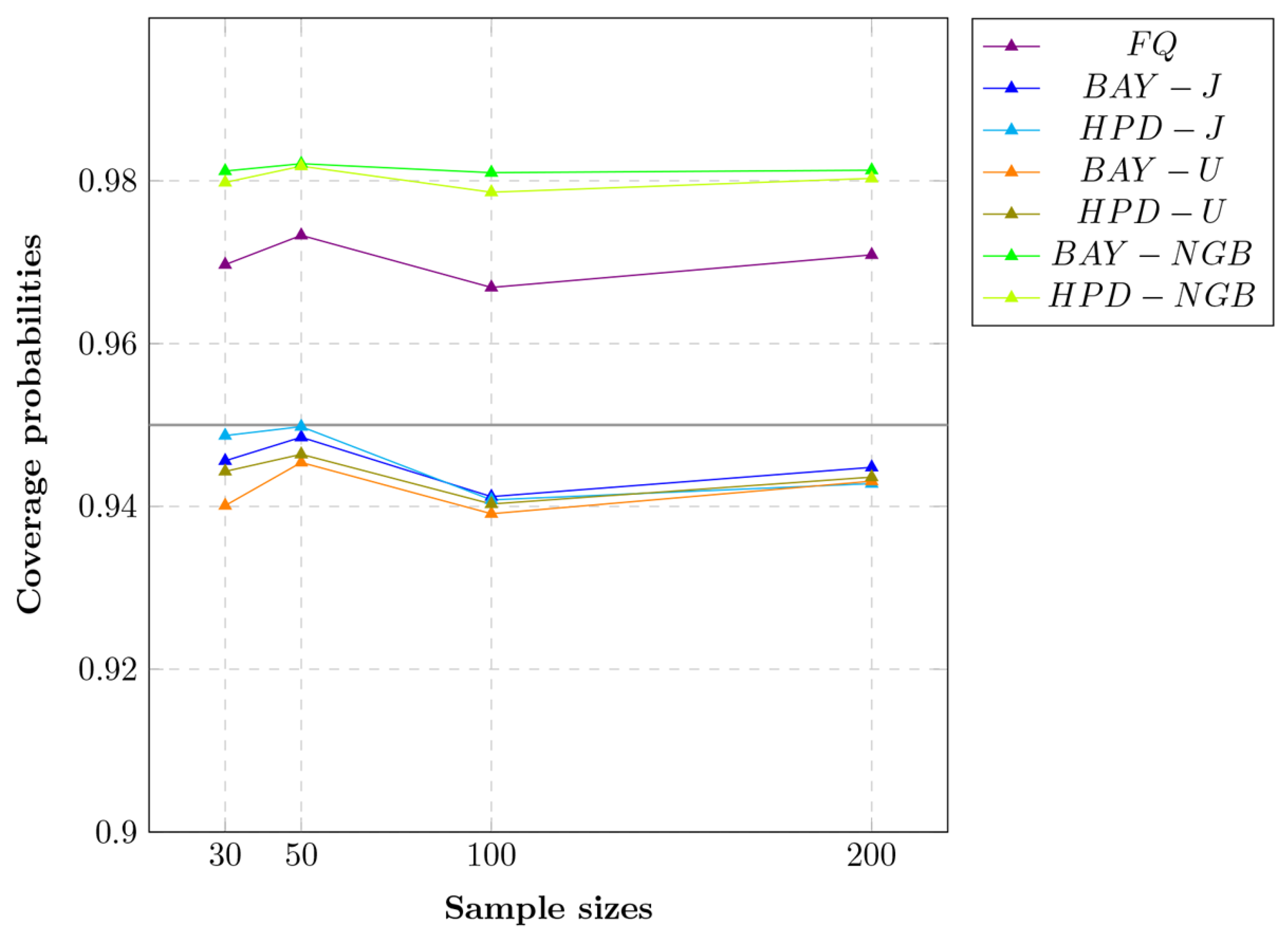
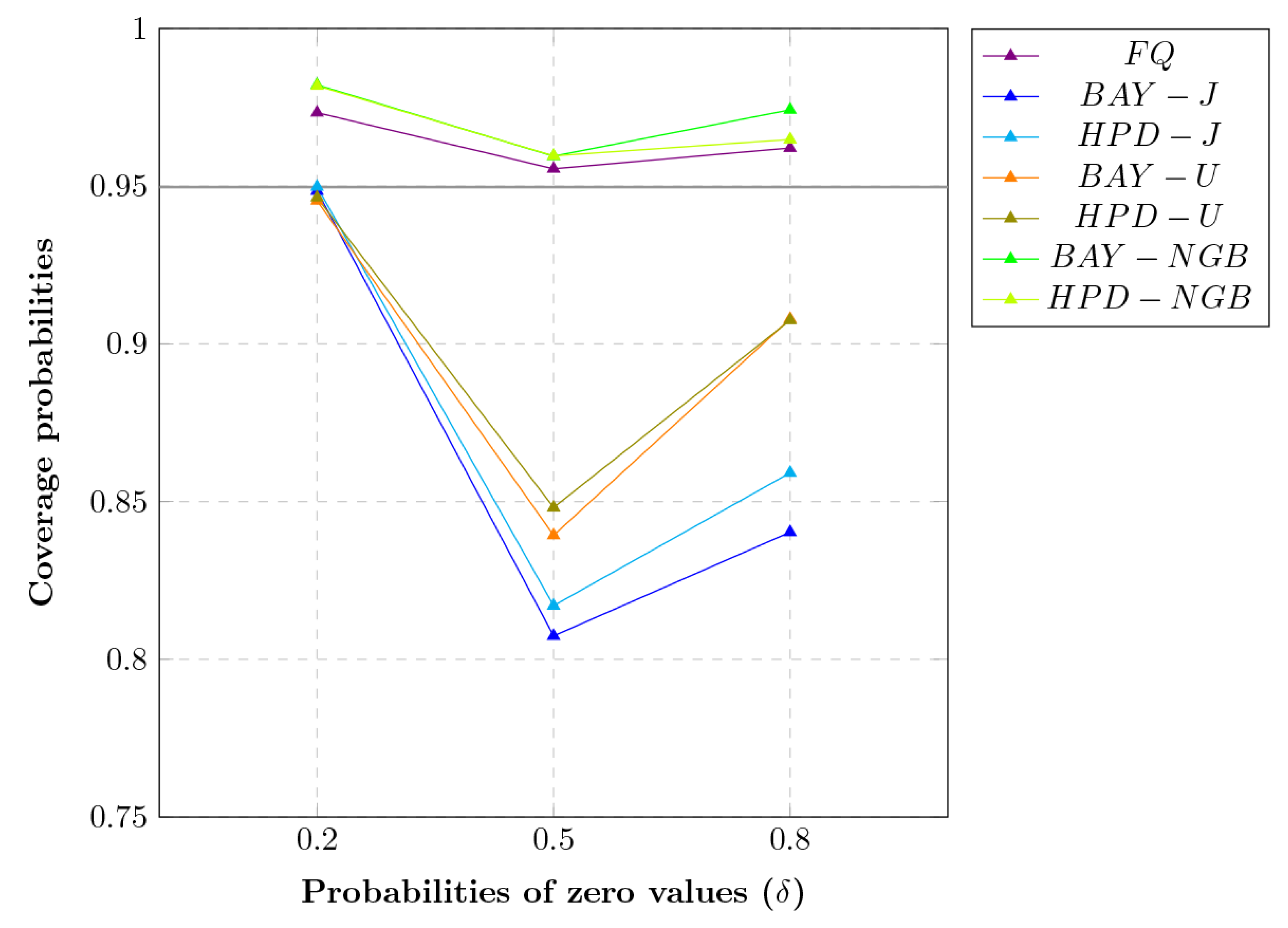
A simulation study to generate the confidence interval for the ratio of the variance of two independent delta-gamma distributions by using the proposed methods was conducted with 10,000 replications (M), 5000 repetitions (m) for FQ, and the nominal confidence level set as 0.95 using R statistical software version 4.1.0. For equal sample sizes , we used (30,30), (50,50), (100,100), or (200,200), and for unequal sample sizes , we used (30,50), (50,100), or (100,200). For the two probabilities of data containing zeros , we set shape parameters as (7.00,7.00), (7.00,7.50), (7.50,7.00), or (7.50,7.50); for , we set as (2.00,2.00), (2.00,2.50), (2.50,2.00), or (2.50,2.50); and for , we set as (1.25,1.25), (1.25,1.50), (1.50,1.25), or (1.50,1.50); we set rate parameters as (1,1) for all cases. The performances of FQ, BAY-J, HPD-J, BAY-U, HPD-U, BAY-NGB, and HPD-NGB were assessed by comparing their CPs and ALs, with the best-performing one for a particular scenario having a CP close to or greater than 0.95 and the shortest AL.
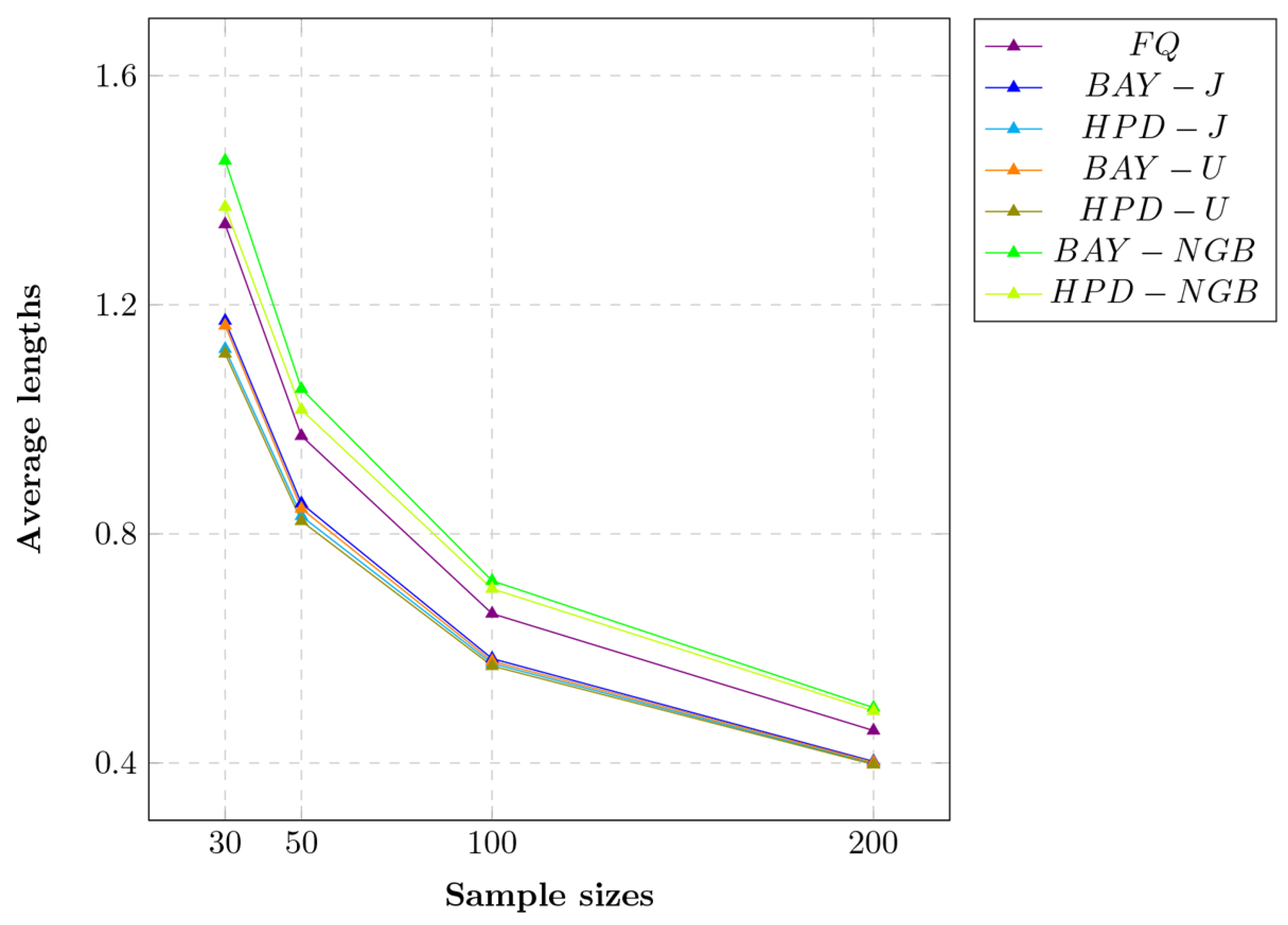
The efficacies of the various methods for the nominal two-sided confidence interval for the ratio of the variances of delta-gamma distributions with equal and unequal sample sizes in terms of their CPs and ALs are reported in Table 1 and Table 2 and Figure 1, Figure 2, Figure 3 and Figure 4: Table 1 and Table 2 report the simulation results, while Figure 1, Figure 2, Figure 3 and Figure 4 summarize the CPs and ALs from Table 1 and Table 2.
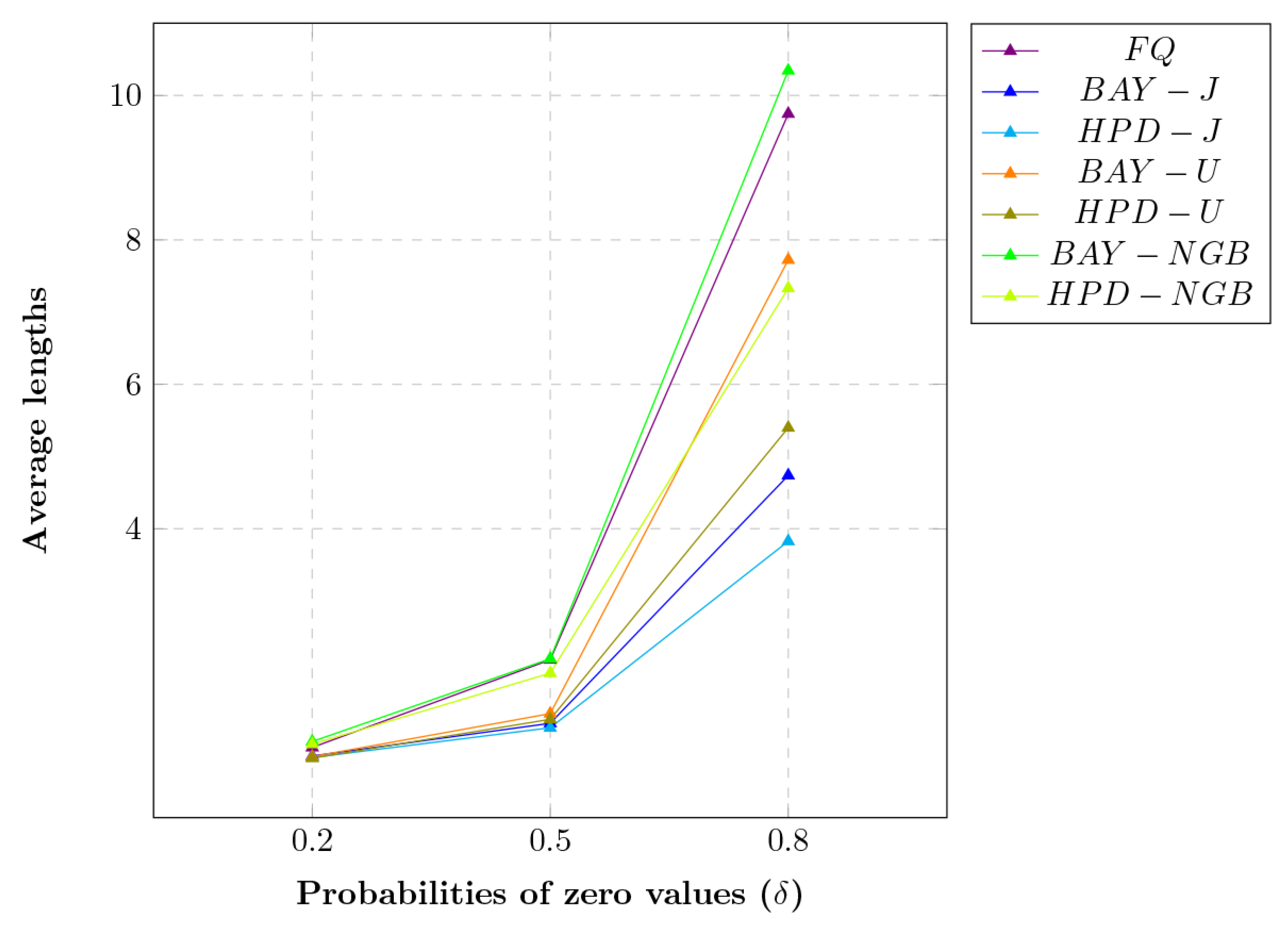
The findings show that FQ, HPD-J, HPD-U, BAY-NGB, and HPD-NGB attained CPs greater than or close to the nominal confidence level of 0.95. For small-to-moderate sample sizes, FQ, BAY-NGB, and HPD-NGB performed well for both small and large whereas the HPD-J and HPD-U performed well for small . For large , the ALs of HPD-NGB were the shortest. For large sample sizes, FQ and HPD-J performed well for small whereas HPD-U, BAY-NGB, and HPD-NGB performed well for large . For small , the ALs of FQ and HPD-J were shorter than the other methods whereas for large , the ALs of HPD-NGB were the shortest. The results in Figure 1 and Figure 3 reveal that FQ, BAY-NGB, and HPD-NGB performed well in almost all cases. Figure 2 and Figure 4 show that BAY-J and HPD-J provide the shortest ALs.
Maneerat et al. [12] proposed the confidence interval for the ratio of the variances of two delta-lognormal distributions using an HPD based on the normal-gamma prior (HPD-NG), as well as the method of variance estimates recovery (MOVER). These proposed methods were compared with existing HPD-J, HPD based on the Jeffreys’ rule prior, the generalized confidence interval (GCI), and the fiducial GCI. They found that HPD-NG performed very well in various situations while MOVER could be recommended for scenarios with small equal sample sizes. From the simulation results of the present study, it can be seen that HPD-NGB performed well for moderate-to-large sample sizes, while HPD-J and HPD-NGB both performed well for small-to-large sample sizes. Hence, both methods can be recommended for constructing the confidence interval for the ratio of the variances of two delta-gamma distributions.
4. Application of the Methods with Real Data
The performances of confidence interval methods were compared by analyzing rainfall data reported by the Upper Northern Region Irrigation Hydrology Center, Phrae province, Thailand.
4.1. Application of the Ratio of Variances of Two Delta-Gamma Distributions with Equal Sample Sizes
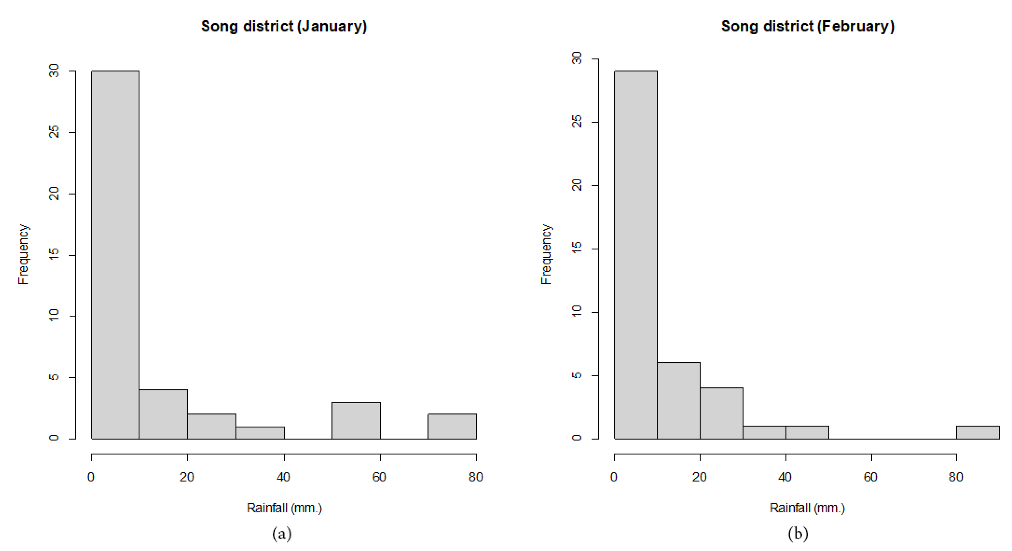
For , we used monthly rainfall data from January and February 1980 to 2021 in Song district, Phrae province, Thailand. The densities of the rainfall data are shown in Figure 5.
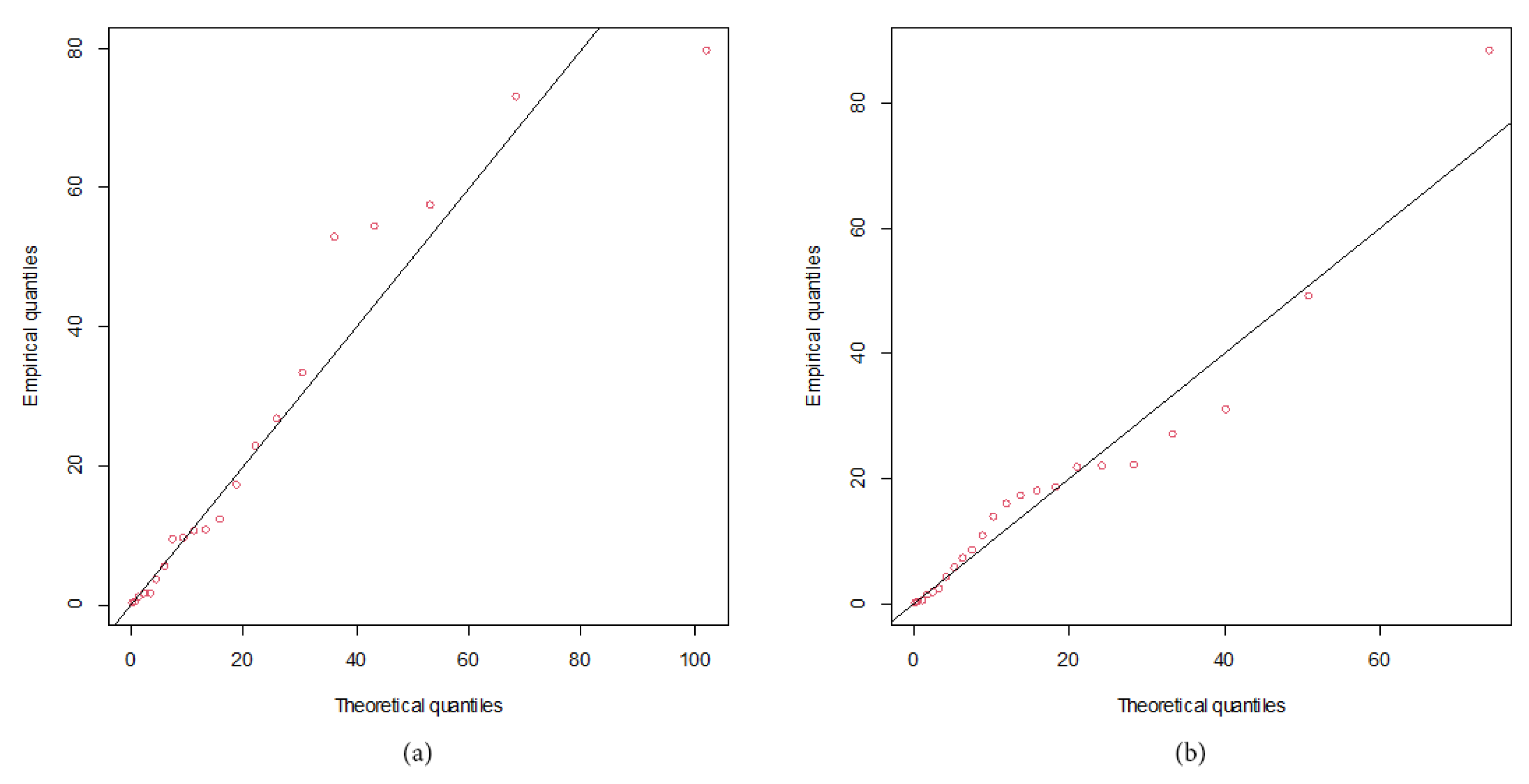
First, we attempted to fit the positive rainfall data using four models normal, lognormal, Cauchy, and gamma by using the Akaike information criterion (AIC), the results of which are reported in Table 3; the lowest AIC value was obtained by fitting with the gamma distribution, which is thus the most suitable distribution. Q-Q plots of positive rainfall data are shown in Figure 6.
The summary statistics for the rainfall in the February dataset from the Song station, , while the maximum likelihood estimators for , and are , and , respectively. Similarly, the summary statistics for the rainfall in the January dataset from the Song station are , while the maximum likelihood estimators for , and are , and are respectively. The two-sided confidence intervals results for reported in Table 4 indicate that the AL provided by HPD-U was the shortest, and thus it is the best approach for constructing the confidence interval for the ratio of the variances of two rainfall datasets with equal sample sizes from the Rong Kwang district, Phrae province, Thailand.
4.2. Application of Variances of Two Delta-Gamma Distributions with Unequal Sample Sizes
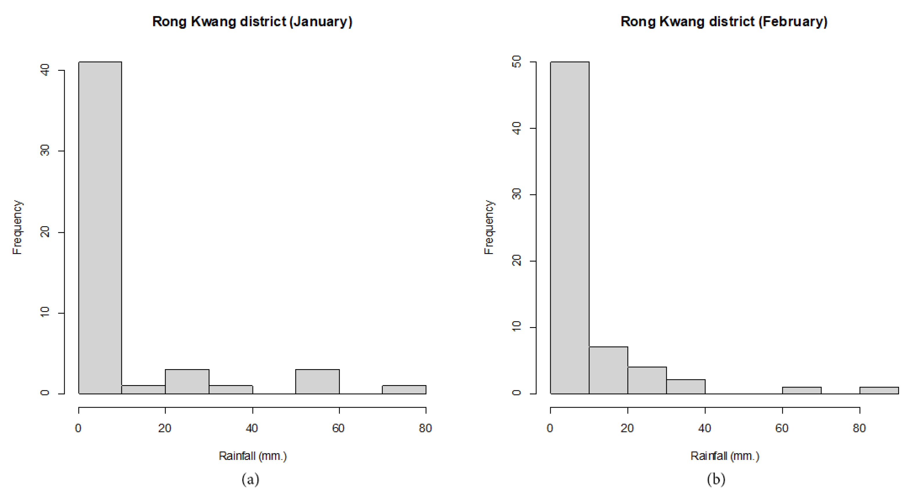
For , we used monthly rainfall data in January from 1969 to 2021 and February 1953 to 2021 in Rong Kwang district, Phrae province, Thailand. The densities of the rainfall data are shown in Figure 7.
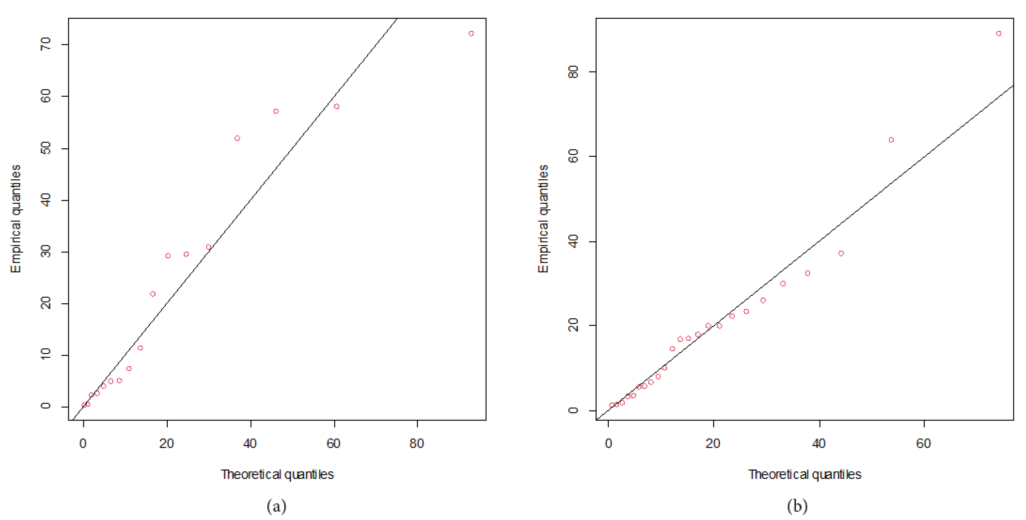
Fitting of the positive rainfall data was attempted with four models: normal, lognormal, Cauchy, and gamma, the AIC values for which are reported in Table 3. The results show that the gamma distribution is the best fit. Q-Q plots of positive rainfall data are shown in Figure 8.
The summary statistics for the rainfall in the February dataset from the Rong Kwang station, , while the maximum likelihood estimators for , and are , and , respectively. Similarly, the summary statistics for the rainfall in the January dataset from the Rong Kwang station as , while the maximum likelihood estimators for , and are , and are respectively. The two-sided confidence intervals results for reported in Table 5 indicate that the AL provided by HPD-J was the shortest, and thus it is the best approach for constructing the confidence interval for the ratio of variances of two rainfall datasets with unequal sample sizes from the Rong Kwang district, Phrae province, Thailand.
5. Conclusions
We constructed the confidence interval for the ratio of the variances of two delta-gamma distributions by using the FQ, BAY-J, HPD-J, BAY-U, HPD-U, BAY-NGB, and HPD-NGB approaches. The CPs and ALs as performance measures for the methods were assessed via Monte Carlo simulation. Our findings show that for small and large , HPD-J and HPD-NGB can be recommended for constructing the confidence interval for this scenario. Maybe other priors are more effective. Therefore, choosing priors is very important in the Bayesian method.
Author Contributions
W.K.: performed the experiments, analyzed the data, authored or reviewed drafts of the paper; S.-A.N.: concived and designed the experiments, approved the final draft; S.N.: contributed analysis tools, prepared tables. All authors have read and agreed to the published version of the manuscript.
Funding
This research received financial support from the National Science, Research, and Innovation Fund (NSRF), and King Mongkut’s University of Technology North Bangkok (Grant No. KMUTNB-FF-66-44).
Data Availability Statement
The data of monthly rainfall were obtained from the Upper Northern Region Irrigation Hydrology Center.
Acknowledgments
The authors would like to thank the referees for their valuable comments which led to the improvement. The first author wishes to express gratitude for financial support provided by the Thailand Science Achievement Scholarship (SAST).
Conflicts of Interest
The authors have declared no conflict of interest.
References
- Harvey, J.; van der Merwe, A. Bayesian confidence intervals for means and variances of lognormal and bivariate lognormal distributions. J. Stat. Plan. Inference 2012, 142, 1294–1309. [Google Scholar] [CrossRef]
- Niwitpong, S. Generalized confidence intervals for function of variances of lognormal distributions. Adv. Appl. Stat. 2017, 51, 151–163. [Google Scholar] [CrossRef]
- Puggard, W.; Niwitpong, S.A.; Niwitpong, S. Confidence intervals for the variance and difference of variances of Birnbaum-Saunders distributions. J. Stat. Comput. Simul. 2022, 92, 2829–2845. [Google Scholar] [CrossRef]
- Puggard, W.; Niwitpong, S.A.; Niwitpong, S. Confidence Intervals for Comparing the Variances of Two Independent Birnbaum—Saunders Distributions. Symmetry 2022, 14, 1492. [Google Scholar] [CrossRef]
- Krishnamoorthy, K.; Wang, X. Fiducial confidence limits and prediction limits for a gamma distribution: Censored and uncensored cases. Environmetrics 2016, 27, 479–493. [Google Scholar] [CrossRef]
- Gibbons, R.D.; Coleman, D.D. Statistical Methods for Detection and Quantification of Environmental Contamination; Wiley: Hoboken, NJ, USA, 2001. [Google Scholar]
- Aitchison, J. On the Distribution of a Positive Random Variable Having a Discrete Probability Mass at the Origin. J. Am. Stat. Assoc. 1955, 50, 901–908. [Google Scholar]
- Aitchison, J.; Brown, J.A.C. The Lognormal Distribution: With Special Reference to Its Uses in Economics London; Cambridge University Press: Cambridge, UK, 1963. [Google Scholar]
- Yosboonruang, N.; Niwitpong, S.A.; Niwitpong, S. Measuring the dispersion of rainfall using Bayesian confidence intervals for coefficient of variation of delta-lognormal distribution: A study from Thailand. PeerJ 2019, 7, e7344. [Google Scholar] [CrossRef]
- Maneerat, P.; Niwitpong, S.A.; Niwitpong, S. Bayesian confidence intervals for the difference between variances of delta-lognormal distributions. Biom. J. 2020, 62, 1769–1790. [Google Scholar] [CrossRef]
- Maneerat, P.; Niwitpong, S.A.; Niwitpong, S. Bayesian confidence intervals for variance of delta-lognormal distribution with an application to rainfall dispersion. Stat. Its Interface 2021, 14, 229–241. [Google Scholar] [CrossRef]
- Maneerat, P.; Niwitpong, S.A.; Niwitpong, S. A Bayesian approach to construct confidence intervals for comparing the rainfall dispersion in Thailand. PeerJ 2020, 8, e8502. [Google Scholar] [CrossRef] [Green Version]
- Zhang, Q.; Xu, J.; Zhao, J.; Liang, H.; Li, X. Simultaneous confidence intervals for ratios of means of zero-inflated log-normal populations. J. Stat. Comput. Simul. 2022, 92, 1113–1132. [Google Scholar] [CrossRef]
- Ren, P.; Liu, G.; Pu, X. Simultaneous confidence intervals for mean differences of multiple zero-inflated gamma distributions with applications to precipitation. Commun. Stat. Simul. Comput. 2021, 1–12. [Google Scholar] [CrossRef]
- Muralidharan, K.; Kale, B.K. Modified gamma distributions with singularity at zero. Commun. Stat. Simul. Comput. 2002, 31, 143–158. [Google Scholar] [CrossRef]
- Lecomte, J.B.; Benoît, H.P.; Ancelet, S.; Etienne, M.P.; Bel, L.; Parent, E. Compound Poisson-gamma vs. delta-gamma to handle zero-inflated continuous data under a variable sampling volume. Methods Ecol. Evol. 2013, 4, 1159–1166. [Google Scholar] [CrossRef]
- Kaewprasert, T.; Niwitpong, S.A.; Niwitpong, S. Bayesian estimation for the mean 181 of delta-gamma distributions with application to rainfall data in Thailand. PeerJ 2022, 10, e13465. [Google Scholar] [CrossRef]
- Khooriphan, W.; Niwitpong, S.A.; Niwitpong, S. Bayesian estimation of rainfall dispersion in Thailand using gamma distribution with excess zeros. PeerJ 2022, 10, e14023. [Google Scholar] [CrossRef]
- Wang, X.; Li, M.; Sun, W.; Gao, Z.; Li, X. Confidence intervals for zero-inflated gamma distribution. Commun. Stat. Simul. Comput. 2022, 1–18. [Google Scholar] [CrossRef]
- Sangnawakij, P.; Niwitpong, S.A. Confidence intervals for functions of coefficients of variation with bounded parameter spaces in two gamma distributions. Songklanakarin J. Sci. Technol. 2017, 39, 27–39. [Google Scholar]
- Krishnamoorthy, K.; Mathew, T.; Mukherjee, S. Normal-Based Methods for a Gamma Distribution. Technometrics 2008, 50, 69–78. [Google Scholar] [CrossRef]
- Li, X.; Zhou, X.; Tian, L. Interval estimation for the mean of lognormal data with excess zeros. Stat. Probab. Lett. 2013, 83, 2447–2453. [Google Scholar] [CrossRef]
- Gelman, A.; Carlin, J.B.; Stern, H.S.; Dunson, D.B.; Vehtari, A.; Rubin, D.B. Bayesian Data Analysis (Chapman & Hall/CRC Texts in Statistical Science), 3rd ed.; Chapman and Hall/CRC: Boca Raton, FL, USA, 2013. [Google Scholar]
- Casella, G.; Berger, R.L. Statistical Inference, 2nd ed.; Cengage Learning: Boston, MA, USA, 2001. [Google Scholar]
- Bolstad, W.M.; Curran, J.M. Introduction to Bayesian Statistics, 3rd ed.; Wiley: Hoboken, NJ, USA, 2016. [Google Scholar]
- Box, G.E.P.; Tiao, G.C. Bayesian Inference in Statistical Analysis; Wiley Classics: New York, NY, USA, 1973. [Google Scholar]
- Jeffreys, H. Theory of Probability; Oxford University Press: Oxford, UK, 1961. [Google Scholar]
- O’Reilly, J.X.; Mars, R.B. Bayesian Models in Cognitive Neuroscience: A Tutorial. Introd. Model-Based Cogn. Neurosci. 2015, 179–197. [Google Scholar]
- Stone, J.V. Bayes’ Rule: A Tutorial Introduction to Bayesian Analysis; Sebtel Press: Sheffield, UK, 2013. [Google Scholar]
- Kalkur, T.A.; Rao, A. Bayes estimator for coefficient of variation and inverse coefficient of variation for the normal distribution. Int. J. Stat. Syst. 2017, 12, 721–732. [Google Scholar]
- Maneerat, P.; Niwitpong, S.A. Estimating the average daily rainfall in Thailand using confidence intervals for the common mean of several delta-lognormal distributions. PeerJ 2021, 9, e10758. [Google Scholar] [CrossRef] [PubMed]
Figure 1.
Line graphs of the CPs of the methods in the simulated scenario with different sample sizes.
Figure 1.
Line graphs of the CPs of the methods in the simulated scenario with different sample sizes.

Figure 2.
Line graphs of the ALs of the methods in the simulated scenario with different sample sizes.
Figure 2.
Line graphs of the ALs of the methods in the simulated scenario with different sample sizes.

Figure 3.
Line graphs of the CPs of the methods in the simulated scenario with different probabilities of zero values.
Figure 3.
Line graphs of the CPs of the methods in the simulated scenario with different probabilities of zero values.

Figure 4.
Line graphs of the ALs of the methods in the simulated scenario with different probabilities of zero values.
Figure 4.
Line graphs of the ALs of the methods in the simulated scenario with different probabilities of zero values.

Figure 5.
The densities of the rainfall data from Song district station, Phrae province, Thailand, for (a) January and (b) February from 1980–2021.
Figure 5.
The densities of the rainfall data from Song district station, Phrae province, Thailand, for (a) January and (b) February from 1980–2021.

Figure 6.
Q-Q plots for distribution fitting of the positive rainfall data from the Song district station, Phrae province, Thailand, for (a) January and (b) February from 1980–2021.
Figure 6.
Q-Q plots for distribution fitting of the positive rainfall data from the Song district station, Phrae province, Thailand, for (a) January and (b) February from 1980–2021.

Figure 7.
The densities of the rainfall data from Rong Kwang district station, Phrae province, Thailand, for (a) January from 1969–2021 and (b) February from 1953–2021.
Figure 7.
The densities of the rainfall data from Rong Kwang district station, Phrae province, Thailand, for (a) January from 1969–2021 and (b) February from 1953–2021.

Figure 8.
Q-Q plots for distribution fitting of the positive rainfall data from the Rong Kwang district station, Phrae province, Thailand, for (a) January from 1969–2021 and (b) February from 1953–2021.
Figure 8.
Q-Q plots for distribution fitting of the positive rainfall data from the Rong Kwang district station, Phrae province, Thailand, for (a) January from 1969–2021 and (b) February from 1953–2021.


Table 1.
The CPs and (ALs) of nominal two-sided confidence interval for the ratio of variances of delta-gamma distributions .
Table 1.
The CPs and (ALs) of nominal two-sided confidence interval for the ratio of variances of delta-gamma distributions .
| CP | |||||||||
|---|---|---|---|---|---|---|---|---|---|
| (AL) | |||||||||
| FQ | BAY-J | HPD-J | BAY-U | HPD-U | BAY-NGB | HPD-NGB | |||
| 30, 30 | 0.2, 0.2 | 7.00, 7.00 | 0.9697 | 0.9456 | 0.9487 | 0.9401 | 0.9443 | 0.9812 | 0.9798 |
| (1.3406) | (1.1720) | (1.1228) | (1.1637) | (1.1147) | (1.4517) | (1.3708) | |||
| 7.00, 7.50 | 0.9684 | 0.9449 | 0.9500 | 0.9399 | 0.9471 | 0.9800 | 0.9773 | ||
| (1.1818) | (1.0453) | (0.9999) | (1.0355) | (0.9907) | (1.2858) | (1.2139) | |||
| 7.50, 7.00 | 0.9690 | 0.9447 | 0.9488 | 0.9393 | 0.9447 | 0.9805 | 0.9795 | ||
| (1.4761) | (1.3029) | (1.2500) | (1.2892) | (1.2372) | (1.6069) | (1.5201) | |||
| 7.50, 7.50 | 0.9758 | 0.9542 | 0.9568 | 0.9506 | 0.9520 | 0.9846 | 0.9830 | ||
| (1.3018) | (1.1622) | (1.1136) | (1.1470) | (1.0995) | (1.4230) | (1.3457) | |||
| 0.5, 0.5 | 2.00, 2.00 | 0.9543 | 0.8024 | 0.8214 | 0.8558 | 0.8755 | 0.9609 | 0.9590 | |
| (3.5398) | (1.9996) | (1.8291) | (2.4537) | (2.1768) | (3.5356) | (3.0144) | |||
| 2.00, 2.50 | 0.9579 | 0.8046 | 0.8101 | 0.8570 | 0.8679 | 0.9633 | 0.9540 | ||
| (2.2508) | (1.2767) | (1.1654) | (1.5877) | (1.4052) | (2.2075) | (1.9006) | |||
| 2.50, 2.00 | 0.9528 | 0.8064 | 0.8274 | 0.8589 | 0.8746 | 0.9593 | 0.9637 | ||
| (4.6023) | (2.6154) | (2.4322) | (3.1508) | (2.8538) | (4.6543) | (4.0229) | |||
| 2.50, 2.50 | 0.9531 | 0.8046 | 0.8194 | 0.8619 | 0.8647 | 0.9594 | 0.9607 | ||
| (2.9341) | (1.6747) | (1.5549) | (2.0430) | (1.8489) | (2.9196) | (2.5507) | |||
| 0.8, 0.8 | 1.25, 1.25 | 0.9604 | 0.8441 | 0.8689 | 0.9474 | 0.9456 | 0.9749 | 0.9692 | |
| (54.7822) | (15.1368) | (9.0762) | (187.644) | (47.1799) | (60.6257) | (27.3089) | |||
| 1.25, 1.50 | 0.9662 | 0.8464 | 0.8663 | 0.9510 | 0.9470 | 0.9786 | 0.9686 | ||
| (33.1790) | (9.4095) | (5.7188) | (111.917) | (29.4096) | (33.5318) | (15.7383) | |||
| 1.50, 1.25 | 0.9636 | 0.8481 | 0.8797 | 0.9495 | 0.9468 | 0.9771 | 0.9727 | ||
| (57.4290) | (16.7939) | (10.7268) | (166.582) | (45.5388) | (62.8024) | (30.5099) | |||
| 1.50, 1.50 | 0.9676 | 0.8568 | 0.8731 | 0.9554 | 0.9491 | 0.9803 | 0.9743 | ||
| (34.5386) | (10.4576) | (6.7205) | (102.669) | (28.7895) | (36.1227) | (17.8842) | |||
| 50, 50 | 0.2, 0.2 | 7.00, 7.00 | 0.9733 | 0.9485 | 0.9498 | 0.9454 | 0.9464 | 0.9821 | 0.9818 |
| (0.9710) | (0.8531) | (0.8311) | (0.8440) | (0.8224) | (1.0532) | (1.0167) | |||
| 7.00, 7.50 | 0.9694 | 0.9482 | 0.9471 | 0.9448 | 0.9430 | 0.9822 | 0.9795 | ||
| (0.8638) | (0.7674) | (0.7468) | (0.7583) | (0.7382) | (0.9417) | (0.9087) | |||
| 7.50, 7.00 | 0.9708 | 0.9516 | 0.9505 | 0.9481 | 0.9474 | 0.9814 | 0.9835 | ||
| (1.0778) | (0.9573) | (0.9334) | (0.9453) | (0.9221) | (1.1762) | (1.1364) | |||
| 7.50, 7.50 | 0.9723 | 0.9540 | 0.9543 | 0.9499 | 0.9499 | 0.9852 | 0.9810 | ||
| (0.9496) | (0.8521) | (0.8301) | (0.8401) | (0.8188) | (1.0408) | (1.0053) | |||
| (AL) | |||||||||
| FQ | BAY-J | HPD-J | BAY-U | HPD-U | BAY-NGB | HPD-NGB | |||
| 0.5, 0.5 | 2.00, 2.00 | 0.9555 | 0.8074 | 0.8170 | 0.8393 | 0.8481 | 0.9595 | 0.9596 | |
| (2.1853) | (1.3055) | (1.2436) | (1.4396) | (1.3608) | (2.1998) | (1.9997) | |||
| 2.00, 2.50 | 0.9524 | 0.8000 | 0.8074 | 0.8360 | 0.8367 | 0.9579 | 0.9489 | ||
| (1.4219) | (0.8503) | (0.8090) | (0.9437) | (0.8905) | (1.4160) | (1.2965) | |||
| 2.50, 2.00 | 0.9533 | 0.7989 | 0.8138 | 0.8307 | 0.8463 | 0.9592 | 0.9625 | ||
| (2.9496) | (1.7637) | (1.6953) | (1.9309) | (1.8438) | (2.9917) | (2.7412) | |||
| 2.50, 2.50 | 0.9566 | 0.7966 | 0.8056 | 0.8297 | 0.8389 | 0.9596 | 0.9593 | ||
| (1.8968) | (1.1338) | (1.0888) | (1.2506) | (1.1928) | (1.9017) | (1.7557) | |||
| 0.8, 0.8 | 1.25, 1.25 | 0.9621 | 0.8403 | 0.8591 | 0.9079 | 0.9075 | 0.9742 | 0.9648 | |
| (9.7449) | (4.7376) | (3.8265) | (7.7233) | (5.3985) | (10.3437) | (7.3304) | |||
| 1.25, 1.50 | 0.9583 | 0.8422 | 0.8540 | 0.9045 | 0.9088 | 0.9712 | 0.9634 | ||
| (6.7461) | (3.3189) | (2.6700) | (5.6071) | (3.8850) | (6.9155) | (4.9549) | |||
| 1.50, 1.25 | 0.9605 | 0.8470 | 0.8746 | 0.9055 | 0.9201 | 0.9727 | 0.9703 | ||
| (12.0438) | (6.0132) | (4.9732) | (9.2776) | (6.7417) | (13.0570) | (9.4220) | |||
| 1.50, 1.50 | 0.9621 | 0.8454 | 0.8643 | 0.9086 | 0.9138 | 0.9736 | 0.9681 | ||
| (8.1384) | (4.1292) | (3.4129) | (6.4968) | (4.7229) | (8.5396) | (6.2547) | |||
| 100, 100 | 0.2, 0.2 | 7.00, 7.00 | 0.9669 | 0.9412 | 0.9408 | 0.9391 | 0.9403 | 0.9810 | 0.9786 |
| (0.6607) | (0.5822) | (0.5738) | (0.5777) | (0.5694) | (0.7181) | (0.7042) | |||
| 7.00, 7.50 | 0.9720 | 0.9456 | 0.9468 | 0.9433 | 0.9452 | 0.9841 | 0.9826 | ||
| (0.5827) | (0.5186) | (0.5109) | (0.5145) | (0.5068) | (0.6364) | (0.6240) | |||
| 7.50, 7.00 | 0.9731 | 0.9519 | 0.9528 | 0.9499 | 0.9502 | 0.9828 | 0.9808 | ||
| (0.7294) | (0.6491) | (0.6399) | (0.6433) | (0.6344) | (0.7966) | (0.7816) | |||
| 7.50, 7.50 | 0.9742 | 0.9555 | 0.9534 | 0.9534 | 0.9518 | 0.9846 | 0.9835 | ||
| (0.6452) | (0.5804) | (0.5718) | (0.5751) | (0.5669) | (0.7083) | (0.6949) | |||
| 0.5, 0.5 | 2.00, 2.00 | 0.9537 | 0.8008 | 0.8045 | 0.8160 | 0.8188 | 0.9581 | 0.9538 | |
| (1.3306) | (0.8227) | (0.8030) | (0.8586) | (0.8366) | (1.3450) | (1.2799) | |||
| 2.00, 2.50 | 0.9496 | 0.7950 | 0.7932 | 0.8103 | 0.8101 | 0.9539 | 0.9465 | ||
| (0.8744) | (0.5394) | (0.5260) | (0.5645) | (0.5497) | (0.8795) | (0.8403) | |||
| 2.50, 2.00 | 0.9497 | 0.7949 | 0.8051 | 0.8095 | 0.8213 | 0.9533 | 0.9600 | ||
| (1.8266) | (1.1256) | (1.1039) | (1.1716) | (1.1474) | (1.8542) | (1.7716) | |||
| 2.50, 2.50 | 0.9532 | 0.7870 | 0.7912 | 0.8026 | 0.8081 | 0.9565 | 0.9532 | ||
| (1.1874) | (0.7289) | (0.7142) | (0.7614) | (0.7449) | (1.1976) | (1.1488) | |||
| 0.8, 0.8 | 1.25, 1.25 | 0.9553 | 0.8310 | 0.8440 | 0.8621 | 0.8755 | 0.9668 | 0.9637 | |
| (3.7848) | (2.2414) | (2.0428) | (2.5366) | (2.2693) | (4.0075) | (3.3653) | |||
| 1.25, 1.50 | 0.9592 | 0.8386 | 0.8420 | 0.8708 | 0.8723 | 0.9702 | 0.9588 | ||
| (2.5811) | (1.5459) | (1.4084) | (1.7612) | (1.5750) | (2.6887) | (2.2802) | |||
| 1.50, 1.25 | 0.9565 | 0.8366 | 0.8580 | 0.8687 | 0.8841 | 0.9673 | 0.9727 | ||
| (4.8404) | (2.9052) | (2.6763) | (3.2390) | (2.9372) | (5.1819) | (4.3894) | |||
| 1.50, 1.50 | 0.9639 | 0.8433 | 0.8571 | 0.8750 | 0.8848 | 0.9740 | 0.9690 | ||
| (3.2934) | (2.0003) | (1.8424) | (2.2460) | (2.0369) | (3.4707) | (2.9718) | |||
| 200, 200 | 0.2, 0.2 | 7.00, 7.00 | 0.9709 | 0.9448 | 0.9428 | 0.9431 | 0.9436 | 0.9813 | 0.9803 |
| (0.4566) | (0.4027) | (0.3990) | (0.4010) | (0.3973) | (0.4966) | (0.4908) | |||
| 7.00, 7.50 | 0.9721 | 0.9511 | 0.9486 | 0.9479 | 0.9470 | 0.9841 | 0.9828 | ||
| (0.4044) | (0.3601) | (0.3567) | (0.3584) | (0.3551) | (0.4419) | (0.4367) | |||
| 7.50, 7.00 | 0.9711 | 0.9510 | 0.9505 | 0.9486 | 0.9492 | 0.9819 | 0.9821 | ||
| (0.5060) | (0.4506) | (0.4465) | (0.4484) | (0.4444) | (0.5529) | (0.5465) | |||
| 7.50, 7.50 | 0.9744 | 0.9529 | 0.9523 | 0.9506 | 0.9521 | 0.9853 | 0.9847 | ||
| (0.4477) | (0.4030) | (0.3992) | (0.4009) | (0.3972) | (0.4919) | (0.4862) | |||
| (AL) | |||||||||
| FQ | BAY-J | HPD-J | BAY-U | HPD-U | BAY-NGB | HPD-NGB | |||
| 0.5, 0.5 | 2.00, 2.00 | 0.9531 | 0.7896 | 0.7923 | 0.7974 | 0.7988 | 0.9562 | 0.9532 | |
| (0.8838) | (0.5547) | (0.5473) | (0.5659) | (0.5581) | (0.8953) | (0.8716) | |||
| 2.00, 2.50 | 0.9502 | 0.7895 | 0.7845 | 0.7979 | 0.7916 | 0.9533 | 0.9470 | ||
| (0.5793) | (0.3621) | (0.3570) | (0.3700) | (0.3646) | (0.5851) | (0.5708) | |||
| 2.50, 2.00 | 0.9478 | 0.7830 | 0.7887 | 0.7900 | 0.7968 | 0.9506 | 0.9566 | ||
| (1.2195) | (0.7615) | (0.7529) | (0.7765) | (0.7675) | (1.2360) | (1.2058) | |||
| 2.50, 2.50 | 0.9536 | 0.7918 | 0.7927 | 0.8012 | 0.8012 | 0.9575 | 0.9574 | ||
| (0.7949) | (0.4934) | (0.4876) | (0.5037) | (0.4976) | (0.8034) | (0.7852) | |||
| 0.8, 0.8 | 1.25, 1.25 | 0.9534 | 0.8263 | 0.8346 | 0.8425 | 0.8487 | 0.9645 | 0.9607 | |
| (2.0672) | (1.3182) | (1.2591) | (1.3814) | (1.3145) | (2.1786) | (1.9832) | |||
| 1.25, 1.50 | 0.9556 | 0.8360 | 0.8333 | 0.8490 | 0.8501 | 0.9668 | 0.9573 | ||
| (1.4357) | (0.9237) | (0.8822) | (0.9709) | (0.9235) | (1.5058) | (1.3793) | |||
| 1.50, 1.25 | 0.9579 | 0.8316 | 0.8474 | 0.8470 | 0.8614 | 0.9667 | 0.9718 | ||
| (2.6965) | (1.7363) | (1.6663) | (1.8096) | (1.7314) | (2.8603) | (2.6168) | |||
| 1.50,1.50 | 0.9605 | 0.8403 | 0.8446 | 0.8532 | 0.8592 | 0.9707 | 0.9642 | ||
| (1.8546) | (1.2043) | (1.1559) | (1.2597) | (1.2054) | (1.9569) | (1.8021) | |||
Table 2.
The CPs and (ALs) of nominal two-sided confidence interval for the ratio of variances of delta-gamma distributions .
Table 2.
The CPs and (ALs) of nominal two-sided confidence interval for the ratio of variances of delta-gamma distributions .
| CP | |||||||||
|---|---|---|---|---|---|---|---|---|---|
| (AL) | |||||||||
| FQ | BAY-J | HPD-J | BAY-U | HPD-U | BAY-NGB | HPD-NGB | |||
| 30, 50 | 0.2, 0.2 | 7.00, 7.00 | 0.9697 | 0.9432 | 0.9445 | 0.9387 | 0.9475 | 0.9808 | 0.9786 |
| (1.1937) | (1.0045) | (0.9722) | (1.0338) | (0.9966) | (1.2593) | (1.2036) | |||
| 7.00, 7.50 | 0.9738 | 0.9491 | 0.9469 | 0.9461 | 0.9501 | 0.9844 | 0.9804 | ||
| (1.0568) | (0.8970) | (0.8678) | (0.9217) | (0.8883) | (1.1195) | (1.0700) | |||
| 7.50, 7.00 | 0.9727 | 0.9512 | 0.9511 | 0.9468 | 0.9532 | 0.9816 | 0.9838 | ||
| (1.3123) | (1.1185) | (1.0848) | (1.1449) | (1.1065) | (1.3939) | (1.3349) | |||
| 7.50, 7.50 | 0.9711 | 0.9515 | 0.9495 | 0.9463 | 0.9533 | 0.9819 | 0.9822 | ||
| (1.1640) | (1.0001) | (0.9692) | (1.0229) | (0.9878) | (1.2405) | (1.1878) | |||
| 0.5, 0.5 | 2.00, 2.00 | 0.9537 | 0.7999 | 0.8181 | 0.8427 | 0.8689 | 0.9586 | 0.9581 | |
| (3.0302) | (1.7232) | (1.5584) | (2.1715) | (1.8961) | (2.8930) | (2.5193) | |||
| 2.00, 2.50 | 0.9520 | 0.8020 | 0.8088 | 0.8451 | 0.8628 | 0.9558 | 0.9516 | ||
| (2.0151) | (1.1480) | (1.0336) | (1.4625) | (1.2705) | (1.9013) | (1.6621) | |||
| 2.50, 2.00 | 0.9544 | 0.8059 | 0.8238 | 0.8446 | 0.8726 | 0.9571 | 0.9659 | ||
| (3.9549) | (2.2632) | (2.0781) | (2.7946) | (2.4900) | (3.8104) | (3.3632) | |||
| 2.50, 2.50 | 0.9521 | 0.7984 | 0.8141 | 0.8402 | 0.8645 | 0.9564 | 0.9578 | ||
| (2.5824) | (1.4775) | (1.3537) | (1.8419) | (1.6371) | (2.4630) | (2.1867) | |||
| 0.8, 0.8 | 1.25, 1.25 | 0.9619 | 0.8431 | 0.8749 | 0.9197 | 0.9569 | 0.9753 | 0.9718 | |
| (40.0928) | (11.3179) | (6.8256) | (156.047) | (40.3903) | (36.1470) | (16.9783) | |||
| 1.25, 1.50 | 0.9611 | 0.8384 | 0.8654 | 0.9198 | 0.9548 | 0.9745 | 0.9703 | ||
| (27.1107) | (7.7188) | (4.6975) | (107.454) | (27.9729) | (23.8861) | (11.3980) | |||
| 1.50, 1.25 | 0.9592 | 0.8421 | 0.8754 | 0.9165 | 0.9576 | 0.9731 | 0.9757 | ||
| (41.5169) | (12.6202) | (8.0997) | (144.186) | (39.7663) | (37.9083) | (19.2347) | |||
| 1.50, 1.50 | 0.9633 | 0.8504 | 0.8767 | 0.9244 | 0.9591 | 0.9765 | 0.9752 | ||
| (27.9288) | (8.5264) | (5.4643) | (98.4976) | (27.3681) | (24.8532) | (12.6009) | |||
| (AL) | |||||||||
| FQ | BAY-J | HPD-J | BAY-U | HPD-U | BAY-NGB | HPD-NGB | |||
| 50, 100 | 0.2, 0.2 | 7.00, 7.00 | 0.9723 | 0.9448 | 0.9447 | 0.9431 | 0.9465 | 0.9822 | 0.9823 |
| (0.8419) | (0.7190) | (0.7066) | (0.7296) | (0.7159) | (0.8958) | (0.8735) | |||
| 7.00, 7.50 | 0.9700 | 0.9441 | 0.9404 | 0.9434 | 0.9429 | 0.9809 | 0.9807 | ||
| (0.7452) | (0.6412) | (0.6300) | (0.6503) | (0.6379) | (0.7959) | (0.7760) | |||
| 7.50, 7.00 | 0.9750 | 0.9528 | 0.9505 | 0.9499 | 0.9531 | 0.9857 | 0.9832 | ||
| (0.9235) | (0.7996) | (0.7869) | (0.8093) | (0.7954) | (0.9911) | (0.9675) | |||
| 7.50, 7.50 | 0.9743 | 0.9532 | 0.9524 | 0.9503 | 0.9549 | 0.9843 | 0.9857 | ||
| (0.8218) | (0.7160) | (0.7042) | (0.7240) | (0.7113) | (0.8835) | (0.8623) | |||
| 0.5, 0.5 | 2.00, 2.00 | 0.9511 | 0.7965 | 0.8092 | 0.8201 | 0.8364 | 0.9548 | 0.9550 | |
| (1.8500) | (1.1130) | (1.0490) | (1.2452) | (1.1620) | (1.8027) | (1.6689) | |||
| 2.00, 2.50 | 0.9529 | 0.8045 | 0.7980 | 0.8286 | 0.8354 | 0.9597 | 0.9509 | ||
| (1.2170) | (0.7311) | (0.6876) | (0.8217) | (0.7651) | (1.1809) | (1.0969) | |||
| 2.50, 2.00 | 0.9494 | 0.7868 | 0.7985 | 0.8093 | 0.8317 | 0.9515 | 0.9589 | ||
| (2.4361) | (1.4641) | (1.3922) | (1.6248) | (1.5318) | (2.3858) | (2.2273) | |||
| 2.50, 2.50 | 0.9564 | 0.7990 | 0.8009 | 0.8259 | 0.8338 | 0.9596 | 0.9584 | ||
| (1.6124) | (0.9668) | (0.9177) | (1.0792) | (1.0155) | (1.5698) | (1.4699) | |||
| 0.8, 0.8 | 1.25, 1.25 | 0.9585 | 0.8335 | 0.8642 | 0.8827 | 0.9191 | 0.9701 | 0.9687 | |
| (7.7112) | (3.8873) | (3.1102) | (6.9755) | (4.7917) | (7.2172) | (5.3521) | |||
| 1.25, 1.50 | 0.9586 | 0.8444 | 0.8598 | 0.8885 | 0.9210 | 0.9707 | 0.9642 | ||
| (5.4096) | (2.7443) | (2.1945) | (4.9852) | (3.4183) | (5.0004) | (3.7310) | |||
| 1.50, 1.25 | 0.9583 | 0.8389 | 0.8723 | 0.8782 | 0.9251 | 0.9683 | 0.9734 | ||
| (9.2636) | (4.7883) | (3.9429) | (8.0576) | (5.7833) | (8.8128) | (6.7038) | |||
| 1.50, 1.50 | 0.9584 | 0.8428 | 0.8637 | 0.8847 | 0.9225 | 0.9708 | 0.9698 | ||
| (6.4244) | (3.3469) | (2.7510) | (5.6927) | (4.0797) | (6.0353) | (4.6216) | |||
| 100, 200 | 0.2, 0.2 | 7.00, 7.00 | 0.9726 | 0.9471 | 0.9469 | 0.9448 | 0.9474 | 0.9837 | 0.9828 |
| (0.5701) | (0.4950) | (0.4901) | (0.4972) | (0.4922) | (0.6133) | (0.6047) | |||
| 7.00, 7.50 | 0.9712 | 0.9477 | 0.9476 | 0.9453 | 0.9475 | 0.9832 | 0.9813 | ||
| (0.5074) | (0.4435) | (0.4391) | (0.4453) | (0.4408) | (0.5475) | (0.5398) | |||
| 7.50, 7.00 | 0.9741 | 0.9547 | 0.9551 | 0.9544 | 0.9544 | 0.9845 | 0.9850 | ||
| (0.6277) | (0.5523) | (0.5472) | (0.5541) | (0.5489) | (0.6803) | (0.6711) | |||
| 7.50, 7.50 | 0.9719 | 0.9535 | 0.9521 | 0.9511 | 0.9530 | 0.9849 | 0.9839 | ||
| (0.5578) | (0.4943) | (0.4897) | (0.4958) | (0.4911) | (0.6065) | (0.5983) | |||
| 0.5, 0.5 | 2.00, 2.00 | 0.9528 | 0.7967 | 0.7992 | 0.8076 | 0.8126 | 0.9565 | 0.9553 | |
| (1.1466) | (0.7116) | (0.6903) | (0.7464) | (0.7228) | (1.1408) | (1.0965) | |||
| 2.00, 2.50 | 0.9510 | 0.7922 | 0.7890 | 0.8073 | 0.8071 | 0.9553 | 0.9469 | ||
| (0.7627) | (0.4719) | (0.4571) | (0.4964) | (0.4800) | (0.7566) | (0.7288) | |||
| 2.50, 2.00 | 0.9508 | 0.7853 | 0.7953 | 0.7988 | 0.8084 | 0.9541 | 0.9584 | ||
| (1.5382) | (0.9498) | (0.9258) | (0.9938) | (0.9668) | (1.5336) | (1.4799) | |||
| 2.50, 2.50 | 0.9528 | 0.7896 | 0.7911 | 0.8018 | 0.8060 | 0.9574 | 0.9557 | ||
| (1.0160) | (0.6249) | (0.6084) | (0.6556) | (0.6371) | (1.0104) | (0.9772) | |||
| 0.8, 0.8 | 1.25, 1.25 | 0.9558 | 0.8257 | 0.8417 | 0.8491 | 0.8706 | 0.9661 | 0.9645 | |
| (3.0752) | (1.8653) | (1.6982) | (2.1607) | (1.9264) | (3.0750) | (2.6785) | |||
| 1.25, 1.50 | 0.9582 | 0.8405 | 0.8464 | 0.8625 | 0.8798 | 0.9678 | 0.9601 | ||
| (2.1497) | (1.3110) | (1.1934) | (1.5267) | (1.3603) | (2.1382) | (1.8719) | |||
| 1.50, 1.25 | 0.9587 | 0.8350 | 0.8555 | 0.8563 | 0.8855 | 0.9684 | 0.9725 | ||
| (3.8343) | (2.3578) | (2.1723) | (2.6898) | (2.4330) | (3.8684) | (3.4072) | |||
| 1.50, 1.50 | 0.9614 | 0.8415 | 0.8575 | 0.8601 | 0.8875 | 0.9711 | 0.9711 | ||
| (2.6930) | (1.6670) | (1.5355) | (1.9107) | (1.7274) | (2.7070) | (2.3962) | |||
Table 3.
AIC results of positive rainfall data.
| Rainfall Station | Normal | Lognormal | Cauchy | Gamma |
|---|---|---|---|---|
| Song (January) | 198.35 | 178.43 | 198.48 | 175.61 |
| Song (February) | 205.29 | 183.56 | 198.98 | 178.75 |
| Rong Kwang (January) | 158.92 | 145.36 | 164.03 | 143.15 |
| Rong Kwang (February) | 216.35 | 196.28 | 211.51 | 195.57 |
Table 4.
The two-sided confidence intervals for the ratio of variances of rainfall datasets from Song district, Phrae province, Thailand.
Table 4.
The two-sided confidence intervals for the ratio of variances of rainfall datasets from Song district, Phrae province, Thailand.
| Methods | Confidence Intervals for | Length of Intervals | |
|---|---|---|---|
| Lower | Upper | ||
| FQ | 0.0011 | 5.5189 | 5.5178 |
| BAY-J | 0.1374 | 0.1790 | 0.0416 |
| HPD-J | 0.1366 | 0.1776 | 0.0410 |
| BAY-U | 0.1399 | 0.1800 | 0.0401 |
| HPD-U | 0.1395 | 0.1790 | 0.0395 |
| BAY-NGB | 0.1386 | 0.1791 | 0.0405 |
| HPD-NGB | 0.1384 | 0.1788 | 0.0404 |
Table 5.
The two-sided confidence intervals for the ratio of variances of rainfall datasets from Rong Kwang district, Phrae province, Thailand.
Table 5.
The two-sided confidence intervals for the ratio of variances of rainfall datasets from Rong Kwang district, Phrae province, Thailand.
| Methods | Confidence Intervals for | Length of Intervals | |
|---|---|---|---|
| Lower | Upper | ||
| FQ | 0.0023 | 18.8012 | 18.7989 |
| BAY-J | 0.3574 | 0.5822 | 0.2248 |
| HPD-J | 0.3483 | 0.5685 | 0.2202 |
| BAY-U | 0.3534 | 0.5904 | 0.2370 |
| HPD-U | 0.3420 | 0.5715 | 0.2295 |
| BAY-NGB | 0.3597 | 0.5924 | 0.2327 |
| HPD-NGB | 0.3511 | 0.5757 | 0.2246 |
Publisher’s Note: MDPI stays neutral with regard to jurisdictional claims in published maps and institutional affiliations. |
© 2022 by the authors. Licensee MDPI, Basel, Switzerland. This article is an open access article distributed under the terms and conditions of the Creative Commons Attribution (CC BY) license (https://creativecommons.org/licenses/by/4.0/).
Share and Cite
MDPI and ACS Style
Khooriphan, W.; Niwitpong, S.-A.; Niwitpong, S. Confidence Intervals for the Ratio of Variances of Delta-Gamma Distributions with Applications. Axioms 2022, 11, 689. https://doi.org/10.3390/axioms11120689
AMA Style
Khooriphan W, Niwitpong S-A, Niwitpong S. Confidence Intervals for the Ratio of Variances of Delta-Gamma Distributions with Applications. Axioms. 2022; 11(12):689. https://doi.org/10.3390/axioms11120689
Chicago/Turabian StyleKhooriphan, Wansiri, Sa-Aat Niwitpong, and Suparat Niwitpong. 2022. "Confidence Intervals for the Ratio of Variances of Delta-Gamma Distributions with Applications" Axioms 11, no. 12: 689. https://doi.org/10.3390/axioms11120689
Note that from the first issue of 2016, this journal uses article numbers instead of page numbers. See further details here.