
Geometric Study of 2D-Wave Equations in View of K-Symbol Airy Functions


1
Department of Mathematics and Sciences, College of Humanities and Sciences, Ajman University, Ajman P.O. Box 346 00000, United Arab Emirates
2
Nonlinear Dynamics Research Center (NDRC), Ajman University, Ajman P.O. Box 346 00000, United Arab Emirates
3
Mathematics Research Center, Department of Mathematics, Near East University, Near East Boulevard, TRNC Mersin 10, Nicosia 99138, Turkey
*
Author to whom correspondence should be addressed.
†
These authors contributed equally to this work.
Axioms 2022, 11(11), 590; https://doi.org/10.3390/axioms11110590
Submission received: 3 October 2022
/
Revised: 13 October 2022
/
Accepted: 17 October 2022
/
Published: 26 October 2022
(This article belongs to the Special Issue New Developments in Geometric Function Theory)
Abstract
:The notion of k-symbol special functions has recently been introduced. This new concept offers many interesting geometric properties for these special functions including logarithmic convexity. The aim of the present paper is to exploit essentially two-dimensional wave propagation in the earth-ionosphere wave path using k-symbol Airy functions (KAFs) in the open unit disk. It is shown that the standard wave-mode working formula may be determined by orthogonality considerations without the use of intricate justifications of the complex plane. By taking into account the symmetry-convex depiction of the KAFs, the formula combination is derived.
Keywords:
analytic function; inequalities; univalent function; open unit disk; symmetric differential operator; airy functions; normalization; complex wave equation; k-symbol calculusMSC:
30C45; 30C15; 33C101. Introduction
When Diaz and Pariguan [1] were assessing Feynman integrals, they introduced and researched k-gamma functions. Because they provide a generic integral representation of the relevant functions, these integrals are fundamentally important in high-energy physics [2]. K-gamma functions have since been developed which have a variety of consequences for mathematics and applications. In light of significant applications in quantum chemistry, Karwowski and Witek [3] employed k-special functions for determining the solution of the complex Schrodinger equation for the harmonium and similar designs. In their collected papers, there is a great deal of attention to the theory of measurement and combination versions for the k-maximizing factorial numbers that are used as examples as well as to the combinatorics of the Pochhammer k-symbol.
K-gamma functions were employed for combination analysis by Lackner and Lackner [4] in light of significant applications in statistics. Applications of various k-gamma function types have eliminated the major concerns, and, as a result, multiple publications analyzing k-gamma functions have been made available. Fractional calculus plays a vital role in simulating real-world issues [5]. It is perhaps surprising that k-gamma functions and associated k-Pochhammer symbols are also used in the field of fractional calculus functions. Fractional kinetic equations, including k-Mittag–Leffler functions, have been solved by Agarwal et al. [6]. In [7], Set et al. employed the k-calculus equivalent of the Riemann–Liouville singular kernel. More in-depth discussion can be found in [8,9]. Review of the literature on k-gamma functions has led us to conclude that, on the one hand, k-gamma functions have stimulated the study of mathematical ideas using novel methods, and on the other hand, that the application of these functions in diverse situations is fundamental. The k-symbol calculus has recently been proposed as a tool for modifying, generalizing, and analyzing classes of analytic functions, such as differential, integral, and convolution operators in the open unit disk [10,11,12,13].
Airy functions (AFs), which are the solutions of and Legendre functions, are frequently used in place of the propagating wave functions in the approximate solution due to their asymptotic expansions. In their investigation on the optics of a raindrop, Olivier and Soares provided a thorough justification for the Airy hypothesis [14]. The theory of electromagnetic diffraction, the propagation of radio waves, the propagation of light, and physical optics are all fields in which AFs play a vital role. Additionally, they are often employed in research, as described in [15]. Applications of AFs are discussed in relation to the two characteristics of symmetry and convexity. Studies using radiation exploit the symmetry characteristic (see [16,17,18]). The convexity feature is used in lens research (see [19,20,21]).
To solve a complex k-symbol wave equation on the open unit disk, we use the characteristics of k-symbol Airy functions. We first give the k-symbol Airy functions in the normalized form in order to describe how the solution of the wave equation behaves. Investigation of the geometric characteristics is made easier by this. We establish that the normalized formula has several interesting special functions. We then locate the symmetry-convex representation of the KAFs to investigate the propagation of two-dimensional waves in a complicated domain. To acquire the univalent solution, which is crucial for solving the complex wave equation, we seek to demonstrate a set of necessary conditions. It is demonstrated that the fundamental working formula for the wave theory may be derived from orthogonality considerations without the need for a thorough explanation in the complex plane. The formula is coupled with consideration of the symmetry-convex representation of the KAFs. The approach is presented in Section 2, the findings are detailed and discussed in Section 3, and conclusions are drawn in Section 4.
2. Approaches
Different ideas that are considered in the conclusion are covered below.
2.1. Normalized Airy Function
The Airy functions are formulated by the integral structure
achieving the power series
and
By setting and , we aim to normalize Airy functions. We can examine the geometrical structure of these functions using this technique. The normalized power series are as follows:
where
and
2.2. K-Symbol Calculus
The k-symbol gamma function , often known as the motivate gamma function, is formulated as follows [1]:
where
and
Based on the definition of , we present the normalized k-symbole functions as follows:
where
and
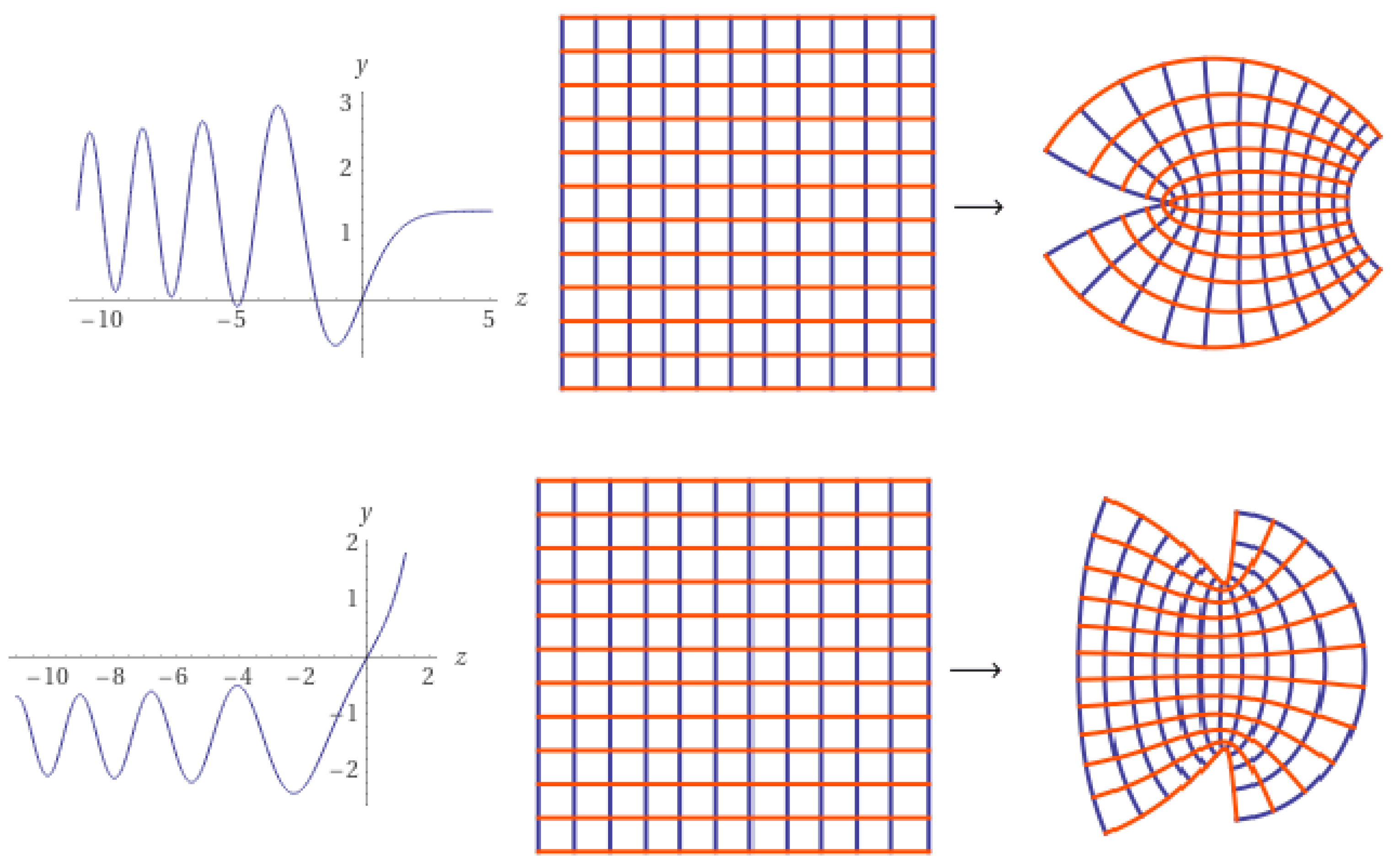
The following outcomes demonstrate some characteristics of the k−symbol Airy functions (see Figure 1).
Proposition 1.
The following outcomes are accurate for k-special functions
- where is the k-Barnes function satisfying (κ is the κ function) and is the k-modified Bessel function.
- where indicates the k-Bessel function.
- where represents the k-hypergeometric function.
2.3. K-Airy Differential Operator
Using the normalized k-Airy functions, we then define the symmetric-convex differential operator. For an analytic function normalized in the open unit disk , we have the following structure:
The following power series is produced using the convoluted operator (∗) and the normalized Airy function
By considering the above convoluted product, we define the following normalized k-Airy symmetric-convex differential operator (KASCO):
where
The m-dimensional KASCO is illustrated as follows:
Note that, under the consideration data and , this implies the Salagean differential operator [22].
2.4. Univalent Solution of the k-Wave Equation
In an effort to develop the wave equation, we suggest utilizing the parametric Koebe function. The Koebe function is an extreme function that belongs to the family of convex univalent functions. The Koebe function maps the unit disk conformally onto the complex plane with a slit along the disk . We utilize the rotate Koebe function of the structure
The operator acts on , producing the following expansion
Using the operator (2), we proceed to formulate the complex wave equation. The complex wave equation is considered in the formula
where indicates the m-iterative wave amplitude in with the convex parameter and is known as the non-linear functional of the wave under consideration owing and (normalized function in ). A unique instance is examined in [23], when and
We provide a univalent outcome to the wave equation. The univalent result is significant in wave equations (see [24,25,26,27]). The wave peaks necessarily travel faster than the troughs and ultimately reach these levels since the solutions to the wave equations are known to be erroneous for infinite layers as they are not univalent functions. The primary requirement to achieve an analytic univalent solution fulfilling the inequality is covered in the next section where Alternatively, the answer is a complex domain with a limited rotation function. In this instance, the gradients continue to increase, but eventually these effects start to occur, slowing this expansion. The precise behavior of the solution in , which cannot be predicted from the wave equation, depends on the form of the dissipation components that are taken into account.
3. Results and Discussion
This section describes our findings for the univalent solution of Equation (3) for various hypotheses concerning .
Proposition 2.
Proof.
The normalization formula of yields and Replacing by in the inequality (4), we get
Different conditions for to be univalently solvable are shown in the following outcomes.
Proposition 3.
Proof.
Assume that (7) is a true inequality. Formulate an admissible function , as follows:
Extra conditions on to be univalent. The following outcome is a relation between and in Equation (3).
Proposition 4.
Proof.
Let and Formulate the function as follows:
Clearly, is analytic in Integrating both sides, we get
Consequently, we have
Therefore, a calculation gives that
where
A calculation yields that
By virtue of the assumption, we have
where The next step is to prove that or
Consequently, we obtain that is a univalent solution of Equation (3) in □
Some unique examples of Proposition 4 are as follows:
Corollary 1.
If
then is a univalent solution.
Proof.
By putting in Proposition 4, we have the result. Note that this result is sharp when
where
□
By Corollary 1, we have
Corollary 2.
If
where
then is a univalent solution.
The concluding remarks are presented below.
Remark 1.
- Solutions that are periodic exist because is an integer with Keobe function. Since individual modes do not necessarily have to be periodic, this restriction is not required. Instead, the value of t will be determined by the boundary conditions. Furthermore, it is asserted that without sacrificing generality, and special emphasis is given to solutions that behave as . The waves in the direction of positive t are attenuated in this way. The form of the waves traveling in the direction of negative t is the same (symmetric sense).
- The way in which the concept is developed here readily lends itself to many generalizations. This represents an intriguing situation when the height of the top border varies along the direction of propagation. The normalized analytic function is seen as a function of to obtain the normalized univalent solution in the complex model under study.
- It may be anticipated that a waveguide with slowly changing characteristics will not differ greatly from a waveguide with a constant cross-section based on fundamental principles. The structure of the modes may be used to identify a normalized waveguide with a univalent function. The ideal ground conductivity is now standardized to a value that is very near to unity.
4. Conclusions
A symmetric-convex differential formula of normalized Airy functions in the open unit disk was developed. This equation was taken into account as a differential operator working on a class of normalized analytic functions. The proposed operator (KASCO) was shown to be a solution to a wave equation in the following phase of this inquiry. We provided the necessary requirements for KASCO to be a univalent solution because we sought to analyze the geometric shape of the solution (symmetry and convexity). Based on the theory of the wave equation of a complex variable, the univalent solution is a particularly delicate property. Based on the theory of geometric functions, this characteristic leads to several geometric presentations for the solution.
Author Contributions
Conceptualization, R.W.I. and S.B.H.; methodology, R.W.I.; software, S.B.H.; validation, R.W.I. and S.B.H.; formal analysis, R.W.I.; investigation, S.B.H.; writing—original draft preparation, R.W.I. and S.B.H.; funding acquisition, S.B.H. All authors have read and agreed to the published version of the manuscript.
Funding
This research was funded by Ajman University Fund: 2022-IRG-HBS-8.
Institutional Review Board Statement
Not applicable.
Informed Consent Statement
Not applicable.
Data Availability Statement
Not applicable.
Conflicts of Interest
The authors declare no conflict of interest.
References
- Diaz, R.; Pariguan, E. On hypergeometric functions and Pochhammer k-symbol. Divulg. Math. 2007, 15, 179–192. [Google Scholar]
- Diaz, R.; Pariguan, E. Feynman-Jackson integrals. J. Nonlinear Math. Phys. 2006, 13, 365–376. [Google Scholar] [CrossRef] [Green Version]
- Karwowski, J.; Witek, A.H. Biconfluent Heun equation in quantum chemistry: Harmonium and related systems. Theor. Chem. Acc. 2014, 133, 1494. [Google Scholar] [CrossRef] [Green Version]
- Lackner, M.; Lackner, M. On the likelihood of single-peaked preferences. Soc. Choice Welf. 2017, 48, 717–745. [Google Scholar] [CrossRef] [Green Version]
- Kilbas, A.A.; Srivastava, H.M.; Trujillo, J.J. Theory and Applications of Fractional Differential Equations; North-Holland Mathematical Studies; Elsevier (North-Holland) Science Publishers: Amsterdam, The Netherlands; London, UK; New York, NY, USA, 2006; Volume 204. [Google Scholar]
- Agarwal, P.; Chand, M.; Baleanu, D.; O’Regan, D.; Shilpi, J. On the solutions of certain fractional kinetic equations involving k-Mittag-Leffler function. Adv. Differ. Equ. 2018, 1, 249. [Google Scholar] [CrossRef]
- Set, E.; Tomar, M.; Sarikaya, M.Z. On generalized Grüss type inequalities for k-fractional integrals. Appl. Math. Comput. 2015, 269, 29–34. [Google Scholar] [CrossRef]
- Diaz, R.; Teruel, C. q, k-generalized gamma and beta functions. J. Nonlinear Math. Phys. 2005, 12, 118–134. [Google Scholar] [CrossRef] [Green Version]
- Diaz, R.; Pariguan, E. On the Gaussian q-distribution. J. Math. Anal. Appl. 2015, 358, 1–9. [Google Scholar] [CrossRef] [Green Version]
- Mondal, S.R.; Mohamed, S.A. Differential equation and inequalities of the generalized k-Bessel functions. J. Inequalities Appl. 2018, 2018, 175. [Google Scholar] [CrossRef] [PubMed] [Green Version]
- Seoudy, T.M. Some subclasses of univalent functions associated with k-Ruscheweyh derivative operator. Ukrains’ kyi Matematychnyi Zhurnal 2022, 74, 122–136. [Google Scholar] [CrossRef]
- Aktas, I. On monotonic and logarithmic concavity properties of generalized k-Bessel function. Hacet. J. Math. Stat. 2021, 50, 180–187. [Google Scholar] [CrossRef]
- Guptaa, A.; Pariharb, C.L. Siago’s K-Fractional Calculus Operators. Malaya J. Mat. 2017, 5, 494–504. [Google Scholar]
- Olivier, V.; Soares, M. Airy Functions and Applications to Physics; World Scientific Publishing Company: Singapore, 2010. [Google Scholar]
- Valle’e, O. Some Integrals Involving Airy Functions and Volterra μ-Functions. Integral Transform. Spec. Funct. 2002, 13, 403–408. [Google Scholar] [CrossRef]
- AAnikin, A.Y.; Dobrokhotov, S.Y.; Nazaikinskii, V.E.E.; Tsvetkova, A.V. Uniform asymptotic solution in the form of an Airy function for semiclassical bound states in one-dimensional and radially symmetric problems. Theor. Math. Phys. 2019, 201, 1742–1770. [Google Scholar] [CrossRef]
- Minin, O.V.; Minin, I.V. Formation of a Photon Hook by a Symmetric Particle in a Structured Light Beam. In The Photonic Hook; Springer: Cham, Switzerland, 2021; pp. 23–37. [Google Scholar]
- Chen, J.; Gao, L.; Jin, Y.; Reno, J.L.; Kumar, S. High-intensity and low-divergence THz laser with 1D autofocusing symmetric Airy beams. Optics Express 2019, 27, 22877–22889. [Google Scholar] [CrossRef] [PubMed]
- Suarez, R.A.; Gesualdi, M.R. Propagation of Airy beams with ballistic trajectory passing through the Fourier transformation system. Optik 2020, 207, 163764. [Google Scholar] [CrossRef] [Green Version]
- Len, M. Precise dispersive estimates for the wave equation inside cylindrical convex domains. Proc. Am. Math. Soc. 2022, 150, 12. [Google Scholar] [CrossRef]
- Indenbom, M.V. Method for Calculation of the Interaction of Elements in a Large Convex Quasi-Periodic Phased Antenna Array. J. Commun. Technol. Electron. 2022, 67, 616–626. [Google Scholar] [CrossRef]
- Salagean, G.S. Subclasses of univalent functions. In Complex Analysis-Fifth Romanian-Finnish Seminar; Springer: Berlin/Heidelberg, Germany, 1983; pp. 362–372. [Google Scholar]
- Wait, J.R. Two-dimensional treatment of mode theory of the propagation of VLF radio waves. Radio Sci. D 1964, 68, 81–94. [Google Scholar] [CrossRef]
- Broer, L.J.F.; Sarluy, P.H.A. On simple waves in non-linear dielectric media. Physica 1964, 30, 1421–1432. [Google Scholar] [CrossRef]
- Ibrahim, R.W.; Meshram, C.; Hadid, S.B.; Momani, S. Analytic solutions of the generalized water wave dynamical equations based on time-space symmetric differential operator. J. Ocean. Eng. Sci. 2020, 5, 186–195. [Google Scholar] [CrossRef]
- Ibrahim, R.W.; Baleanu, D. Symmetry breaking of a time-2D space fractional wave equation in a complex domain. Axioms 2021, 10, 141. [Google Scholar] [CrossRef]
- Ibrahim, R.W.; Elobaid, R.M.; Obaiys, S.J. Generalized Briot-Bouquet differential equation based on new differential operator with complex connections. Axioms 2020, 9, 42. [Google Scholar] [CrossRef] [Green Version]
- Kaplan, W. Close-to-convex schlicht functions. Mich. Math. J. 1952, 1, 169–185. [Google Scholar] [CrossRef]
- Miller, S.S.; Mocanu, P.T. Second order differential inequalities in the complex plane. J. Math. Anal. Appl. 1978, 65, 289–305. [Google Scholar] [CrossRef]
Figure 1.
The graph of the normalized Airy functions , respectively.

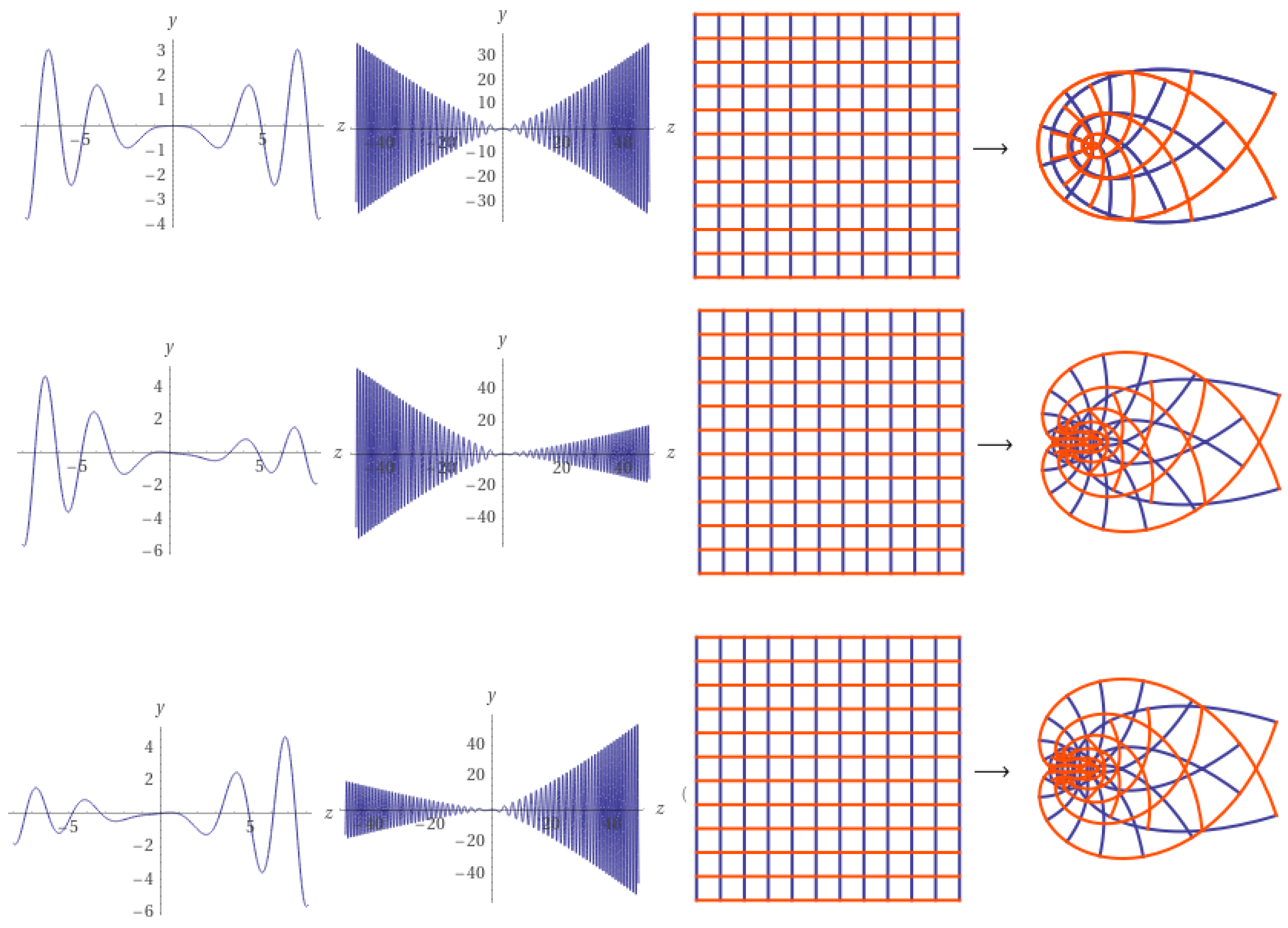
Figure 2.
The graph of KASCO, when accordingly.

Publisher’s Note: MDPI stays neutral with regard to jurisdictional claims in published maps and institutional affiliations. |
© 2022 by the authors. Licensee MDPI, Basel, Switzerland. This article is an open access article distributed under the terms and conditions of the Creative Commons Attribution (CC BY) license (https://creativecommons.org/licenses/by/4.0/).
Share and Cite
MDPI and ACS Style
Hadid, S.B.; Ibrahim, R.W. Geometric Study of 2D-Wave Equations in View of K-Symbol Airy Functions. Axioms 2022, 11, 590. https://doi.org/10.3390/axioms11110590
AMA Style
Hadid SB, Ibrahim RW. Geometric Study of 2D-Wave Equations in View of K-Symbol Airy Functions. Axioms. 2022; 11(11):590. https://doi.org/10.3390/axioms11110590
Chicago/Turabian StyleHadid, Samir B., and Rabha W. Ibrahim. 2022. "Geometric Study of 2D-Wave Equations in View of K-Symbol Airy Functions" Axioms 11, no. 11: 590. https://doi.org/10.3390/axioms11110590
Note that from the first issue of 2016, this journal uses article numbers instead of page numbers. See further details here.