
A Discrete Linear-Exponential Model: Synthesis and Analysis with Inference to Model Extreme Count Data


1
Department of Mathematics, College of Science and Humanities in Al-Kharj, Prince Sattam bin Abdulaziz University, Al-Kharj 11942, Saudi Arabia
2
Department of Mathematics, Faculty of Science, Mansoura University, Mansoura 35516, Egypt
Axioms 2022, 11(10), 531; https://doi.org/10.3390/axioms11100531
Submission received: 2 September 2022
/
Revised: 22 September 2022
/
Accepted: 30 September 2022
/
Published: 4 October 2022
Abstract
:In this article, a novel probability discrete model is introduced for modeling overdispersed count data. Some relevant statistical and reliability properties including the probability mass function, hazard rate and its reversed function, moments, index of dispersion, mean active life, mean inactive life, and order statistics, are derived in-detail. These statistical properties are expressed in closed forms. The new model can be used to discuss right-skewed data with heavy tails. Moreover, its hazard rate function can be utilized to model the phenomena with a monotonically increasing failure rate shape. Different estimation approaches are listed to get the best estimator for modeling and reading the count data. A comprehensive comparison among techniques is performed in the case of simulated data. Finally, four real data sets are analyzed to prove the ability and notability of the new discrete model.
1. Introduction
Data modeling in recent years has been very complicated due to the huge number of data sets which have been generated from different fields over time, especially, in engineering, medical, ecology, and renewable energy. The principal problem is when the data are suffering from overdispersion with different kinds of kurtosis including leptokurtic- or platykurtic-shaped. Therefore, it is important to model and analyze such data by utilizing a flexible probability distribution. Thus, several continuous probability models have been introduced and discussed in the statistical literature for this purpose. In several cases, the data need to be recorded on a discrete scale rather than on a continuous analogue. Due to the previous reason, the discretization of existing continuous distributions has received a wide attention because of the count data generated from various areas becoming more complex day-by-day. So, for modeling these count data, we need discrete probability models that are best suited for analytical studies of this multidimensional and complex phenomena. Many discrete distributions have been proposed and studied in detail such as the discrete Rayleigh (see Roy [1]), discrete Pareto (see Krishna and Pundir [2]), discrete exponential generalized-G family (see Eliwa et al. [3]), discrete Lindley (see Gommez-Déniz and Calderin-Ojeda [4]), discrete generalized exponentiated type two (see Nekoukhou et al. [5]), discrete exponentiated Weibull (see Nekoukhou and Bidram [6]), discrete Lindley-II (DLi-II) (see Hussain et al. [7]), discrete Burr XII (see Para and Jan [8]), discrete Gompertz-G class (see Eliwa el al. [9]), discrete exponentiated Lindley (see El-morshedy et al. [10]), discrete generalized Burr-Hatke (see Yousof et al. [11]), discrete Rayleigh-G family (see Ibrahim et al. [12]), binomial new Poisson-weighted exponential model (see Al-Bossly and Eliwa [13]), among others. Although there are a number of discrete models in the literature, there is still a lot of space left to propose a new discretized model that is suitable under various conditions.
Recently, Sah [14] introduced a novel one-parameter linear-exponential (NLE) distribution. The NLE distribution was based on the product of a linear function and an exponential function with a single parameter . The cumulative distribution function (CDF) of the NLE model could be expressed as
where is a scale parameter. In this paper, a discrete analogue of the NLE model is presented under the abbreviation NDsLE. The nice feature of reporting the NDsLE model is that it stands with a single parameter which is to be listed so as to give a better alternative for some discrete distributions and to create another platform for researchers working on probability distribution theory. Other interesting features for the NDsLE model can be listed as follows:
- Its distributional statistics can be expressed in explicit terms.
- It can be used to model positively skewed count data.
- It can be utilized to discuss overdispersed count data.
- It can be applied to study count data which have a monotonically increasing hazard rate function (HRF).
- It can be used as a statistical tool to model extreme count data.
The rest of the paper is organized as follows, In Section 2, we introduce the NDsLE distribution. Various distributional statistics are derived in Section 3. In Section 4, the NDsLE parameter is estimated by using various techniques including maximum likelihood, proportion, moments, least squares, weighted least squares, and Cramér–von Mises criterion to get the best estimator for modeling data. A simulation study is presented in Section 5. Four real data sets are analyzed to show the flexibility of the NDsLE distribution in Section 6. Finally, Section 7 provides some conclusions.
2. The NDsLE Distribution: Mathematical Synthesis
Starting with (1) and utilizing the discretization concepts, the CDF of the NDsLE distribution can be expressed as
where and . The survival function corresponding to (2) can be proposed as
The probability mass function (PMF) can be formulated as
where the PMF of any discrete random variable (RV) can be derived as
where is a vector of parameters. The PMF in (4) is log-concave, where is a decreasing function in x for all values of the NDsLE parameter. Depending on (4) and (3), the HRF can be derived as
where whereas the reversed HRF (RHRF) can be presented as
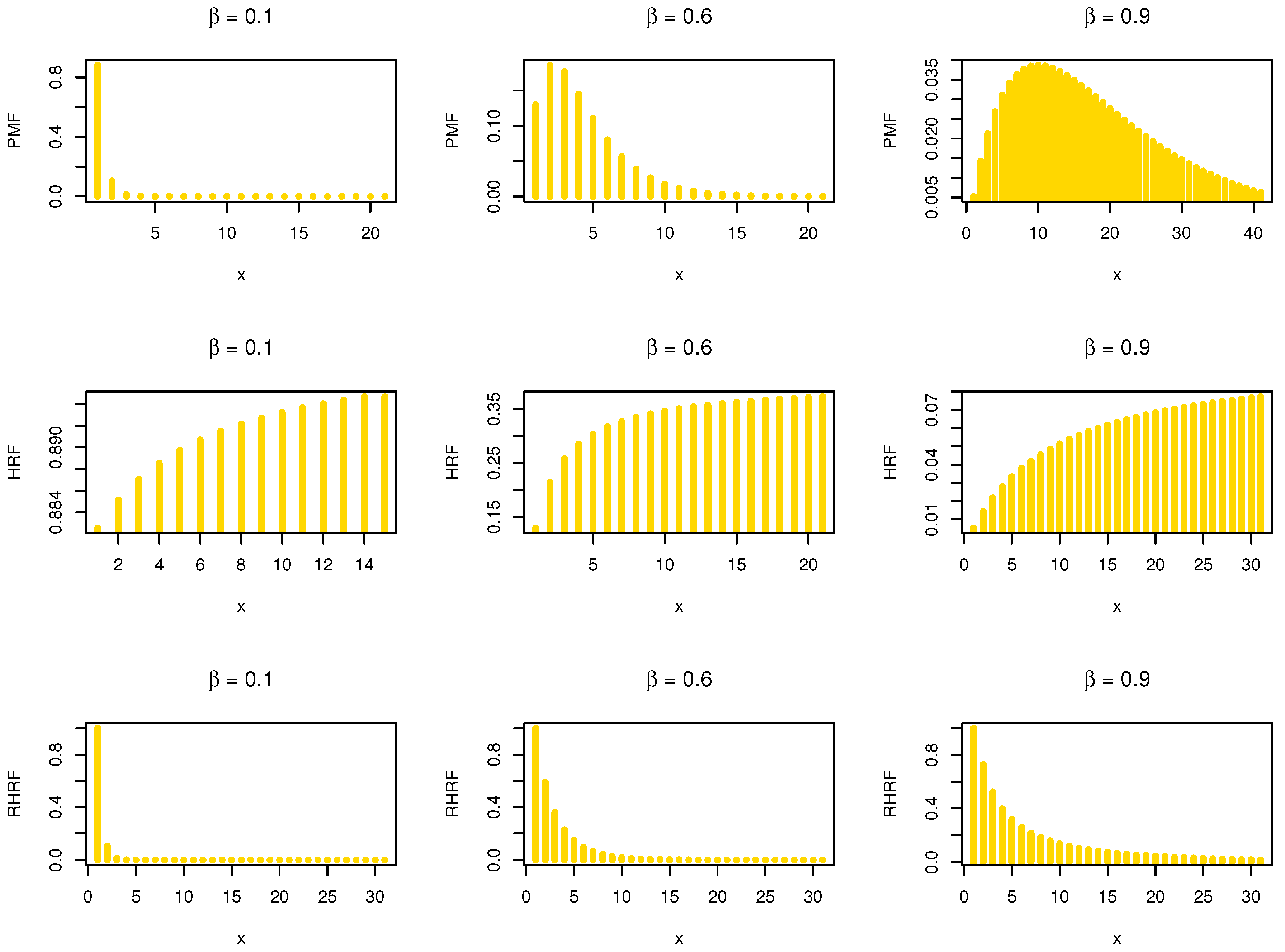
where . In Figure 1, we give some , and plots of the NDsLE model under some selected parameter values.
Based on Figure 1, it is noted that the of the NDsLE model is unimodal, and it can be used as a probability tool to model asymmetric data. Moreover, the NDsLE model is a proper approach for modeling some phenomena which have increasing HRF or decreasing RHRF. Suppose Y and Z are two independent NDsLE RVs with parameters and , respectively. Then, the HRF of min can be formulated as
then
The extra term arises because in the discrete form, . Since the HRF of the two RVs Y and Z is increasing, then the HRF of min is also increasing. Similarly, the HRF of max can be expressed as
3. Main Statistical and Reliability Properties
3.1. Ordinary Moments and Descriptive Statistics
Let X be a non-negative RV, where X∼NDsLE(), then the rth moments can be expressed as
where Hurwitzlerchphi represents the Hurwitz–Lerch transcendental function which can be proposed in the form . Setting in (8), the first four moments of the RV X can be derived in closed forms as
and
According to the previous four moments, the variance “”, skewness “”, and kurtosis “” can be expressed in closed forms where
and
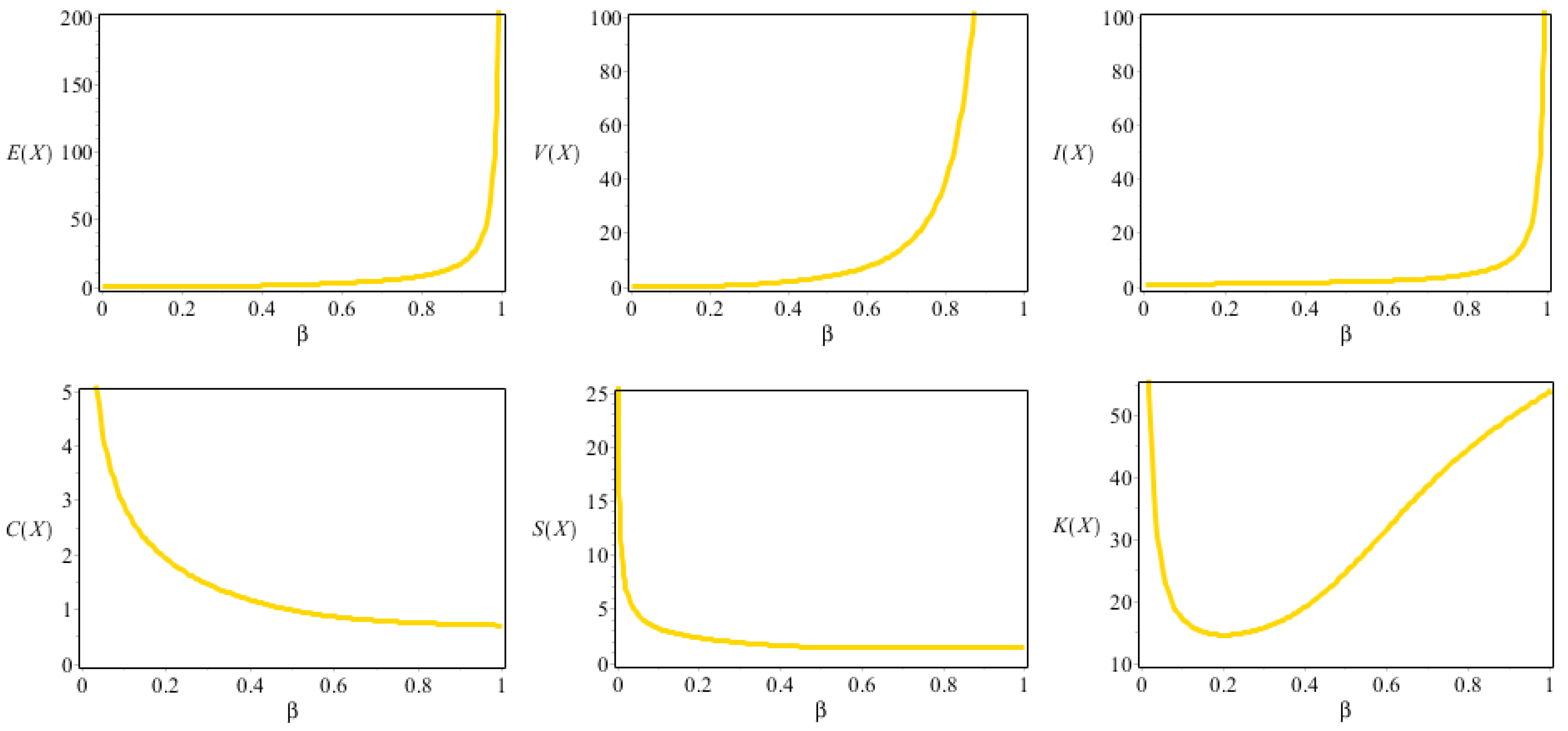
The index of dispersion, say , is defined as the to ratio; it indicates whether a certain model is suitable for under or overdispersed data sets. If , the model is under- (over)dispersed. Further, the coefficient of variation, say , is reported. The can be formulated in closed expression as
Table 1 lists some numerical results of some descriptive statistics (DS) for the NDsLE model for different values of the parameter .
3.2. Mean Active and Inactive Life Measures
To study the aging behavior of a component, several reliability measures have been defined in the survival analysis (SA) literature. One of them is called the mean active life (MAL). The MAL is a helpful reliability tool to analyze the burn-in and maintenance policies. In the discrete setting, the MAL can be defined as for and . Assume the RV X∼NDsLE(), then the MAL can be formulated as
where
Another reliability concept of interest in SA is the mean inactive life (MIAL), which measures the time elapsed since the failure of X given that the component has failed some time before i. The MIAL, say , is defined as for and . Let X∼NDsLE(), then the MIAL can be expressed as
where
For we get . Let X be a NDsLE RV, then the CDF can be proposed by the MIAL as
where and The mean of the NDsLE distribution can be expressed as
The RHRF and the MIAL are related as
3.3. Order Statistics (ORSS) and L-Moment (L-M) Statistics
Let , be a random sample (RS) from the NDsLE distribution, and let be their corresponding ORSS. Then, the CDF of the ith ORSS is
where and represents the CDF of the exponentiated NDsLE model with power parameter Further, the corresponding PMF of the ith ORSS can be expressed as
where . The moments of is
4. Estimation Approaches
4.1. Maximum Likelihood Estimation (MLE)
In this section, we list the MLEs of the NDsLE parameter. Let be an RS of size p from the NDsLE model. The log-likelihood function (L) can be formulated as
By differentiating (13) with respect to the parameter , we get the normal nonlinear likelihood equation as follows
The resulted equation cannot be solved analytically. Thus, an iterative procedure such as the Newton–Raphson method is required to solve it numerically.
4.2. Proportion Estimation (ProE)
Assume is an RS of size p from the NDsLE model. We define an indicator as follows
Let stand for the number of zeros in the RS. Using the CDF of the NDsLE model as well as (14), we get So, the parameter is estimated by solving the following equation
where the of is an unbiased and consistent estimator. In some cases, we could not get the zeros in the RS. Thus, we replace zeros by ones or by any observation inside the sample to get the estimator.
4.3. Moment’s Estimation (MoE)
Let be an RS of size p from the NDsLE distribution. Based on the approach of moments for estimating the parameter , we can derive the estimator by solving the following equation
with respect to . A symbolic program should be utilized to solve (15) numerically according to data observations .
4.4. Least Squares and Weighted Least Squares Estimations
Let be the ORSS of the RS of size p from the NDsLE model. The least squares estimator, say LSE, of the NDsLE parameter can be derived by minimizing
with respect to , while the weighted LSE, say WLSE, of the NDsLE parameter can be proposed by minimizing
also with respect to .
4.5. Cramér–Von Mises Minimum Distance (MD) Estimation
Cramér–von Mises estimator, say CVME, is a type of MD estimator and has less bias than the other MD estimators. Assume is the ORSS of the RS of size p from the NDsLE distribution. Then, the CVME of the NDsLE parameter is listed by minimizing
with respect to .
5. Simulations: Comparing Various Estimators (CVE)
A general form to generate an RV X from the NDsLE model is to first generate the value Z from the NLE distribution, and then to discretize this value to get where is the largest integer less than or equal to . In this section, we assess the performance of the MLE, MoE, ProE, LSE, WLSE, and CVME estimators with respect to sample size p using R software. For CVE, Markov chain Monte Carlo simulations were performed based on various schemes. The assessment was based on a simulation study:
- 1
- Generate samples of different sizes “” from the NDsLE model as follows
- scheme I: |
- scheme II: |
- scheme III: |,
- 2
- Compute the MLE, MoE, ProE, LSE, WLSE, and CVME for the samples, say for
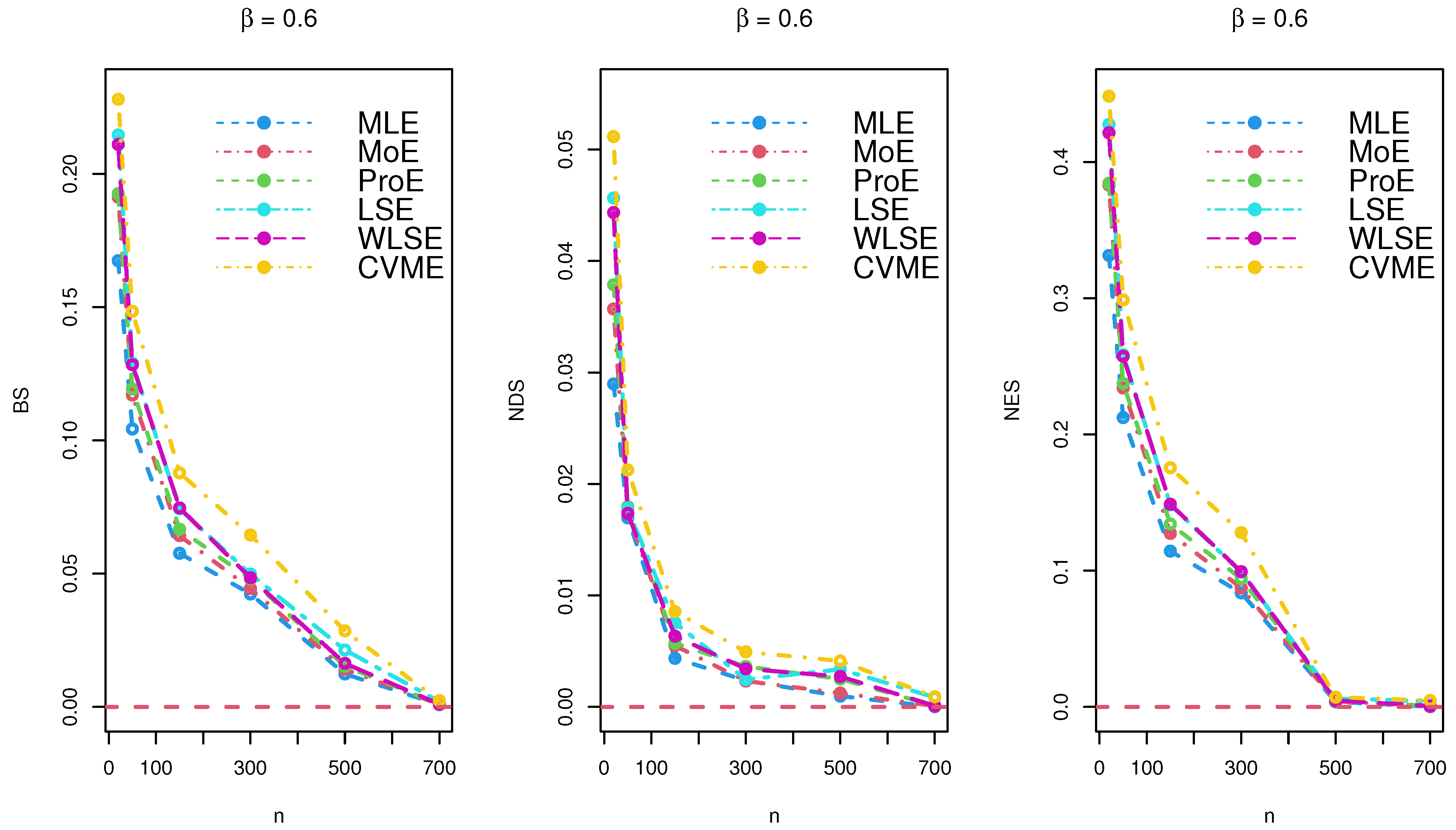
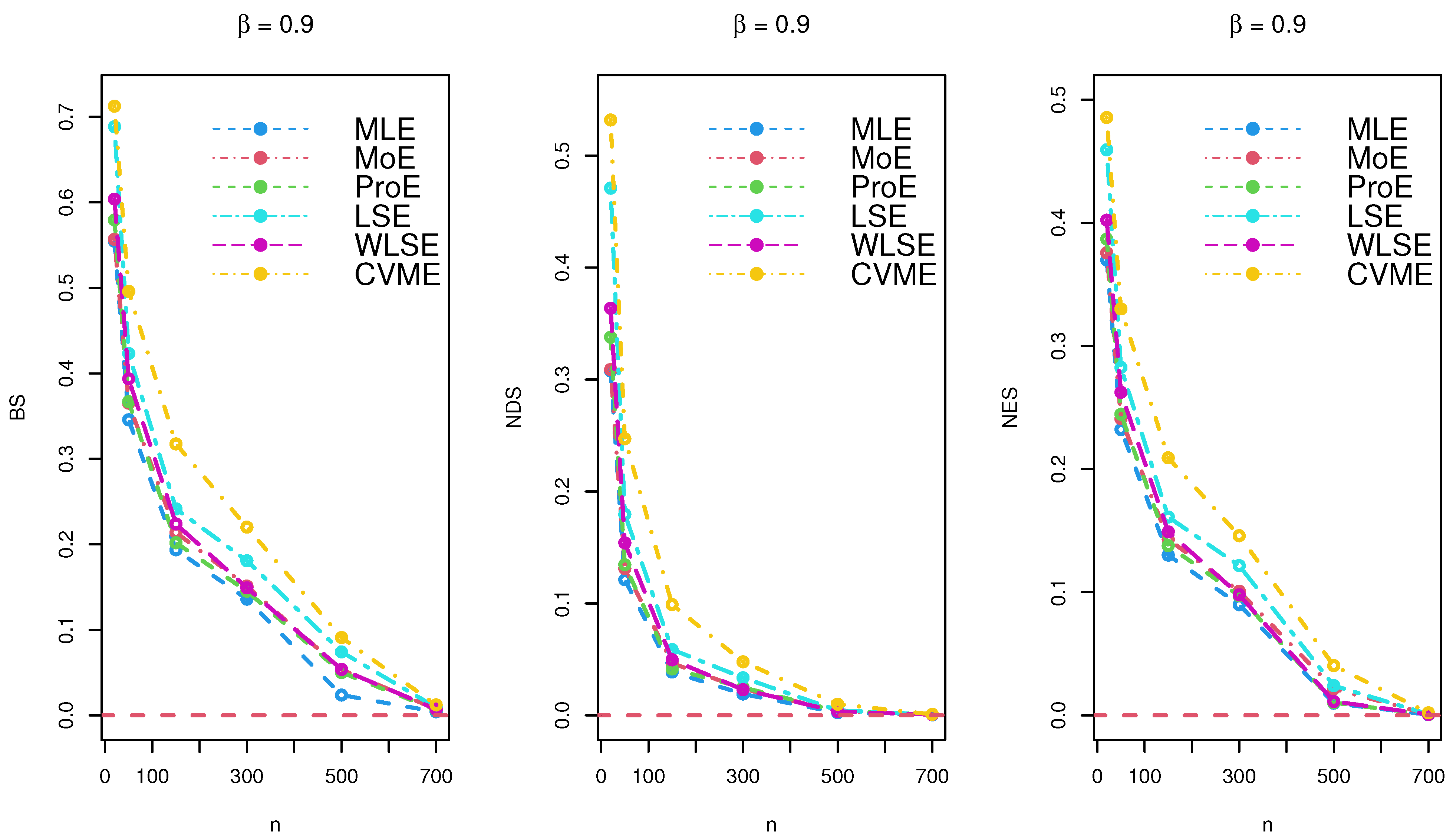
We calculated the bias “BS”, mean squared errors (NDS), mean relative errors (NES) for samples as
The results of the simulations are listed in Table 2, Table 3 and Table 4 and provided via Figure 3, Figure 4 and Figure 5. Based on the reported tables and figures, the BS approached to zero when the sample size p increased. Similarly, the NDS and NES of the parameter approached zero when p increased. These results revealed the unbiasedness, efficiency, consistency properties of the MLE, MoE, ProE, LSE, WLSE, and CVME estimators. Thus, we can conclude that all estimation techniques worked quite well under different sizes of samples.
6. A Comparative Study to Model Extreme and Outliers Observations
In this Section, we test the fitting capability of the NDsLE distribution. The fitting of the distributions were compared utilizing some well-known statistical measures, namely, , the Akaike information criterion (A), the correct Akaike information criterion (CA), the Hannan–Quinn information criterion (H), and the Kolmogorov–Smirnov (K–S) test as well as the chi-square () test with its degree of freedom (DF), and the associated p-value (PV). The competitive models (CMs) are provided in Table 5.
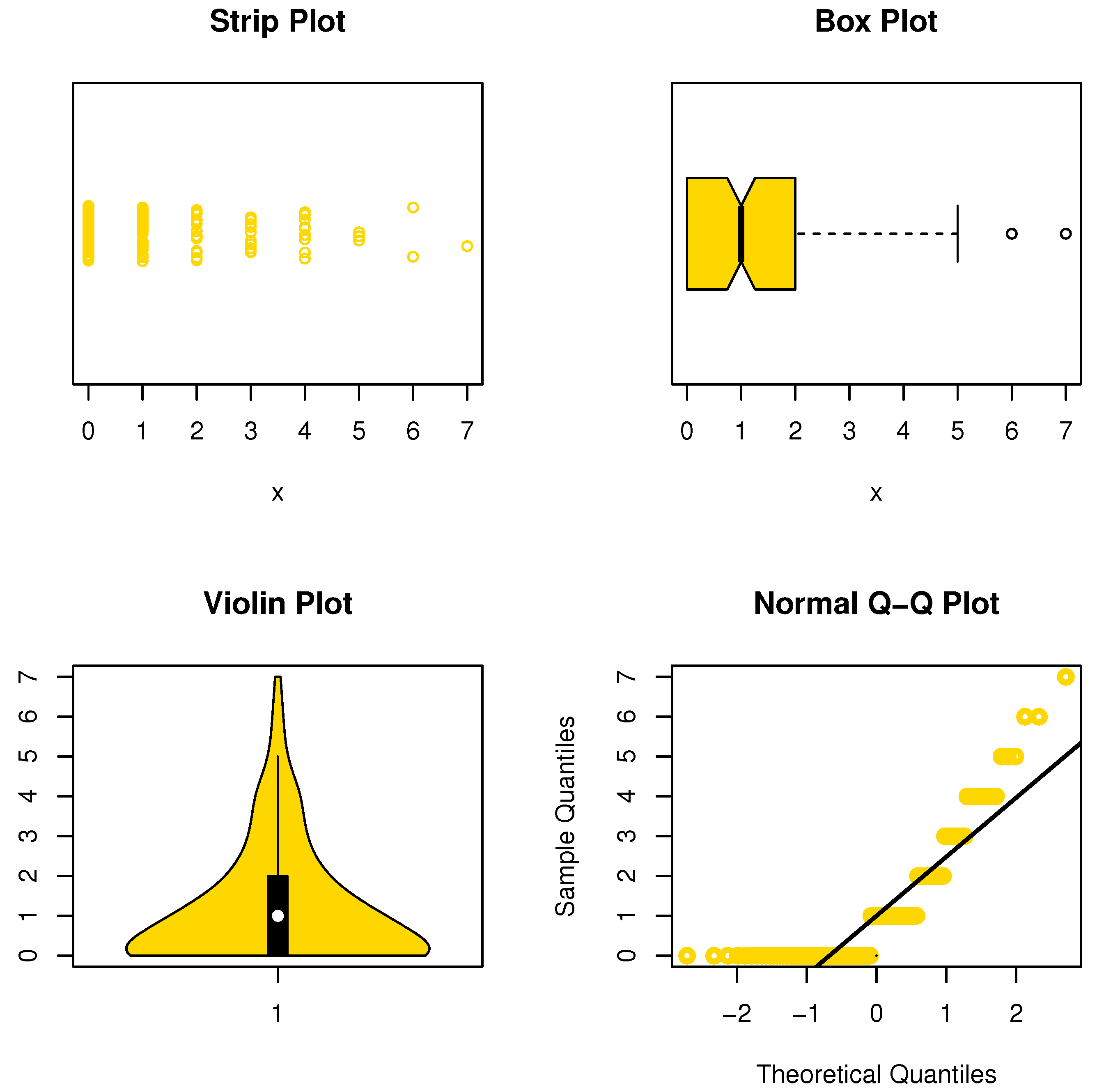
6.1. Data Set I
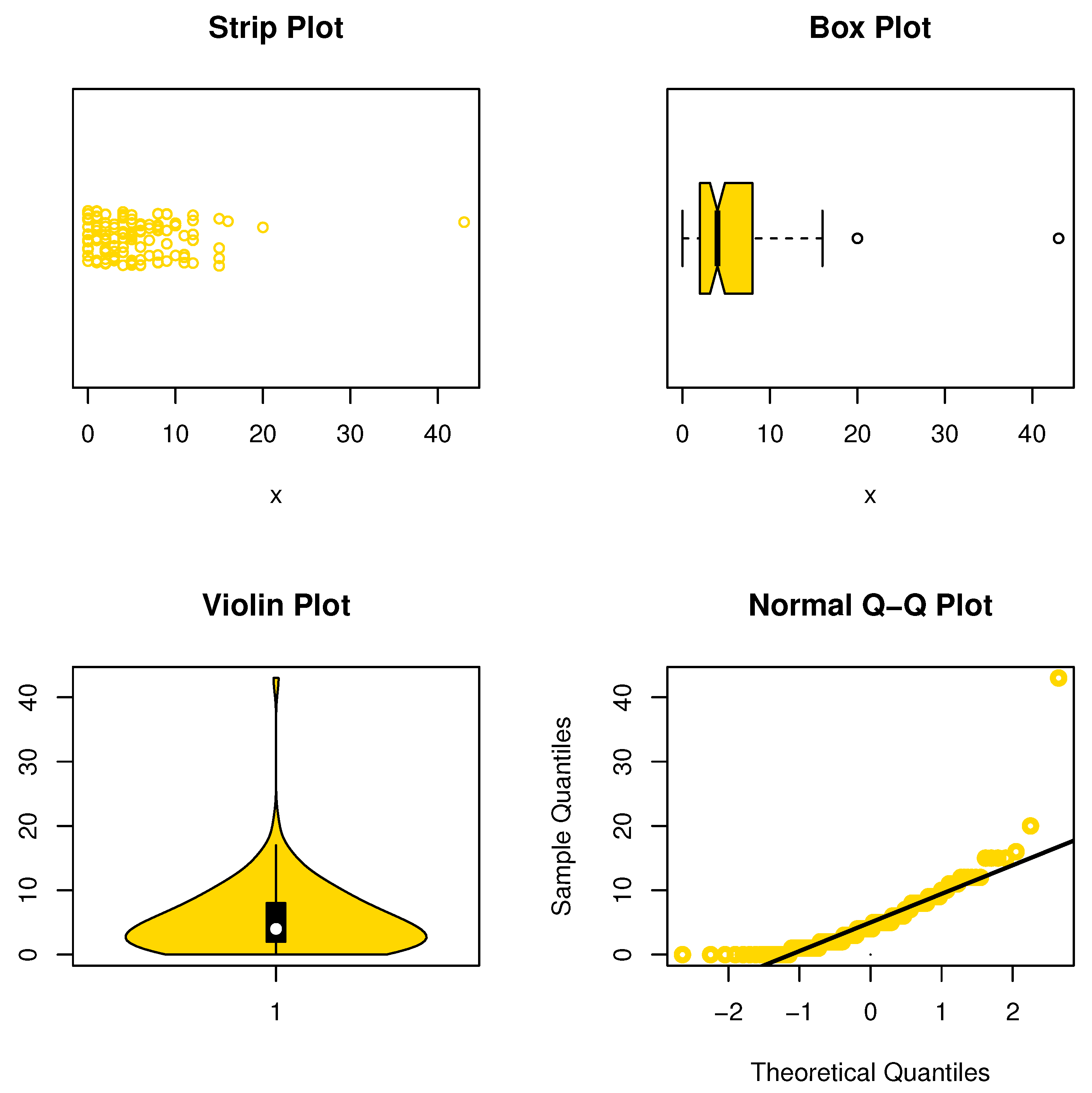
This data set represents the number of European red mites on apple leaves (see Chakraborty and Chakravarty [20]). The initial mass shape is reported using nonparametric approaches such as strip, box, violin, and QQ plots in Figure 6. It is noted that the data are asymmetric and some extreme observations are found. Table 4 reports the MLEs with its standard errors (Std-er), and confidence interval (C.I) for the NDsLE parameter and other CMs. Further, the goodness-of-fit (GOF) measures as well as expected (observed) frequency, say EF (OF), have been listed in the same Table.
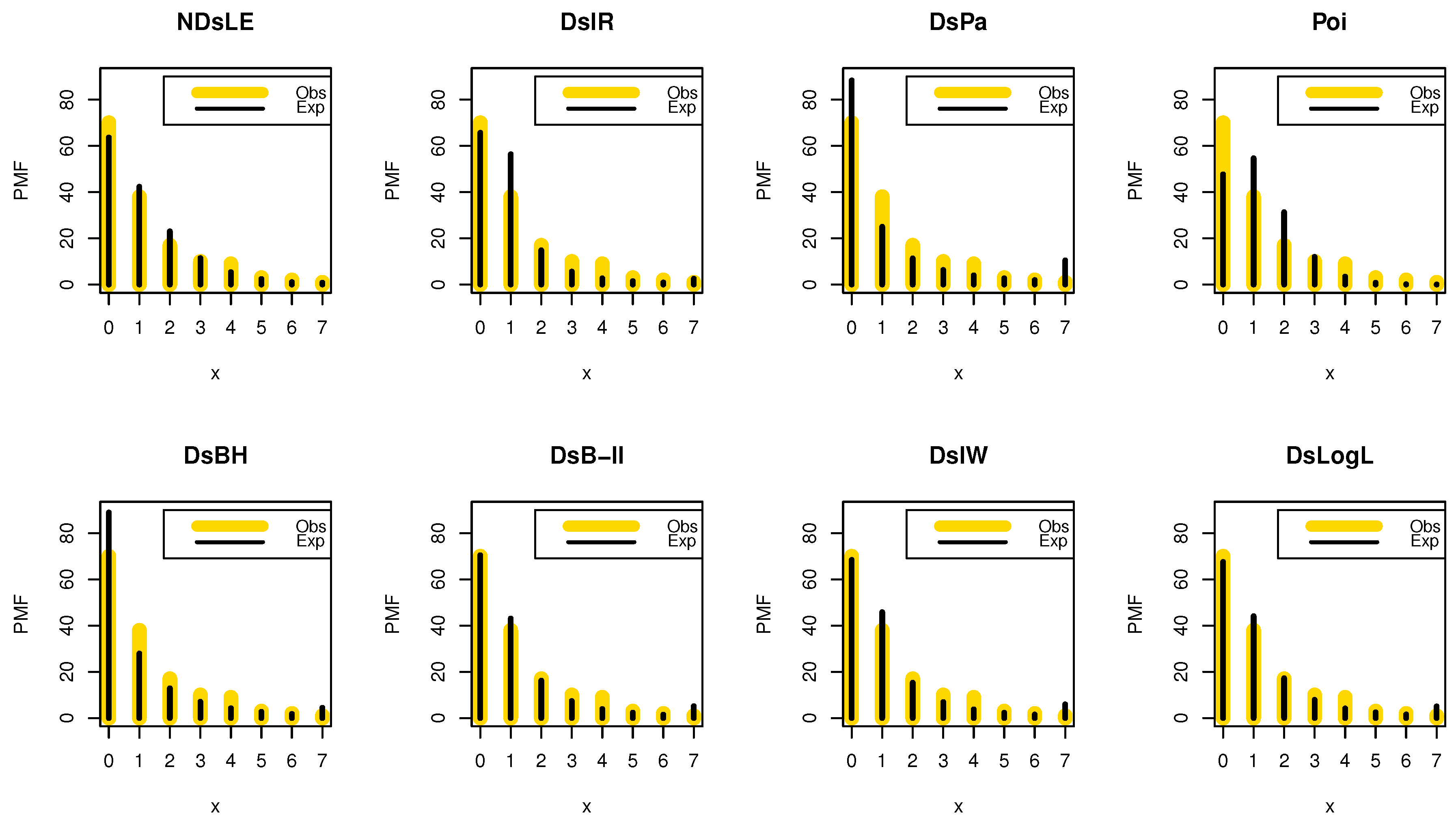
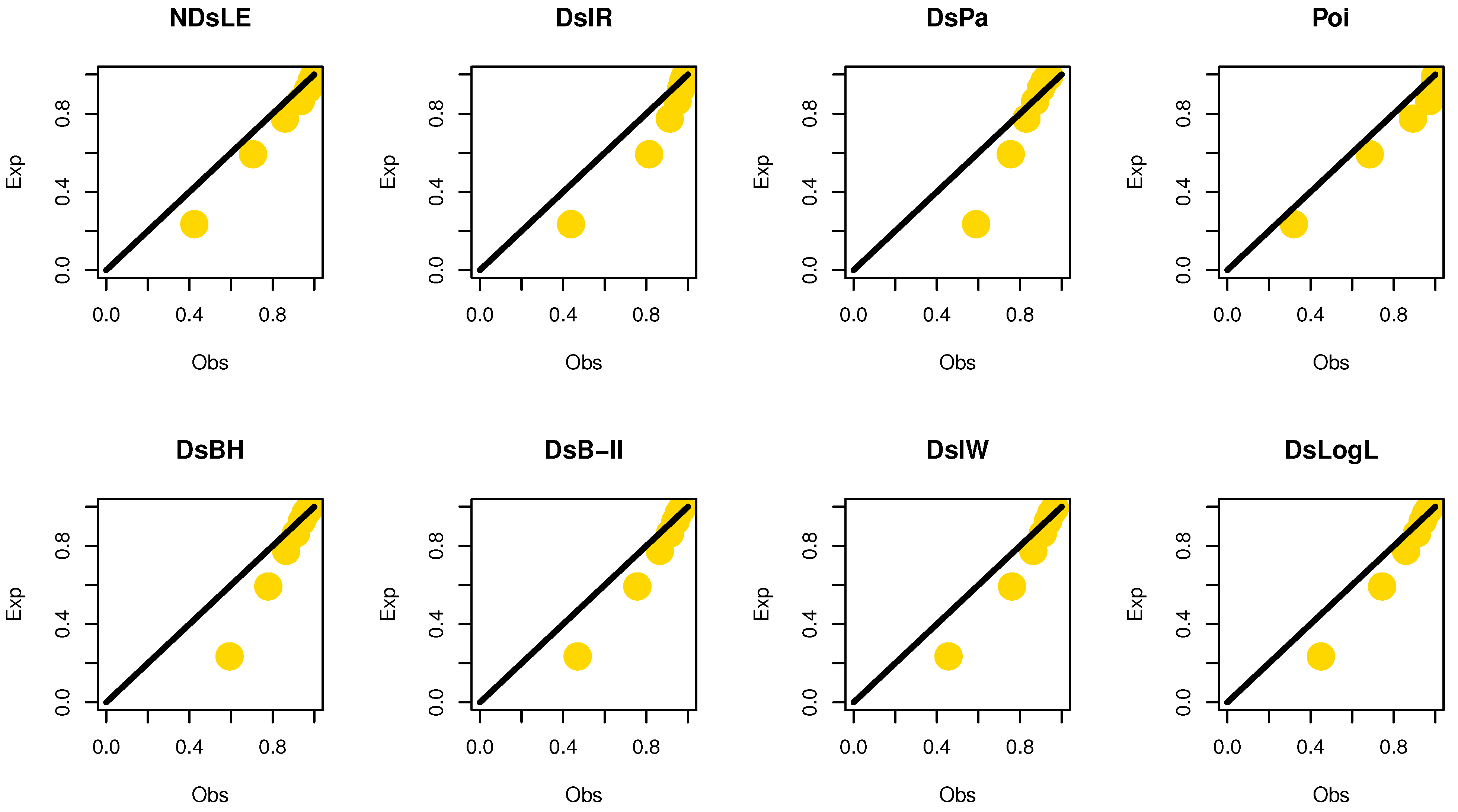
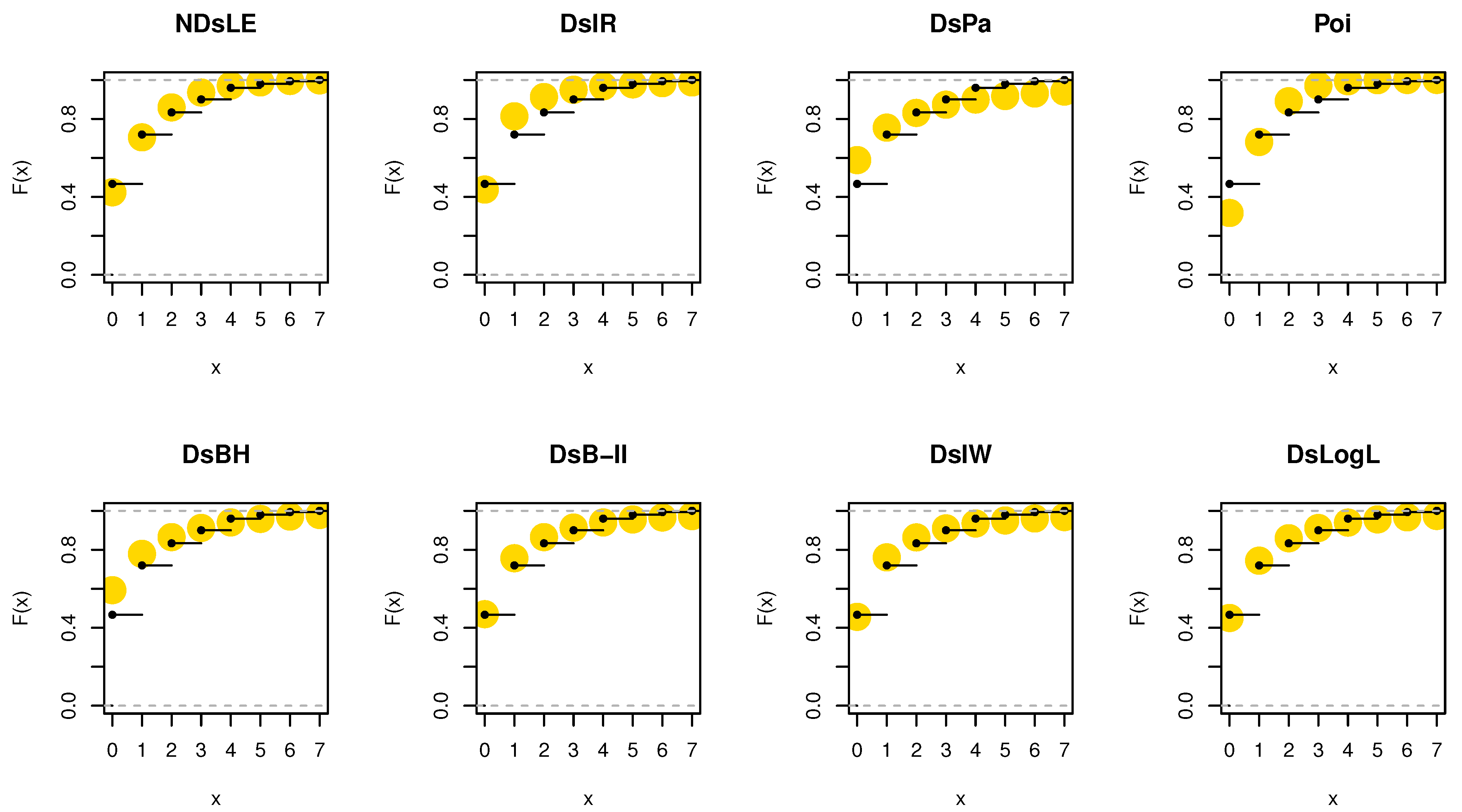
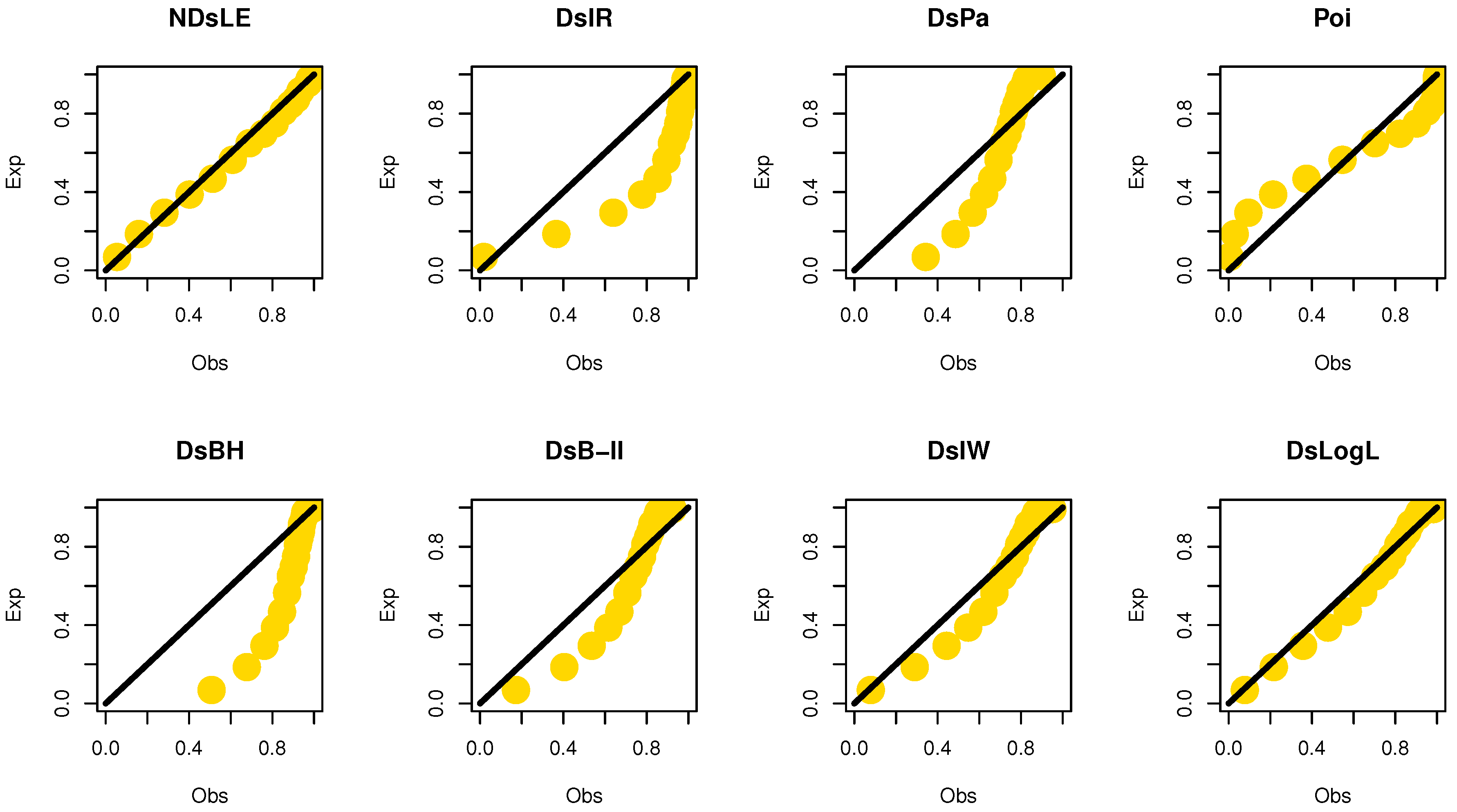
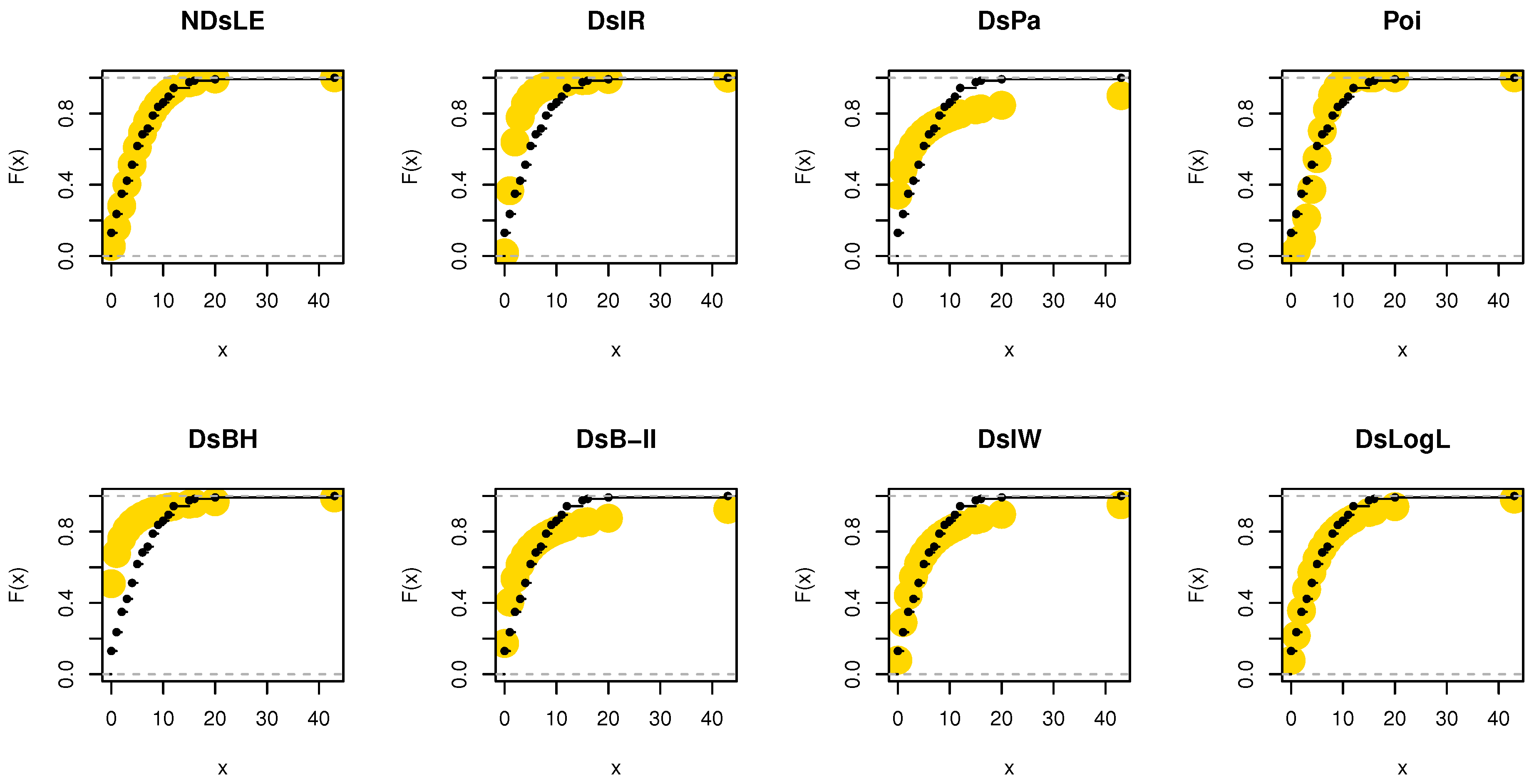
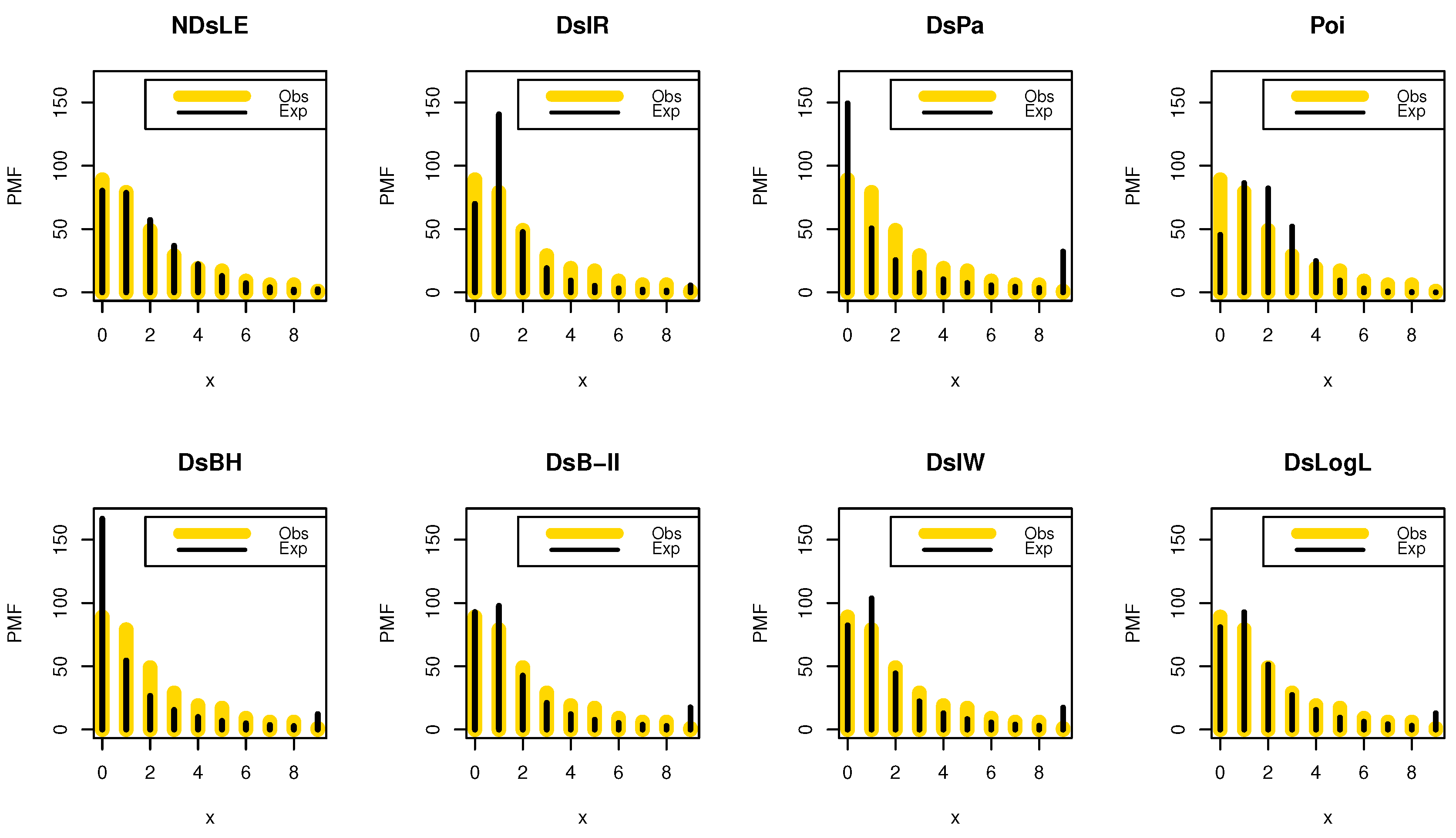
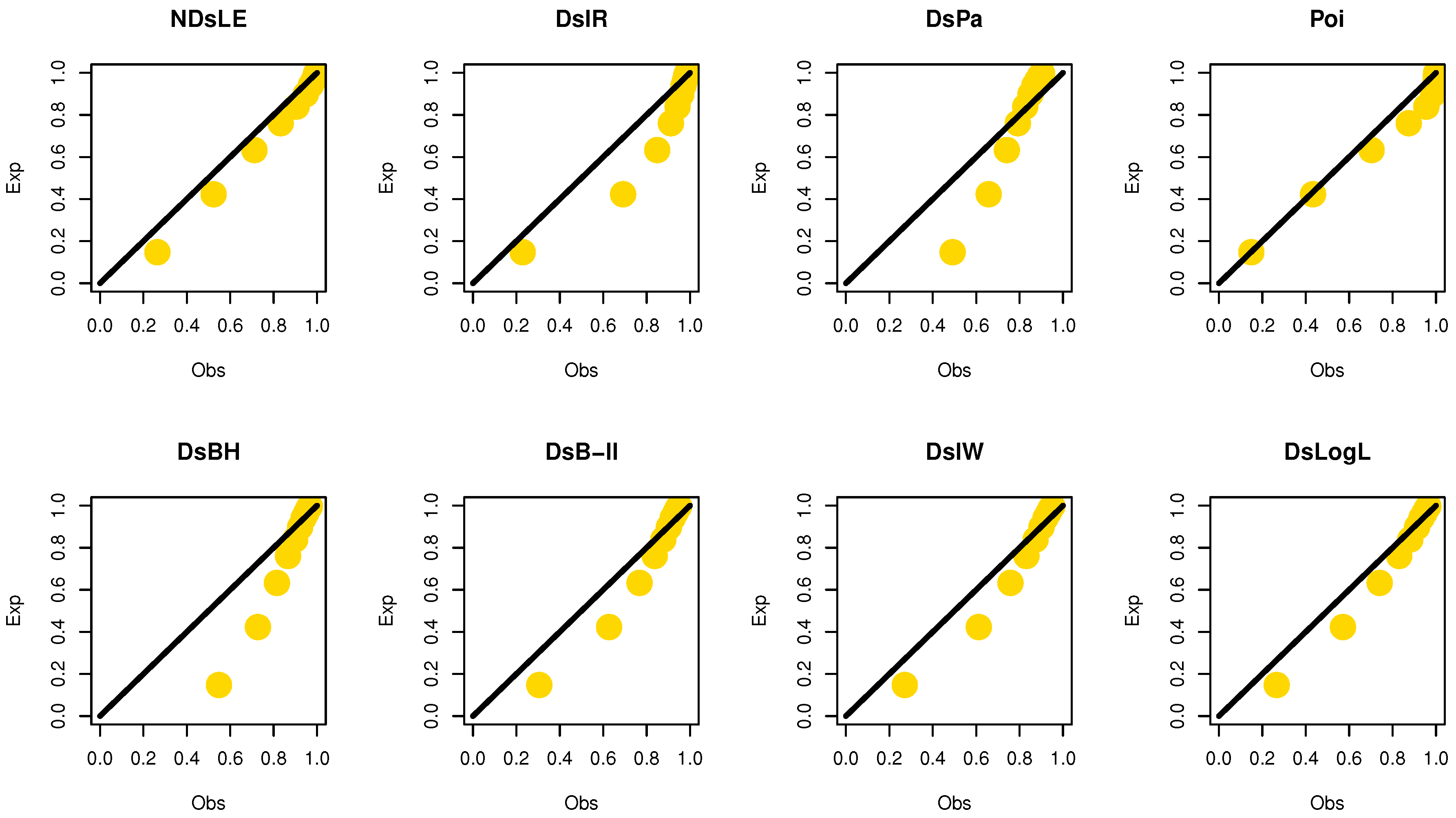
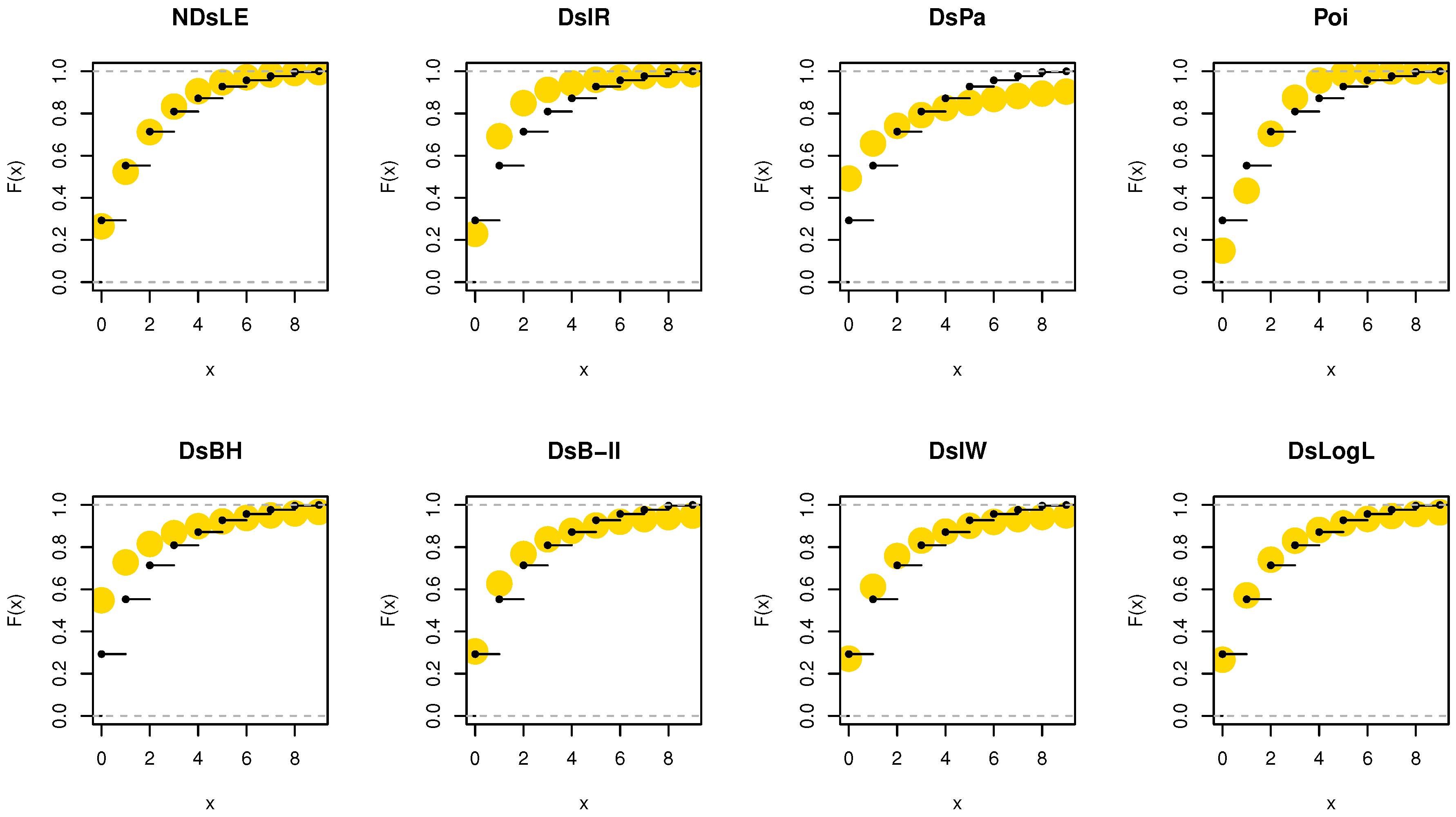
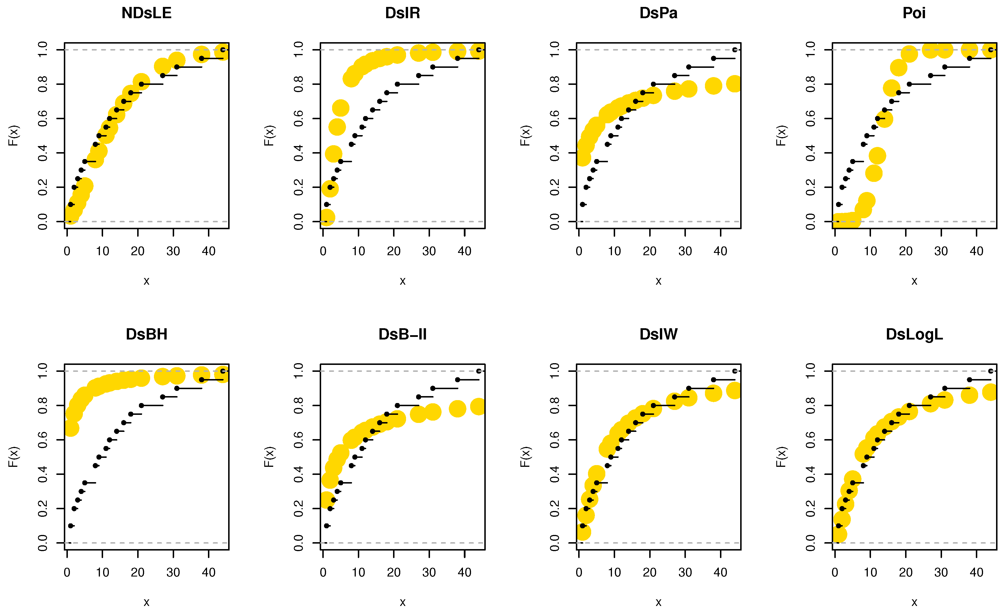
From Table 6, the NDsLE model provides the best fit among all CMs because it has the smallest value among , A, CA, B, H, and as well as the highest PV. The empirical PMF, PP, and CDF plots for data set I are displayed in Figure 7, Figure 8, and Figure 9, respectively, which indicates that the data set I plausibly came from the NDsLE model.
Table 7 lists different estimators for data set I, and it was found that the MLE and MoE techniques worked quite well for modeling data set I.
Table 8 lists some numerical accounts of empirical and theoretical descriptive statistics. It is noted that all scales were approximately equal.
6.2. Data Set II
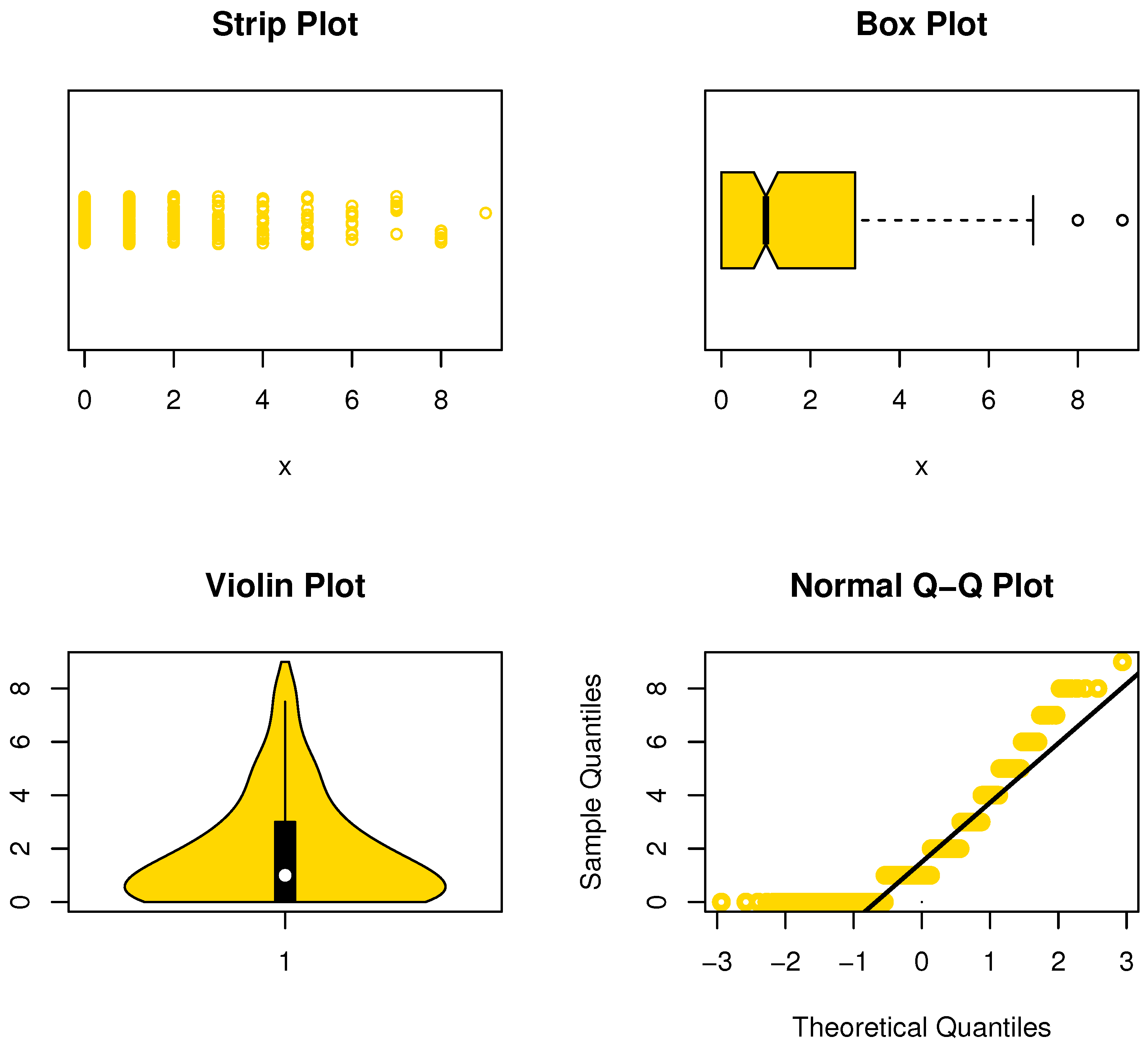
This data set was given by Karlis and Xekalaki ([21]) and represents the numbers of fires in Greece for the period from 1 July 1998 to 31 August 1998. The strip, box, violin, and QQ plots are displayed in Figure 10, and we can see that data set II is asymmetric and has some outlier observations. Table 9 introduces the MLEs with its Std-er, and C.I for the model parameter and other CMs. Moreover, the GOF measures are shown in the same Table.
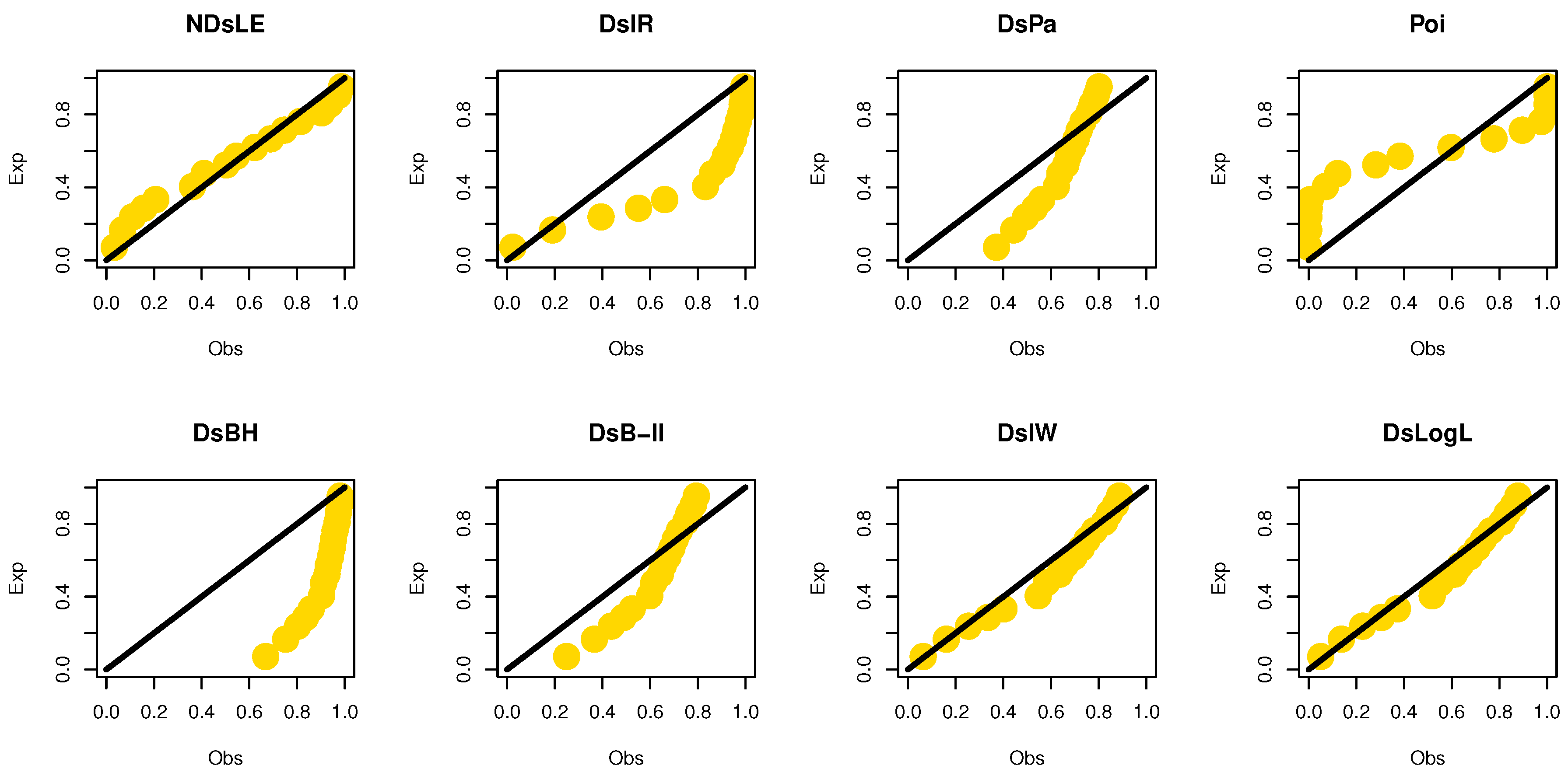
From Table 6, the NDsLE model provided the best fit among all CMs. The empirical PP and CDF plots for data set II are displayed in Figure 11 and Figure 12, respectively.
Table 10 reports various estimators for data set II, and it was found that the MLE, MoE, LSE, WLSE, and CVME methods worked quite well for modeling data set II, but the MoE approach was the best.
Table 11 reports some numerical accounts of empirical and theoretical descriptive statistics. It was found that all scales were approximately equal except that of the ProE approach.
6.3. Data Set III
The data were reported in https://www.worldometers.info/coronavirus/country/south-korea/ (accessed on 14 February 2022) and represent the daily new deaths in South Korea for COVID-19 from 15 February to 12 December 2020. In Figure 13, we can see the data are asymmetric, and some extreme observations are present. Table 12 lists the MLEs with its Std-er, GOF, and C.I for the NDsLE parameter and other CMs.
From Table 12, the NDsLE model provides the best fit among all CMs. The empirical PMF, PP, and CDF plots for data set III are displayed in Figure 14, Figure 15, and Figure 16, respectively.
Table 13 lists various estimators for data set III; it was found that the MLE and MoE techniques worked quite well for modeling data set III, but the MLE method was the best.
Table 14 listed some numerical accounts of empirical and theoretical descriptive statistics. It is clear that all scales were approximately equal.
6.4. Data Set IV
The data set represents the leukemia remission times (in weeks) for 20 patients (see Damien and Walker, [22]). The data are asymmetric-shaped and contain some extreme values (see Figure 17).
Table 15 introduces the MLEs with its Std-er, GOF, and C.I for the NDsLE parameter and other CMs.
From Table 15, the NDsLE model provided the best fit among all tested models. The empirical PPs and CDFs plots for data set IV are displayed in Figure 18 and Figure 19, respectively.
Table 16 lists different estimators for data set IV; it was found that the MLE, MoE, ProE, LSE, WLSE and CVME methods worked quite well for modeling data set IV, but the MLE approach was the best.
Table 17 report some numerical accounts of empirical and theoretical descriptive statistics. It is noted that all scales are approximately equal.
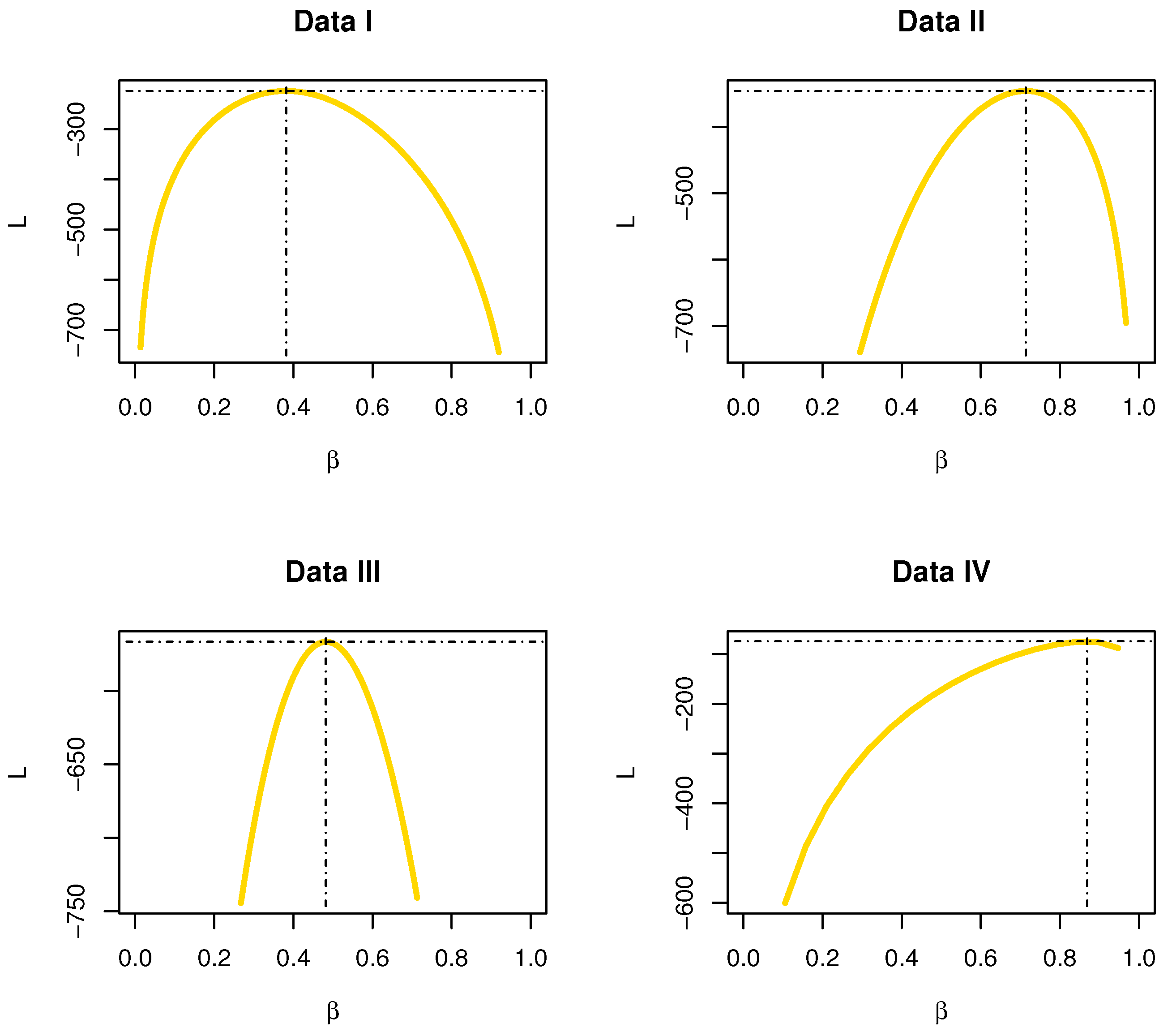
The profiles of L functions for data sets I, II, III and IV are displayed in Figure 20; it was found that the estimator was a unique “unimodal function”.
7. Conclusions
In this paper, a novel discrete model with one parameter called the discrete linear-exponential (NDsLE) model, was introduced. Its various statistical features were derived in detail. It was found that the NDsLE model was a proper model for right-skewed data sets, especially those having extreme observations. Moreover, the NDsLE model provided a wide variation in the shape of the kurtosis, and consequently it could be utilized for modeling different kinds of data. The NDsLE parameter was estimated using different estimation techniques, namely, MLE, MoE, ProE, LSE, WLSE, and CVME. Simulation studies were performed based on different sample sizes, and it was found that the six methods worked quite effectively in estimating the NDsLE parameter. Four data sets were analyzed to illustrate and prove the notability of the NDsLE model. Finally, the NDsLE model would be a better alternative to other lifetime models available in the existing literature, especially, in extreme values fields.
Funding
The author extends their appreciation to the Deputyship for Research & Innovation, Ministry of Education in Saudi Arabia for funding this research work through the project number IF-PSAU-2021/01/18291.
Data Availability Statement
The four data sets are available in the paper.
Conflicts of Interest
The author declares no conflict of interest.
References
- Roy, D. Discrete Rayleigh distribution. IEEE Trans. Reliab. 2004, 53, 255–260. [Google Scholar] [CrossRef]
- Krishna, H.; Pundir, P.S. Discrete Burr and discrete Pareto distributions. Stat. Methodol. 2009, 6, 177–188. [Google Scholar] [CrossRef]
- Eliwa, M.S.; El-Morshedy, M.; Yousof, H.M. A discrete exponential generalized-G family of distributions: Properties, with Bayesian and Non-Bayesian estimators to model medical, engineering, and agriculture data. Mathematics 2022, 10, 3348. [Google Scholar] [CrossRef]
- Gómez-Déniz, E.; Calderín-Ojeda, E. The discrete Lindley distribution: Properties and applications. J. Stat. Comput. Simul. 2011, 81, 1405–1416. [Google Scholar] [CrossRef]
- Nekoukhou, V.; Alamatsaz, M.H.; Bidram, H. Discrete generalized exponential distribution of a second type. Statistics 2013, 47, 876–887. [Google Scholar] [CrossRef]
- Nekoukhou, V.; Bidram, H. The exponentiated discrete Weibull distribution. Sort 2015, 39, 127–146. [Google Scholar]
- Hussain, T.; Aslam, M.; Ahmad, M. A two-parameter discrete Lindley distribution. Rev. Colomb. Estad. 2016, 39, 45–61. [Google Scholar] [CrossRef]
- Para, B.A.; Jan, T.R. On discrete three-parameter Burr type XII and discrete Lomax distributions and their applications to model count data from medical science. Biom. Biostat. J. 2016, 4, 1–15. [Google Scholar]
- Eliwa, M.S.; Alhussain, Z.A.; El-Morshedy, M. Discrete Gompertz-G family of distributions for over-and under-dispersed data with properties, estimation, and applications. Mathematics 2020, 8, 358. [Google Scholar] [CrossRef] [Green Version]
- El-Morshedy, M.; Eliwa, M.S.; Nagy, H. A new two-parameter exponentiated discrete Lindley distribution: Properties, estimation and applications. J. Appl. Stat. 2020, 47, 354–375. [Google Scholar] [CrossRef] [PubMed]
- Yousof, H.M.; Chesneau, C.; Hamedani, G.G.; Ibrahim, M. A new discrete distribution: Properties, characterizations, modeling real count data, Bayesian and non-Bayesian estimations. Statistica 2021. forthcoming. [Google Scholar]
- Ibrahim, M.; Ali, M.M.; Yousof, H.M. The discrete analogue of the Weibull G family: Properties, different applications, Bayesian and non-Bayesian estimation methods. Ann. Data Sci. 2021, 1–38. [Google Scholar] [CrossRef]
- Al-Bossly, A.; Eliwa, M.S. Asymmetric probability mass function for count data based on the binomial technique: Synthesis and analysis with inference. Symmetry 2022, 14, 826. [Google Scholar] [CrossRef]
- Sah, B.K. One-parameter linear-exponential distribution. Maths 2021, 6, 6–15. [Google Scholar] [CrossRef]
- Hussain, T.; Ahmad, M. Discrete inverse Rayleigh distribution. Pak. J. Stat. 2014, 30, 203–222. [Google Scholar]
- Poisson, S.D. Probabilité des Jugements en Matière Criminelle et en Matière Civile, Précédées Des règles Générales du Calcul des Probabilitiés; Bachelier: Paris, France, 1837; Volume 1, p. 1837. [Google Scholar]
- El-Morshedy, M.; Eliwa, M.S.; Altun, E. Discrete Burr-Hatke distribution with properties, estimation methods and regression model. IEEE Access 2020, 8, 74359–74370. [Google Scholar] [CrossRef]
- Jazi, M.A.; Lai, C.D.; Alamatsaz, M.H. A discrete inverse Weibull distribution and estimation of its parameters. Stat. Methodol. 2010, 7, 121–132. [Google Scholar] [CrossRef]
- Para, B.A.; Jan, T.R. Discrete version of log-logistic distribution and its applications in genetics. Int. Mod. Math. Sci. 2016, 14, 407–422. [Google Scholar]
- Chakraborty, S.; Chakravarty, D. Discrete gamma distributions: Properties and parameter estimations. Commun. Stat. Theory Methods 2012, 41, 3301–3324. [Google Scholar] [CrossRef]
- Karlis, D.; Xekalaki, E.; Lipitakis, E.A. On some discrete valued time series models based on mixtures and thinning. In Proceedings of the Fifth Hellenic-European Conference on Computer Mathematics and Its Applications, Athens, Greece, 20–22 September 2001; pp. 872–877. [Google Scholar]
- Damien, P.; Walker, S. A Bayesian non-parametric comparison of two treatments. Scand. J. Stat. 2002, 29, 51–56. [Google Scholar] [CrossRef]
Figure 1.
The PMF, HRF and RHRF plots of the NDsLE model.

Figure 2.
Some DS plots for the NDsLE model.

Figure 3.
Simulation results for under various estimation techniques.

Figure 4.
Simulation results for under various estimation techniques.

Figure 5.
Simulation results for under various estimation techniques.

Figure 6.
Nonparametric plots for data set I.

Figure 7.
The empirical PMFs plots for data set I.

Figure 8.
The empirical PPs plots for data set I.

Figure 9.
The empirical CDFs plots for data set I.

Figure 10.
Nonparametric plots for data set II.

Figure 11.
The empirical PPs plots for data set II.

Figure 12.
The empirical CDFs plots for data set II.

Figure 13.
Nonparametric plots for data set III.

Figure 14.
The empirical PMFs plots for data set III.

Figure 15.
The empirical PPs plots for data set III.

Figure 16.
The empirical CDFs plots for data set III.

Figure 17.
Nonparametric plots for data set IV.

Figure 18.
The empirical PPs plots for data set IV.

Figure 19.
The empirical CDFs plots for data set IV.

Figure 20.
The profiles of L functions for data sets I, II, III and IV.


Table 1.
Some DS for the NDsLE model under various values of .
Table 2.
The performance of different estimators.
| p | Criteria | MLE | MoE | ProE | LSE | WLSE | CVME |
|---|---|---|---|---|---|---|---|
| 20 | 0.13725150 | 0.13901581 | 0.14074285 | ||||
| NDS | |||||||
| NES | |||||||
| 50 | |||||||
| NDS | |||||||
| NES | |||||||
| 150 | |||||||
| NDS | |||||||
| NES | |||||||
| 300 | |||||||
| NDS | |||||||
| NES | |||||||
| 500 | |||||||
| NDS | |||||||
| NES | |||||||
| 700 | |||||||
| NDS | |||||||
| NES | |||||||
Table 3.
The performance of different estimators.
| p | Criteria | MLE | MoE | ProE | LSE | WLSE | CVME |
|---|---|---|---|---|---|---|---|
| 20 | 0.16739517 | ||||||
| NDS | |||||||
| NES | |||||||
| 50 | |||||||
| NDS | |||||||
| NES | |||||||
| 150 | |||||||
| NDS | |||||||
| NES | |||||||
| 300 | |||||||
| NDS | |||||||
| NES | |||||||
| 500 | |||||||
| NDS | |||||||
| NES | |||||||
| 700 | |||||||
| NDS | |||||||
| NES | |||||||
Table 4.
The performance of different estimators.
| p | Criteria | MLE | MoE | ProE | LSE | WLSE | CVME |
|---|---|---|---|---|---|---|---|
| 20 | 0.55453838 | ||||||
| NDS | |||||||
| NES | |||||||
| 50 | |||||||
| NDS | |||||||
| NES | |||||||
| 150 | |||||||
| NDS | |||||||
| NES | |||||||
| 300 | |||||||
| NDS | |||||||
| NES | |||||||
| 500 | |||||||
| NDS | |||||||
| NES | |||||||
| 700 | |||||||
| NDS | |||||||
| NES | |||||||
Table 5.
The CMs of the NDsLE model.
| Distribution | Abbreviation | Author(s) |
|---|---|---|
| Discrete inverse Rayleigh | DsIR | Hussain and Ahmad [15] |
| Discrete Pareto | DsPa | Krishna and Pundir [2] |
| Poisson | Poi | Poisson [16] |
| Discrete Burr-Hatke | DsBH | El-Morshedy et al. [17] |
| Discrete Burr type II | DsB-II | Para and Jan [8] |
| Discrete inverse Weibull | DsIW | Jazi et al. [18] |
| Discrete log-logistic | DsLog-L | Para and Jan [19] |
Table 6.
The MLEs, Std-er, C.I, and GOF measures for data set I.
| No. | EF | ||||||||
|---|---|---|---|---|---|---|---|---|---|
| X | OF | NDsLE | DsIR | DsPa | Poi | DsBH | DsB-II | DsIW | DsLogL |
| 70 | |||||||||
| 38 | |||||||||
| 17 | |||||||||
| 10 | |||||||||
| 9 | |||||||||
| 3 | |||||||||
| 2 | |||||||||
| 1 | |||||||||
| Total | |||||||||
| MLE for | |||||||||
| Std-er | |||||||||
| 95% C.I | |||||||||
| MLE for | − | − | − | − | − | ||||
| Std-er | − | − | − | − | − | ||||
| 95% C.I | |||||||||
| A | |||||||||
| CA | |||||||||
| B | |||||||||
| H | |||||||||
| DV | 3 | 3 | 4 | 2 | 4 | 2 | 3 | 2 | |
| PV | ≤0.001 | ≤0.001 | ≤0.001 | ||||||
Table 7.
CVE for data set I.
| No. | EF | ||||||
|---|---|---|---|---|---|---|---|
| X | OF | MLE | MoE | ProE | LSE | WLSE | CVME |
| 70 | |||||||
| 38 | |||||||
| 17 | |||||||
| 10 | |||||||
| 9 | |||||||
| 3 | |||||||
| 2 | |||||||
| 1 | |||||||
| Total | |||||||
| DF | 3 | 3 | 3 | 5 | 4 | 5 | |
| PV | <0.001 | <0.001 | <0.001 | ||||
Table 8.
Descriptive statistics for data set I.
| Data | |||||
| MLE | |||||
| MoE | |||||
| ProE | |||||
| LSE | |||||
| WLSE | |||||
| CVME |
Table 9.
The MLEs, Std-er, C.I, and GOF measures for data set II.
| NDsLE | DsIR | DsPa | Poi | DsBH | DsB-II | DsIW | DsLogL | ||
|---|---|---|---|---|---|---|---|---|---|
| MLE for | |||||||||
| Std-er | |||||||||
| 95% C.I | |||||||||
| MLE for | − | − | − | − | − | ||||
| Std-er | − | − | − | − | − | ||||
| 95% C.I | |||||||||
| A | |||||||||
| CA | |||||||||
| B | |||||||||
| H | |||||||||
| K–S | 0.089 | ||||||||
| PV | 0.281 | ≤0.001 | ≤0.0010 | ≤0.0010 | |||||
Table 10.
CVE for data set II.
| MLE | MoE | ProE | LSE | WLSE | CVME | |
|---|---|---|---|---|---|---|
| K–S | ||||||
| PV | ≤0.001 |
Table 11.
Descriptive statistics for data set II.
| Data | |||||
| MLE | |||||
| MoE | |||||
| ProE | |||||
| LSE | |||||
| WLSE | |||||
| CVME |
Table 12.
The MLEs, Std-er, C.I, and GOF measures for data set III.
| No. | EF | ||||||||
|---|---|---|---|---|---|---|---|---|---|
| X | OF | NDsLE | DsIR | DsPa | Poi | DsBH | DsB-II | DsIW | DsLogL |
| 89 | |||||||||
| 79 | |||||||||
| 49 | |||||||||
| 29 | |||||||||
| 19 | |||||||||
| 17 | |||||||||
| 9 | |||||||||
| 6 | |||||||||
| 6 | |||||||||
| 1 | |||||||||
| Total | |||||||||
| MLE for | |||||||||
| Std-er | |||||||||
| 95% C.I | |||||||||
| MLE for | − | − | − | − | − | ||||
| Std-er | − | − | − | − | − | ||||
| 95% C.I | |||||||||
| A | |||||||||
| CA | |||||||||
| B | |||||||||
| H | |||||||||
| DV | 6 | 6 | 7 | 4 | 6 | 6 | 6 | 6 | |
| PV | ≤0.001 | ≤0.001 | ≤0.001 | ≤0.001 | ≤0.001 | ≤0.001 | ≤0.001 | ||
Table 13.
CVE for data set III.
| No. | EF | ||||||
|---|---|---|---|---|---|---|---|
| X | OF | MLE | MoE | ProE | LSE | WLSE | CVME |
| 89 | |||||||
| 79 | |||||||
| 49 | |||||||
| 29 | |||||||
| 19 | |||||||
| 17 | |||||||
| 9 | |||||||
| 6 | |||||||
| 6 | |||||||
| 1 | |||||||
| Total | |||||||
| DV | 6 | 6 | 6 | 7 | 7 | 7 | |
| PV | ≤0.001 | ≤0.001 | |||||
Table 14.
Descriptive statistics for data set III.
| Data | |||||
| MLE | |||||
| MoE | |||||
| ProE | |||||
| LSE | |||||
| WLSE | |||||
| CVME |
Table 15.
The MLEs, Std-er, C.I, and GOF measures for data set IV.
| NDsLE | DsIR | DsPa | Poi | DsBH | DsB-II | DsIW | DsLogL | ||
|---|---|---|---|---|---|---|---|---|---|
| MLE for | |||||||||
| Std-er | |||||||||
| 95% C.I | |||||||||
| MLE for | − | − | − | − | − | ||||
| Std-er | − | − | − | − | − | ||||
| 95% C.I | |||||||||
| A | |||||||||
| CA | |||||||||
| B | |||||||||
| H | |||||||||
| K–S | |||||||||
| PV | <0.001 | <0.001 | |||||||
Table 16.
CVE for data set IV.
| MLE | MoE | ProE | LSE | WLSE | CVM | |
|---|---|---|---|---|---|---|
| K–S | ||||||
| PV |
Table 17.
Descriptive statistics for data set IV.
| Data | |||||
| MLE | |||||
| MoE | |||||
| ProE | |||||
| LSE | |||||
| WLSE | |||||
| CVME |
Publisher’s Note: MDPI stays neutral with regard to jurisdictional claims in published maps and institutional affiliations. |
© 2022 by the author. Licensee MDPI, Basel, Switzerland. This article is an open access article distributed under the terms and conditions of the Creative Commons Attribution (CC BY) license (https://creativecommons.org/licenses/by/4.0/).
Share and Cite
MDPI and ACS Style
El-Morshedy, M. A Discrete Linear-Exponential Model: Synthesis and Analysis with Inference to Model Extreme Count Data. Axioms 2022, 11, 531. https://doi.org/10.3390/axioms11100531
AMA Style
El-Morshedy M. A Discrete Linear-Exponential Model: Synthesis and Analysis with Inference to Model Extreme Count Data. Axioms. 2022; 11(10):531. https://doi.org/10.3390/axioms11100531
Chicago/Turabian StyleEl-Morshedy, Mahmoud. 2022. "A Discrete Linear-Exponential Model: Synthesis and Analysis with Inference to Model Extreme Count Data" Axioms 11, no. 10: 531. https://doi.org/10.3390/axioms11100531
Note that from the first issue of 2016, this journal uses article numbers instead of page numbers. See further details here.