

Homothetic Symmetries of Static Cylindrically Symmetric Spacetimes—A Rif Tree Approach


1
Department of Mathematics, University of Peshawar, Peshawar 25000, Khyber Pakhtunkhwa, Pakistan
2
Department of Mathematics and Sciences, Prince Sultan University, Riyadh 11586, Saudi Arabia
*
Author to whom correspondence should be addressed.
Axioms 2022, 11(10), 506; https://doi.org/10.3390/axioms11100506
Submission received: 22 August 2022
/
Revised: 21 September 2022
/
Accepted: 23 September 2022
/
Published: 26 September 2022
(This article belongs to the Section Mathematical Physics)
Abstract
:In this paper, we find all static, cylindrically symmetric spacetime metrics admitting homothetic symmetries. For this purpose, first we analyze the homothetic symmetry equations by an algorithm developed in Maple which gives all possible static, cylindrically symmetric metrics that may possess proper homothetic symmetry. After that, we have solved the homothetic symmetry equations for all these metrics to get the final form of homothetic symmetry vector fields. Comparing the obtained results with those of direct integration technique, it is observed that the Rif tree approach not only recovers the metrics already found by direct integration technique, but it also produces some new metrics.
MSC:
83C151. Introduction
The theory of general relativity was presented by Albert Einstein in 1915, and until now it has been considered as a widely accepted theory among all the existing theories of gravitation. This theory gives a generalization of the special theory of relativity, which is another scientific theory presented by Einstein in 1905 giving a relationship between space and time. Moreover, general relativity refines Newton’s law of universal gravitation and treats gravity as a warping of spacetime rather than a force that attracts objects toward each other. The warping of spacetime, known as curvature, is because of the presence of matter in the spacetime. The curvature of a spacetime is given by a tensor quantity, called an Einstein tensor, and it is denoted by In terms of metric tensor Ricci tensor , and the Ricci scalar the Einstein tensor can be expressed as The distribution of matter and energy in a spacetime is given by energy-momentum tensor , and it is related to the Einstein tensor via a system of non-linear partial differential equations, known as Einstein’s field equations (EFEs) [1],
where is a constant with G as a Newtonian constant of gravitation and c as the speed of light. The apparent look of EFEs is simple, but finding their exact solutions is much more difficult because of their nonlinear nature. However, many exact solutions of these equations have been found in the literature, and have played a pivotal role in the discussion of physical problems. Some of the known solutions of EFEs include Schwarzchild, Kerr, Reissner and Nordstrm, de Sitter, Tolman, Friedmann–Robertson–Walker, and plane wave solutions. Out of these solutions, Schwarzchild and Kerr solutions are found to be very helpful in the study of black holes. Similarly, Friedmann solutions play a key role in the field of cosmology and the plane wave solutions in discovering the existence of gravitational radiations [1]. All these exact solutions of EFEs are obtained under some assumptions, the most common being the symmetry restrictions on the metric of spacetime. Such restrictions not only help in finding the exact solution of EFEs, they are also used in the classification of the existing solutions. Killing symmetry, also called the Killing vector field (KVF), is considered to be the most basic spacetime symmetry and is defined in terms of a smooth vector field V such that the Lie derivative of the metric tensor along V turns out to be zero; that is, [2]. In order to explore KVFs for any spacetime, one requires to derive a set of Killing equations by using the relation and to solve these equations to get the explicit form of KVFs. These vector fields have been studied for some physically important spacetimes such as static, cylindrically symmetric [3], static, spherically symmetric [4] and plane symmetric spacetimes [5].
Corresponding to the KVFs admitted by a spacetime, there exist conservation laws [6]. In the literature, it is observed that most of the conservation laws in a spacetime are given by the KVFs they admit. However, there are certain conservation laws which are not given by KVFs. For example, in the Friedmann metric, there is no timelike KVF giving conservation of energy, but the same conservation law can be achieved in this metric with the help of conformal symmetries [7]. Like Killing symmetry, conformal symmetry is also defined in terms of a smooth vector field V satisfying the relation [2]
where denotes a real valued function on the spacetime. In explicit form, Equation (2) gets the form
Varying , and c from 0 to 3 in the above equation and using the Einstein’s summation convention over the repeated indices, we get a system of ten equations. The solution of these ten equations leads to the explicit form of the vector field In cases where in Equation (2) is a constant, the conformal vector field becomes a homothetic vector field (HVF). Conformal symmetries, also called conformal vector fields (CVFs) have many applications. These symmetries are used in literature as a mathematical tool for the integration of EFEs [8]. Moreover, these symmetries have interesting applications in cosmology and astrophysics [9,10]. Due to these applications, conformal symmetry attracted researchers and different spacetimes were classified via this symmetry [11,12,13,14].
The method of direct integration was used for finding all the above-defined symmetries in the aforementioned references, which is a cumbersome and time-consuming approach that also runs the risk of losing some important metrics. In order to overcome these problems and to ensure that no important spacetime metric is lost during the classification, the recent literature of general relativity uses some computer algorithms for determining all possible metrics possessing the desired symmetry. These metrics are then used to solve the symmetry equations under consideration. This approach of investigating spacetime symmetries is known as the Rif tree approach, and it has been recently used to classify some spacetime metrics according to different symmetries [15,16,17], where it has been observed that this new approach not only recovers all the metrics obtained by direct integration technique but also gives some new metrics. In this paper, we use this approach to study homothetic symmetries of the most general static, cylindrically symmetric metric.
2. Homothetic Symmetry Equations
The metric of static, cylindrically symmetric spacetimes is given by [1]
where and This metric admits at least three KVFs, given by and Out of the three metric coefficients , and if any two are same, the above metric reduces to the metric of static plane symmetric spacetimes, admitting the same three KVFs along with an additional rotational symmetry. The homothetic symmetries of static plane symmetric spacetimes were explored by using the Rif tree approach in Ref. [18]. Thus, throughout this paper we only consider static, cylindrically symmetric metrics with By using and from the above metric in Equation (2) with const., we obtain the following set of homothetic symmetry equations:
The solution of the above system leads to the explicit form of HVFs for whereas for it gives KVFs. These equations were solved in Ref. [18] by considering and using the direct integration approach. The authors obtained only two static, cylindrically symmetric metrics (other than plane symmetric) possessing proper HVFs.
In the direct integration technique, one needs to decouple the set of symmetry equations and then integrate it. Moreover, some conditions on the metric functions are also needed to solve this system. The main drawback of this approach of solving symmetry equations is that it does not provide a complete classification of the spacetime under consideration because there is no criteria for choosing the values of metric functions. On the other hand, a newly developed Rif tree approach provides a systematic way to solve the set of symmetry equations and provides many more metrics than those given by the direct integration technique. In this way, one gets a complete classification of the spacetime under consideration.
The Rif tree approach is based on a Maple algorithm, known as Rif algorithm, whose idea was first given by Reid et al. [19]. This algorithm was developed for the purpose of reduction of nonlinear systems of differential equations to reduced involutive form by using some algebraic and differentiation operations. As a result, the simplified involutive form of the system satisfies the constant-rank condition, and it contains all the integrability conditions. To start the procedure, one needs to consider a system of differential equations along with a matrix representing the ranking of the derivatives used in the equations. In the second step, the basic operations of algebra and derivatives are utilized for transforming the system to a specific form that includes all integrability conditions. The Rif algorithm is a powerful tool that can be used for reducing the complexity of the system. It also gives information about the number of solutions of a system before solving it. Though this calculation is simple, it is quite lengthy. However, one may use the “rifsimp” command with the “Exterior” package in Maple for all these calculations. The Maple command “caseplot” is used to view the output of the Rif algorithm graphically. The resulting plot is always in the form of a tree, known as Rif tree or classification tree. While solving the symmetry equations by this method, each branch of the Rif tree gives a unique metric. After that, one needs to solve the symmetry equations for all these metrics. Here, we use the Rif tree approach to solve the set of symmetry equations and prove that this approach produces many new metrics which were not listed in Ref. [18].
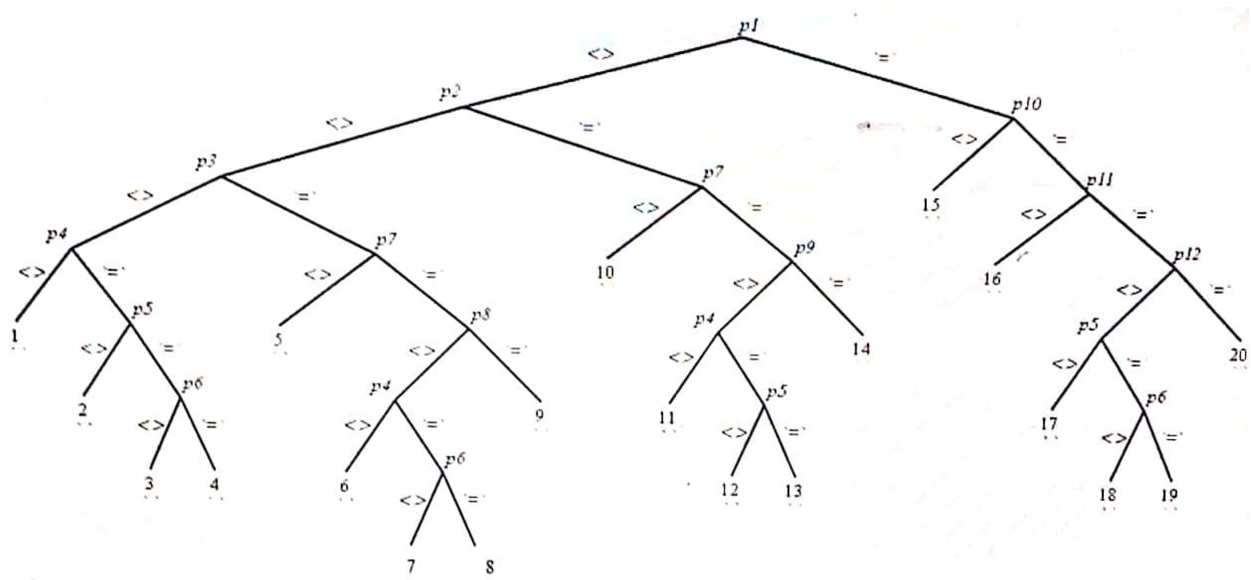
In order to find all possible static cylindrically symmetric metrics admitting HVFs, we analyze Equations (5)–(14) through the Rif algorithm. The algorithm imposes some conditions on , and C, which we then use to solve Equations (5)–(14) to get the explicit form of HVFs. These conditions are displayed in the form of branches of the Rif tree, given in Figure 1. The nodes of the Rif tree, denoted by are called pivots and are given in (15). Moreover, the symbols and “ in the tree signify whether the corresponding is zero or non-zero, respectively. In this way, every branch restricts the metric functions , and C to satisfy some conditions which are then used to solve Equations (5)–(14).
For the conditions of some branches, the solution of Equations (5)–(14) gives the minimum three KVFs with no proper homothety. Such branches are labeled by 7, 12, 17, and 18 in the Rif tree. In the remaining branches, we have either obtained one proper HVF along with three minimum KVFs or four or seven KVFs with no proper HVF. We summarize our results in the forthcoming sections.
2.1. Four HVFs
For branches 1, 5, 6, 10, 15, and the solution of Equations (5)–(14) yields four-dimensional homothetic algebra, with one proper homothety and three minimum KVFs. Moreover, some of these branches produce more than one metric, each possessing the same number of HVFs. All these metrics along with the explicit form of homothetic vector field V and the proper homothety are listed in Table 1.
Comparing our results with those of Ref. [18], one can easily observe that here we have obtained 12 static, cylindrically symmetric metrics possessing four HVFs, whereas in Ref. [18] the authors obtained only two metrics whose homothetic algebra is four-dimensional. The remaining metrics given in Ref. [18] are static plane symmetric metrics. This proves the significance of the Rif tree approach, in that it gives a complete classification of spacetime under consideration with respect to homothetic symmetries.
All the obtained metrics of this section have a non-zero Weyl tensor of Petrov type I. To check whether the obtained spacetime metrics are regular or they contain some singularity, we find the corresponding Kretschmann scalar for all these metrics. The Kretschmann scalar, denoted by is a quadratic scalar invariant defined by where is the Riemann curvature tensor and Einstein’s summation convention is applied on the repeated indices , and The Kretschmann scalar for the metric is obtained as
As the metric functions , and C are non-zero, thus Therefore, the Kretschmann scalar is finite and hence the spacetime has no singularity. In addition, because the values of K is always non-zero.
For the metric 4b, the Kretschmann scalar becomes
which is again finite, as ; otherwise, the metric functions vanish. Hence the metric 4b is regular. The structure of the Kretschmann scalar for the metrics and is the same as that of the metric with only the difference of constants involved in the values of , and Hence, the metrics and have no singularity.
Similarly, the value of K for the metric is found to be
Like the previous cases, here K is finite as Thus the metric is regular. Similarly, the Kretschmann scalar for the metrics and being similar in structure to that of the metric is finite, and hence these two metrics are also regular.
The Kretschmann scalar for the metrics , and have a similar structure with only the difference of parameters involved in the values of , and Out of these metrics, the value of K for metric is given by
which is finite because and Hence, the metrics , and have no singularity.
2.2. Four KVFs
This section contains the results of those branches of the Rif tree for which the solution of Equations (5)–(14) leads to one additional KVF, along with the three minimum ones, and no proper homothety. Such branches are labeled by 4, 8, 13, and 19 in the Rif tree. The exact form of the metrics of these branches, the components of the Killing vector field V and additional KVFs are given in Table 2.
A complete classification of the static cylindrically symmetric spacetimes via their KVFs was presented in Ref. [3], where the authors solved the set of Killing equations by direct integration approach. However, like the case of homotheties, the metrics obtained here by Rif tree approach were not listed in Ref. [3].
The Weyl tensor for all the metrics of this section vanishes; therefore, all these metrics are conformally flat and are of Petrov type O. The Kretschmann scalar for the metric is obtained as
which is always finite. Thus, the metric is regular. The structure of Kretschmann scalar for the remaining three metrics is similar, with only the difference of parameters involved in the metric functions. For metric it has the value
which is clearly finite. Hence, all three metrics given by and are regular.
2.3. Seven KVFs
The branches 9, 14, and 20 of the Rif tree produce metrics admitting seven KVFs, out of which three are the minimum ones and the extra four KVFs along with the components of vector field V, are given in Table 3, Table 4 and Table 5. Like the previous section, these three metrics were not found in Ref. [3].
For all the three metrics of this section, the Weyl tensor vanishes; thus, all these metrics are conformally flat and of Petrov type O. The Kretschmann scalar for all these three metrics is given by showing that these metrics have no singularity.
3. Conclusions
In this paper, we have explored HVFs of static, cylindrically symmetric spacetimes. Instead of the frequently used method of directly integrating the homothetic symmetry equations, we have analyzed these equations by using the Rif algorithm that gives many static, cylindrically symmetric metrics possessing different dimensional homothetic and Killing algebras. Out of these, twelve metrics admit one proper HVF along with three minimum KVFs of the spacetimes under consideration. The remaining metrics possess three, four, or seven KVFs with no proper homothety. By finding the Lie algebra of the obtained vector fields by using the relation one can easily check that the structure of Lie algebra for each metric is different from that of all other metrics. Thus, no two of these metrics are connected by coordinate transformations. We have also calculated the Weyl tensor for all the obtained metrics, and it is observed that for the metrics admitting proper HVFs, the Weyl tensor is Petrov type I. For the metrics of Section 2.3, the Weyl tensor vanishes, and therefore these are Petrov type O metrics. By finding the Kretschmann scalar, it is conjectured that all the obtained metrics during our classification are regular.
Comparing our result with those obtained in an earlier study by direct integration technique, it is observed that the Rif tree approach recovers all the metrics given by direct integration method, and it also produces many extra metrics. Thus, the Rif tree approach is a better choice to be used for the classification of spacetimes via their Killing and homothetic symmetries.
Author Contributions
Investigation, J.K.; Supervision, T.H.; Methodology, D.S., Software, N.M. All authors have read and agreed to the published version of the manuscript.
Funding
Prince Sultan University, Riyadh, Saudi Arabia.
Data Availability Statement
Not applicable.
Acknowledgments
The authors D. Santina and N. Mlaiki would like to thank Prince Sultan University for paying the publication fee for this work through TAS LAB. All the authors are thankful to the referees for their invaluable suggestions for the improvement of the manuscript.
Conflicts of Interest
The authors declare no conflict of interest.
References
- Stephani, H.; Kramer, D.; Maccallum, M.; Hoenselaers, C.; Herlt, E. Exact Solutions of Einsteins Field Equations, 2nd ed.; Cambridge University Press: Cambridge, UK, 2003. [Google Scholar]
- Hall, G.S. Symmetries and Curvature Structure in General Relativity; World Scientific: London, UK, 2004. [Google Scholar]
- Qadir, A.; Ziad, M. Classification of Static Cylindrically Symmetric Space-Times. Il. Nuov. Cim. B 1995, 110, 277–290. [Google Scholar] [CrossRef]
- Bokhari, A.H.; Qadir, A. Symmetries of Static Spherically Symmetric Space-Times. J. Math. Phys. 1987, 28, 1019–1022. [Google Scholar] [CrossRef]
- Feroze, T.; Qadir, A.; Zaid, M. The Classification of Plane Symmetric Spacetimes by Isometries. J. Math. Phys. 2001, 42, 4947–4955. [Google Scholar] [CrossRef]
- Bokhari, A.H.; Karim, M.; Al-Sheikh, D.N.; Zaman, F.D. Circularly Symmetric Static Metric in Three Dimensions and its Killing Symmetry. Int. J. Theor. Phys. 2008, 47, 2672–2678. [Google Scholar] [CrossRef]
- Khan, S.; Hussain, T.; Bokhari, A.H.; Khan, G.A. Conformal Killing Vectors of Plane Symmetric Four Dimensional Lorentzian Manifolds. Eur. Phys. J. C 2015, 75, 523–531. [Google Scholar] [CrossRef]
- Kramer, D.; Carot, J. Conformal Symmetry of Perfect Fluids in General Relativity. J. Math. Phys. 1991, 32, 1857–1860. [Google Scholar] [CrossRef]
- Chrobok, T.; Borzeszkowski, H.H. Thermodinamical Equilibrium and Spacetime Geometry. Gen. Rel. Grav. 2006, 38, 397–415. [Google Scholar] [CrossRef]
- Mak, M.K.; Harko, T. Quark Stars Admitting a One-parameter Group of Conformal Motions. Int. J. Mod. Phys. D 2004, 13, 149–156. [Google Scholar] [CrossRef]
- Moopanar, S.; Maharaj, S.D. Conformal Symmetries of Spherical Spacetimes. Int. J. Theor. Phys. 2010, 49, 1878–1885. [Google Scholar] [CrossRef]
- Maartens, R.; Maharaj, S.D.; Tupper, B.O.J. General Solution and Classification of Conformal Motions in Static Spherical Spacetimes. Class. Quant. Grav. 1995, 12, 2577–2586. [Google Scholar] [CrossRef]
- Hall, G.S.; Carot, J. Conformal Symmetries in Null Einstein-Maxwell Fields. Class. Quant. Grav. 1994, 11, 475–480. [Google Scholar] [CrossRef]
- Maartens, R.; Maharaj, S.D. Conformal Symmetries of pp-waves. Class. Quant. Grav. 1991, 8, 503–514. [Google Scholar] [CrossRef]
- Hussain, T.; Nasib, U.; Khan, F.; Farhan, M. An Efficient Rif Algorithm for the Classification of Kantowski-Sachs Spacetimes via Conformal Vector Fields. J. Kor. Phys. Soc. 2020, 76, 286–291. [Google Scholar] [CrossRef]
- Hussain, T.; Nasib, U.; Farhan, M.; Bokhari, A.H. A study of Energy Conditions in Kantowski-Sachs Spacetimes via Homothetic Vector Fields. Int. J. Geom. Meth. Mod. Phys. 2020, 17, 1–15. [Google Scholar] [CrossRef]
- Bokhari, A.H.; Hussain, T.; Khan, J.; Nasib, U. Proper Homothetic Vector Fields of Bianchi Type I Spacetimes via Rif Tree Approach. Resul. Phys. 2021, 25, 104299. [Google Scholar] [CrossRef]
- Shabbir, G.; Ramzan, M. Classification of Cylindrically Symmetric Static Spacetimes According to Their Proper Homothetic vector Fields. Appl. Sci. 2007, 9, 148–154. [Google Scholar]
- Reid, G.J.; Wittkope, A.D.; Boulton, A. Reduction of Systems of Nonlinear Partial Differential Equations to Simplified Involutive Forms. Euro. J. Appl. Math. 1996, 7, 635–666. [Google Scholar] [CrossRef]
Figure 1.
Rif Tree.


Table 1.
Metrics admitting four HVFs.
| No. | Metric | Proper HVF | |
|---|---|---|---|
| 4a. | |||
| (Branch 1) | |||
| 4b. | |||
| (Branch 1) | |||
| 4c. | |||
| (Branch 1) | |||
| 4d. | |||
| (Branch 1) | |||
| 4e. | |||
| (Branch 5) | |||
| 4f. | |||
| (Branch 5) | |||
| 4g. | |||
| (Branch 6) | |||
| 4h. | |||
| (Branch 10) | |||
| 4i. | |||
| (Branch 10) | |||
| 4j. | |||
| (Branch 15) | |||
| 4k. | |||
| (Branch 15) | |||
| 4l. | |||
| (Branch 16) |
Table 2.
Metrics admitting four KVFs.
| No. | Metric | Vector Field Components | Additional KVFs |
|---|---|---|---|
| 4(i). | |||
| (Branch 4) | |||
| where | |||
| 4(ii). | |||
| (Branch 8) | |||
| where | |||
| 4(iii). | |||
| (Branch 13) | |||
| where | |||
| 4(iv). | |||
| (Branch 19) | |||
| where |
Table 3.
Metrics admitting seven KVFs.
| No. | Metric | Vector Field Components | Additional KVFs |
|---|---|---|---|
| 7a. | |||
| (Branch 9) | |||
| , | |||
| where | |||
Table 4.
Metrics admitting seven KVFs.
| No. | Metric | Vector Field Components | Additional KVFs |
|---|---|---|---|
| 7b. | |||
| (Branch 14) | |||
| , | |||
| where | |||
Table 5.
Metrics admitting seven KVFs.
| No. | Metric | Vector Field Components | Additional KVFs |
|---|---|---|---|
| 7c. | |||
| (Branch 20) | |||
| , | |||
| where | |||
Publisher’s Note: MDPI stays neutral with regard to jurisdictional claims in published maps and institutional affiliations. |
© 2022 by the authors. Licensee MDPI, Basel, Switzerland. This article is an open access article distributed under the terms and conditions of the Creative Commons Attribution (CC BY) license (https://creativecommons.org/licenses/by/4.0/).
Share and Cite
MDPI and ACS Style
Khan, J.; Hussain, T.; Santina, D.; Mlaiki, N. Homothetic Symmetries of Static Cylindrically Symmetric Spacetimes—A Rif Tree Approach. Axioms 2022, 11, 506. https://doi.org/10.3390/axioms11100506
AMA Style
Khan J, Hussain T, Santina D, Mlaiki N. Homothetic Symmetries of Static Cylindrically Symmetric Spacetimes—A Rif Tree Approach. Axioms. 2022; 11(10):506. https://doi.org/10.3390/axioms11100506
Chicago/Turabian StyleKhan, Jamshed, Tahir Hussain, Dania Santina, and Nabil Mlaiki. 2022. "Homothetic Symmetries of Static Cylindrically Symmetric Spacetimes—A Rif Tree Approach" Axioms 11, no. 10: 506. https://doi.org/10.3390/axioms11100506
Note that from the first issue of 2016, this journal uses article numbers instead of page numbers. See further details here.