A Numerical Method for a Heat Conduction Model in a Double-Pane Window

Abstract

In this article, we propose a one-dimensional heat conduction model for a double-pane window with a temperature-jump boundary condition and a thermal lagging interfacial effect condition between layers. We construct a second-order accurate finite difference scheme to solve the heat conduction problem. The designed scheme is mainly based on approximations satisfying the facts that all inner grid points has second-order temporal and spatial truncation errors, while at the boundary points and at inter-facial points has second-order temporal truncation error and first-order spatial truncation error, respectively. We prove that the finite difference scheme introduced is unconditionally stable, convergent, and has a rate of convergence two in space and time for the $L_{\infty }$-norm. Moreover, we give a numerical example to confirm our theoretical results.

1. Introduction

In the last decades, there is an increasing interest in the research and development of mathematical models related with clean technologies; see, for instance, [1]. The interest is motivated by the diminution of adverse environmental impacts of conventional energies, the growth of world population with improved life standards, the reduction in energy production costs, and the optimization of energy consumption [2]. It is known that about a third of the total energy is used in buildings and a about a third of energy is lost through windows [3]. Then, a key aspect to understand in order to save energy in buildings is the design of appropriate windows.

In the recent literature, there are several works focused in the study of heat transfer in pane windows [4,5,6,7,8,9,10,11,12,13,14]. The finite difference techniques is used to solve numerically the Boussinesq equations and to simulate the flow of the air in a window cavity [4]. The problem of natural convective flows in the cavity of a double-glazed window with photovoltaic cells is modeled and simulated by the Navier–Stokes and energy equations [5]. From a stationary two-dimensional formulation of heat transfer through a triple-pane window and applying the method of numerical modeling, we deduced that the thermal resistance of the triple-pane window filled with air turns out to be $1.7$ times higher than that of the double-pane window having the same thickness as the triple-pane [6]. The determination of the optimum thickness of the air layer that is trapped between the interior and exterior glass of a window pane has been studied in the context of window design [7,13]. The research of other potential problems arising in pane windows (such as the low consumption of energy in a building with double pane window, the numerical modeling, the design of multiple pane windows, the relation to the climate, etc.) are conducted by several works [8,9,10,11,12,14].

The study of transfer heat problems between different substances, for instance, solids of different types or solids and fluids, are considered by several researchers [15,16,17,18,19,20,21,22,23]. The motivations are of different types: simple examples, analytical solutions, creation of mathematical models, different applications, theoretical study, and numerical simulations [15]. Particularly, in relation to the numerical solutions, we propose several numerical methods including the use of high-order implicit time integration schemes [17], hybrid boundary element method and radial basis integral equation [18], high-order finite volume schemed [19], projection method [20], high-order implicit Runge–Kutta schemes [21], and finite difference methods [23].

On the other hand, we know that for situations of very-low temperatures near absolute zero the heat propagate at a finite speed [24]. Then, the classical models of heat transfer, based on the Fourier law, needs an improvement. One of those generalizations is the well-known dual-phase-lagging model proposed by Tzou in [25] (see also [26]), which is based in non-Fourier heat conduction law and the energy equation given by

$$\begin{array}{cc}\hfill q(x,t+{\tau }_q)& =-k\frac{\partial T}{\partial x}(x,t+{\tau }_T),\hfill \end{array}$$

(1)

$$\begin{array}{cc}\hfill -\frac{\partial q}{\partial x}(x,t)& =C\frac{\partial T}{\partial t}(x,t)+Q(x,t),\hfill \end{array}$$

(2)

respectively; where t is the time, x is the space position, T is the temperature, q is the heat flux, k is the heat conductivity, ${\tau }_T$ is the phase lag of the temperature gradient, ${\tau }_q$ is the phase lag of the heat flux, C is the heat capacity of the material, and Q is the volumetric heat generation. By applying a Taylor series expansion in (1), we deduce that

$$\begin{array}{c}\hfill q(x,t)+{\tau }_q\frac{\partial q}{\partial x}(x,t)=-k\left[\frac{\partial T}{\partial x}(x,t)+{\tau }_T\frac{{\partial }^{2}T}{\partial t\partial x}(x,t)\right].\end{array}$$

(3)

Then, by using (2) in (3), we obtain

$$\begin{array}{c}\hfill C\left(\frac{\partial T}{\partial t}+{\tau }_q\frac{{\partial }^{2}T}{\partial t\partial x}\right)=k\left(\frac{{\partial }^{2}T}{\partial x^2}+{\tau }_T\frac{{\partial }^{3}T}{\partial t{\partial }^{2}x}\right),\end{array}$$

(4)

which is known as the heat conduction equation under the dual-phase-lagging effect or briefly as dual-phase-lagging model.

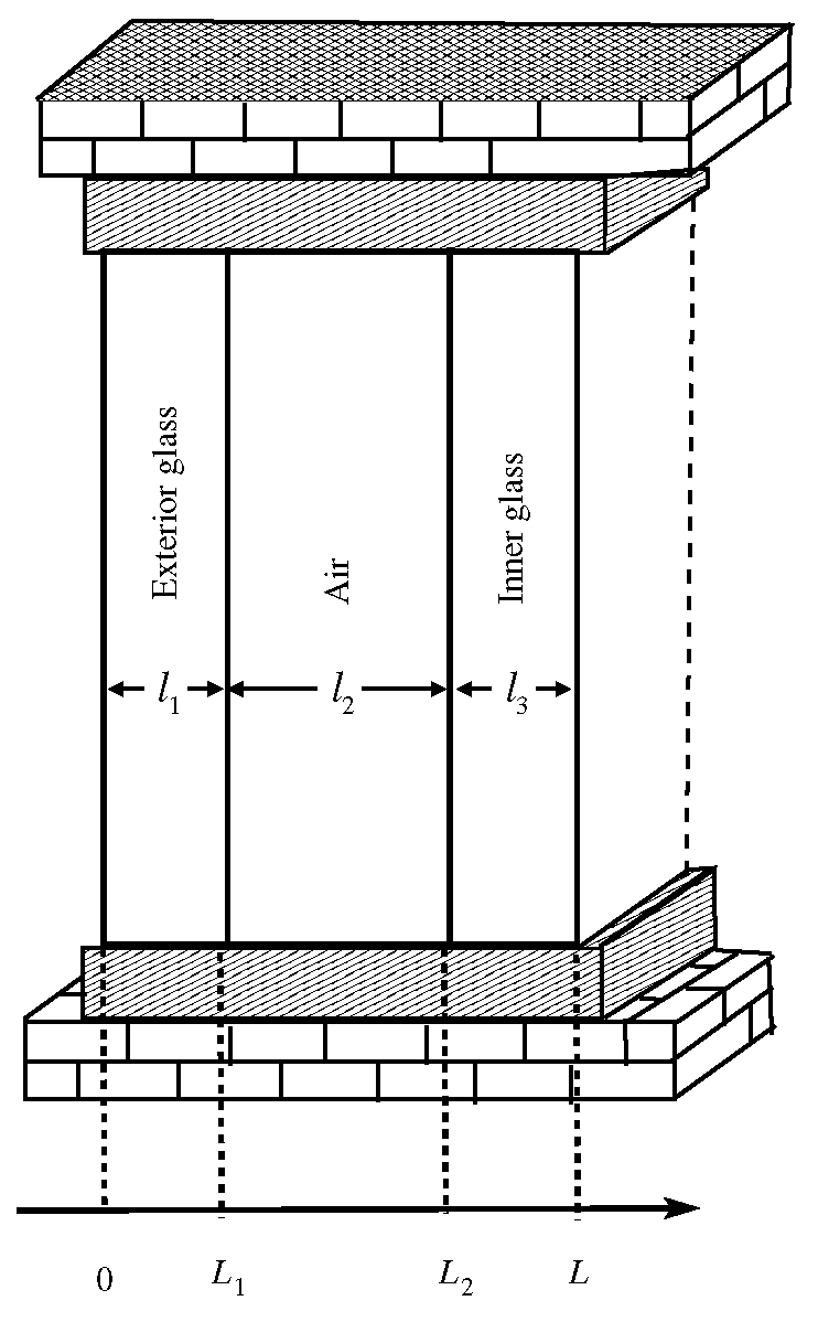
In this paper, we are interested in the problem of heat transfer in a double pane window. Let us consider a double pane window of a total width thickness L, schematically presented in Figure 1. The width thickness of exterior glass, air space, and interior glass are given by ${\ell }_1,{\ell }_2$, and ${\ell }_3$, respectively. For convenience of the presentation, we introduce the following terminology and notation

$$\begin{array}{c}\hfill \left.\begin{array}{c}{L}_0=0,L_1={\ell }_1,L_2={\ell }_1+{\ell }_2,L_3={\ell }_1+{\ell }_2+{\ell }_3=L,\hfill \\ L_0 \mathrm{and}{L}_3 \mathrm{are} \mathrm{called} \mathrm{the} \mathrm{boundaries} \mathrm{and} L_1 \mathrm{and} L_2 \mathrm{the} \mathrm{interfaces},\hfill \\ {\mathcal{I}}_1=]L_0,L_1[,{\mathcal{I}}_2=]L_1,L_2[, \mathrm{and} {\mathcal{I}}_3=]L_2,L_3[, \mathrm{are} \mathrm{called} \mathrm{the} \mathrm{layers},\hfill \\ {\mathcal{I}}^{lay}={\mathcal{I}}_1\cup {\mathcal{I}}_2\cup {\mathcal{I}}_3,{\mathcal{I}}^{int}=\left\{L_1\right\}\cup \left\{L_2\right\},\mathcal{I}={\mathcal{I}}^{lay}\cup {\mathcal{I}}^{int},\hfill \\ \partial \mathcal{I}=\{L_0,L_1\},{\mathcal{I}}_{\ell ,T}=\left\{L_{\ell }\right\}\times [0,T],Q_{\ell ,T}={\mathcal{I}}_{\ell }\times [0,T],\hfill \\ Q_T^{lay}={\mathcal{I}}^{lay}\times [0,T],I_T^{int}=I^{int}\times [0,T],Q_T=Q_T^{lay}\cup {\mathcal{I}}_T^{int}.\hfill \end{array}\right\}\end{array}$$

(5)

We assume that the mathematical model for heat transfer is given by the initial interface-boundary value problem

$$\begin{array}{cc}{C}_{\ell }\left(\frac{\partial u}{\partial t}+{\tau }_q^{(\ell )}\frac{{\partial }^{2}u}{\partial t^2}\right)=k_{\ell }\left(\frac{{\partial }^{2}u}{\partial x^2}+{\tau }_T^{(\ell )}\frac{{\partial }^{3}u}{\partial t\partial x^2}\right)+f_{\ell }(x,t),\ell =1,2,3,\hfill & \hfill \mathrm{in}{Q}_T^{lay},\end{array}$$

(6)

$$\begin{array}{cc}u(x,0)={\psi }_1\left(x\right),\frac{\partial u}{\partial t}(x,0)={\psi }_2\left(x\right),\hfill & \hfill \mathrm{on}\mathcal{I},\end{array}$$

(7)

$$\begin{array}{ccc}\left(-{\alpha }_1{K}_n^{\left(1\right)}\frac{\partial u}{\partial x}+u\right)(L_0,t)={\phi }_1\left(t\right),\hfill & \hfill & \hfill \mathrm{on}[0,T],\end{array}$$

(8)

$$\begin{array}{ccc}\left({\alpha }_2{K}_n^{\left(2\right)}\frac{\partial u}{\partial x}+u\right)(L_3,t)={\phi }_2\left(t\right),\hfill & \hfill & \hfill \mathrm{on}[0,T],\end{array}$$

(9)

$$\begin{array}{ccc}u(x-0,t)=u(x+0,t),\hfill & \hfill & \hfill \mathrm{on}{I}_T^{int},\\ k_{\ell }\left(\frac{\partial u}{\partial x}+{\tau }_T^{(\ell )}\frac{{\partial }^{2}u}{\partial x\partial t}\right)(x-0,t)\hfill & \hfill & \hfill \end{array}$$

(10)

$$\begin{array}{cccc}\hfill & =k_{\ell +1}\left(\frac{\partial u}{\partial x}+{\tau }_T^{(\ell +1)}\frac{{\partial }^{2}u}{\partial x\partial t}\right)(x+0,t),\ell =1,2,\hfill & \hfill & \mathrm{on}{I}_T^{int},\hfill \end{array}$$

(11)

where $u(x,t)$ is the temperature at the position x and time t, $C_{\ell }$ is the heat capacitance; ${\tau }_q^{(\ell )}$ and ${\tau }_T^{(\ell )}$ stand for the heat flux and the temperature gradient phase lags, respectively; $k_{\ell }$ is the conductivity; $f_{\ell }$ are the source functions; ${\alpha }_1$ and ${\alpha }_2$ are some coefficients; $K_n^{\left(1\right)}$ and $K_n^{\left(2\right)}$ are the Knudsen numbers; ${\psi }_1$ and ${\psi }_2$ are the initial conditions; and ${\phi }_1$ and ${\phi }_2$ are two given functions modeling the boundary conditions. We notice three facts: the relationship between $K_n$ and k is given by $K_n^{2}C{L}_c^2=3k{\tau }_q$ with $L_c$ a characteristic length, the boundary conditions (8) and (9) are a consequence of assuming a temperature-jump condition, and the model are not in dimensionless form; see [27,28] for details.

The state equation (Equation (6)) is deduced by assuming by the fact that the dual-phase-lagging model of the form (4) is satisfied in each layer ${\mathcal{I}}_1,{\mathcal{I}}_2$ and ${\mathcal{I}}_3$. The interfacial conditions (10) and (11) are imposed in order to obtain a continuous behavior of temperature and the heat flux, respectively. For instance at $x=L_1$, we have that (11), by application of the first-order non-Fourier’s law, is rewritten as follows

$$\begin{array}{c}\hfill q(L_1-0,t)+{\tau }_q^{\left(1\right)}\frac{\partial q}{\partial t}(L_1-0,t)=q(L_1+0,t)+{\tau }_q^{\left(2\right)}\frac{\partial q}{\partial t}(L_1+0,t).\end{array}$$

The condition of the type (11) was introduced in [27] for the case of the mathematical model of a double-layered nano-scale thin film, where the authors observe that these kind of interfacial conditions plays an important role in the derivation of energy estimations. Other important aspect of the mathematical model (6) and (11) is the fact the state equation and the boundary conditions (8) and (9) are given only in terms of the temperature, which is different from the standard models where a variable the heat flux is considered.

The main results of the paper are the following: (i) we prove an energy estimate, (ii) we introduce a second-order accurate finite difference scheme for solving the mathematical model, and (iii) we prove that the unconditional stability, the convergence, and estimate that the rate of convergence is two in space and time for the $L_{\infty }$-norm. Additionally, we give two numerical examples.

The methodology used in the paper is a generalization of the one introduced in [27] for the case heat transfer in a double-layered nano-scale thin film. We consider the change variable $v=u_t$ and deduce the equivalent system to (6)–(11) in terms of u and v. We introduce the discretization by a semidiscrete finite difference scheme. In addition, we deduce a fully finite difference scheme, approaching the system for $(u,v)$. We rewrite the discrete scheme to approximate the solution of (6)–(11). Then, we introduce and prove the results of discrete energy estimation, unconditional stability, convergence, and error estimates.

2. Change of Variable and Continuous Energy Estimation

We introduce a new function $v:\overline{Q_T}\to \mathbb{R}$ such that $v=u_t$. Then, from (6)–(11), we deduce that

$$\begin{array}{cccc}\hfill & C_{\ell }\left(v+{\tau }_q^{(\ell )}\frac{\partial v}{\partial t}\right)=k_{\ell }\frac{{\partial }^2}{\partial x^2}\left(u+{\tau }_T^{(\ell )}v\right)+f_{\ell }(x,t),\ell =1,2,3,\hfill & \hfill & \mathrm{in} Q_T^{lay},\hfill \end{array}$$

(12)

$$\begin{array}{cccc}\hfill & v(x,t)=\frac{\partial }{\partial t}u(x,t),\hfill & \hfill & \mathrm{in} Q_T,\hfill \end{array}$$

(13)

$$\begin{array}{cccc}\hfill & u(x,0)={\psi }_1\left(x\right),v(x,0)={\psi }_2\left(x\right),\hfill & \hfill & \mathrm{on} \mathcal{I},\hfill \end{array}$$

(14)

$$\begin{array}{cccc}\hfill & -{\alpha }_1{K}_n^{\left(1\right)}\frac{\partial }{\partial x}\left(u+{\tau }_T^{\left(1\right)}v\right)(L_0,t)+(u+{\tau }_T^{\left(1\right)}v)(L_0,t)={\varphi }_1\left(t\right),\hfill & \hfill & \mathrm{on} [0,T],\hfill \end{array}$$

(15)

$$\begin{array}{cccc}\hfill & {\alpha }_2{K}_n^{\left(2\right)}\frac{\partial }{\partial x}\left(u+{\tau }_T^{\left(3\right)}v\right)(L_3,t)+(u+{\tau }_T^{\left(3\right)}v)(L_3,t)={\varphi }_2\left(t\right),\hfill & \hfill & \mathrm{on} [0,T],\hfill \end{array}$$

(16)

$$\begin{array}{cccc}\hfill & u(x-0,t)=u(x+0,t),v(x-0,t)=v(x+0,t),\hfill & \hfill & \mathrm{on} I_T^{int},\hfill \end{array}$$

(17)

$$\begin{array}{cccc}\hfill & k_{\ell }\frac{\partial }{\partial x}\left(u+{\tau }_T^{(\ell )}v\right)(x-0,t)=k_{\ell +1}\frac{\partial }{\partial x}\left(u+{\tau }_T^{(\ell +1)}v\right)(x+0,t),\hfill & \hfill & \mathrm{on} I_T^{int},\hfill \end{array}$$

(18)

where ${\varphi }_i={\phi }_i+{\tau }_T^{\left(i\right)}{\left({\phi }_i\right)}_t$ for $i=1,2$.

Theorem 1.

Consider the notation and terminology defined on (5) and $u,v$ solutions of (6)–(11) and (12)–(18) with boundary conditions ${\varphi }_1={\varphi }_2=0$, respectively. If we denote by E the function defined as follows

$$\begin{array}{cc}\hfill E\left(t\right)=& \sum _{\ell =1}^3{C}_{\ell }{\tau }_q^{(\ell )}\parallel v^2{\parallel }_{L^2\left({\mathcal{I}}_{\ell }\right)}^2+\sum _{\ell =1}^3{k}_{\ell }{\parallel u_x\parallel }_{L^2\left({\mathcal{I}}_{\ell }\right)}^2+\frac{u^2(L_0,t)}{{\alpha }_1{K}_n^{\left(1\right)}}+\frac{u^2(L_3,t)}{{\alpha }_2{K}_n^{\left(2\right)}}·\hfill \end{array}$$

(19)

Then, the estimate

$$\begin{array}{c}\hfill E\left(t\right)\le E\left(0\right)+\frac{1}{2}{\int }_0^t\sum _{\ell =1}^3\frac{1}{C_{\ell }}{\int }_{{\mathcal{I}}_{\ell }}{f}_{\ell }^2(x,s)dxds,\end{array}$$

(20)

is valid for any $t\in ]0,T].$

Proof. 

Multiplying the Equation (12) by v, integrating over ${\mathcal{I}}^{lay}$, using the identities

$$\begin{array}{cc}\hfill & {\int }_{{\mathcal{I}}_{\ell }}\frac{\partial v}{\partial t}vdx=\frac{1}{2}\frac{d}{dt}{\int }_{{\mathcal{I}}_{\ell }}{v}^{2}dx,\hfill \\ \hfill & {\int }_{{\mathcal{I}}_{\ell }}\frac{\partial u}{\partial x}\frac{\partial v}{\partial x}dx=\frac{1}{2}\frac{d}{dt}{\int }_{{\mathcal{I}}_{\ell }}{\left(\frac{\partial u}{\partial x}\right)}^{2}dx,\hfill \\ \hfill & {\int }_{{\mathcal{I}}_{\ell }}\frac{{\partial }^2}{\partial x^2}\left(u+{\tau }_T^{(\ell )}v\right)vdx=\left(\frac{\partial }{\partial x}(u+{\tau }_T^{(\ell )}v)v\right)(L_{\ell }+,t)\hfill \\ \hfill & -\left(\frac{\partial }{\partial x}(u+{\tau }_T^{(\ell )}v)v\right)(L_{\ell -1}-,t)-{\int }_{{\mathcal{I}}_{\ell }}\frac{\partial u}{\partial x}\frac{\partial v}{\partial x}dx-{\tau }_T^{(\ell )}{\int }_{{\mathcal{I}}_{\ell }}{\left(\frac{\partial v}{\partial x}\right)}^{2}dx,\hfill \end{array}$$

for $\ell =1,2,3,$ and the interface conditions (17) and (18), we have that

$$\begin{array}{cc}\hfill & \sum _{\ell =1}^3{C}_{\ell }{\int }_{{\mathcal{I}}_{\ell }}{v}^{2}dx+\frac{1}{2}\sum _{\ell =1}^3{C}_{\ell }{\tau }_q^{(\ell )}\frac{d}{dt}{\int }_{{\mathcal{I}}_{\ell }}{v}^{2}dx\hfill \\ \hfill & =\sum _{\ell =1}^3{k}_{\ell }\left[\left(\frac{\partial }{\partial x}(u+{\tau }_T^{(\ell )}v)v\right)(L_{\ell }+,t)-\left(\frac{\partial }{\partial x}(u+{\tau }_T^{(\ell )}v)v\right)(L_{\ell -1}-,t)\right]\hfill \\ \hfill & -\sum _{\ell =1}^d{k}_{\ell }{\int }_{{\mathcal{I}}_{\ell }}\frac{\partial u}{\partial x}\frac{\partial v}{\partial x}dx-\sum _{\ell =1}^3{k}_{\ell }{\tau }_T^{(\ell )}{\int }_{{\mathcal{I}}_{\ell }}{\left(\frac{\partial v}{\partial x}\right)}^{2}dx+\sum _{\ell =1}^3{\int }_{{\mathcal{I}}_{\ell }}{f}_{\ell }(x,t)vdx\hfill \\ \hfill & =k_3\left(\frac{\partial }{\partial x}(u+{\tau }_T^{\left(d\right)}v)v\right)(L_d,t)-k_1\left(\frac{\partial }{\partial x}(u+{\tau }_T^{\left(1\right)}v)v\right)(L_0,t)\hfill \\ \hfill & -\frac{1}{2}\sum _{\ell =1}^3{k}_{\ell }\frac{d}{dt}{\int }_{{\mathcal{I}}_{\ell }}{\left(\frac{\partial u}{\partial x}\right)}^{2}dx-\sum _{\ell =1}^3{k}_{\ell }{\tau }_T^{(\ell )}{\int }_{{\mathcal{I}}_{\ell }}{\left(\frac{\partial v}{\partial x}\right)}^{2}dx+\sum _{\ell =1}^3{\int }_{{\mathcal{I}}_{\ell }}{f}_{\ell }(x,t)vdx.\hfill \end{array}$$

(21)

Now, using the fact that ${\varphi }_1={\varphi }_2=0$, from (15) and (16), we deduce that

$$\begin{array}{cc}\hfill k_1\frac{\partial }{\partial x}(u+{\tau }_T^{\left(1\right)}v)(L_0,t)& =\frac{1}{{\alpha }_1{K}_n^{\left(1\right)}}(u+{\tau }_T^{\left(1\right)}v)(L_0,t)\hfill \end{array}$$

(22)

$$\begin{array}{cc}\hfill k_3\frac{\partial }{\partial x}(u+{\tau }_T^{\left(3\right)}v)(L_3,t)& =-\frac{1}{{\alpha }_2{K}_n^{\left(2\right)}}(u+{\tau }_T^{\left(3\right)}v)(L_3,t).\hfill \end{array}$$

(23)

Thus, replacing (22) and (23) in (21), using the definition of E given on (19), and the Cauchy–Schwartz inequality, we have that

$$\begin{array}{cc}\hfill & \frac{1}{2}\frac{d}{dt}E\left(t\right)+\sum _{\ell =1}^3{C}_{\ell }{\int }_{{\mathcal{I}}_{\ell }}{v}^{2}dx+\sum _{\ell =1}^3{k}_{\ell }{\tau }_T^{(\ell )}{\int }_{{\mathcal{I}}_{\ell }}{\left(\frac{\partial v}{\partial x}\right)}^{2}dx\hfill \\ \hfill & =\sum _{\ell =1}^3{\int }_{{\mathcal{I}}_{\ell }}{f}_{\ell }(x,t)v^{2}dx\hfill \\ \hfill & \le \sum _{\ell =1}^3\frac{1}{4C_{\ell }}{\int }_{{\mathcal{I}}_{\ell }}{f}_{\ell }^2(x,t)dx+\sum _{\ell =1}^3{C}_{\ell }{\int }_{{\mathcal{I}}_{\ell }}{v}^{2}dx,\hfill \end{array}$$

which implies (20) by an integration on $[0,t]$. □

3. Discretization of the Domain, Finite Difference Notation, and Preliminary Results

3.1. Discretization of the Domain

Let us consider the notation in (5). We assume that each interval ${\mathcal{I}}_{\ell }$ is divided into $M_{\ell }$ parts of size $\Delta x_{\ell }=(L_{\ell }-L_{\ell -1})/M_{\ell }$, the temporal interval is divided into N parts of size $\Delta t=T/N$, and we introduce the notation $x_{\ell ,i}=L_{\ell -1}+i\Delta x_{\ell },$ $x_{\ell ,i+1/2}=L_{\ell -1}+(i+1/2)\Delta x_{\ell },$ and $t_n=n\Delta t$ for $i=1,\dots ,M_{\ell };$$\ell =1,2,3$ and $n=0,\dots ,N.$ Then, the discretization of $Q_T$ is given by

$$\begin{array}{cc}\hfill Q_{\Delta x,\Delta t}& ={\mathsf{\Omega }}_{\Delta x}\times {\mathcal{T}}_{\Delta t}\hfill \\ \hfill & :=\left(\left\{x_{\ell ,i}:i=0,\dots ,M_{\ell }-1,\ell =1,\dots ,3,\right\}\cup \left\{L_3\right\}\right)\times \left\{t_n:n=1,\dots ,N\right\}.\hfill \end{array}$$

3.2. Finite Difference Notation

The grid function space is defined as follows

$$\begin{array}{c}\hfill {\mathcal{U}}_{\Delta x,\Delta t}=\left\{\mathbb{U}=({\mathbf{u}}^0,\dots ,{\mathbf{u}}^N):{\mathbf{u}}^n=(u_{1,0}^n,\dots ,u_{1,M_1}^n,u_{2,1}^n,\dots ,u_{2,M_2}^n,u_{3,1}^n,\dots ,u_{3,M_3}^n)\right\}.\end{array}$$

Then, for $(\mathbb{W},\ell ,n)\in {\mathcal{U}}_{\Delta x,\Delta t}\times \{1,2,3\}\times \{0,\dots ,N\}$, we introduce the finite difference notation

$$\begin{array}{cc}\hfill w_{\ell ,i}^{n+1/2}& =\frac{1}{2}(w_{\ell ,i}^n+w_{\ell ,i}^{n+1}),i=0,\dots ,M_{\ell },\hfill \\ \hfill {\delta }_t{w}_{\ell ,i}^{n+1/2}& =\frac{1}{\Delta t}(w_{\ell ,i}^{n+1}-w_{\ell ,i}^n),i=0,\dots ,M_{\ell },\hfill \\ \hfill w_{\ell ,i}^{\overline{n}}& =\frac{1}{4}(w_{\ell ,i}^{n+1}+2w_{\ell ,i}^n+w_{\ell ,i}^{n-1}),i=0,\dots ,M_{\ell },\hfill \\ \hfill {\Delta }_t{w}_{\ell ,i}^n& =\frac{1}{2\Delta t}(w_{\ell ,i}^{n+1}-w_{\ell ,i}^{n-1}),i=0,\dots ,M_{\ell },\hfill \\ \hfill {\delta }_x{w}_{\ell ,i+1/2}^n& =\frac{1}{\Delta x_{\ell }}(w_{\ell ,i+1}^n-w_{\ell ,i}^n),i=0,\dots ,M_{\ell }-1,\hfill \\ \hfill {\delta }_x^2{w}_{\ell ,i}& =\frac{1}{\Delta x_{\ell }}\left({\delta }_x{w}_{\ell ,i+\frac{1}{2}}-{\delta }_x{w}_{\ell ,i-\frac{1}{2}}\right),i=1,\dots ,M_{\ell }-1.\hfill \end{array}$$

Moreover, we consider the notation

$$\begin{array}{cc}\hfill & ({\mathbf{w}}_{\ell }^n,{\mathbf{v}}_{\ell }^n)=\Delta x_{\ell }\left(\frac{1}{2}{w}_{\ell ,0}^n{v}_{\ell ,0}^n+\sum _{i=1}^{M_{\ell }-1}{w}_{\ell ,i}^n{v}_{\ell ,i}^n+\frac{1}{2}{w}_{\ell ,M_{\ell }}^n{v}_{\ell ,M_{\ell }}^n\right),\hfill \end{array}$$

(24)

$$\begin{array}{cc}\hfill & \parallel {\mathbf{w}}_{\ell }^n{\parallel }^2=({\mathbf{w}}_{\ell }^n,{\mathbf{w}}_{\ell }^n){,\parallel \mathbb{W}\parallel }^2=\sum _{\ell =1}^3{\parallel {\mathbf{w}}_{\ell }^n\parallel }^2,\hfill \end{array}$$

(25)

$$\begin{array}{cc}\hfill & \parallel {\mathbf{w}}_{\ell }^n{\parallel }_{\infty }=\underset{0\le i\le M_{\ell }}{max}|w_{\ell ,i}^n{|,\parallel \mathbb{W}\parallel }_{\infty }=\underset{1\le \ell \le 3}{max}{\parallel {\mathbf{w}}_{\ell }^n\parallel }_{\infty },\hfill \end{array}$$

(26)

$$\begin{array}{cc}\hfill & \parallel {\delta }_x{\mathbf{w}}_{\ell }^n{\parallel }^2=\Delta x_{\ell }\sum _{i=0}^{M_{\ell }-1}{\left({\delta }_x{w}_{\ell ,i+1/2}^n\right)}^2,\parallel {\delta }_x{\mathbb{W}\parallel }^2=\sum _{\ell =1}^3{\parallel {\delta }_x{\mathbf{w}}_{\ell }^n\parallel }^2,\hfill \end{array}$$

(27)

for the inner product and norms on ${\mathcal{U}}_{\Delta x,\Delta t}$.

On the other hand, in the case of semidiscrete and discrete sachems, we use the notation

$$\begin{array}{c}\hfill u_{\ell ,i}\left(t\right)=u(x_{\ell ,i},t),v_{\ell ,i}\left(t\right)=v(x_{\ell ,i},t),u_{\ell ,i}^n=u(x_{\ell ,i},t_n),v_{\ell ,i}^n=v(x_{\ell ,i},t_n),\end{array}$$

(28)

for $\ell =1,2,3$ and $i=0,\dots ,M_{\ell },$ respectively.

3.3. Four Useful Finite Difference Approximation Lemmas

Lemma 1

([27,29]). Let us consider that $[a,b]$ is an interval partitioned in m sub-intervals of the form $[z_{i-1},z_i]$, where $z_i$ is defined by $z_i=a+ih$ for $i=0,\dots ,m$ with $h=(b-a)/m$. If we consider that the function g is such that $g\in C^4\left([z_0,z_m]\right)$, then it holds

$$\begin{array}{cc}\hfill g^{\prime \prime }\left(z_0\right)& =\frac{2}{h}\left[\frac{g\left(z_1\right)-g\left(z_0\right)}{h}-g^{\prime }\left(z_0\right)\right]-\frac{h}{3}{g}^{{}^{\prime \prime \prime }}\left({\xi }_0\right),{\xi }_0\in [z_0,z_1],\hfill \\ \hfill g^{\prime \prime }\left(z_i\right)& =\frac{1}{h^2}\left[g\left(z_{i+1}\right)-2g\left(z_i\right)+g\left(z_{i-1}\right)\right]-\frac{h^2}{12}{g}^{\left(4\right)}\left({\xi }_0\right),\hfill \end{array}$$

(29)

$$\begin{array}{cc}\hfill & {\xi }_i\in [z_{i-1},z_{i+1}],i=1,\dots ,m-1,\hfill \end{array}$$

(30)

$$\begin{array}{cc}\hfill g^{\prime \prime }\left(z_m\right)& =\frac{2}{h}\left[g^{\prime }\left(z_m\right)-\frac{g\left(z_m\right)-g\left(z_{m-1}\right)}{h}\right]+\frac{h}{3}{g}^{{}^{\prime \prime \prime }}\left({\xi }_m\right),{\xi }_m\in [z_{m-1},z_m].\hfill \end{array}$$

(31)

Lemma 2

([29,30]). Consider that the function g is such that $g\in C^4\left([a,b]\right)$, then it holds

$$\begin{array}{cc}\hfill & \frac{1}{2}\left[g^{\prime }\left(a\right)+g^{\prime }\left(b\right)\right]=\frac{g\left(b\right)-g\left(a\right)}{b-a}\hfill \\ \hfill & +\frac{{(b-a)}^2}{8}{\int }_0^1\left[g^{{}^{\prime \prime \prime }}\left(\frac{a+b}{2}+\frac{(b-a)s}{2}\right)+g^{{}^{\prime \prime \prime }}\left(\frac{a+b}{2}-\frac{(b-a)s}{2}\right)\right](1-s^2)ds.\hfill \end{array}$$

Lemma 3

([27,29]). Consider that $\mathbb{W}\in {\mathcal{U}}_{\Delta x,\Delta t}$, then for any $ϵ>0$, it holds

$$\begin{array}{cc}\hfill & \parallel {\mathbf{u}}_1{\parallel }^2\le (1+ϵ)u_{1,0}^2+\left(1+\frac{1}{ϵ}\right)L_1{\parallel {\delta }_x{\mathbf{u}}_1\parallel }^2,\hfill \\ \hfill & \parallel {\mathbf{u}}_3{\parallel }^2\le (1+ϵ)u_{3,M_3}^2+\left(1+\frac{1}{ϵ}\right)(L_3-L_2){\parallel {\delta }_x{\mathbf{u}}_3\parallel }^2.\hfill \end{array}$$

4. Semidiscrete and Discrete Schemes for Numerical Solution of (12)–(18)

4.1. Semidiscrete Approximation of System (12)–(18)

4.1.1. Approximation of (12) on ${\mathcal{I}}^{lay}$

Here we construct the semidiscrete scheme at inner points, i.e., except on the interfaces and boundaries. The inner nodes at ${\mathcal{I}}_{\ell }$ are $x_{\ell ,i}$ for $i=1,\dots ,M_{\ell }-1.$ We start the discretization by considering Equation (12) at the inner points $(x_{\ell ,i},t)$, we have that

$$\begin{array}{cc}\hfill & C_{\ell }\left(v(x_{\ell ,i},t)+{\tau }_q^{(\ell )}\frac{\partial }{\partial t}v(x_{\ell ,i},t)\right)=k_{\ell }\frac{{\partial }^2}{\partial x^2}\left(u+{\tau }_T^{(\ell )}v\right)(x_{\ell ,i},t)+f_{\ell }(x_{\ell ,i},t),\hfill \end{array}$$

(32)

for $\ell =1,2,3$ and $i=1,\dots ,M_{\ell }-1.$ To discretize the right-hand side of (32), we can apply the approximation (30) in Lemma 1 and observe that

$$\begin{array}{c}\hfill \frac{{\partial }^2}{\partial x^2}\left(u+{\tau }_T^{(\ell )}v\right)(x_{\ell ,i},t)={\delta }_x^2\left(u+{\tau }_T^{(\ell )}v\right)(x_{\ell ,i},t)-\frac{{(\Delta x_{\ell })}^2}{12}\frac{{\partial }^4}{\partial x^4}\left(u+{\tau }_T^{(\ell )}v\right)({\xi }_{\ell ,i},t),\end{array}$$

(33)

for ${\xi }_{\ell ,i}\in ]x_{\ell ,i-1},x_{\ell ,i+1}[$ and $i=1,\dots ,M_{\ell }-1.$ Dropping the small value terms in (33), replacing the approximation in (32), and using the notation (28), we deduce that the semidiscrete approximation form of (12) at the inner points is given by

$$\begin{array}{c}\hfill \left.\begin{array}{c}{\displaystyle C_{\ell }\left(v_{\ell ,i}\left(t\right)+{\tau }_q^{(\ell )}\frac{d}{dt}{v}_{\ell ,i}\left(t\right)\right)=k_{\ell }{\delta }_x^2\left(u_{\ell ,i}\left(t\right)+{\tau }_T^{(\ell )}{v}_{\ell ,i}\left(t\right)\right)+f_{\ell }(x_{\ell ,i},t),}\hfill \\ \mathrm{for} \ell =1,\dots ,3,i=1,\dots ,M_{\ell }-1.\hfill \end{array}\right\}\end{array}$$

(34)

4.1.2. Approximation of (12) on ${\mathcal{I}}^{int}$

We observe that the interface between $\ell -$th and $(\ell +1)-$th layers is located at $x_{\ell ,M_{\ell }}=x_{\ell +1,0}$. Then, considering Equation (12) at the inner points $(x_{\ell ,M_{\ell }},t)$ and $(x_{\ell +1,0},t)$, we deduce that

$$\begin{array}{cc}\hfill C_{\ell }\left(v+{\tau }_q^{(\ell )}\frac{\partial }{\partial t}v\right)(x_{\ell ,M_{\ell }},t)& =k_{\ell }\frac{{\partial }^2}{\partial x^2}\left(u+{\tau }_T^{(\ell )}v\right)(x_{\ell ,M_{\ell }},t)+f_{\ell }(x_{\ell ,M_{\ell }},t),\hfill \end{array}$$

(35)

$$\begin{array}{cc}\hfill C_{\ell +1}\left(v+{\tau }_q^{(\ell +1)}\frac{\partial }{\partial t}v\right)(x_{\ell +1,0},t)& =k_{\ell +1}\frac{{\partial }^2}{\partial x^2}\left(u+{\tau }_T^{(\ell +1)}v\right)(x_{\ell +1,0},t)\hfill \\ \hfill & +f_{\ell +1}(x_{\ell +1,0},t),\hfill \end{array}$$

(36)

for $\ell =1,2$. To discretize the right-hand sides of (35) and (36), we can apply the approximations (29) and (31) in Lemma 1, respectively; observe that

$$\begin{array}{cc}\hfill & \frac{{\partial }^2}{\partial x^2}\left(u+{\tau }_T^{(\ell )}v\right)(x_{\ell ,M_{\ell }},t)\hfill \\ \hfill & =\frac{2}{\Delta x_{\ell }}\left\{\frac{\partial }{\partial x}\left(u+{\tau }_T^{(\ell )}v\right)(x_{\ell ,M_{\ell }},t)-{\delta }_x\left(u+{\tau }_T^{(\ell )}v\right)(x_{\ell ,M_{\ell }-1/2},t)\right\}\hfill \\ \hfill & +\frac{\Delta x_{\ell }}{3}\frac{{\partial }^3}{\partial x^3}\left(u+{\tau }_T^{(\ell )}v\right)({\xi }_{\ell ,M_{\ell }},t),{\xi }_{\ell ,M_{\ell }}\in [x_{\ell ,M_{\ell }-1},x_{\ell ,M_{\ell }}],\hfill \end{array}$$

(37)

$$\begin{array}{cc}\hfill & \frac{{\partial }^2}{\partial x^2}\left(u+{\tau }_T^{(\ell +1)}v\right)(x_{\ell +1,0},t)\hfill \\ \hfill & =\frac{2}{\Delta x_{\ell +1}}\left\{{\delta }_x\left(u+{\tau }_T^{(\ell +1)}v\right)(x_{\ell +1,1/2},t)-\frac{\partial }{\partial x}\left(u+{\tau }_T^{(\ell +1)}v\right)(x_{\ell +1,0},t)\right\}\hfill \\ \hfill & -\frac{\Delta x_{\ell +1}}{3}\frac{{\partial }^3}{\partial x^3}\left(u+{\tau }_T^{(\ell +1)}v\right)({\xi }_{\ell +1,0},t),{\xi }_{\ell +1,0}\in [x_{\ell +1,0},x_{\ell +1,1}].\hfill \end{array}$$

(38)

From (18) we have that

$$\begin{array}{c}\hfill k_{\ell }\frac{\partial }{\partial x}\left(u+{\tau }_T^{(\ell )}v\right)(x_{\ell ,M_{\ell }},t)=k_{\ell +1}\frac{\partial }{\partial x}\left(u+{\tau }_T^{(\ell +1)}v\right)(x_{\ell +1,0},t).\end{array}$$

(39)

Thus, multiplying (35) and (36) by $\Delta x_{\ell }/(\Delta x_{\ell }+\Delta x_{\ell +1})$ and $\Delta x_{\ell +1}/(\Delta x_{\ell }+\Delta x_{\ell +1})$, respectively; dropping the small value terms in (37) and (38) and replacing the approximations in (35) and (36), respectively; summing up the results and using (39) and the notation (28), we obtain the semidiscrete approximation form at the interface points

$$\begin{array}{cc}\hfill & \frac{\Delta x_{\ell }{C}_{\ell }}{\Delta x_{\ell }+\Delta x_{\ell +1}}\left(v_{\ell ,M_{\ell }}\left(t\right)+{\tau }_q^{(\ell )}\frac{d}{dt}{v}_{\ell ,M_{\ell }}\left(t\right)\right)+\frac{\Delta x_{\ell +1}{C}_{\ell +1}}{\Delta x_{\ell }+\Delta x_{\ell +1}}\left(v_{\ell +1,0}\left(t\right)+{\tau }_q^{(\ell +1)}\frac{d}{dt}{v}_{\ell +1,0}\left(t\right)\right)\hfill \\ \hfill & =\frac{2}{\Delta x_{\ell }+\Delta x_{\ell +1}}\left\{k_{\ell +1}{\delta }_x\left(u+{\tau }_T^{(\ell +1)}v\right)(x_{\ell +1,1/2},t)-k_{\ell }{\delta }_x\left(u+{\tau }_T^{(\ell )}v\right)(x_{\ell ,M_{\ell }-1/2},t)\right\}\hfill \\ \hfill & +\frac{\Delta x_{\ell }}{\Delta x_{\ell }+\Delta x_{\ell +1}}{f}_{\ell }(x_{\ell ,M_{\ell }},t)+\frac{\Delta x_{\ell +1}}{\Delta x_{\ell }+\Delta x_{\ell +1}}{f}_{\ell +1}(x_{\ell +1,0},t),\ell =1,2.\hfill \end{array}$$

(40)

4.1.3. Approximation of (12) on $\partial \mathcal{I}$

We observe that the boundaries of the physical domain are located at $x_{1,0}=0$ and $x_{3,M_3}=L$. Then, considering the Equation (12) at the boundary points $(x_{1,0},t)$ and $(x_{3,M_3},t)$, we deduce that

$$\begin{array}{cc}\hfill C_1\left(v(x_{1,0},t)+{\tau }_q^{\left(1\right)}\frac{\partial }{\partial t}v(x_{1,0},t)\right)& =k_1\frac{{\partial }^2}{\partial x^2}\left(u+{\tau }_T^{\left(1\right)}v\right)(x_{1,0},t)+f_1(x_{1,0},t),\hfill \end{array}$$

(41)

$$\begin{array}{cc}\hfill C_3\left(v(x_{3,M_3},t)+{\tau }_q^{\left(3\right)}\frac{\partial }{\partial t}v(x_{3,M_3},t)\right)& =k_3\frac{{\partial }^2}{\partial x^2}\left(u+{\tau }_T^{\left(3\right)}v\right)(x_{3,M_3},t)+f_3(x_{3,M_3},t),\hfill \end{array}$$

(42)

respectively. To discretize the right-hand sides of (41) and (42), we can apply the approximations (29) and (31) in Lemma 1 and deduce the following relations

$$\begin{array}{cc}\hfill & \frac{{\partial }^2}{\partial x^2}\left(u+{\tau }_T^{\left(1\right)}v\right)(x_{1,0},t)\hfill \\ \hfill & =\frac{2}{\Delta x_1}\left\{{\delta }_x\left(u+{\tau }_T^{\left(1\right)}v\right)(x_{1,1/2},t)-\frac{\partial }{\partial x}\left(u+{\tau }_T^{\left(1\right)}v\right)(x_{1,0},t)\right\}\hfill \\ \hfill & -\frac{\Delta x_1}{3}\frac{{\partial }^3}{\partial x^3}\left(u+{\tau }_T^{\left(1\right)}v\right)({\xi }_{1,0},t),{\xi }_{1,0}\in [x_{1,0},x_{1,1}],\hfill \end{array}$$

(43)

$$\begin{array}{cc}\hfill & \frac{{\partial }^2}{\partial x^2}\left(u+{\tau }_T^{\left(3\right)}v\right)(x_{3,M_3},t)\hfill \\ \hfill & =\frac{2}{\Delta x_3}\left\{\frac{\partial }{\partial x}\left(u+{\tau }_T^{\left(3\right)}v\right)(x_{3,M_3},t)-{\delta }_x\left(u+{\tau }_T^{\left(3\right)}v\right)(x_{3,M_3-1/2},t)\right\}\hfill \\ \hfill & +\frac{\Delta x_3}{3}\frac{{\partial }^3}{\partial x^3}\left(u+{\tau }_T^{\left(3\right)}v\right)({\xi }_{3,M_3},t),{\xi }_{3,M_3}\in [x_{3,M_3-1},x_{3,M_3}],\hfill \end{array}$$

(44)

respectively. Moreover by (15) and (16), we have that

$$\begin{array}{cc}\hfill \frac{\partial }{\partial x}\left(u+{\tau }_T^{\left(1\right)}v\right)(x_{1,0},t)& =\frac{1}{{\alpha }_1{K}_n^{\left(1\right)}}\left[\left(u+{\tau }_T^{\left(1\right)}v\right)(x_{1,0},t)-{\varphi }_1\left(t\right)\right],\hfill \end{array}$$

(45)

$$\begin{array}{cc}\hfill \frac{\partial }{\partial x}\left(u+{\tau }_T^{\left(3\right)}v\right)(x_{3,M_3},t)& =\frac{1}{{\alpha }_2{K}_n^{\left(2\right)}}\left[{\varphi }_2\left(t\right)-\left(u+{\tau }_T^{\left(3\right)}v\right)(x_{3,M_3},t)\right].\hfill \end{array}$$

(46)

Replacing (45) and (46) in (43) and (44), respectively; dropping the small value terms and replacing the approximations results in (41) and (42), respectively; we obtain the semidiscrete approximation form at the boundaries

$$\begin{array}{cc}\hfill & C_1\left(v_{1,0}\left(t\right)+{\tau }_q^{\left(1\right)}\frac{\partial }{\partial t}{v}_{1,0}\left(t\right)\right)\hfill \\ \hfill & =\frac{2k_1}{\Delta x_1}\left\{{\delta }_x\left(u_{1,1/2}\left(t\right)+{\tau }_T^{\left(1\right)}{v}_{1,1/2}\left(t\right)\right)-\frac{1}{{\alpha }_1{K}_n^{\left(1\right)}}\left[\left(u_{1,0}\left(t\right)+{\tau }_T^{\left(1\right)}{v}_{1,0}\left(t\right)\right)-{\varphi }_1\left(t\right)\right]\right\}\hfill \\ \hfill & +f_1(x_{1,0},t),\hfill \end{array}$$

(47)

$$\begin{array}{cc}\hfill & C_3\left(v_{3,M_3}\left(t\right)+{\tau }_q^{\left(3\right)}\frac{\partial }{\partial t}{v}_{3,M_3}\left(t\right)\right)\hfill \\ \hfill & =k_3\frac{2}{\Delta x_3}\left\{\frac{1}{{\alpha }_2{K}_n^{\left(2\right)}}\left[{\varphi }_2\left(t\right)-\left(u_{3,M_3}+{\tau }_T^{\left(3\right)}{v}_{3,M_3}\right)\left(t\right)\right]-{\delta }_x\left(u_{3,M_3}+{\tau }_T^{\left(3\right)}{v}_{3,M_3}\right)\left(t\right)\right\}\hfill \\ \hfill & +f_3(x_{3,M_3},t).\hfill \end{array}$$

(48)

4.1.4. Approximation of (13)

Considering Equation (13) at the point $(x_{\ell ,i},t)$ we have that

$$\begin{array}{c}\hfill v(x_{\ell ,i},t)=\frac{\partial }{\partial t}u(x_{\ell ,i},t),\ell =1,2,3,i=0,\dots ,M_{\ell }.\end{array}$$

(49)

Then, the semidiscrete approximation of (13) is given by

$$\begin{array}{c}\hfill v_{\ell ,i}\left(t\right)=\frac{d}{dt}{u}_{\ell ,i}\left(t\right),\ell =1,2,3,i=0,\dots ,M_{\ell },\end{array}$$

(50)

which is deduced by using the notation (28) in (49).

4.1.5. Semidiscrete Finite Difference Scheme to Approximate (12)–(18)

Summarizing the results obtained before, we have that the semidiscrete scheme is given by (34), (40), (47), (48), and (50).

4.2. Fully Discrete Finite Difference Scheme to Approximate (12)–(18)

In order to obtain the full discrete finite difference scheme, we consider the semidiscrete approximation and evaluating each of semidiscrete relations at $t=t_n$ and $t=t_{n+1}$, applying the Taylor expansion, Lemma 2 and adding the results, for $n=0,\dots ,N-1$, we obtain the scheme

$$\begin{array}{cc}\hfill & C_1\left(v_{1,0}^{n+1/2}+{\tau }_q^{\left(1\right)}{\delta }_t{v}_{1,0}^{n+1/2}\right)\hfill \\ \hfill & =\frac{2k_1}{\Delta x_1}\left\{{\delta }_x\left(u_{1,1/2}^{n+1/2}+{\tau }_T^{\left(1\right)}{v}_{1,1/2}^{n+1/2}\right)-\frac{1}{{\alpha }_1{K}_n^{\left(1\right)}}\left[\left(u_{1,0}^{n+1/2}+{\tau }_T^{\left(1\right)}{v}_{1,0}^{n+1/2}\right)-{\varphi }_1^{n+1/2}\right]\right\}\hfill \\ \hfill & +f_{1,0}^{n+1/2},\hfill \end{array}$$

(51)

$$\begin{array}{cc}\hfill & C_{\ell }\left(v_{\ell ,i}^{n+1/2}+{\tau }_q^{(\ell )}{\delta }_t{v}_{\ell ,i}^{n+1/2}\right)=k_{\ell }{\delta }_x^2\left(u_{\ell ,i}^{n+1/2}+{\tau }_T^{(\ell )}{v}_{\ell ,i}^{n+1/2}\right)+f_{\ell ,i}^{n+1/2},\hfill \\ \hfill & i=1,\dots ,M_{\ell }-1,\ell =1,2,3,\hfill \\ \hfill & \frac{\Delta x_{\ell }{C}_{\ell }}{\Delta x_{\ell }+\Delta x_{\ell +1}}\left(v_{\ell ,M_{\ell }}^{n+1/2}+{\tau }_q^{(\ell )}{\delta }_t{v}_{\ell ,M_{\ell }}^{n+1/2}\right)+\frac{\Delta x_{\ell +1}{C}_{\ell +1}}{\Delta x_{\ell }+\Delta x_{\ell +1}}\left(v_{\ell +1,0}^{n+1/2}+{\tau }_q^{(\ell +1)}{\delta }_t{v}_{\ell +1,0}^{n+1/2}\right)\hfill \\ \hfill & =\frac{2}{\Delta x_{\ell }+\Delta x_{\ell +1}}\{k_{\ell +1}{\delta }_x\left(u_{\ell +1,1/2}^{n+1/2}+{\tau }_T^{(\ell +1)}{v}_{\ell +1,1/2}^{n+1/2}\right)-k_{\ell }{\delta }_x(u_{\ell ,M_{\ell }-1/2}^{n+1/2}\hfill \end{array}$$

(52)

$$\begin{array}{cc}\hfill & +{\tau }_T^{(\ell )}{v}_{\ell ,M_{\ell }-1/2}^{n+1/2}\left)\right\}+\frac{\Delta x_{\ell }}{\Delta x_{\ell }+\Delta x_{\ell +1}}{f}_{\ell ,M_{\ell }}^{n+1/2}+\frac{\Delta x_{\ell +1}}{\Delta x_{\ell }+\Delta x_{\ell +1}}{f}_{\ell +1,0}^{n+1/2},\ell =1,2,\hfill \\ \hfill & C_3\left(v_{3,M_3}^{n+1/2}+{\tau }_q^{\left(3\right)}{\delta }_t{v}_{3,M_3}^{n+1/2}\right)\hfill \\ \hfill & =\frac{2k_3}{\Delta x_3}\left\{\frac{1}{{\alpha }_2{K}_n^{\left(2\right)}}\left[{\varphi }_2^{n+1/2}-\left(u_{3,M_3}^{n+1/2}+{\tau }_T^{\left(3\right)}{v}_{3,M_3}^{n+1/2}\right)\right]-{\delta }_x\left(u_{3,M_3}^{n+1/2}+{\tau }_T^{\left(3\right)}{v}_{3,M_3}^{n+1/2}\right)\right\}\hfill \end{array}$$

(53)

$$\begin{array}{cc}\hfill & +f_{3,M_3}^{n+1/2},\hfill \end{array}$$

(54)

$$\begin{array}{cc}\hfill & v_{\ell ,i}^{n+1/2}={\delta }_t{u}_{\ell ,i}^{n+1/2},i=0,\dots ,M_{\ell },\ell =1,2,3,\hfill \end{array}$$

(55)

with the initial condition

$$\begin{array}{c}\hfill u_{\ell ,i}^0={\psi }_1\left(x_{\ell ,i}\right),v_{\ell ,i}^0={\psi }_2\left(x_{\ell ,i}\right),i=0.\end{array}$$

(56)

5. Discrete Scheme for Numerical Solution of (6)–(11)

In this section, we derive a finite difference scheme to solve the initial-interface boundary problem (6)–(11), using the discrete scheme (51)–(56), and especially, the discrete version of the change of variable given in Equation (55). More precisely, let us consider the following finite difference scheme to obtain the numerical solution of (6)–(11)

$$\begin{array}{cc}\hfill & C_1\left({\delta }_t{u}_{1,0}^{1/2}+\frac{2{\tau }_q^{\left(1\right)}}{\Delta t}\left({\delta }_t{u}_{1,0}^{1/2}-{\psi }_2\left(x_{1,0}\right)\right)\right)=\frac{2k_1}{\Delta x_1}\hfill \\ \hfill & \times \left\{{\delta }_x\left(u_{1,1/2}^{1/2}+{\tau }_T^{\left(1\right)}{\delta }_t{u}_{1,1/2}^{1/2}\right)-\frac{1}{{\alpha }_1{K}_n^{\left(1\right)}}\left[\left(u_{1,0}^{1/2}+{\tau }_T^{\left(1\right)}{\delta }_t{u}_{1,0}^{1/2}\right)-{\varphi }_1^{1/2}\right]\right\}+f_{1,0}^{1/2},\hfill \\ \hfill & C_{\ell }\left({\delta }_t{u}_{\ell ,i}^{1/2}+{\tau }_q^{(\ell )}\frac{2{\tau }_q^{\left(1\right)}}{\Delta t}\left({\delta }_t{u}_{\ell ,i}^{1/2}-{\psi }_2\left(x_{\ell ,i}\right)\right)\right)=k_{\ell }{\delta }_x^2\left(u_{\ell ,i}^{1/2}+{\tau }_T^{(\ell )}{\delta }_t{u}_{\ell ,i}^{1/2}\right)+f_{\ell ,i}^{1/2},\hfill \end{array}$$

(57)

$$\begin{array}{cc}\hfill & i=1,\dots ,M_{\ell }-1,\ell =1,2,3,\hfill \\ \hfill & \frac{\Delta x_{\ell }{C}_{\ell }}{\Delta x_{\ell }+\Delta x_{\ell +1}}\left({\delta }_t{u}_{\ell ,M_{\ell }}^{1/2}+\frac{2{\tau }_q^{(\ell )}}{\Delta t}\left({\delta }_t{u}_{\ell ,M_{\ell }}^{1/2}-{\psi }_2\left(x_{\ell ,M_{\ell }}\right)\right)\right)+\frac{\Delta x_{\ell +1}{C}_{\ell +1}}{\Delta x_{\ell }+\Delta x_{\ell +1}}({\delta }_t{u}_{\ell +1,0}^{1/2}\hfill \\ \hfill & +\frac{2{\tau }_q^{(\ell +1)}}{\Delta t}\left({\delta }_t{u}_{\ell +1,0}^{1/2}-{\psi }_2\left(x_{\ell +1,0}\right)\right))=\frac{2}{\Delta x_{\ell }+\Delta x_{\ell +1}}\{k_{\ell +1}{\delta }_x(u_{\ell +1,1/2}^{1/2}+{\tau }_T^{(\ell +1)}\hfill \\ \hfill & \times {\delta }_t{u}_{\ell +1,1/2}^{1/2})-k_{\ell }{\delta }_x\left(u_{\ell ,M_{\ell }-1/2}^{1/2}+{\tau }_T^{(\ell )}{\delta }_t{u}_{\ell ,M_{\ell }-1/2}^{1/2}\right)\}+\frac{\Delta x_{\ell }}{\Delta x_{\ell }+\Delta x_{\ell +1}}{f}_{\ell ,M_{\ell }}^{1/2}\hfill \end{array}$$

(58)

$$\begin{array}{cc}\hfill & +\frac{\Delta x_{\ell +1}}{\Delta x_{\ell }+\Delta x_{\ell +1}}{f}_{\ell +1,0}^{1/2},\mathrm{for}\ell =1,2,\hfill \\ \hfill & C_3\left({\delta }_t{u}_{3,M_3}^{1/2}+\frac{2{\tau }_q^{\left(3\right)}}{\Delta t}\left({\delta }_t{u}_{3,M_3}^{1/2}-{\psi }_2\left(x_{3,M_3}\right)\right)\right)=\frac{2k_3}{\Delta x_3}\hfill \end{array}$$

(59)

$$\begin{array}{cc}\hfill & \times \left\{\frac{1}{{\alpha }_2{K}_n^{\left(2\right)}}\left[{\varphi }_2^{1/2}-\left(u_{3,M_3}^{1/2}+{\tau }_T^{\left(3\right)}{\delta }_t{u}_{3,M_3}^{1/2}\right)\right]-{\delta }_x\left(u_{3,M_3}^{1/2}+{\tau }_T^{\left(3\right)}{\delta }_t{u}_{3,M_3}^{1/2}\right)\right\}+f_{3,M_3}^{1/2},\hfill \\ \hfill & C_1\left({\Delta }_t{u}_{1,0}^n+{\tau }_q^{\left(1\right)}{\delta }_t^2{u}_{1,0}^n\right)=\frac{2k_1}{\Delta x_1}\hfill \end{array}$$

(60)

$$\begin{array}{cc}\hfill & \times \left\{{\delta }_x\left(u_{1,1/2}^{\overline{n}}+{\tau }_T^{\left(1\right)}{\Delta }_t{u}_{1,1/2}^n\right)-\frac{1}{{\alpha }_1{K}_n^{\left(1\right)}}\left[\left(u_{1,0}^{\overline{n}}+{\tau }_T^{\left(1\right)}{\Delta }_t{u}_{1,0}^n\right)-{\varphi }_1^{\overline{n}}\right]\right\}+f_{1,0}^{\overline{n}},\hfill \\ \hfill & C_{\ell }\left({\Delta }_t{u}_{\ell ,i}^n+{\tau }_q^{(\ell )}{\delta }_t^2{u}_{\ell ,i}^n\right)=k_{\ell }{\delta }_x^2\left(u_{\ell ,i}^{\overline{n}}+{\tau }_T^{(\ell )}{\Delta }_t{u}_{\ell ,i}^n\right)+f_{\ell ,i}^n,\hfill \end{array}$$

(61)

$$\begin{array}{cc}\hfill & i=1,\dots ,M_{\ell }-1,\ell =1,2,3,\hfill \\ \hfill & \frac{\Delta x_{\ell }{C}_{\ell }}{\Delta x_{\ell }+\Delta x_{\ell +1}}\left({\Delta }_t{u}_{\ell ,M_{\ell }}^n+{\tau }_q^{(\ell )}{\delta }_t^2{u}_{\ell ,M_{\ell }}^n\right)+\frac{\Delta x_{\ell +1}{C}_{\ell +1}}{\Delta x_{\ell }+\Delta x_{\ell +1}}\left({\Delta }_t{u}_{\ell +1,0}^n+{\tau }_q^{(\ell +1)}{\delta }_t^2{u}_{\ell +1,0}^n\right)\hfill \\ \hfill & =\frac{2}{\Delta x_{\ell }+\Delta x_{\ell +1}}\{k_{\ell +1}{\delta }_x\left(u_{\ell +1,1/2}^{\overline{n}}+{\tau }_T^{(\ell +1)}{\Delta }_t{u}_{\ell +1,1/2}^n\right)-k_{\ell }{\delta }_x(u_{\ell ,M_{\ell }-1/2}^{\overline{n}}\hfill \end{array}$$

(62)

$$\begin{array}{cc}\hfill & +{\tau }_T^{(\ell )}{\Delta }_t{u}_{\ell ,M_{\ell }-1/2}^n\left)\right\}+\frac{\Delta x_{\ell }}{\Delta x_{\ell }+\Delta x_{\ell +1}}{f}_{\ell ,M_{\ell }}^{\overline{n}}+\frac{\Delta x_{\ell +1}}{\Delta x_{\ell }+\Delta x_{\ell +1}}{f}_{\ell +1,0}^{\overline{n}},\ell =1,2,\hfill \\ \hfill & C_3\left({\Delta }_t{u}_{3,M_3}^n+{\tau }_q^{\left(3\right)}{\delta }_t^2{u}_{3,M_3}^n\right)=\frac{2k_3}{\Delta x_3}\hfill \end{array}$$

(63)

$$\begin{array}{cc}\hfill & \times \left\{\frac{1}{{\alpha }_2{K}_n^{\left(2\right)}}\left[{\varphi }_2^{\overline{n}}-\left(u_{3,M_3}^{\overline{n}}+{\tau }_T^{\left(3\right)}{\Delta }_t{u}_{3,M_3}^n\right)\right]-{\delta }_x\left(u_{3,M_3}^{\overline{n}}+{\tau }_T^{\left(3\right)}{\Delta }_t{u}_{3,M_3}^n\right)\right\}+f_{3,M_3}^{\overline{n}},\hfill \end{array}$$

(64)

$$\begin{array}{cc}\hfill & v_{\ell ,i}^{n+1}=2{\delta }_t{u}_{\ell ,i}^n-v_{\ell ,i}^n,i=0,\dots ,M_{\ell }\ell =1,2,3,\hfill \end{array}$$

(65)

for $n=1,\dots ,N$, with the initial condition

$$\begin{array}{c}\hfill u_{\ell ,i}^0={\psi }_1\left(x_{\ell ,i}\right),v_{\ell ,i}^0={\psi }_2\left(x_{\ell ,i}\right),i=0,\dots ,M_{\ell },\ell =1,2,3.\end{array}$$

(66)

Theorem 2.

The finite difference schemes (51)–(56) and (57)–(66) are equivalent.

Proof. 

From (55) with $n=0$, Lemma 1, and the initial condition (56), we observe that

$$\begin{array}{cc}\hfill v_{\ell ,i}^{1/2}& ={\delta }_t{u}_{\ell ,i}^{1/2},i=0,\dots ,M_{\ell },\ell =1,2,3,\hfill \end{array}$$

(67)

$$\begin{array}{cc}\hfill {\delta }_t{v}_{\ell ,i}^{1/2}& =\frac{2}{\Delta t}\left(v_{\ell ,i}^{1/2}-v_{\ell ,i}^0\right)=\frac{2}{\Delta t}\left({\delta }_t{u}_{\ell ,i}^{1/2}-{\psi }_2\left(x_{\ell ,i}\right)\right),i=0,\dots ,M_{\ell },\ell =1,2,3.\hfill \end{array}$$

(68)

Letting $n=0$ in (51)–(54) and using the relations (67)–(68) we deduce Equations (57)–(60).

On the other hand, we observe the identities

$$\begin{array}{c}\hfill \frac{1}{2}\left(v_{\ell ,i}^{n+1/2}+v_{\ell ,i}^{n-1/2}\right)={\Delta }_t{u}_{\ell ,i}^n\mathrm{and}\frac{1}{2}\left(\delta v_{\ell ,i}^{n+1/2}+\delta v_{\ell ,i}^{n-1/2}\right)={\delta }_t^2{u}_{\ell ,i}^n.\end{array}$$

(69)

We follow the equations on (61)–(66), by adding the equations (51)–(55) with superscripts $n-1/2$ and $n+1/2$ and using (69) . □

6. Numerical Analysis: Discrete Energy, Stability, Convergence, and Order Estimates

Theorem 3.

Let us consider that

$$\begin{array}{c}\hfill \left\{(u_{\ell ,i}^n,v_{\ell ,i}^n):i=1,\dots ,M_{\ell },\ell =1,2,3,n=1,\dots ,N\right\},\end{array}$$

is the solution of the fully finite difference scheme (51)–(56) with boundary conditions ${\varphi }_1^{n+1/2}={\varphi }_2^{n+1/2}=0$ for $n=0,\dots ,N-1$. Moreover, assuming that $E^n$ is defined by

$$\begin{array}{cc}\hfill & E^n:=\sum _{\ell =1}^3{C}_{\ell }\parallel {\mathbf{v}}_{\ell }^n{\parallel }^2+\sum _{\ell =1}^3{k}_{\ell }{\parallel {\delta }_x{\mathbf{u}}_{\ell }^n\parallel }^2+\frac{k_1}{{\alpha }_1{K}_n^{\left(1\right)}}{\left(u_{1,0}^n\right)}^2+\frac{k_2}{{\alpha }_2{K}_n^{\left(2\right)}}{\left(u_{3,M_3}^n\right)}^2.\hfill \end{array}$$

(70)

Then, the following discrete energy estimate

$$\begin{array}{c}\hfill E^{n+1}\le E^0+\frac{\Delta t}{2}\sum _{k=0}^n\sum _{\ell =1}^3\frac{1}{C_{\ell }}{\parallel f_{\ell }^{k+\frac{1}{2}}\parallel }^2,\end{array}$$

(71)

for $n=0,\dots ,N-1$, is satisfied.

Proof. 

Let us multiply (51) by $2^{-1}\Delta x_1{v}_{1,0}^{n+1/2};$ (52) by $\Delta x_{\ell }{v}_{\ell ,i}^{n+1/2},$ (53) by $2^{-1}(\Delta x_{\ell }+\Delta x_{\ell +1})$$v_{\ell ,i}^{n+1/2},$ for $\ell =1,2$; (54) by $2^{-1}\Delta x_3{v}_{3,M_3}^{n+1/2};$ summing up the results; and rearranging some terms, we obtain

$$\begin{array}{cc}\hfill & \sum _{\ell =1}^3{C}_{\ell }\Delta x_{\ell }\left[\frac{1}{2}{\left(v_{\ell ,0}^{n+1/2}\right)}^2+\sum _{i=1}^{M_{\ell }-1}{\left(v_{\ell ,i}^{n+1/2}\right)}^2+\frac{1}{2}{\left(v_{\ell ,M_{\ell }}^{n+1/2}\right)}^2\right]+\sum _{\ell =1}^3{C}_{\ell }\Delta x_{\ell }{\tau }_q^{(\ell )}[\frac{1}{2}{\delta }_t{v}_{\ell ,0}^{n+1/2}{v}_{\ell ,0}^{n+1/2}\hfill \\ \hfill & +\sum _{i=1}^{M_{\ell }-1}{\delta }_t{v}_{\ell ,i}^{n+1/2}{v}_{\ell ,i}^{n+1/2}+\frac{1}{2}{\delta }_t{v}_{\ell ,M_{\ell }}^{n+1/2}{v}_{\ell ,M_{\ell }}^{n+1/2}]=\sum _{\ell =1}^3{k}_{\ell }[{\delta }_x\left(u_{1,1/2}^{n+1/2}+{\tau }_T^{\left(1\right)}{v}_{1,1/2}^{n+1/2}\right)v_{\ell ,0}^{n+1/2}\hfill \\ \hfill & +\sum _{i=1}^{M_{\ell }-1}\Delta x_{\ell }{\delta }_x^2\left(u_{\ell ,i}^{n+1/2}+{\tau }_T^{(\ell )}{v}_{\ell ,i}^{n+1/2}\right)v_{\ell ,i}^{n+1/2}+{\delta }_x\left(u_{\ell ,M_{\ell }}^{n+1/2}+{\tau }_T^{(\ell )}{v}_{\ell ,M_{\ell }}^{n+1/2}\right)v_{\ell ,M_{\ell }}^{n+1/2}]\hfill \\ \hfill & +\sum _{\ell =1}^3\Delta x_{\ell }\left[\frac{1}{2}{f}_{\ell ,0}^{n+1/2}{v}_{\ell ,0}^{n+1/2}+\sum _{i=1}^{M_{\ell }-1}{f}_{\ell ,i}^{n+1/2}{v}_{\ell ,i}^{n+1/2}+\frac{1}{2}{f}_{\ell ,M_3}^{n+1/2}{v}_{\ell ,M_3}^{n+1/2}\right]\hfill \\ \hfill & -\frac{k_1}{{\alpha }_1{K}_n^{\left(1\right)}}\left(u_{1,0}^{n+1/2}+{\tau }_T^{\left(1\right)}{v}_{1,0}^{n+1/2}\right)v_{1,0}^{n+1/2}-\frac{k_3}{{\alpha }_2{K}_n^{\left(2\right)}}\left(u_{3,M_3}^{n+1/2}+{\tau }_T^{\left(3\right)}{v}_{3,M_3}^{n+1/2}\right)v_{3,M_3}^{n+1/2}.\hfill \end{array}$$

(72)

From the following identities

$$\begin{array}{cc}\hfill & {\delta }_t{v}_{\ell ,i}^{n+1/2}{v}_{\ell ,i}^{n+1/2}=\frac{1}{2\Delta t}\left({\left(v_{\ell ,i}^{n+1}\right)}^2-{\left(v_{\ell ,i}^n\right)}^2\right),i=1,\dots ,M_{\ell },\ell =1,2,3,\hfill \\ \hfill & \sum _{i=1}^{M_{\ell }-1}\Delta x_{\ell }{\delta }_x^2\left(u_{\ell ,i}^{n+1/2}+{\tau }_T^{(\ell )}{v}_{\ell ,i}^{n+1/2}\right)v_{\ell ,i}^{n+1/2}=-\sum _{i=1}^{M_{\ell }-1}{\delta }_x\left(u_{\ell ,i}^{n+1/2}+{\tau }_T^{(\ell )}{v}_{\ell ,i}^{n+1/2}\right){\delta }_x{v}_{\ell ,i+1/2}^{n+1/2}\hfill \\ \hfill & -{\delta }_x\left(u_{\ell ,1/2}^{n+1/2}+{\tau }_T^{(\ell )}{v}_{\ell ,1/2}^{n+1/2}\right)v_{\ell ,1}^{n+1/2}+{\delta }_x\left(u_{\ell ,M_{\ell }-1/2}^{n+1/2}+{\tau }_T^{(\ell )}{v}_{\ell ,M_{\ell }-1/2}^{n+1/2}\right)v_{\ell ,M_{\ell }}^{n+1/2},\ell =1,2,3;\hfill \\ \hfill & {\delta }_x{v}_{\ell ,i+1/2}^{n+1/2}={\delta }_t\left({\delta }_x{v}_{\ell ,i+1/2}^{n+1/2}\right),\ell =1,2,3,i=0,\dots ,M_{\ell }-1;\hfill \end{array}$$

the relation (55); and the norm notation, we have that the relation (72) can be rewritten as follows

$$\begin{array}{cc}\hfill & \sum _{\ell =1}^3{C}_{\ell }{\parallel {\mathbf{v}}_{\ell }^{n+1/2}\parallel }^2+\sum _{\ell =1}^3\frac{C_{\ell }{\tau }_q^{(\ell )}}{2\Delta t}\left(\parallel {\mathbf{v}}_{\ell }^{n+1}{\parallel }^2-{\parallel {\mathbf{v}}_{\ell }^n\parallel }^2\right)\hfill \\ \hfill & +\frac{k_1{\tau }_T^{\left(1\right)}}{{\alpha }_1{K}_n^{\left(1\right)}}{\left(v_{1,0}^{n+1/2}\right)}^2+\frac{k_3{\tau }_T^{\left(3\right)}}{{\alpha }_2{K}_n^{\left(2\right)}}{\left(v_{3,M_3}^{n+1/2}\right)}^2\hfill \\ \hfill & =-\sum _{\ell =1}^3{k}_{\ell }\Delta x_{\ell }\sum _{i=1}^{M_{\ell }-1}{\delta }_x\left(u_{\ell ,i}^{n+1/2}\right){\delta }_t\left({\delta }_x{v}_{\ell ,i+1/2}^{n+1/2}\right)-\sum _{\ell =1}^3{k}_{\ell }{\tau }_T^{(\ell )}{\parallel {\delta }_x{\mathbf{v}}_{\ell }^{n+1/2}\parallel }^2\hfill \\ \hfill & +\sum _{\ell =1}^3({\mathbf{f}}_{\ell }^{n+1/2},{\mathbf{v}}_{\ell }^{n+1/2})-\frac{k_1{\tau }_T^{\left(1\right)}}{{\alpha }_1{K}_n^{\left(1\right)}}{u}_{1,0}^{n+1/2}{\delta }_t{u}_{1,0}^{n+1/2}-\frac{k_3{\tau }_T^{\left(3\right)}}{{\alpha }_2{K}_n^{\left(2\right)}}{u}_{3,M_3}^{n+1/2}{\delta }_t{u}_{3,M_3}^{n+1/2}\hfill \\ \hfill & =-\frac{1}{2\Delta t}\sum _{\ell =1}^3{k}_{\ell }\left(\parallel {\delta }_x{\mathbf{u}}_{\ell }^{n+1}{\parallel }^2-{\parallel {\delta }_x{\mathbf{u}}_{\ell }^n\parallel }^2\right)-\sum _{\ell =1}^3{k}_{\ell }{\tau }_T^{(\ell )}{\parallel {\delta }_x{\mathbf{v}}_{\ell }^{n+1/2}\parallel }^2\hfill \\ \hfill & -\frac{k_1{\tau }_T^{\left(1\right)}}{2\Delta t{\alpha }_1{K}_n^{\left(1\right)}}\left({\left(u_{1,0}^{n+1}\right)}^2-{\left(u_{1,0}^n\right)}^2\right)-\frac{k_3{\tau }_T^{\left(3\right)}}{2\Delta t{\alpha }_2{K}_n^{\left(2\right)}}\left({\left(u_{3,M_3}^{n+1}\right)}^2-{\left(u_{3,M_3}^n\right)}^2\right)\hfill \\ \hfill & +\sum _{\ell =1}^3({\mathbf{f}}_{\ell }^{n+1/2},{\mathbf{v}}_{\ell }^{n+1/2}).\hfill \end{array}$$

The definition of $E^n$ given on (70) and the application of Cauchy–Schwartz inequality imply the estimate

$$\begin{array}{cc}\hfill & \frac{1}{2\Delta t}(E^{n+1}-E^n)+\sum _{\ell =1}^3{C}_{\ell }{\parallel {\mathbf{v}}_{\ell }^{n+1/2}\parallel }^2\hfill \\ \hfill & +\sum _{\ell =1}^3{k}_{\ell }{\tau }_T^{(\ell )}{\parallel {\delta }_x{\mathbf{v}}_{\ell }^{n+1/2}\parallel }^2+\frac{k_1{\tau }_T^{\left(1\right)}}{{\alpha }_1{K}_n^{\left(1\right)}}{\left(v_{1,0}^{n+1/2}\right)}^2+\frac{k_3{\tau }_T^{\left(3\right)}}{{\alpha }_2{K}_n^{\left(2\right)}}{\left(v_{3,M_3}^{n+1/2}\right)}^2\hfill \\ \hfill & =\sum _{\ell =1}^3({\mathbf{f}}_{\ell }^{n+1/2},{\mathbf{v}}_{\ell }^{n+1/2})\le \sum _{\ell =1}^3\frac{1}{4C_{\ell }}\parallel {\mathbf{f}}_{\ell }^{n+1/2}{\parallel }^2+\sum _{\ell =1}^3{C}_{\ell }{\parallel {\mathbf{v}}_{\ell }^{n+1/2}\parallel }^2,\hfill \end{array}$$

for $n=0,\dots ,N-1$, which implies (71) and conclude the proof. □

Theorem 4.

The finite difference scheme (51)–(56) is unconditionally stable with respect to the initial values and the source term.

Proof. 

The proof is consequence of Theorem 3. □

Theorem 5.

Let us consider that $(u_{\ell ,i}^n,v_{\ell ,i}^n)$ and $(U_{\ell ,i}^n,V_{\ell ,i}^n)$ for $i=1,\dots ,M_{\ell },\ell =1,2,3$, and $n=1,\dots ,N$ are the solution of the fully finite difference scheme (51)–(56) and the analytic solution of (12)–(18) on ${\mathcal{U}}_{\Delta x,\Delta t}$, respectively. If $3\Delta t\le 2,$ the following estimate

$$\begin{array}{c}\hfill \sum _{\ell =1}^3\parallel U_{\ell }^n-u_{\ell }^n{\parallel }_{\infty }+\sum _{\ell =1}^3{\parallel V_{\ell }^n-v_{\ell }^n\parallel }_{\infty }\le C\left(\Delta t^2+\sum _{\ell =1}^3{(\Delta x_{\ell })}^2\right)\end{array}$$

(73)

is satisfied for a positive constant C.

Proof. 

Using the finite difference notation, we notice that $U_{\ell ,i}^n$ and $V_{\ell ,i}^n$ satisfy the following relations

$$\begin{array}{cc}\hfill & C_1\left(V_{1,0}^{n+1/2}+{\tau }_q^{\left(1\right)}{\delta }_t{V}_{1,0}^{n+1/2}\right)\hfill \\ \hfill & =\frac{2k_1}{\Delta x_1}\left\{{\delta }_x\left(U_{1,1/2}^{n+1/2}+{\tau }_T^{\left(1\right)}{V}_{1,1/2}^{n+1/2}\right)-\frac{1}{{\alpha }_1{K}_n^{\left(1\right)}}\left[\left(U_{1,0}^{n+1/2}+{\tau }_T^{\left(1\right)}{V}_{1,0}^{n+1/2}\right)-{\varphi }_1^{n+1/2}\right]\right\}\hfill \\ \hfill & +f_{1,0}^{n+1/2}+R_{1,0}^{n+1/2},\hfill \end{array}$$

(74)

$$\begin{array}{cc}\hfill & C_{\ell }\left(V_{\ell ,i}^{n+1/2}+{\tau }_q^{(\ell )}{\delta }_t{V}_{\ell ,i}^{n+1/2}\right)=k_{\ell }{\delta }_x^2\left(U_{\ell ,i}^{n+1/2}+{\tau }_T^{(\ell )}{V}_{\ell ,i}^{n+1/2}\right)+f_{\ell ,i}^{n+1/2}+R_{\ell ,i}^{n+1/2},\hfill \\ \hfill & i=1,\dots ,M_{\ell }-1,\ell =1,2,3,\hfill \end{array}$$

(75)

$$\begin{array}{cc}\hfill & \frac{\Delta x_{\ell }{C}_{\ell }}{\Delta x_{\ell }+\Delta x_{\ell +1}}\left(V_{\ell ,M_{\ell }}^{n+1/2}+{\tau }_q^{(\ell )}{\delta }_t{V}_{\ell ,M_{\ell }}^{n+1/2}\right)+\frac{\Delta x_{\ell +1}{C}_{\ell +1}}{\Delta x_{\ell }+\Delta x_{\ell +1}}\left(V_{\ell +1,0}^{n+1/2}+{\tau }_q^{(\ell +1)}{\delta }_t{V}_{\ell +1,0}^{n+1/2}\right)\hfill \\ \hfill & =\frac{2}{\Delta x_{\ell }+\Delta x_{\ell +1}}\{k_{\ell +1}{\delta }_x\left(U_{\ell +1,1/2}^{n+1/2}+{\tau }_T^{(\ell +1)}{V}_{\ell +1,1/2}^{n+1/2}\right)\hfill \\ \hfill & -k_{\ell }{\delta }_x\left(U_{\ell ,M_{\ell }-1/2}^{n+1/2}+{\tau }_T^{(\ell )}{V}_{\ell ,M_{\ell }-1/2}^{n+1/2}\right)\}+\frac{\Delta x_{\ell }}{\Delta x_{\ell }+\Delta x_{\ell +1}}{f}_{\ell ,M_{\ell }}^{n+1/2}\hfill \\ \hfill & +\frac{\Delta x_{\ell +1}}{\Delta x_{\ell }+\Delta x_{\ell +1}}{f}_{\ell +1,0}^{n+1/2}+R_{\ell ,M_{\ell }}^{n+1/2}+R_{\ell +1,0}^{n+1/2},\ell =1,2,\hfill \end{array}$$

(76)

$$\begin{array}{cc}\hfill & C_3\left(V_{3,M_3}^{n+1/2}+{\tau }_q^{\left(3\right)}{\delta }_t{V}_{3,M_3}^{n+1/2}\right)\hfill \\ \hfill & =\frac{2k_3}{\Delta x_3}\{\frac{1}{{\alpha }_2{K}_n^{\left(2\right)}}\left[{\varphi }_2^{n+1/2}-\left(U_{3,M_3}^{n+1/2}+{\tau }_T^{\left(3\right)}{V}_{3,M_3}^{n+1/2}\right)\right]\hfill \\ \hfill & -{\delta }_x\left(U_{3,M_3-1/2}^{n+1/2}+{\tau }_T^{\left(3\right)}{V}_{3,M_3-1/2}^{n+1/2}\right)\}+f_{3,M_3}^{n+1/2}+R_{3,M_3}^{n+1/2},\hfill \end{array}$$

(77)

$$\begin{array}{cc}\hfill & V_{\ell ,i}^{n+1/2}={\delta }_t{U}_{\ell ,i}^{n+1/2}+r_{\ell ,i}^{n+1/2},i=0,\dots ,M_{\ell },\ell =1,2,3,\hfill \end{array}$$

(78)

with the initial condition $U_{\ell ,i}^0={\psi }_1\left(x_{\ell ,i}\right),$ and $V_{\ell ,i}^0={\psi }_2\left(x_{\ell ,i}\right),$ for $i=0,\dots ,M_{\ell }$ and $\ell =1,2,3;$ there exists a positive constant C such that

$$\begin{array}{cc}\hfill & \left|R_{1,0}^{n+1/2}\right|\le C(\Delta t^2+\Delta x_1),n=0,\dots ,N-1,\hfill \end{array}$$

(79)

$$\begin{array}{cc}\hfill & \left|R_{\ell ,i}^{n+1/2}\right|\le C(\Delta t^2+\Delta x_{\ell }^2),n=0,\dots ,N-1,\ell =1,2,3,\hfill \end{array}$$

(80)

$$\begin{array}{cc}\hfill & \left|R_{\ell ,M_{\ell }}^{n+1/2}\right|\le C(\Delta t^2+\Delta x_{\ell }),n=0,\dots ,N-1,\ell =1,2,3,\hfill \end{array}$$

(81)

$$\begin{array}{ll}\hfill & \left|R_{3,M_3}^{n+1/2}\right|\le C(\Delta t^2+\Delta x_3),n=0,\dots ,N-1,\hfill \end{array}$$

(82)

$$\begin{array}{ll}\hfill & \left|r_{\ell ,i}^{n+1/2}\right|\le C\Delta t^2,i=0,\dots ,M_{\ell },\ell =1,2,3,n=0,\dots ,N-1,\hfill \end{array}$$

(83)

$$\begin{array}{ll}\hfill & \left|{\delta }_x{r}_{\ell ,i+1/2}^{n+1/2}\right|\le C\Delta t^2,i=0,\dots ,M_{\ell }-1,\ell =1,2,3,n=0,\dots ,N-1.\hfill \end{array}$$

(84)

The estimates (83) and (84) are deduced by application of Lemma 2, i.e., are consequence of the following relation

$$\begin{array}{c}\hfill r_{\ell ,i}^{n+1/2}=\frac{\Delta t^2}{8}{\int }_0^1\left[\frac{{\partial }^{3}u}{\partial t^3}\left(x_i,t^{n+1/2}-\frac{\Delta t}{2}s\right)+\frac{{\partial }^{3}u}{\partial t^3}\left(x_i,t^{n+1/2}+\frac{\Delta t}{2}s\right)\right](1-s^2)ds.\end{array}$$

Let us consider the notation ${\mathcal{U}}_{\ell ,i}^n=U_{\ell ,i}^n-u_{\ell ,i}^n$ and ${\mathcal{V}}_{\ell ,i}^n=V_{\ell ,i}^n-v_{\ell ,i}^n$. From (51)–(56) and (74)–(78), we have that $({\mathcal{U}}_{\ell ,i}^n,{\mathcal{V}}_{\ell ,i}^n)$ satisfy the following scheme

$$\begin{array}{cc}\hfill & C_1\left({\mathcal{V}}_{1,0}^{n+1/2}+{\tau }_q^{\left(1\right)}{\delta }_t{\mathcal{V}}_{1,0}^{n+1/2}\right)\hfill \\ \hfill & =\frac{2k_1}{\Delta x_1}\left\{{\delta }_x\left({\mathcal{U}}_{1,1/2}^{n+1/2}+{\tau }_T^{\left(1\right)}{\mathcal{V}}_{1,1/2}^{n+1/2}\right)-\frac{1}{{\alpha }_1{K}_n^{\left(1\right)}}\left({\mathcal{U}}_{1,0}^{n+1/2}+{\tau }_T^{\left(1\right)}{\mathcal{V}}_{1,0}^{n+1/2}\right)\right\}\hfill \\ \hfill & +R_{1,0}^{n+1/2},\hfill \end{array}$$

(85)

$$\begin{array}{cc}\hfill & C_{\ell }\left({\mathcal{V}}_{\ell ,i}^{n+1/2}+{\tau }_q^{(\ell )}{\delta }_t{\mathcal{V}}_{\ell ,i}^{n+1/2}\right)=k_{\ell }{\delta }_x^2\left({\mathcal{U}}_{\ell ,i}^{n+1/2}+{\tau }_T^{(\ell )}{\mathcal{V}}_{\ell ,i}^{n+1/2}\right)+R_{\ell ,i}^{n+1/2},\hfill \\ \hfill & i=1,\dots ,M_{\ell }-1,\ell =1,2,3,\hfill \\ \hfill & \frac{\Delta x_{\ell }{C}_{\ell }}{\Delta x_{\ell }+\Delta x_{\ell +1}}\left({\mathcal{V}}_{\ell ,M_{\ell }}^{n+1/2}+{\tau }_q^{(\ell )}{\delta }_t{\mathcal{V}}_{\ell ,M_{\ell }}^{n+1/2}\right)+\frac{\Delta x_{\ell +1}{C}_{\ell +1}}{\Delta x_{\ell }+\Delta x_{\ell +1}}\left({\mathcal{V}}_{\ell +1,0}^{n+1/2}+{\tau }_q^{(\ell +1)}{\delta }_t{\mathcal{V}}_{\ell +1,0}^{n+1/2}\right)\hfill \end{array}$$

(86)

$$\begin{array}{cc}\hfill & =\frac{2}{\Delta x_{\ell }+\Delta x_{\ell +1}}\{k_{\ell +1}{\delta }_x\left({\mathcal{U}}_{\ell +1,1/2}^{n+1/2}+{\tau }_T^{(\ell +1)}{\mathcal{V}}_{\ell +1,1/2}^{n+1/2}\right)\hfill \\ \hfill & -k_{\ell }{\delta }_x\left({\mathcal{U}}_{\ell ,M_{\ell }-1/2}^{n+1/2}+{\tau }_T^{(\ell )}{\mathcal{V}}_{\ell ,M_{\ell }-1/2}^{n+1/2}\right)\}+R_{\ell ,M_{\ell }}^{n+1/2}+R_{\ell +1,0}^{n+1/2},\ell =1,2,\hfill \\ \hfill & C_3\left({\mathcal{V}}_{3,M_3}^{n+1/2}+{\tau }_q^{\left(3\right)}{\delta }_t{\mathcal{V}}_{3,M_3}^{n+1/2}\right)\hfill \end{array}$$

(87)

$$\begin{array}{cc}\hfill & =\frac{2k_3}{\Delta x_3}\left\{\frac{-1}{{\alpha }_2{K}_n^{\left(2\right)}}\left({\mathcal{U}}_{3,M_3}^{n+1/2}+{\tau }_T^{\left(3\right)}{\mathcal{V}}_{3,M_3}^{n+1/2}\right)-{\delta }_x\left({\mathcal{U}}_{3,M_3-1/2}^{n+1/2}+{\tau }_T^{\left(3\right)}{\mathcal{V}}_{3,M_3-1/2}^{n+1/2}\right)\right\}\hfill \\ \hfill & +R_{3,M_3}^{n+1/2}.\hfill \end{array}$$

(88)

$$\begin{array}{cc}\hfill & {\mathcal{V}}_{\ell ,i}^{n+1/2}={\delta }_t{\mathcal{U}}_{\ell ,i}^{n+1/2}+r_{\ell ,i}^{n+1/2},i=0,\dots ,M_{\ell },\ell =1,2,3,\hfill \end{array}$$

(89)

$$\begin{array}{cc}\hfill & {\mathcal{U}}_{\ell ,i}^0={\mathcal{V}}_{\ell ,i}^0=0,i=0,\dots ,M_{\ell },\ell =1,2,3.\hfill \end{array}$$

(90)

The rest of the proof is similar to the methodology used in Theorem 3.

Multiplying Equations (85)–(88) by $2^{-1}\Delta x_1{\mathcal{V}}_{1,0}^{n+1/2},$ $\Delta x_{\ell }{\mathcal{V}}_{\ell ,i}^{n+1/2}$, $2^{-1}(\Delta x_{\ell }+\Delta x_{\ell +1}){\mathcal{V}}_{\ell ,M_{\ell }}^{n+1/2}$ for $\ell =1,2$, and $2^{-1}\Delta x_3{\mathcal{V}}_{3,M_3}^{n+1/2},$ respectively; summing up the results and using the following relation

$$\begin{array}{cc}\hfill & \sum _{i=1}^{M_{\ell }-1}\Delta x_{\ell }{\delta }_x^2\left({\mathcal{U}}_{\ell ,i}^{n+1/2}+{\tau }_T^{(\ell )}{\mathcal{V}}_{\ell ,i}^{n+1/2}\right){\mathcal{V}}_{\ell ,i}^{n+1/2}\hfill \\ \hfill & =-\sum _{i=1}^{M_{\ell }-1}{\delta }_x\left({\mathcal{U}}_{\ell ,i}^{n+1/2}+{\tau }_T^{(\ell )}{\mathcal{V}}_{\ell ,i}^{n+1/2}\right){\delta }_x{\mathcal{V}}_{\ell ,i+1/2}^{n+1/2}-{\delta }_x\left({\mathcal{U}}_{\ell ,1/2}^{n+1/2}+{\tau }_T^{(\ell )}{\mathcal{V}}_{\ell ,1/2}^{n+1/2}\right){\mathcal{V}}_{\ell ,1}^{n+1/2}\hfill \\ \hfill & +{\delta }_x\left({\mathcal{U}}_{\ell ,M_{\ell }-1/2}^{n+1/2}+{\tau }_T^{(\ell )}{\mathcal{V}}_{\ell ,M_{\ell }-1/2}^{n+1/2}\right){\mathcal{V}}_{\ell ,M_{\ell }}^{n+1/2},\ell =1,2,3,\hfill \end{array}$$

we obtain

$$\begin{array}{cc}\hfill & \sum _{\ell =1}^3{C}_{\ell }\Delta x_{\ell }\left[\frac{1}{2}{\left({\mathcal{V}}_{\ell ,0}^{n+1/2}\right)}^2+\sum _{i=1}^{M_{\ell }-1}{\left({\mathcal{V}}_{\ell ,i}^{n+1/2}\right)}^2+\frac{1}{2}{\left({\mathcal{V}}_{\ell ,M_{\ell }}^{n+1/2}\right)}^2\right]\hfill \\ \hfill & +\sum _{\ell =1}^3{C}_{\ell }\Delta x_{\ell }{\tau }_q^{(\ell )}\left[\frac{1}{2}{\delta }_t{\mathcal{V}}_{\ell ,0}^{n+1/2}{\mathcal{V}}_{\ell ,0}^{n+1/2}+\sum _{i=1}^{M_{\ell }-1}{\delta }_t{\mathcal{V}}_{\ell ,i}^{n+1/2}{\mathcal{V}}_{\ell ,i}^{n+1/2}+\frac{1}{2}{\delta }_t{\mathcal{V}}_{\ell ,M_{\ell }}^{n+1/2}{\mathcal{V}}_{\ell ,M_{\ell }}^{n+1/2}\right]\hfill \\ \hfill & =-\sum _{\ell =1}^3{k}_{\ell }\Delta x_{\ell }\sum _{i=1}^{M_{\ell }-1}{\delta }_x\left({\mathcal{U}}_{\ell ,i+1/2}^{n+1/2}+{\tau }_T^{(\ell )}{\mathcal{V}}_{\ell ,i+1/2}^{n+1/2}\right){\delta }_x{\mathcal{V}}_{\ell ,i+1/2}^{n+1/2}\hfill \\ \hfill & -\frac{k_1}{{\alpha }_1{K}_n^{\left(1\right)}}\left({\mathcal{U}}_{1,0}^{n+1/2}+{\tau }_T^{\left(1\right)}{\mathcal{V}}_{1,0}^{n+1/2}\right){\mathcal{V}}_{1,0}^{n+1/2}-\frac{k_3}{{\alpha }_2{K}_n^{\left(2\right)}}\left({\mathcal{U}}_{3,M_3}^{n+1/2}+{\tau }_T^{\left(3\right)}{\mathcal{V}}_{3,M_3}^{n+1/2}\right){\mathcal{V}}_{3,M_3}^{n+1/2}\hfill \\ \hfill & +\sum _{\ell =0}^3\Delta x_{\ell }\left\{\frac{1}{2}{R}_{\ell ,0}^{n+1/2}{\mathcal{V}}_{\ell ,0}^{n+1/2}+\sum _{i=1}^{M_{\ell }-1}{R}_{\ell ,i}^{n+1/2}{\mathcal{V}}_{\ell ,i}^{n+1/2}+\frac{1}{2}{R}_{\ell ,M_{\ell }}^{n+1/2}{\mathcal{V}}_{\ell ,M_{\ell }}^{n+1/2}\right\}.\hfill \end{array}$$

(91)

We observe that the following identities

$$\begin{array}{cc}\hfill & {\delta }_t{\mathcal{V}}_{\ell ,i}^{n+1/2}{\mathcal{V}}_{\ell ,i}^{n+1/2}=\frac{1}{2\Delta t}\left({\left({\mathcal{V}}_{\ell ,i}^{n+1}\right)}^2-{\left({\mathcal{V}}_{\ell ,i}^n\right)}^2\right),i=1,\dots ,M_{\ell },\ell =1,2,3,\hfill \\ \hfill & {\delta }_x{\mathcal{V}}_{\ell ,i+1/2}^{n+1/2}={\delta }_t\left({\delta }_x{\mathcal{U}}_{\ell ,i+1/2}^{n+1/2}\right)+{\delta }_x{r}_{\ell ,i+1/2}^{n+1/2},\ell =1,2,3,i=0,\dots ,M_{\ell }-1;\left(\mathrm{from} \left(89\right)\right),\hfill \end{array}$$

are satisfied. Then, (91) is equivalent to

$$\begin{array}{cc}\hfill & \sum _{\ell =1}^3{C}_{\ell }{\parallel {\mathcal{V}}_{\ell }^{n+1/2}\parallel }^2\hfill \\ \hfill & +\sum _{\ell =1}^3{C}_{\ell }\frac{{\tau }_q^{(\ell )}}{2\Delta t}\left(\parallel {\mathcal{V}}_{\ell }^{n+1}{\parallel }^2-{\parallel {\mathcal{V}}_{\ell }^n\parallel }^2\right)+\frac{k_1{\tau }_T^{\left(1\right)}}{{\alpha }_1{K}_n^{\left(1\right)}}{\left({\mathcal{V}}_{1,0}^{n+1/2}\right)}^2+\frac{k_3{\tau }_T^{\left(3\right)}}{{\alpha }_2{K}_n^{\left(2\right)}}{\left({\mathcal{V}}_{3,M_3}^{n+1/2}\right)}^2\hfill \\ \hfill & =-\sum _{\ell =1}^3{k}_{\ell }\Delta x_{\ell }\sum _{i=1}^{M_{\ell }-1}{\delta }_x\left({\mathcal{U}}_{\ell ,i}^{n+1/2}\right){\delta }_t\left({\delta }_x{\mathcal{V}}_{\ell ,i+1/2}^{n+1/2}\right)-\sum _{\ell =1}^3{k}_{\ell }{\tau }_T^{(\ell )}{\parallel {\delta }_x{\mathcal{V}}_{\ell }^{n+1/2}\parallel }^2\hfill \\ \hfill & -\frac{k_1{\tau }_T^{\left(1\right)}}{{\alpha }_1{K}_n^{\left(1\right)}}{\mathcal{U}}_{1,0}^{n+1/2}{\mathcal{V}}_{1,0}^{n+1/2}-\frac{k_3{\tau }_T^{\left(3\right)}}{{\alpha }_2{K}_n^{\left(2\right)}}{\mathcal{U}}_{3,M_3}^{n+1/2}{\mathcal{V}}_{3,M_3}^{n+1/2}+\sum _{\ell =1}^3({\mathbf{R}}_{\ell }^{n+1/2},{\mathcal{V}}_{\ell }^{n+1/2})\hfill \\ \hfill & =-\frac{1}{2\Delta t}\sum _{\ell =1}^3{k}_{\ell }\left(\parallel {\delta }_x{\mathcal{U}}_{\ell }^{n+1}{\parallel }^2-{\parallel {\delta }_x{\mathcal{U}}_{\ell }^n\parallel }^2\right)-\sum _{\ell =1}^3{k}_{\ell }{\tau }_T^{(\ell )}{\parallel {\delta }_x{\mathcal{V}}_{\ell }^{n+1/2}\parallel }^2\hfill \\ \hfill & -\frac{k_1{\tau }_T^{\left(1\right)}}{2\Delta t{\alpha }_1{K}_n^{\left(1\right)}}\left({\left({\mathcal{U}}_{1,0}^{n+1}\right)}^2-{\left({\mathcal{U}}_{1,0}^n\right)}^2\right)-\frac{k_3{\tau }_T^{\left(3\right)}}{2\Delta t{\alpha }_2{K}_n^{\left(2\right)}}\left({\left({\mathcal{U}}_{3,M_3}^{n+1}\right)}^2-{\left({\mathcal{U}}_{3,M_3}^n\right)}^2\right)\hfill \\ \hfill & +\sum _{\ell =1}^3({\mathbf{R}}_{\ell }^{n+1/2},{\mathcal{V}}_{\ell }^{n+1/2})+\sum _{\ell =1}^3{k}_{\ell }\Delta x_{\ell }\sum _{i=1}^{M_{\ell }-1}\left({\delta }_x{\mathcal{U}}_{\ell ,i+1/2}^{n+1/2}\right)\left({\delta }_x{r}_{\ell ,i+1/2}^{n+1/2}\right)\hfill \\ \hfill & -\frac{k_1}{{\alpha }_1{K}_n^{\left(1\right)}}\left({\mathcal{U}}_{1,0}^{n+1/2}\right)\left(r_{1,0}^{n+/2}\right)-\frac{k_3}{{\alpha }_2{K}_n^{\left(2\right)}}\left({\mathcal{U}}_{3,M_3}^{n+1/2}\right)\left(r_{3,M_3}^{n+1/2}\right).\hfill \end{array}$$

(92)

In order to introduce the estimates, we consider the notation $H^n$ defined as follows

$$\begin{array}{c}\hfill H^n=\sum _{\ell =1}^3{C}_{\ell }\frac{{\tau }_q^{(\ell )}}{2\Delta t}\parallel {\mathcal{V}}_{\ell }^n{\parallel }^2+\sum _{\ell =1}^3{k}_{\ell }{\parallel {\delta }_x{\mathcal{U}}_{\ell }^n\parallel }^2+\frac{k_1{\tau }_T^{\left(1\right)}}{2\Delta t{\alpha }_1{K}_n^{\left(1\right)}}{\left({\mathcal{U}}_{1,0}^n\right)}^2+\frac{k_3{\tau }_T^{\left(3\right)}}{2\Delta t{\alpha }_2{K}_n^{\left(2\right)}}{\left({\mathcal{U}}_{3,M_3}^n\right)}^2.\end{array}$$

From (92), we have that

$$\begin{array}{c}\hfill LH{S}^n\le RH{S}^n,\mathrm{for} n=0,\dots ,N-1,\end{array}$$

(93)

where

$$\begin{array}{cc}\hfill LH{S}^n& =\frac{1}{2\Delta t}(H^{n+1}-H^n)+\sum _{\ell =1}^3{C}_{\ell }\parallel {\mathcal{V}}_{\ell }^{n+1/2}{\parallel }^2+\sum _{\ell =1}^3{k}_{\ell }{\tau }_T^{(\ell )}{\parallel {\delta }_x{\mathcal{V}}_{\ell }^{n+1/2}\parallel }^2\hfill \\ \hfill & +\frac{k_1{\tau }_T^{\left(1\right)}}{{\alpha }_1{K}_n^{\left(1\right)}}{\left({\mathcal{V}}_{1,0}^{n+1/2}\right)}^2+\frac{k_3{\tau }_T^{\left(3\right)}}{{\alpha }_2{K}_n^{\left(2\right)}}{\left({\mathcal{V}}_{3,M_3}^{n+1/2}\right)}^2\hfill \\ \hfill RH{S}^n& =-\sum _{\ell =1}^3\sum _{i=1}^{M_{\ell }-1}{k}_{\ell }\left({\delta }_x{\mathcal{U}}_{\ell ,i+1/2}^{n+1/2}\right)\left({\delta }_x{r}_{\ell ,i+1/2}^{n+1/2}\right)-\frac{k_1{\tau }_T^{\left(1\right)}}{{\alpha }_1{K}_n^{\left(1\right)}}\left({\mathcal{U}}_{1,0}^{n+1/2}\right)\left(r_{1,0}^{n+1/2}\right)\hfill \\ \hfill & -\frac{k_3{\tau }_T^{\left(3\right)}}{{\alpha }_2{K}_n^{\left(2\right)}}\left({\mathcal{U}}_{3,M_3}^{n+1/2}\right)\left(r_{3,M_3}^{n+1/2}\right)+\sum _{\ell =1}^3({\mathbf{R}}_{\ell }^{n+1/2},{\mathcal{V}}_{\ell }^{n+1/2}),\hfill \end{array}$$

By application of Lemma 3, we deduce that

$$\begin{array}{cc}\hfill & \left(k_1{\tau }_T^{\left(1\right)}{\parallel {\delta }_x{\mathcal{V}}_1^{n+1/2}\parallel }^2+\frac{k_1{\tau }_T^{\left(1\right)}}{{\alpha }_1{K}_n^{\left(1\right)}}{\left({\mathcal{V}}_{1,0}^{n+1/2}\right)}^2\right)+\left(k_1{\tau }_T^{\left(3\right)}{\parallel {\delta }_x{\mathcal{V}}_3^{n+1/2}\parallel }^2+\frac{k_3{\tau }_T^{\left(3\right)}}{{\alpha }_2{K}_n^{\left(2\right)}}{\left({\mathcal{V}}_{3,M_3}^{n+1/2}\right)}^2\right)\hfill \\ \hfill & \ge \frac{k_1{\tau }_T^{\left(1\right)}}{{\alpha }_1{K}_n^{\left(1\right)}+L_1}\left[\left(1+\frac{L_1}{{\alpha }_1{K}_n^{\left(1\right)}}\right){\left({\mathcal{V}}_{1,0}^{n+1/2}\right)}^2+\left(1+\frac{{\alpha }_1{K}_n^{\left(1\right)}}{L_1}\right){\parallel {\delta }_x{\mathcal{V}}_1^{n+1/2}\parallel }_{\infty }^2\right]\hfill \\ \hfill & +\frac{k_2{\tau }_T^{\left(2\right)}}{{\alpha }_2{K}_n^{\left(2\right)}+L_3-L_2}\left[\left(1+\frac{L_3-L_2}{{\alpha }_1{K}_n^{\left(2\right)}}\right){\left({\mathcal{V}}_{3,M_3}^{n+1/2}\right)}^2+\left(1+\frac{{\alpha }_2{K}_n^{\left(2\right)}}{L_3-L_2}\right){\parallel {\delta }_x{\mathcal{V}}_3^{n+1/2}\parallel }_{\infty }^2\right]\hfill \\ \hfill & \ge \frac{k_1{\tau }_T^{\left(1\right)}}{{\alpha }_1{K}_n^{\left(1\right)}+L_1}\parallel {\mathcal{V}}_1^{n+1/2}{\parallel }^2+\frac{k_2{\tau }_T^{\left(2\right)}(L_3-L_2)}{{\alpha }_2{K}_n^{\left(2\right)}+L_3-L_2}{\parallel {\mathcal{V}}_3^{n+1/2}\parallel }^2,\hfill \end{array}$$

which implies the following lower estimate for $LH{S}^n$

$$\begin{array}{cc}\hfill LH{S}^n& \ge \frac{1}{2\Delta t}(H^{n+1}-H^n)+\sum _{\ell =1}^3{C}_{\ell }\parallel {\mathcal{V}}_{\ell }^{n+1/2}{\parallel }^2+k_2{\tau }_T^{\left(1\right)}{\parallel {\delta }_x{\mathcal{V}}_2^{n+1/2}\parallel }^2\hfill \\ \hfill & +\frac{k_1{\tau }_T^{\left(1\right)}}{{\alpha }_1{K}_n^{\left(1\right)}+L_1}\parallel {\mathcal{V}}_1^{n+1/2}{\parallel }_{\infty }^2+\frac{k_2{\tau }_T^{\left(2\right)}}{{\alpha }_2{K}_n^{\left(2\right)}+(L_3-L_2)}{\parallel {\mathcal{V}}_3^{n+1/2}\parallel }_{\infty }^2.\hfill \end{array}$$

(94)

By Cauchy–Schwartz inequality, we follow that

$$\begin{array}{cc}\hfill & \left|-\sum _{\ell =1}^3{k}_{\ell }\Delta x_{\ell }\sum _{i=1}^{M_{\ell }-1}\left({\delta }_x{\mathcal{U}}_{\ell ,i+1/2}^{n+1/2}\right)\left({\delta }_x{r}_{\ell ,i+1/2}^{n+1/2}\right)\right|\hfill \\ \hfill & \le \frac{1}{4}\sum _{\ell =1}^3{k}_{\ell }\left(\parallel {\delta }_x{\mathcal{U}}_{\ell }^{n+1}{\parallel }^2+{\parallel {\delta }_x{\mathcal{U}}_{\ell }^n\parallel }^2\right)+\frac{1}{2}\sum _{\ell =1}^3{k}_{\ell }\Delta x_{\ell }\sum _{i=1}^{M_{\ell }-1}{\left({\delta }_x{r}_{\ell ,i+1/2}^{n+1/2}\right)}^2,\hfill \\ \hfill & \left|-\frac{k_1}{{\alpha }_1{K}_n^{\left(1\right)}}\left({\mathcal{U}}_{1,0}^{n+1/2}\right)\left(r_{1,0}^{n+1/2}\right)-\frac{k_3}{{\alpha }_2{K}_n^{\left(2\right)}}\left({\mathcal{U}}_{3,M_3}^{n+1/2}\right)\left(r_{3,M_3}^{n+1/2}\right)\right|\hfill \\ \hfill & \le \frac{k_1}{4{\alpha }_1{K}_n^{\left(1\right)}}\left({\left({\mathcal{U}}_{1,0}^{n+1}\right)}^2+{\left({\mathcal{U}}_{1,0}^n\right)}^2\right)+\frac{k_2}{4{\alpha }_2{K}_n^{\left(2\right)}}\left({\left({\mathcal{U}}_{3,M_3}^{n+1}\right)}^2+{\left({\mathcal{U}}_{3,M_3}^n\right)}^2\right)\hfill \\ \hfill & +\frac{k_1}{2{\alpha }_1{K}_n^{\left(1\right)}}{\left(r_{1,0}^{n+1/2}\right)}^2+\frac{k_2}{2{\alpha }_2{K}_n^{\left(2\right)}}{\left(r_{3,M_3}^{n+1/2}\right)}^2,\hfill \\ \hfill & \left|\sum _{\ell =1}^3({\mathbf{R}}_{\ell }^{n+1/2},{\mathcal{V}}_{\ell }^{n+1/2})\right|\hfill \\ \hfill & =\frac{1}{2}\sum _{\ell =0}^3\Delta x_{\ell }{R}_{\ell ,0}^{n+1/2}{\mathcal{V}}_{\ell ,0}^{n+1/2}+\sum _{\ell =0}^3\sum _{i=1}^{M_{\ell }-1}{R}_{\ell ,i}^{n+1/2}{\mathcal{V}}_{\ell ,i}^{n+1/2}+\frac{1}{2}\sum _{\ell =0}^3{R}_{\ell ,M_{\ell }}^{n+1/2}{\mathcal{V}}_{\ell ,M_{\ell }}^{n+1/2}\hfill \\ \hfill & \le \frac{k_1{\tau }_T^{\left(1\right)}}{2({\alpha }_1{K}_n^{\left(1\right)}+L_1)}\sum _{\ell =1}^3{\parallel {\mathcal{V}}_{\ell }^{n+1/2}\parallel }_{\infty }^2+\frac{{\alpha }_1{K}_n^{\left(1\right)}+L_1}{2k_1{\tau }_T^{\left(1\right)}}\sum _{\ell =0}^3{\left(\frac{\Delta x_{\ell }}{2}{R}_{1,0}^{n+1/2}\right)}^2\hfill \\ \hfill & +\sum _{\ell =1}^3{C}_{\ell }\parallel {\mathcal{V}}_{\ell }^{n+1/2}{\parallel }^2+\sum _{\ell =1}^3\frac{1}{4C_{\ell }}\Delta x_{\ell }\sum _{i=1}^{M_{\ell }-1}{\left(R_{\ell ,i}^{n+1/2}\right)}^2+\frac{k_1{\tau }_T^{\left(1\right)}}{2({\alpha }_1{K}_n^{\left(1\right)}+L_1)}\sum _{\ell =1}^3{\parallel {\mathcal{V}}_{\ell }^{n+1/2}\parallel }_{\infty }^2\hfill \\ \hfill & +\frac{{\alpha }_1{K}_n^{\left(1\right)}+L_1}{2k_1{\tau }_T^{\left(1\right)}}\sum _{\ell =1}^3{\left(\frac{\Delta x_{\ell }}{2}{R}_{\ell ,M_{\ell }}^{n+1/2}\right)}^2.\hfill \end{array}$$

We can bound $RH{S}^n$ as follows

$$\begin{array}{cc}\hfill RH{S}^n& \le \frac{1}{4}\sum _{\ell =1}^3{k}_{\ell }\left(\parallel {\delta }_x{\mathcal{U}}_{\ell }^{n+1}{\parallel }^2+{\parallel {\delta }_x{\mathcal{U}}_{\ell }^n\parallel }^2\right)+\frac{k_1}{4{\alpha }_1{K}_n^{\left(1\right)}}\left({\left({\mathcal{U}}_{1,0}^{n+1}\right)}^2+{\left({\mathcal{U}}_{1,0}^n\right)}^2\right)\hfill \\ \hfill & +\frac{k_2}{4{\alpha }_2{K}_n^{\left(2\right)}}\left({\left({\mathcal{U}}_{3,M_3}^{n+1}\right)}^2+{\left({\mathcal{U}}_{3,M_3}^n\right)}^2\right)+\frac{k_1{\tau }_T^{\left(1\right)}}{2({\alpha }_1{K}_n^{\left(1\right)}+L_1)}\sum _{\ell =0}^3{\parallel {\mathcal{V}}_{\ell }^{n+1/2}\parallel }_{\infty }^2\hfill \\ \hfill & +\sum _{\ell =1}^3{C}_{\ell }\parallel {\mathcal{V}}_1^{n+1/2}{\parallel }^2+\frac{k_1{\tau }_T^{\left(1\right)}}{2({\alpha }_1{K}_n^{\left(1\right)}+L_1)}\sum _{\ell =1}^3{\parallel {\mathcal{V}}_{\ell }^{n+1/2}\parallel }_{\infty }^2+{\delta }^{n+1/2},\hfill \end{array}$$

(95)

where

$$\begin{array}{cc}\hfill {\delta }^{n+1/2}& =\frac{1}{2}\sum _{\ell =1}^3{k}_{\ell }\Delta x_{\ell }\sum _{i=1}^{M_{\ell }-1}{\left({\delta }_x{r}_{\ell ,i+1/2}^{n+1/2}\right)}^2+\frac{k_1}{2{\alpha }_1{K}_n^{\left(1\right)}}{\left(r_{1,0}^{n+1/2}\right)}^2+\frac{k_2}{2{\alpha }_2{K}_n^{\left(2\right)}}{\left(r_{3,M_3}^{n+1/2}\right)}^2\hfill \\ \hfill & +\frac{{\alpha }_1{K}_n^{\left(1\right)}+L_1}{2k_1{\tau }_T^{\left(1\right)}}\sum _{\ell =1}^3{\left(\frac{\Delta x_{\ell }}{2}{R}_{\ell ,0}^{n+1/2}\right)}^2+\sum _{\ell =1}^3\frac{1}{4C_{\ell }}\Delta x_{\ell }\sum _{i=1}^{M_{\ell }-1}{\left(R_{\ell ,i}^{n+1/2}\right)}^2\hfill \\ \hfill & +\frac{{\alpha }_1{K}_n^{\left(1\right)}+L_1}{2k_1{\tau }_T^{\left(1\right)}}\sum _{\ell =1}^3{\left(\frac{\Delta x_{\ell }}{2}{R}_{\ell ,M_{\ell }}^{n+1/2}\right)}^2.\hfill \end{array}$$

(96)

From (94)–(96) we obtain

$$\begin{array}{c}\hfill \frac{1}{2\Delta t}(H^{n+1}-H^n)\le \frac{1}{4}(H^{n+1}+H^n)+{\delta }^{n+1/2},n=0,\dots ,N-1.\end{array}$$

(97)

Moreover, as consequence of (79)–(84) we deduce that there is a positive constant such that ${\delta }^{n+1/2}\le C(\Delta t^2+{\sum }_{\ell =0}^3{(\Delta x_{\ell })}^2)$. Then, replacing in (97), we deduce the estimate

$$\begin{array}{c}\hfill \frac{1}{2\Delta t}(H^{n+1}-H^n)\le \frac{1}{4}(H^{n+1}+H^n)+C(\Delta t^2+\sum _{\ell =0}^3{(\Delta x_{\ell })}^2),n=0,\dots ,N-1\end{array}$$

or equivalently

$$\begin{array}{c}\hfill \left(1-\frac{\Delta t}{2}\right)H^{n+1}\le \left(1+\frac{\Delta t}{2}\right)H^n+2C\Delta t(\Delta t^2+\sum _{\ell =0}^3{(\Delta x_{\ell })}^2),n=0,\dots ,N-1.\end{array}$$

If we consider the assumption $3\Delta t\le 2$, the last estimate implies that

$$\begin{array}{c}\hfill H^{n+1}\le \left(1+\frac{3}{2}\Delta t\right)H^n+3C\Delta t(\Delta t^2+\sum _{\ell =0}^3{(\Delta x_{\ell })}^2),n=0,\dots ,N-1.\end{array}$$

Thus, by the Gronwall inequality and Lemma 3 we obtain the estimate (73) and conclude the proof of theorem. □

Remark 1.

We notice that the second-order approximation, given by the estimate (73), is obtained although a first-order truncation is considered as a discretization strategy at the boundaries.

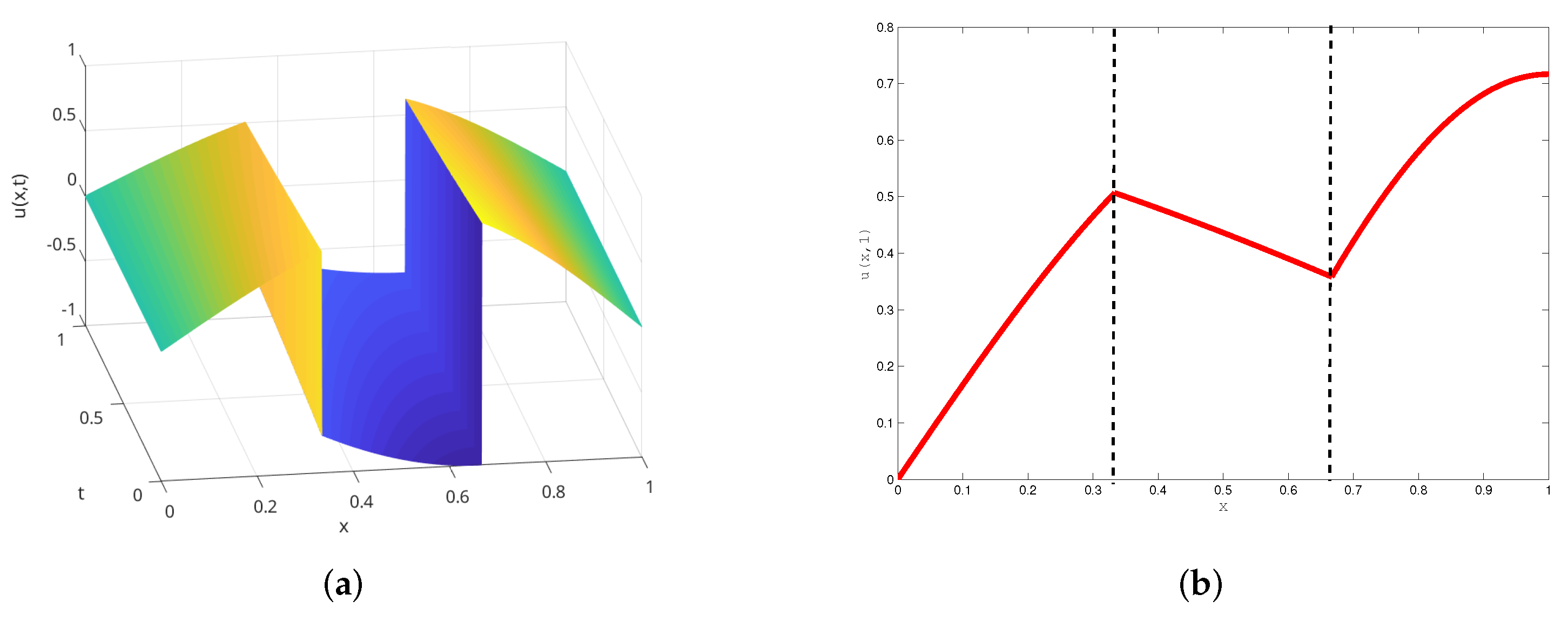
7. A Numerical Example

Let us consider that the physical and geometry parameters are given by

$$\begin{array}{cc}\hfill & L_0=0,L_1=1/3,L_2=2/3,L_3=1,C_1=C_2=C_3=1,\hfill \\ \hfill & {\tau }_q^{\left(1\right)}={\tau }_q^{\left(2\right)}={\tau }_q^{\left(3\right)}=1,{\tau }_T^{\left(1\right)}=1,{\tau }_T^{\left(2\right)}=4,{\tau }_T^{\left(3\right)}=2,\hfill \\ \hfill & k_1=8/27{\pi }^2,k_2=16/9{\pi }^2,k_3=4/9{\pi }^2,\mathrm{and} {\alpha }_1={\alpha }_2=1/2;\hfill \end{array}$$

the initial conditions are given by

$$\begin{array}{ccc}\hfill u(x,0)& {\displaystyle =\left\{\begin{array}{cc}sin(3\pi x/4),\hfill & 0\le x<L_1,\hfill \\ cos\left(\pi \right(x+2/3)/4),\hfill & L_1\le x<L_2,\hfill \\ sin\left(\pi \right(x-1/2\left)\right),\hfill & L_2\le x\le L_3,\hfill \end{array}\right.\frac{\partial u}{\partial t}(x,0)}& =-\frac{1}{3}u(x,0);\hfill \end{array}$$

and the boundary conditions are ${\phi }_1\left(t\right)=-3\pi exp(-t/3)/8$ and ${\phi }_2\left(t\right)=\pi exp(-t/3)/2.$ We observe that the analytic solution is given by

$$\begin{array}{cc}\hfill u(x,t)& =\left\{\begin{array}{cc}exp(-t/3)sin(3\pi x/4),\hfill & 0\le x<L_1,\hfill \\ exp(-t/3)cos\left(\pi \right(x+2/3)/4),\hfill & L_1\le x<L_2,\hfill \\ exp(-t/3)sin\left(\pi \right(x-1/2\left)\right),\hfill & L_2\le x\le L_3.\hfill \end{array}\right.\end{array}$$

We consider that the discretization parameters are $\Delta x_1=\Delta x_2=\Delta x$. Let us consider $\widehat{\mathbb{U}}=u(x,t)$ for $(x,t)\in Q_{\Delta x,\Delta t}$ (see Section 3.1), i.e., the evaluation of the analytical solution on the discretization domain; $\mathbb{U}$ the numerical solution; introduce the notation

$$\begin{array}{c}\hfill E_{\Delta x,\Delta t}={\parallel \widehat{\mathbb{U}}-\mathbb{U}\parallel }_{\infty },Orde{r}_x={log}_2\left(\frac{E_{2\Delta x,\Delta t}}{E_{\Delta x,\Delta t}}\right),Orde{r}_t={log}_2\left(\frac{E_{\Delta x,2\Delta t}}{E_{\Delta x,\Delta t}}\right),\end{array}$$

where ${\parallel ·\parallel }_{\infty }$ is the notation defined in (24)–(27). For the spatial convergence orders in the $L_{\infty }$-norm error, we consider several values of $\Delta x$ with fixed $\Delta t=1/1000$ and for the temporal convergence in the $L_{\infty }$-norm error, we consider several values of $\Delta t$ with fixed $\Delta x=1/1000$, the results of the simulation are shown on

Table 1. Convergence error. For space convergence, we fix $\Delta t=1/1000$. For temporal convergence we fix $\Delta x=1/1000$.

$\mathbf{\Delta }\mathit{x}$	${\mathit{E}}_{\mathbf{\Delta }\mathit{x},\mathbf{\Delta }\mathit{t}}$	${\mathit{Order}}_{\mathit{x}}$	$\mathbf{\Delta }\mathit{t}$	${\mathit{E}}_{\mathbf{\Delta }\mathit{x},\mathbf{\Delta }\mathit{t}}$	${\mathit{Order}}_{\mathit{t}}$
$0.1000$	$2.415\times {10}^{-4}$	-	$0.1000$	$4.688\times {10}^{-5}$	-
$0.0500$	$4.087\times {10}^{-5}$	$1.992$	$0.0500$	$2.257\times {10}^{-5}$	$2.000$
$0.0250$	$2.537\times {10}^{-5}$	$1.997$	$0.0250$	$3.762\times {10}^{-6}$	$2.001$
$0.0125$	$4.828\times {10}^{-6}$	$1.998$	$0.0125$	$6.276\times {10}^{-7}$	$2.002$

. The numerical solution is given on Figure 2.

8. Conclusions

In this paper, we have proposed a theoretical one-dimensional mathematical model for heat conduction model in a double-pane window with a temperature-jump boundary condition and a thermal lagging interfacial effect condition between layers. We construct a second-order accurate finite difference scheme and prove that finite difference scheme introduced is unconditionally stable, convergent, and has rate of convergence two in space and time for the $L_{\infty }$-norm.

References

1. Sahni, M.; Sahni, R. Applied Mathematical Modeling and Analysis in Renewable Energy, 1st ed.; CRC Press: Boca Raton, FL, USA, 2021. [Google Scholar]
2. Rashid, M.H. (Ed.) Electric Renewable Energy Systems; Elsevier: London, UK, 2015. [Google Scholar]
3. Arici, M.; Karabay, H.; Kan, M. Flow and heat transfer in double, triple and quadruple pane windows. Energy Build. 2015, 86, 394–402. [Google Scholar] [CrossRef]
4. Korpela, S.A.; Lee, Y.; Drummond, J.E. Heat Transfer Through a Double Pane Window. ASME J. Heat Transfer. 1982, 104, 539–544. [Google Scholar] [CrossRef]
5. Han, J.; Lu, L.; Yang, H. Numerical evaluation of the mixed convective heat transfer in a double-pane window integrated with see-through a-Si PV cells with low-e coatings. Appl. Energy 2010, 87, 3431–3437. [Google Scholar] [CrossRef]
6. Basok, B.I.; Davydenko, B.V.; Isaev, S.A.; Goncharuk, S.M.; Kuzhel, L.N. Numerical Modeling of Heat Transfer Through a Triple-Pane Window. J. Eng. Phys. Thermophys. 2016, 89, 1277–1283. [Google Scholar] [CrossRef]
7. Aydin, O. Conjugate heat transfer analysis of double pane windows. Build. Environ. 2006, 41, 109–116. [Google Scholar] [CrossRef]
8. Medved, S.; Novak, P. Heat transfer through a double pane window with an insulation screen open at the top. Energy Build. 1998, 28, 257–268. [Google Scholar] [CrossRef]
9. Chow, T.-T.; Li, C.; Lin, Z. Thermal characteristics of water-flow double-pane window. Int. J. Therm. Sci. 2011, 50, 140–148. [Google Scholar] [CrossRef]
10. Karabay, H.; Arıcı, M. Multiple pane window applications in various climatic regions of Turkey. Energy Build. 2012, 45, 67–71. [Google Scholar] [CrossRef]
11. Rubin, M. Calculating heat transfer through windows. Int. J. Energy Res. 1982, 6, 341–349. [Google Scholar] [CrossRef]
12. Aydin, O. Determination of optimum air-layer thickness in double-pane windows. Energy Build. 2000, 32, 303–308. [Google Scholar] [CrossRef]
13. Arici, M.; Karabay, H. Determination of optimum thickness of double-glazed windows for the climatic regions of Turkey. Energy Build. 2010, 42, 1773–1778. [Google Scholar] [CrossRef]
14. Arici, M.; Kan, M. An investigation of flow and conjugate heat transfer in multiple pane windows with respect to gap width, emissivity and gas filling. Renew. Energy 2015, 75, 249–256. [Google Scholar] [CrossRef]
15. Dorfman, A.; Renner, Z. Conjugate Problems in Convective Heat Transfer: Review. Math. Probl. Eng. 2009, 2009, 927350. [Google Scholar] [CrossRef]
16. Zudin, Y.B. Theory of Periodic Conjugate Heat Transfer, 2nd ed.; Springer: Berlin, Germany, 2011. [Google Scholar]
17. Kazemi-Kamyab, V.; van Zuijlen, A.H.; Bijl, H. A high order time-accurate loosely-coupled solution algorithm for unsteady conjugate heat transfer problems. Comput. Methods Appl. Mech. Eng. 2013, 264, 205–217. [Google Scholar] [CrossRef]
18. Ooi, E.H.; van Popov, V. An efficient hybrid BEM–RBIE method for solving conjugate heat transfer problems. Comput. Math. Appl. 2014, 66, 2489–2503. [Google Scholar] [CrossRef]
19. Costa, R.; Nóbrega, J.M.; Clain, S.; Machado, G.J. Very high-order accurate polygonal mesh finite volume scheme for conjugate heat transfer problems with curved interfaces and imperfect contacts. Comput. Methods Appl. Mech. Eng. 2019, 357, 112560. [Google Scholar] [CrossRef]
20. Pan, X.; Lee, C.; Choi, J.-I. Efficient monolithic projection method for time-dependent conjugate heat transfer problems. J. Comput. Phys. 2018, 369, 191–208. [Google Scholar] [CrossRef]
21. Guo, S.; Feng, Y.; Tao, W.-Q. Deviation analysis of loosely coupled quasi-static method for fluid-thermal interaction in hypersonic flows. Comput. Fluids 2017, 149, 194–204. [Google Scholar] [CrossRef]
22. Errera, M.-P.; Duchaine, F. Comparative study of coupling coefficients in Dirichlet-Robin procedure for fluid-structure aerothermal simulations. J. Comput. Phys. 2016, 312, 218–234. [Google Scholar] [CrossRef]
23. Kazemi-Kamyab, V.; van Zuijlen, A.H.; Bijl, H. Analysis and application of high order implicit Runge-Kutta schemes for unsteady conjugate heat transfer: A strongly-coupled approach. J. Comput. Phys. 2014, 272, 471–486. [Google Scholar] [CrossRef]
24. Dai, W.; Han, F.; Sun, Z. Accurate numerical method for solving dual-phase-lagging equation with temperature jump boundary condition in nano heat conduction. Int. J. Heat Mass Transf. 2013, 64, 966–975. [Google Scholar] [CrossRef]
25. Tzou, D.Y. A unified approach for heat conduction from macro-to micro-scale. ASME J. Heat Transf. 1995, 117, 8–16. [Google Scholar] [CrossRef]
26. Tzou, D.Y. Macro to Microscale Heat Transfer. The Lagging Behaviour, 2nd ed.; Taylor & Francis: Washington, DC, USA, 2014. [Google Scholar]
27. Sun, H.; Sun, Z.Z.; Dai, W. A second-order finite difference scheme for solving the dual-phase-lagging equation in a double-layered nano-scale thin film. Numer. Methods Partial. Differ. Equ. 2017, 33, 142–173. [Google Scholar] [CrossRef]
28. Ghazanfarian, J.; Abbassi, A. Effect of boundary phonon scattering on Dual-Phase-Lag model to simulate micro- and nano-scale heat conduction. Int. J. Heat And Mass Transf. 2009, 52, 3706–3711. [Google Scholar] [CrossRef]
29. Sun, Z.Z. Numerical Methods for Partial Differential Equations, 2nd ed.; Science Press: Beijing, China, 2012. [Google Scholar]
30. Liao, H.L.; Sun, Z.Z. Maximum norm error estimates of efficient difference schemes for second-order wave equations. J. Comput. Appl. Math. 2011, 235, 2217–2233. [Google Scholar] [CrossRef] [Green Version]
Figure 1. A schematic form of a a double-pane window.
Axioms 11 00422 g001
Figure 2. Numerical solution of the mathematical model (6)–(11) with the data of Section 7. (a) Full solution for for ( x , t ) [ 0 , 1 ] × [ 0 , 2 ] and (b) profile at T = 1 .
Axioms 11 00422 g002