
Modulation Transfer between Microwave Beams: A Hypothesized Case of a Classically-Forbidden Stochastic Process


Istituto di Fisica Applicata “Nello Carrara”, Consiglio Nazionale delle Ricerche, Via Madonna del Piano 10, 50019 Sesto Fiorentino, Italy
*
Author to whom correspondence should be addressed.
†
These authors contributed equally to this work.
Axioms 2022, 11(8), 416; https://doi.org/10.3390/axioms11080416
Submission received: 31 May 2022
/
Revised: 12 July 2022
/
Accepted: 17 August 2022
/
Published: 19 August 2022
(This article belongs to the Special Issue Advances in Stochastic Modelling)
Abstract
:Measurements of delay time in the transfer of modulation between a modulated to an unmodulated one, both of them derived by the same microwave source, are reported and interpreted. In the light of these results, the transfer of modulation can be hypothesized as due to a stochastic, classically-forbidden process, assisted by a photon–photon scattering mechanism.
MSC:
60H30; 62L201. Introduction
An unexpected transfer of modulation between microwave beams occurring in the region of the near field has been well demonstrated in previous [1,2] and even more recent papers [3,4]. In spite of the efforts so far made, a satisfying interpretation of this phenomenon is still lacking. In fact, while in the previous papers, a superluminal behavior was sustained on the basis of results obtained by a two-horn antenna experiment, in the more recent contributions, the role played by the stochastic processes has been hypothesized [3], especially in the light of delay-time measurements relative to the transfer of modulation [4].
Subsequently, we hypothesized that interference could be merely responsible for part of the transferred signal. Therefore, the experimental setup was modified in order to reduce spurious effects. The hypothesis of the stochastic nature of the involved process was thus confirmed as concomitant and co-operating with a photon–photon scattering mechanism [5]. In this framework, the temporal behavior turned out to be opposite to the previous one, that is—as will be demonstrated—decidedly subluminal. As far as we know, in the literature there are no other contributions on this topic, other than those we have already published. This holds true from both an experimental and a theoretical point of view.
2. Stochastic-Process Modeling
In this work, the second-order partial differential equation known as the telegrapher’s equation represents the starting point of the theoretical model presented. Originally, the telegrapher’s equation was used to model the current and voltage in a portion of a transmission line with distance and time. Since then, modern physics has exploited it in numerous applications from signal analysis [6,7,8,9,10], to random walk [11,12,13,14] and wave propagation [15,16,17].
Here, we are focused on a pioneering work by Kac [18], in which it was demonstrated that the telegrapher’s equation—a wave equation in the presence of dissipation—can be interpreted as being originated by zig-zag particle motion.
In particular, the equivalence between the telegrapher’s equation and a particle traveling in a straight line with constant velocity was established. In this model, the particle is characterized by a stochastic motion because it undergoes collisions that can reverse its velocity. After each step , the probability of reversing the velocity is , and it is for continuing in the same direction.
In the presence of dissipation, a randomized time replaces the time, and the displacement becomes .
The telegrapher’s equation is given by
where v is the propagation velocity in the x direction of the quantity (a field) and a is the dissipative parameter which is related to the jumping rate of the “particle” motion.
Subsequently, the problem was reconsidered by De Witt-Morette and Foong [19], who demonstrated that a solution to the telegrapher’s equation can be expressed by a quadrature as:
where is a solution of the wave equation without dissipation, Equation (1), with , and being arbitrary mixing coefficients so that .
Using Laplace transform analysis, for , can be expressed as follows [19,20]:
where is the Dirac function, the Heaviside step function and and the modified Bessel functions, respectively.
Moreover, by using asymptotic expansions of the Bessel functions and neglecting the contribution, Equation (3) can be expressed as the sum of two Gaussians. Thus, the two-variable function , as the density distribution of a randomized time r (t is the normal time), tends asymptotically for , to a Gaussian, with a standard deviation given by [20]. More exactly, results from the sum of two Gaussians, one centered at , the other at . In explicit form, we have
The importance of using a randomized time can be observed by calculating the average time [20,21]:
where is the traveled distance and v the velocity. This average can be regarded as a fictitious time that a particle would take to reach the average distance in the case of traveling with velocity v without reversal. By inverting Equation (5), the true time required to reach the distance L can be calculated.
Results of delay-time measurements show a rather unexpected, irregular behavior which reinforces the hypothesis of the presence of stochastic processes [4,5]. The shape of these data can be considered to be representative of the hypothesized zig-zag random paths. This fact induced us to consider, in the present case of near field propagation, an inversion of roles between r and t, in the sense that r becomes the observable (measurable) quantity, as typically occurs in a classically forbidden processes, as f.i. in the tunneling, where such as inversion was considered, at first, as a crude ansatz [21].
The novelty of the present approach is that the inversion of roles between the randomized time (r) and the normal time (t) represents the crucial point for the interpretation of the observed phenomenon, namely, the modulation transfer between microwave beams.
3. Experimental Set-Up
The procedure for time-delay measurements is similar to that described in reference [4]. The experimental set-up used is based on two crossing microwave beams emitted by two horn antennas [1,2]. Both beams were powered by the same generator at ∼9.3 GHz; the beam was modulated by a squared wave with a repetition frequency Ω of ∼800 Hz; the beam was unmodulated. The antenna responsible for the beam was placed at a suitable distance from the first one (as schematically shown in Figure 1): this beam was obtained as the near field emerging from a composed pupil [3,4] represented by a paraffin torus situated in the center of a circular aperture. The transferred modulation signal was detected by another small horn antenna placed in front of the launcher () at a variable distance ; see Figure 2. This third antenna was placed still beyond the region of interaction. Moreover, an absorber material was placed between the two launchers and in order to reduce their cross-talking [5]. The measurements were also performed by means of a lock-in amplifier tuned at the modulation frequency; the delay ones were performed over the rise or the fall time (of the order of nanoseconds) of the square wave. Accuracy of a few tens of picoseconds has been observed when using a temporal-resolution digital oscilloscope (Tektronik 2440 or TDS 680B). A number of determinations were obtained, and average between rise- and fall-time measurements were considered. The results are reported in Figure 3.
4. Results and Discussion
The results obtained for distance in the range of from 10 to 54 cm are shown in Figure 3. Each determination was obtained as an average between the rise- and fall-time measurements.
As anticipated, they showed an irregular behavior that supports the hypothesis of the existence of zig-zagging, random paths in the propagation. In the same graph, the dashed curve represents the function , being , computed by assuming s−1 and cm/ns, according to reference [4]. This curve represents the border line of the half area that contains the paths with a probability of ∼95%. The same curve represents , if we select a = 0.5 × 10⁹ s−1 and cm/s, and the probability will be reduced to ∼68%. Strictly speaking, these values should be valid only in the limit of , as indicated before Equation (4); outside this limit, the results are to be considered as purely indicative.
Under this assumption, an estimate of the extension of the average steps in the zig-zag paths could be obtained for , and for , we obtained [4,26]. This means that for s−1, ns and the corresponding cm, values that are in reasonable agreement with the observed variations in Figure 3.
If we maintain the ratio , we can evaluate as simply being given by
where is expressed in cm, a in s−1 and v in cm/ns.
Moreover, in Figure 3 are also plotted continuous curves of (OriginPro, Version 2018, OriginLab Corporation, Northampton, MA, USA). It is interesting to note that these curves reach the asymptotic values for cm.
However, reasonable agreement with the experimental data requires a smaller value of s−1. On the contrary, higher values of a could be acceptable only if we admit the presence of an offset in the data of about 1–2 ns. This hypothesis is not unrealistic, and the most important aspect in the data is the flattened behavior of their average. As anticipated since reference [4], noteworthy is the fact that in the considered case, and in this framework, we have an inversion of roles between r and t, since r becomes the observable quantity. Usually this occurs in classically-forbidden process, as f.i. in the tunneling [21]. This fact induced us to hypothesize, even in this case, the situation of a classically forbidden process.
However, in the present case, given by the expanded scale of time t in Figure 3, due to the low value of the velocity v in comparison to the light velocity, we have an evident sub-luminal behavior.
As for the origin of the transfer of modulation between the microwave beams, the abovementioned hypothesis of photon–photon scattering acting in the crossing area can be justified as follows [5]. The existence of a photonic rest mass, very small but not exactly zero, ∼ g [27], is not sufficient for supporting this hypothesis. However, in consideration of the relativistic relation [28]
where is the photon energy, v is the velocity and c is the light velocity in vacuum, we arrive at the following result. For , the mass m evidently becomes zero, but in our case, for GHz and , Equation (7) gives for m a (virtual) value of ∼ g, which would well support the scattering mechanism.
Therefore, it seems that, on the basis of this consideration, the hypothesis of the stochastic nature—and the one of the classically forbidden character—of the involved process becomes a more plausible one, in concomitance and cooperation with the scattering mechanism.
5. Conclusions and Perspectives
In this work, an unexpected transfer of modulation between two crossing microwave beams was measured in the region of the near field. Although this phenomenon has been already demonstrated in previous [1,2] and even relatively recent papers [3,4], a satisfying interpretation was still lacking. In fact, in previous papers, a superluminal behavior was sustained, and in the more recent one, a stochastic role was hypothesized. A modified experimental set-up was introduced herein in order to reduce spurious effects, and new experimental time-delay measurements are available. The hypothesis of the stochastic nature of the involved process was confirmed as co-operating with a photon–photon scattering mechanism [5]. Moreover, in this work, it was observed that the temporal behavior is decidedly subluminal, and this is the opposite to what was found in previous analysis. The novelty introduced here is represented by the inversion of roles between the randomized time (r) and the normal time (t), which is considered as crucial for the interpretation of the observed phenomenon, namely, the modulation transfer between microwave beams.
We also believe this topic should be further investigated from both experimental and theoretical point of view, and in particular, a different analysis could also benefit from other stochastic approaches, including Feynman’s transition elements [29] and nonstandard finite difference methods.
Author Contributions
Conceptualization, A.R. and I.C.; methodology, A.R. and I.C.; formal analysis, A.R. and I.C.; data curation, A.R. and I.C.; writing—original draft preparation, A.R. and I.C.; writing—review and editing, A.R. and I.C. All authors have read and agreed to the published version of the manuscript.
Funding
This research received no external funding.
Institutional Review Board Statement
Not applicable.
Informed Consent Statement
Not applicable.
Data Availability Statement
The data that support the findings of this study are available from the corresponding author upon reasonable request.
Conflicts of Interest
The authors declare no conflict of interest.
References
- Ranfagni, A.; Mugnai, D.; Ruggeri, R. Unexpected behavior of crossing microwave beams. Phys. Rev. E 2004, 69, 027601. [Google Scholar] [CrossRef] [PubMed]
- Ranfagni, A.; Mugnai, D. Superluminal behavior in the near field of crossing microwave beams. Phys. Lett. A 2004, 322, 146–149. [Google Scholar] [CrossRef]
- Cacciari, I.; Mugnai, D.; Ranfagni, A.; Petrucci, A. Cross-modulation between microwave beams interpreted as a stochastic process. Int. J. Mod. Phys. B 2021, 35, 2150037. [Google Scholar] [CrossRef]
- Cacciari, I.; Mugnai, D.; Ranfagni, A. Delay time in the tansfer of modulation between between microwave beams. Eng. Rep. 2021, 3, e12392. [Google Scholar]
- Cacciari, I.; Ranfagni, A. On the origin of the transfer of modulation between microwave beams. Mod. Phys. Lett. B 2022, 33, 2250096. [Google Scholar] [CrossRef]
- Jordan, P.M.; Puri, A. Digital signal propagation in dispersive media. J. Appl. Phys. 1999, 85, 1273–1282. [Google Scholar] [CrossRef]
- Ford, N.J.; Xiao, J.; Yan, Y. Stability of a Numerical Method for a space-time-fractional telegraph equation. Comput. Methods Appl. Math. 2015, 12, 273–288. [Google Scholar] [CrossRef]
- Stojanović, Z.; Čajić, E. Application of Telegraph Equation Solution Telecommunication Signal Transmission and Visualization in Matlab. In Proceedings of the 27th Telecommunications Forum (TELFOR), Belgrade, Serbia, 26–27 November 2019; pp. 1–4. [Google Scholar] [CrossRef]
- Minenna, D.F.G.; Terentyuk, A.G.; André, F.; Elskens, Y.; Ryskin, N.M. Recent discrete model for small-signal analysis of traveling-wave tubes. Phys. Scr. 2019, 94, 1–8. [Google Scholar] [CrossRef]
- Mokarram, A.; Abdipour, A.; Askarpour, A.N.; Mohammadzade, A.R. Time-domain signal and noise analysis of millimetre-wave/THz diodes by numerical solution of stochastic telegrapher’s equations. IET Microwaves Antennas Propag. 2020, 14, 1012–1020. [Google Scholar] [CrossRef]
- Banasiak, J.; Mika, J.R. Singular perturbed telegraph equations with applications in the random walk theory. J. Appl. Math. Stoch. Anal. 1998, 11, 9–28. [Google Scholar] [CrossRef]
- Weiss, G.H. Some applications of persistent random walks and the telegrapher’s equation. Phys. A Stat. Mech. Its Appl. 2002, 311, 381–410. [Google Scholar] [CrossRef]
- Garcia-Pelayo, R. The random flight and the persistent random walk. In Statistical Mechanics and Random Walks; Skogseid, A., Fasano, V., Eds.; Nova Science Publishers: New York, NY, USA, 2012; pp. 582–611. [Google Scholar]
- Masoliver, J. Telegraphic Transport Processes and Their Fractional Generalization: A Review and Some Extensions. Entropy 2021, 23, 364. [Google Scholar] [CrossRef] [PubMed]
- Weston, V.H.; He, S. Wave splitting of the telegraph equation in and its application to inverse scattering. Inverse Probl. 1993, 9, 789–812. [Google Scholar] [CrossRef]
- Sonnenschein, E.; Rutkevich, I.; Censor, D. Wave Packets and Group Velocity in Absorbing Media: Solutions of the Telegrapher’s Equation. Prog. Electromagn. Res. 2000, 27, 129–158. [Google Scholar] [CrossRef]
- Cáceres, M.O. Localization of plane waves in the stochastic telegrapher’s equation. Phys. Rev. E 2022, 105, 014110. [Google Scholar] [CrossRef]
- Kac, M. A Stochastic Model Related to the Telegrapher’s Equation. Rocky Mountain J. Math 1974, 4, 497–509. [Google Scholar] [CrossRef]
- DeWitt-Morette, C.; Foong, S.K. Path-integral solutions of wave equations with dissipation. Phys. Rev. Lett. 1989, 62, 2001–2004. [Google Scholar] [CrossRef]
- Foong, S.K. Kac’s Solution of the Telegrapher Equation (Part II). In Developments in General Relativity, Astrophysics and Quantum Theory: A Jubilee Volume in Honour of Nathan Rosen; Cooperstock, F.I., Horwitz, L.P., Rosen, J., Eds.; Institute of Physics: Bristol, UK, 1990; pp. 367–377. [Google Scholar]
- Mugnai, D.; Ranfagni, A.; Ruggeri, R.; Agresti, A. Semiclassical analysis of traversal time through Kac’s solution of the telegrapher’s equation. Phys. Rev. E 1994, 49, 1771–1774. [Google Scholar] [CrossRef]
- Sevimlican, A. An Approximation to Solution of Space and Time Fractional Telegraph Equations by He’s Variational Iteration Method. Math. Probl. Eng. 2010, 2010, 1–10. [Google Scholar] [CrossRef]
- Zhang, B.; Yu, W.; Mascagni, M. Revisiting Kac’s method: A Monte Carlo algorithm for solving the Telegrapher’s equations. Math. Comput. Simul. 2019, 156, 178–193. [Google Scholar] [CrossRef]
- Radice, M. One-dimensionale telegraphic process with noninstantaneous stochastic resetting. Phys. Rev. E 2021, 104, 044126. [Google Scholar] [CrossRef] [PubMed]
- Giona, M.; Cairoli, A.; Klages, R. Extended Poisson-Kac theory: A unifying framework for stochastic processes with finite propagation velocity. Phys. Rev. X 2022, 2, 021004. [Google Scholar] [CrossRef]
- Jacobson, T.; Schulman, L.S. Quantum stochastics: The passage from a relativistic to a non-relativistic path integral. J. Phys. A 1984, 17, 375–383. [Google Scholar] [CrossRef]
- Luo, J.; Tu, L.C.; Hu, Z.K.; Luan, E.J. New Experimental Limit on the Photon Rest Mass with a Rotating Torsion Balance. Phys. Rev. Lett. 2003, 90, 081801. [Google Scholar] [CrossRef] [PubMed]
- Toraldo di Francia, G. L’indagine del Mondo Fisico; Giulio Einaudi Ed: Torino, Italy, 1976; p. 338. [Google Scholar]
- Feynman, E.R.P.; Hibbs, A.R. Quantum Mechanics and Path Integrals; McGraw-Hill: New York, NY, USA, 1965; Chapter 7. [Google Scholar]
Figure 1.
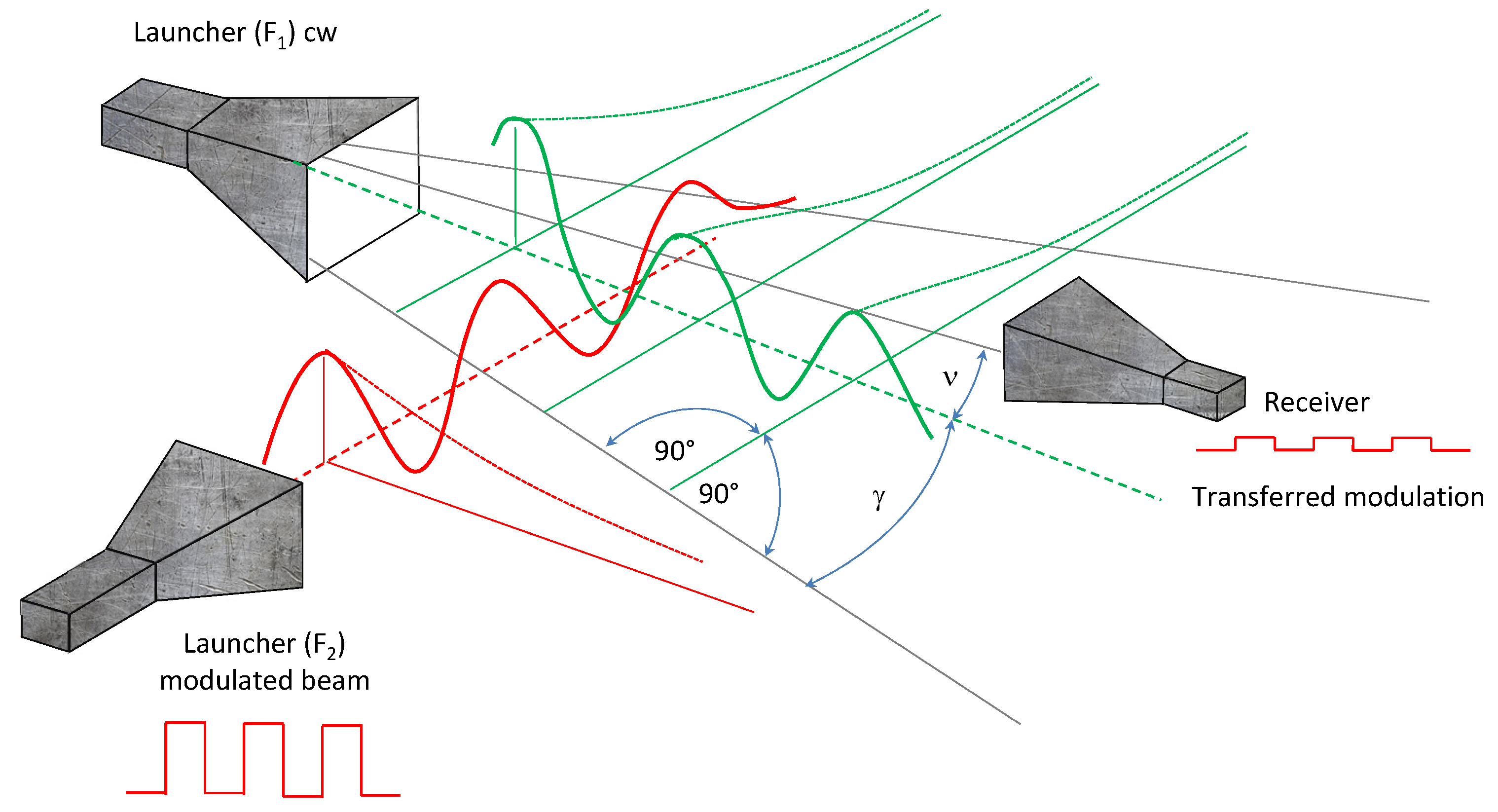
Artistic partial representation of the experimental setup, where is an angle of a few degrees, and is the half-fire angle of the horn antenna ( launcher), of 25 degrees. For clarity, the absorber between the two launchers ( and ) has been omitted.
Figure 1.
Artistic partial representation of the experimental setup, where is an angle of a few degrees, and is the half-fire angle of the horn antenna ( launcher), of 25 degrees. For clarity, the absorber between the two launchers ( and ) has been omitted.

Figure 2.
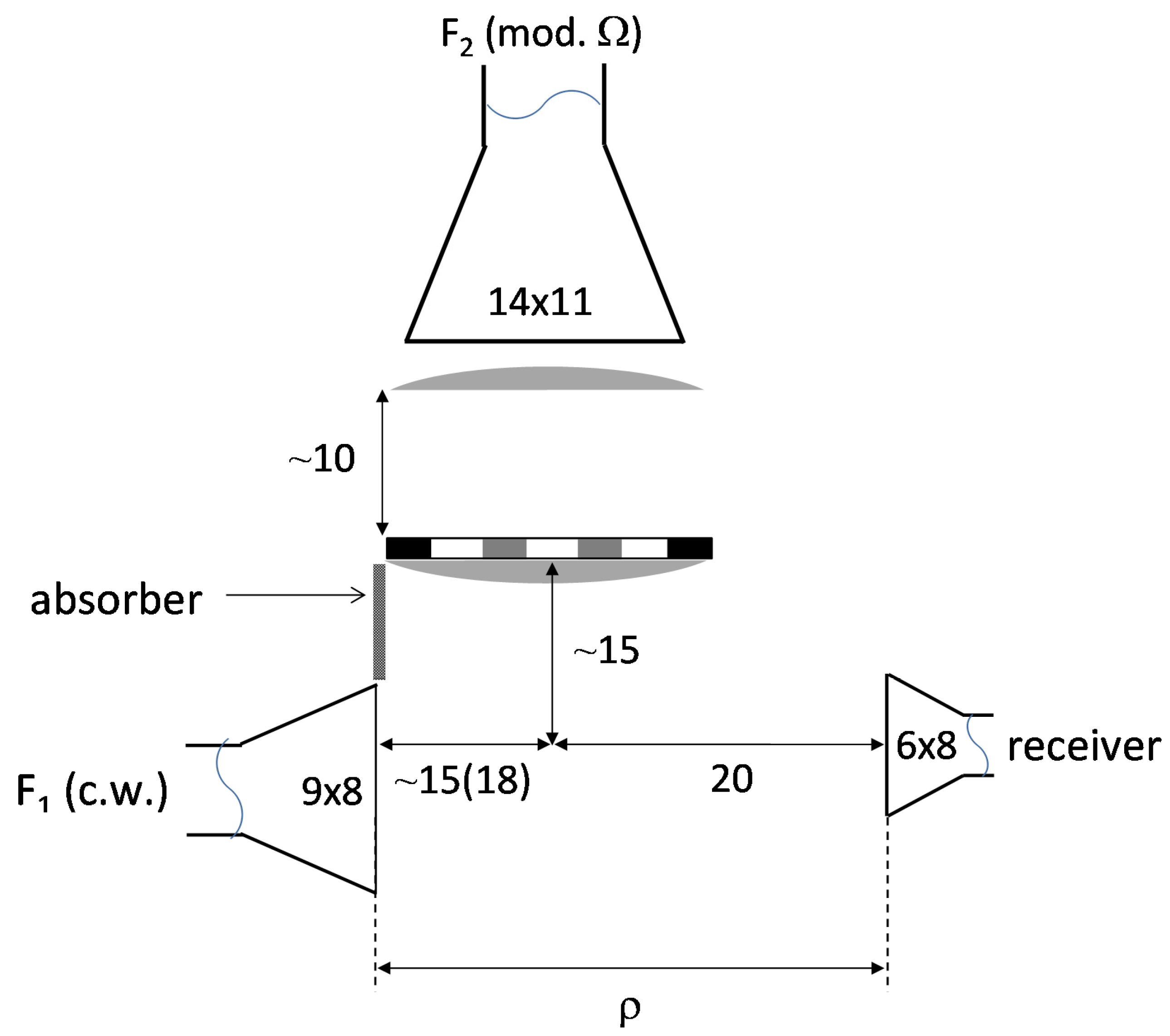
The experimental setup operated at 9.3 GHz. The typical geometry consisted of two horn antennas as launchers for the c.w. beam and the and Ω modulated beam, traveling through a composed pupil in order to reduce its width. The receiver horn antenna was placed at distance . An absorber material was suitably positioned between the launcher and in order to reduce their cross-talking [5]. All dimensions are expressed in centimeters.
Figure 2.
The experimental setup operated at 9.3 GHz. The typical geometry consisted of two horn antennas as launchers for the c.w. beam and the and Ω modulated beam, traveling through a composed pupil in order to reduce its width. The receiver horn antenna was placed at distance . An absorber material was suitably positioned between the launcher and in order to reduce their cross-talking [5]. All dimensions are expressed in centimeters.

Figure 3.
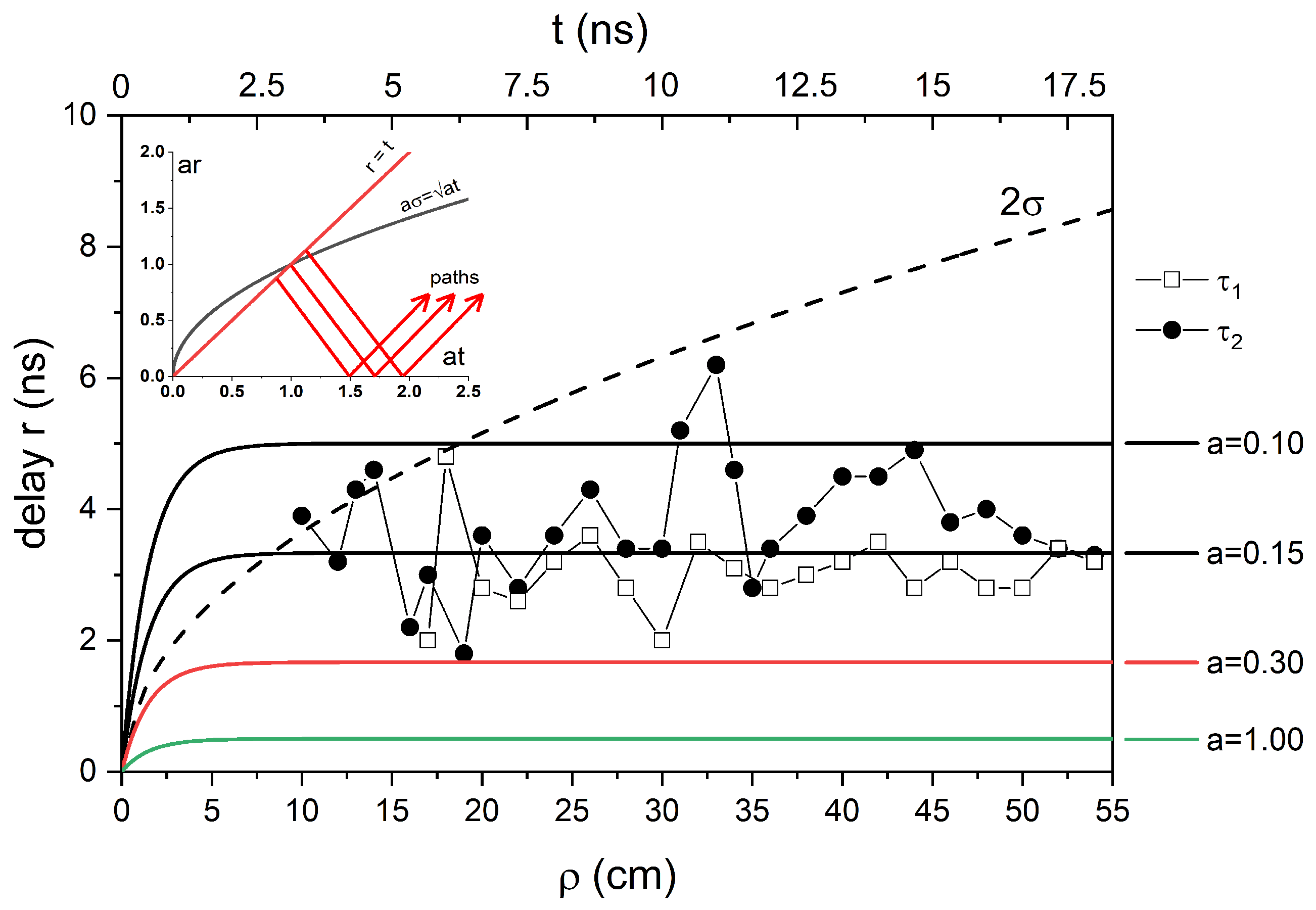
Two determinations of delay time, in the transfer of modulation between microwave beams, measured as a function of the distance between the launcher of the unmodulated beam and the receiver antenna, in the presence of the perpendicular modulated beam, are reported. The dashed curve represents and has been evaluated assuming ; and the continuous curves represent and have been computed by Equation (6) for some values of the parameter a, expressed in s−1. Hypothetical paths with reversals are given in the plane of the inset, after reference [4].
Figure 3.
Two determinations of delay time, in the transfer of modulation between microwave beams, measured as a function of the distance between the launcher of the unmodulated beam and the receiver antenna, in the presence of the perpendicular modulated beam, are reported. The dashed curve represents and has been evaluated assuming ; and the continuous curves represent and have been computed by Equation (6) for some values of the parameter a, expressed in s−1. Hypothetical paths with reversals are given in the plane of the inset, after reference [4].

Publisher’s Note: MDPI stays neutral with regard to jurisdictional claims in published maps and institutional affiliations. |
© 2022 by the authors. Licensee MDPI, Basel, Switzerland. This article is an open access article distributed under the terms and conditions of the Creative Commons Attribution (CC BY) license (https://creativecommons.org/licenses/by/4.0/).
Share and Cite
MDPI and ACS Style
Ranfagni, A.; Cacciari, I. Modulation Transfer between Microwave Beams: A Hypothesized Case of a Classically-Forbidden Stochastic Process. Axioms 2022, 11, 416. https://doi.org/10.3390/axioms11080416
AMA Style
Ranfagni A, Cacciari I. Modulation Transfer between Microwave Beams: A Hypothesized Case of a Classically-Forbidden Stochastic Process. Axioms. 2022; 11(8):416. https://doi.org/10.3390/axioms11080416
Chicago/Turabian StyleRanfagni, Anedio, and Ilaria Cacciari. 2022. "Modulation Transfer between Microwave Beams: A Hypothesized Case of a Classically-Forbidden Stochastic Process" Axioms 11, no. 8: 416. https://doi.org/10.3390/axioms11080416
Note that from the first issue of 2016, this journal uses article numbers instead of page numbers. See further details here.