Fractional Dynamics of a Measles Epidemic Model

Abstract

In this work, we replaced the integer derivative with Caputo derivative to model the transmission dynamics of measles in an epidemic situation. We began by recalling some results on the local and global stability of the measles-free equilibrium point as well as the local stability of the endemic equilibrium point. We computed the basic reproduction number of the fractional model and found that is it equal to the one in the integer model when the fractional order ν = 1. We then performed a sensitivity analysis using the global method. Indeed, we computed the partial rank correlation coefficient (PRCC) between each model parameter and the basic reproduction number R₀ as well as each variable state. We then demonstrated that the fractional model admits a unique solution and that it is globally stable using the Ulam–Hyers stability criterion. Simulations using the Adams-type predictor–corrector iterative scheme were conducted to validate our theoretical results and to see the impact of the variation of the fractional order on the quantitative disease dynamics.

1. Introduction

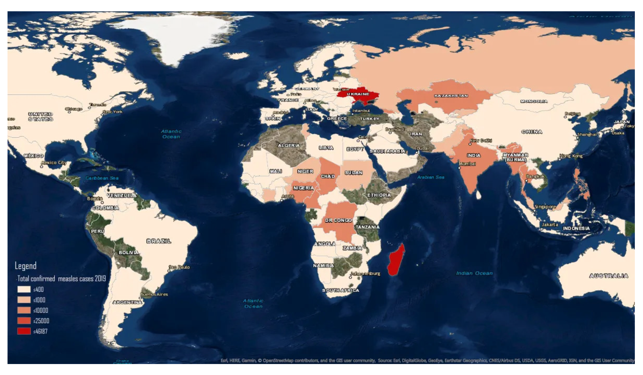
Measles, also called rubeola or morbilli, is an infectious illness caused by the Morbillivirus of the family of Paramyxoviridae [1,2]. It principally affects children below five years of age and has high mortality [2,3]. Despite the availability of a vaccine against the measles virus, this illness remained a health problem that concerns the World Health Organization (WHO). Indeed, in 2017, about 110,000 people died from measles, particularly children below the age of 6 [2,4]. Table 1 depicts the 10 countries that have mainly been affected by a global measles outbreak, while Figure 1 shows the global repartition of measles.

Several works based on mathematical modeling have been proposed to study the transmission dynamics of several diseases. These works are mainly based on the SIR-type compartmental modeling [5,6,7,8,9,10,11,12]. The interest in using mathematical modeling to study the measles transmission dynamics and to find control measures that permit preventing or stopping measles outbreaks is increasing [13]. Many authors have proposed and analyzed different mathematical models of measles based on compartmental modeling [2,14,15,16,17,18,19,20,21,22]. Among these works, only [2] took into account the effects of hospitalization of the infected individuals. Indeed, most of them consider the traditional SEIR-compartmental models.

Table 1. Top 10 countries with global measles outbreaks [23].

Rank	Country	Number of Cases	Rank	Country	Number of Cases
1	Nigeria	17,794	6	Democratic Republic of the Congo	1907
2	India	5874	7	Afghanistan	1621
3	Somalia	4772	8	Liberia	1495
4	Ethiopia	3403	9	Cameroon	1373
5	Pakistan	2677	10	Ivory Coast	1152

Table 1. Top 10 countries with global measles outbreaks [23].

Rank	Country	Number of Cases	Rank	Country	Number of Cases
1	Nigeria	17,794	6	Democratic Republic of the Congo	1907
2	India	5874	7	Afghanistan	1621
3	Somalia	4772	8	Liberia	1495
4	Ethiopia	3403	9	Cameroon	1373
5	Pakistan	2677	10	Ivory Coast	1152

Figure 1. World repartition of measles in 2019 [24].

Figure 1. World repartition of measles in 2019 [24].

Fractional calculus has been a useful tool to model, predict, and forecast epidemic outbreaks for the last 20 years. Indeed, as fractional calculus was predicted by Leibniz to be a paradox, it has become a central interest for many researchers in various fields, such as engineering sciences [25], mathematical epidemiology [26,27], physics [28], and economics [29]. The most commonly known fractional operators are Caputo derivatives and their variants [30,31,32,33,34,35,36,37,38], the Caputo–Fabrizio derivative [39], Atangana–Baleanu derivative [40,41], and piece-wise derivative [42]. The kernels of some of these mentioned operators have different characteristics. For example, the Caputo operator is defined with the power law-type kernel (nonlocal but singular), and that of Caputo–Fabrizio has an exponentially decaying (nonsingular) kernel, while the Atangana–Baleanu operator in the Caputo sense has a Mittag–Leffler-type kernel [43]. In a recent work [44], Atangana formulated and studied a compartmental model that could be used to depict the survival of fractional calculus. The fact that the Caputo operator has a memory effect and the Caputo derivative of a constant function is equal to zero [45] means that this derivative is the most used.

Concerning the transmission dynamics of measles, few authors have used fractional derivatives [22,46,47,48,49]. In [46]. Farman et al. employed a fraction Caputo operator on a SEIR epidemic model to control measles for infected populations. Ogunmiloro et al. [47] studied a mathematical model describing the transmission dynamics of measles with a double vaccination dose, treatment, and two groups of measles-infected and measles-induced encephalitis-infected humans with relapse under the fractional Atangana–Baleanu–Caputo (ABC) operator. Qureshi, in [22], proposed a new epidemiological system for the measles epidemic using the Caputo fractional derivative with a memory effect.

The objective of this work was to compare, from a quantitative point of view, the dynamics of an epidemic model of measles with integer derivatives and fractional derivatives (in the sense of Caputo). To achieve our goal, we extended the model by Olumuyiwa et al. [2], which consists of a six-compartmental model integrating vaccinated and hospitalized individuals, by replacing the integer derivative with the Caputo derivative. The theoretical analysis of the fractional model was performed by a classical method and consists of the algebraic determination of the basic reproduction number $R_0$, which depends on the fractional order $\nu$, the proof of the local and global stabilities of the disease-free equilibrium, as well as the local stability of the endemic equilibrium. To determine the model parameters that have a great influence on the measles epidemic in Nigeria, we performed a global sensitivity analysis of the model by computing the partial rank correlation coefficients between the basic reproduction number (as well as state variables) and the model parameters. We proved the existence and uniqueness of the solutions of the fractional model as well as its global stability using the Ulam–Hyers method. We then constructed a numerical scheme based on the Adams-type predictor–corrector iterative scheme [50,51], and finally, performed a numerical simulation to see the impact of the variation of the fractional order on the disease dynamics.

The paper is presented as follows: Section 2 is devoted to the model formulation and basic results. Section 3 is devoted to the global sensitivity analysis. In Section 4, we recall some definitions and useful results concerning fractional calculus. We also formulated the fractional measles model with the Caputo derivative and performed asymptotic stability of equilibrium points. Then, we provide the proof of existence, the uniqueness of the solution, and the global stability of the fractional model. The numerical scheme is also presented in this section. Section 5 is devoted to the numerical simulations. A conclusion rounds up the paper.

2. Model Formulation and Basic Results

In [2], Olumuyiwa et al. proposed and studied the following $\mathcal{S}\mathcal{V}\mathcal{E}\mathcal{I}\mathcal{H}\mathcal{R}$ compartmental model with the integer derivative

$$\left\{\begin{array}{ccc}{\displaystyle \frac{d}{dt}}\mathcal{S}\left(t\right)\hfill & =\hfill & \mathsf{\Lambda }+\alpha \mathcal{V}-\beta \mathcal{S}\mathcal{I}-\stackrel{k_1}{\overbrace{(c+d)}}\mathcal{S},\hfill \\ {\displaystyle \frac{d}{dt}}\mathcal{V}\left(t\right)\hfill & =\hfill & c\mathcal{S}-\stackrel{k_2}{\overbrace{(d+\alpha )}}\mathcal{V},\hfill \\ {\displaystyle \frac{d}{dt}}\mathcal{E}\left(t\right)\hfill & =\hfill & \beta \mathcal{S}\mathcal{I}-\stackrel{k_3}{\overbrace{(d+\gamma )}}\mathcal{E},\hfill \\ {\displaystyle \frac{d}{dt}}\mathcal{I}\left(t\right)\hfill & =\hfill & \gamma \mathcal{E}-\stackrel{k_4}{\overbrace{(d+a+\varphi )}}\mathcal{I},\hfill \\ {\displaystyle \frac{d}{dt}}\mathcal{H}\left(t\right)\hfill & =\hfill & \varphi \mathcal{I}-\stackrel{k_5}{\overbrace{(\sigma +a+d)}}\mathcal{H},\hfill \\ {\displaystyle \frac{d}{dt}}\mathcal{R}\left(t\right)\hfill & =\hfill & \sigma \mathcal{H}-d\mathcal{R}.\hfill \end{array}\right.$$

(1)

to model the transmission dynamics of measles in Nigeria. In Equation (1), $\mathcal{S}$ denotes the susceptible population, $\mathcal{V}$ is the vaccinated population, $\mathcal{E}$ is the total number of latent persons (infected but not infectious), $\mathcal{I}$ is the total number of infected persons, $\mathcal{H}$ is the total number of hospitalized persons, and $\mathcal{R}$ is the total number of recovered persons. The description of the model parameters and their values are consigned in

Table 2. Biological description of model parameters and their numerical values [2].

Parameter	Description	Values (per Week)
$\mathsf{\Lambda }$	Recruitment rate	68,027
$\alpha$	Rate of loss of vaccine immunity	$0.003286$
$\beta$	Transmission Rate	${10}^{-9}$
c	Vaccination rate	${10}^{-6}$
d	Natural death rate	$0.000309$
$\gamma$	Rate of progression from $\mathcal{E}$ to $\mathcal{I}$	$0.5$
a	Disease-induced rate	$0.033720$
$\varphi$	Rate of progression from $\mathcal{I}$ to $\mathcal{H}$	$0.036246$
$\sigma$	Rate of progression from $\mathcal{H}$ to $\mathcal{R}$	$0.062366$

.

The following subset of ${\mathbb{R}}^6$

$$\Sigma =\left\{{\left(\mathcal{S},\mathcal{V},\mathcal{E},\mathcal{I},\mathcal{H},\mathcal{R}\right)}^t\in {\mathbb{R}}_{+}^6:\mathcal{N}:=\mathcal{S}+\mathcal{V}+\mathcal{E}+\mathcal{I}+\mathcal{H}+\mathcal{R}\le {\displaystyle \frac{\mathsf{\Lambda }}{d}}\right\}$$

is positively invariant for system Equation (2), which defines a dynamical system. Since the state variable $\mathcal{R}$ only appears in the last equation of Equation (1), it is sufficient to study the following reduced system

$$\left\{\begin{array}{ccc}{\displaystyle \frac{d}{dt}}\mathcal{S}\left(t\right)\hfill & =\hfill & \mathsf{\Lambda }+\alpha \mathcal{V}-\beta \mathcal{S}\mathcal{I}-\stackrel{k_1}{\overbrace{(c+d)}}\mathcal{S},\hfill \\ {\displaystyle \frac{d}{dt}}\mathcal{V}\left(t\right)\hfill & =\hfill & c\mathcal{S}-\stackrel{k_2}{\overbrace{(d+\alpha )}}\mathcal{V},\hfill \\ {\displaystyle \frac{d}{dt}}\mathcal{E}\left(t\right)\hfill & =\hfill & \beta \mathcal{S}\mathcal{I}-\stackrel{k_3}{\overbrace{(d+\gamma )}}\mathcal{E},\hfill \\ {\displaystyle \frac{d}{dt}}\mathcal{I}\left(t\right)\hfill & =\hfill & \gamma \mathcal{E}-\stackrel{k_4}{\overbrace{(d+a+\varphi )}}\mathcal{I},\hfill \\ {\displaystyle \frac{d}{dt}}\mathcal{H}\left(t\right)\hfill & =\hfill & \varphi \mathcal{I}-\stackrel{k_5}{\overbrace{(\sigma +a+d)}}\mathcal{H}.\hfill \end{array}\right.$$

(2)

The model Equation (2) admits two nonnegative equilibrium points: the disease-free equilibrium ${\mathbb{E}}_0={\left({\mathcal{S}}_0,{\mathcal{V}}_0,0,0,0,0\right)}^t={\left({\displaystyle \frac{(d+\alpha )\mathsf{\Lambda }}{(d+\alpha +c)d}},{\displaystyle \frac{c\mathsf{\Lambda }}{(d+\alpha +c)d}},0,0,0,0\right)}^t$ and a unique endemic equilibrium ${\mathbb{E}}_1={\left({\mathcal{S}}_1,{\mathcal{V}}_1,{\mathcal{E}}_1,{\mathcal{I}}_1,{\mathcal{H}}_1,{\mathcal{R}}_1\right)}^t$, where

$$\left\{\begin{array}{ccc}{\mathcal{I}}_1\hfill & =\hfill & {\displaystyle \frac{\mathsf{\Lambda }\gamma }{R_0{k}_3{k}_4}}\left(R_0-1\right),\hfill \\ {\mathcal{S}}_1\hfill & =\hfill & {\displaystyle \frac{k_2\mathsf{\Lambda }}{c\alpha +k_2(k_1+\beta {\mathcal{I}}_1)}},\hfill \\ {\mathcal{V}}_1\hfill & =\hfill & {\displaystyle \frac{c}{k_2}}{\mathcal{S}}_1,\hfill \\ {\mathcal{E}}_1\hfill & =\hfill & {\displaystyle \frac{\beta }{k_3}}{\mathcal{S}}_1{\mathcal{I}}_1,\hfill \\ {\mathcal{H}}_1\hfill & =\hfill & {\displaystyle \frac{\varphi }{k_5}}{\mathcal{I}}_1,\hfill \end{array}\right.$$

(3)

with $R_0$, which denotes the basic reproduction number expressed as follows:

$$R_0={\displaystyle \frac{\beta \gamma }{k_3{k}_4}}{\displaystyle \frac{(d+\alpha )\mathsf{\Lambda }}{(d+\alpha +c)d}}.$$

(4)

From Equation (3), it follows that:

Proposition 1.

The model Equation (2) admits a unique endemic equilibrium point ${\mathbb{E}}_1={\left({\mathcal{S}}_1,{\mathcal{V}}_1,{\mathcal{E}}_1,{\mathcal{I}}_1,{\mathcal{H}}_1,{\mathcal{R}}_1\right)}^t$ if and only if $R_0>1$.

Theorem 1

([2]). (i) The disease-free equilibrium point ${\mathbb{E}}_0$ is locally and globally asymptotically stable if and only if $R_0\le 1$;

(ii) 

The unique endemic equilibrium point ${\mathbb{E}}_1$ is locally stable whenever $R_0>1$.

Remark 1.

As suggested in [44], the epidemic spread can also be evaluated by computing the so-called threshold “strength number”. Indeed, the strength number permits knowing, in an epidemic period, if there is the possibility for a renewal process [44]. In the case of epidemic measles, model Equation (9), this threshold is equal to zero, which implies that the spread does not have a renewal process.

3. Uncertainty and Global Sensitivity Analysis

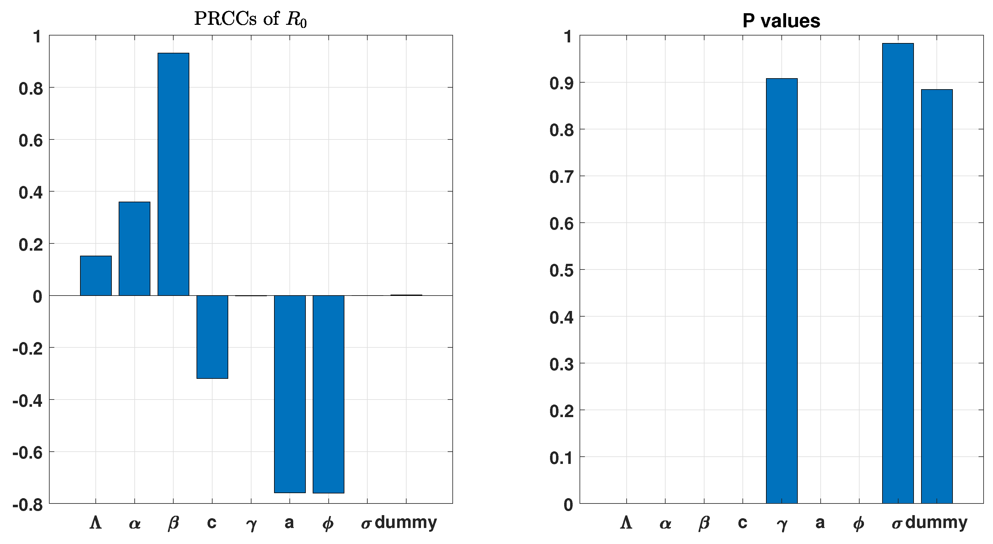
In [2], the authors performed a local sensitivity analysis by computing the sensitivity indices of $R_0$ against model parameters. The disadvantage of this kind of sensitivity analysis (SA) is that the sensitivity index is calculated by varying only one parameter while the remaining parameters are fixed. Considering the combined variability from all input parameters simultaneously, we performed a global sensitivity analysis to examine the model’s response to parameter variation in the parameter space. To this aim, we computed the partial rank correlation coefficient (PRCC) between $R_0$ (as well as each state variable of the model) and each model parameter. PRCC is the best and most reliable sensitivity analysis method that provides monotonicity between parameters and the model output when we want to measure the nonlinear (but monotonic) relationship between two variables [52,53]. The Latin hypercube sampling (LHS) was used as a sampling technique [54] with the number of runs equal to 5000. Each model parameter was supposed to be random with uniform distribution and their mean values are listed in Table 2. The most influential parameter is the one with the PRCC less than $-0.5$ or greater than $+0.5$ [53]. The results of the SA are depicted in Figure 2, Figure 3 and Figure 4.

From Figure 2, it is clear that the parameters $\beta$, a, and $\varphi$ have the highest influence on $R_0$. This suggests that individual protection combined with efficient treatment may potentially be the most effective strategy to reduce the basic reproduction number.

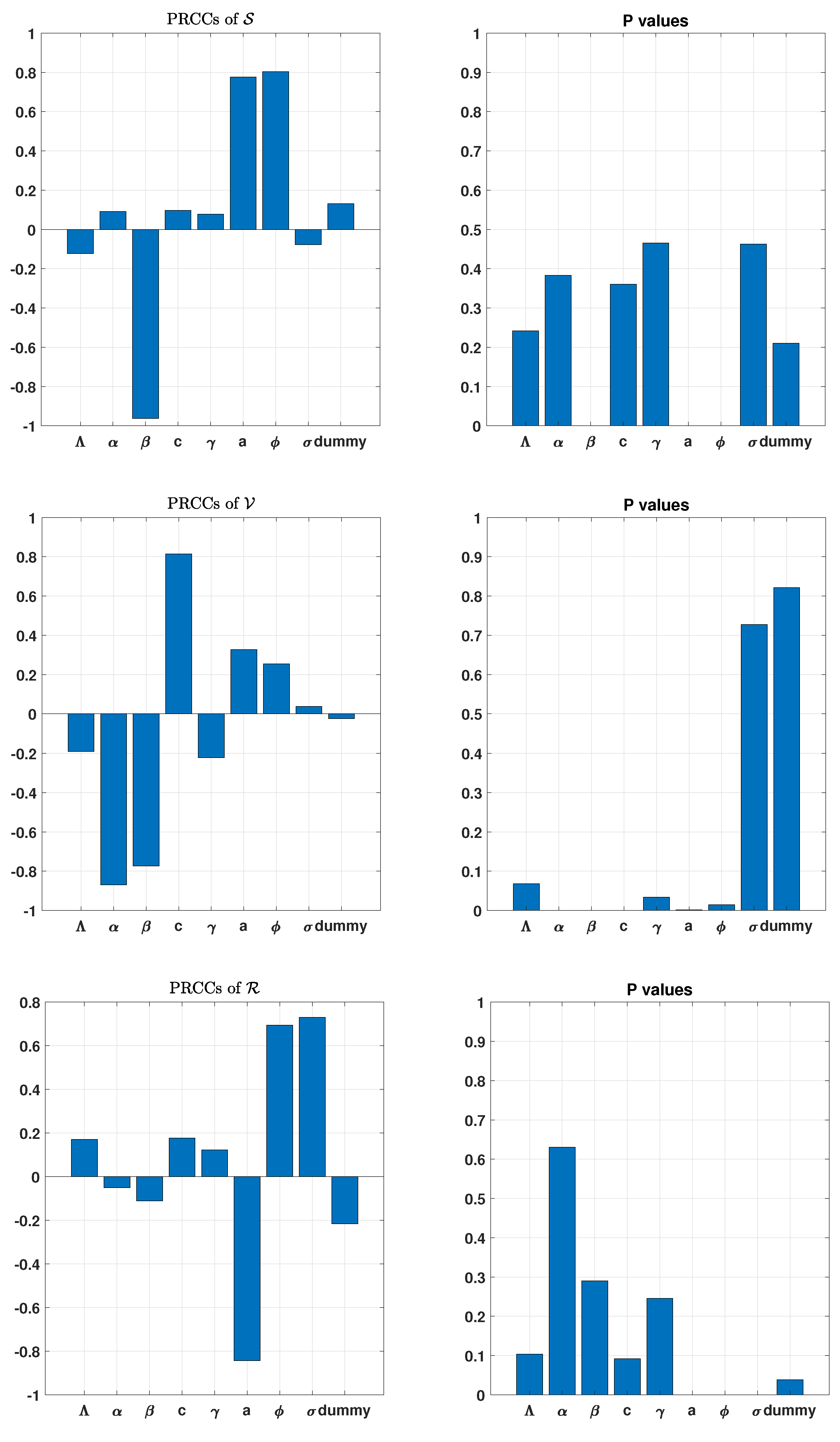
From Figure 3, the parameters with the highest influence on $\mathcal{S}$ are $\beta$, a, and $\varphi$; the ones with the highest influence on $\mathcal{V}$ are $\beta$, $\alpha$, and c, while the ones with the highest influence on $\mathcal{R}$ are a, $\varphi$, and $\sigma$.

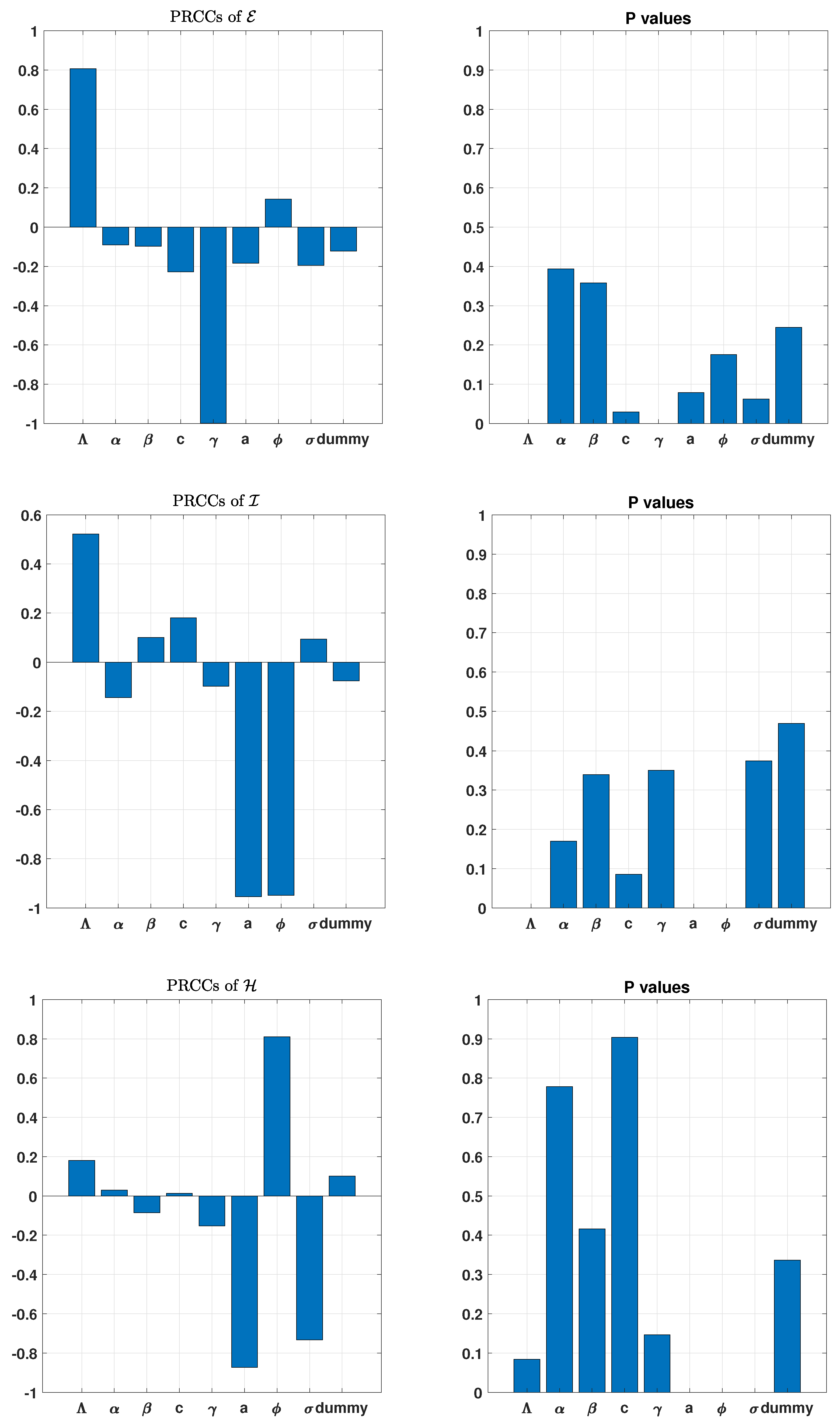
From Figure 4, the parameters with the highest influence on $\mathcal{E}$ are $\mathsf{\Lambda }$ and $\gamma$; the ones with the highest influence on $\mathcal{I}$ are $\mathsf{\Lambda }$, a, and $\varphi$, while the ones with the highest influence on $\mathcal{H}$ are a, $\varphi$, and $\sigma$. In general, mass vaccination combined with personal protection and care as soon as the first symptoms appear would make it possible to effectively fight measles.

4. The Fractional Model and Its Analysis

4.1. Primarily Definition and Results of Fractional Calculus

Now, we present some main properties of the fractional-order differential equations.

Definition 1

([55,56]). The Caputo fractional derivative of a function $f\in \mathcal{C}\left([a,b],\mathbb{R}\right)$ can be written as follows:

$${}_0^C{\mathbb{D}}_t^{\nu }\psi \left(t\right)={\chi }^{\mu -\nu }{f}^{\left(\mu \right)}\left(t\right),\beta >0,$$

(5)

where ${}_0^C{\mathbb{D}}^{\nu }$ is the Caputo operator, $0<\nu \le 1$ is the fractional order, μ is the smallest integer not equal to ν, and ${\chi }^{\varphi }$ is the Riemann–Liouville integral operator of order ϕ, defined as follows

$${\chi }^{\varphi }\mathsf{{\rm Y}}\left(t\right)=\frac{1}{\mathsf{\Gamma }\left(\varphi \right)}{\int }_0^t{(t-\tau )}^{\varphi -1}\mathsf{{\rm Y}}\left(\tau \right)\mu \tau ,\varphi >0.$$

(6)

Theorem 2

([55,57]). Consider the m-dimensional system

$$\left\{\begin{array}{ccc}\frac{{\theta }^{\nu }z}{\theta t^{\nu }}\hfill & =\hfill & \omega z,\hfill \\ z\left(0\right)\hfill & =\hfill & z_0,\hfill \end{array}\right.$$

(7)

where ω is a squared constant matrix of order $m\times m$, and $0<\nu <1$. Let us denote by ${\gamma }_i$, $i=1,2,...,m$ the eigenvalues of ω.

• $|arg\left({\gamma }_i\right)|>\frac{\nu \pi }{2}$, $i=1,2,\dots ,m$ iff $z=0$ is asymptotically stable;
• $z=0$ is stable if $\left|arg\left({\gamma }_i\right)\right|\ge \frac{\nu \pi }{2}$, $i=1,2,\dots ,m$, and eigenvalues with $\left|arg\left({\gamma }_i\right)\right|=\frac{\nu \pi }{2}$ have the same algebraic and geometric multiplicities.

Theorem 3

([55,57]). Let us consider the following system:

$$\left\{\begin{array}{ccc}\frac{{\mu }^{\nu }z}{\mu t^{\nu }}\hfill & =\hfill & \mathsf{\Psi }\left(z\right),\hfill \\ z\left(0\right)\hfill & =\hfill & z_0 with 0<\nu <1 and z\in {\mathbb{R}}^{\nu }.\hfill \end{array}\right.$$

(8)

Solving equation $\mathsf{\Psi }\left(z\right)=0$ permits obtaining the equilibrium points of system Equation (8). If all of the eigenvalues ${\gamma }_i$ of $J=\frac{\partial \psi \left(z^{*}\right)}{\partial z}$ satisfy $\left|arg\left({\gamma }_i\right)\right|>\frac{\nu \pi }{2}$, then the equilibrium point $z^{*}$ is locally asymptotically stable (LAS).

4.2. The Fractional Model with Caputo Operator

By replacing integer derivative with Caputo fractional derivative in system (1), we obtain the following system:

$$\left\{\begin{array}{ccc}{}_0^C{\mathbb{D}}^{\nu }\mathcal{S}\left(t\right)\hfill & =\hfill & {\mathsf{\Lambda }}^{\nu }+{\alpha }^{\nu }\mathcal{V}-{\beta }^{\nu }\mathcal{S}\mathcal{I}-(c^{\nu }+d^{\nu })\mathcal{S},\hfill \\ {}_0^C{\mathbb{D}}^{\nu }\mathcal{V}\left(t\right)\hfill & =\hfill & c^{\nu }\mathcal{S}-(d^{\nu }+{\alpha }^{\nu })\mathcal{V},\hfill \\ {}_0^C{\mathbb{D}}^{\nu }\mathcal{E}\left(t\right)\hfill & =\hfill & {\beta }^{\nu }\mathcal{S}\mathcal{I}-(d^{\nu }+{\gamma }^{\nu })\mathcal{E},\hfill \\ {}_0^C{\mathbb{D}}^{\nu }\mathcal{I}\left(t\right)\hfill & =\hfill & {\gamma }^{\nu }\mathcal{E}-(d^{\nu }+a^{\nu }+{\varphi }^{\nu })\mathcal{I},\hfill \\ {}_0^C{\mathbb{D}}^{\nu }\mathcal{H}\left(t\right)\hfill & =\hfill & {\varphi }^{\nu }\mathcal{I}-({\sigma }^{\nu }+a^{\nu }+d^{\nu })\mathcal{H},\hfill \\ {}_0^C{\mathbb{D}}^{\nu }\mathcal{R}\left(t\right)\hfill & =\hfill & {\sigma }^{\nu }\mathcal{H}-d^{\nu }\mathcal{R},\hfill \end{array}\right.$$

(9)

For this model, the corresponding basic reproduction number is given by

$$R_0={\displaystyle \frac{{\beta }^{\nu }{\gamma }^{\nu }(d^{\nu }+{\alpha }^{\nu }){\mathsf{\Lambda }}^{\nu }}{(d^{\nu }+{\gamma }^{\nu })(d^{\nu }+a^{\nu }+{\varphi }^{\nu })(d^{\nu }+{\alpha }^{\nu }+c^{\nu })d^{\nu }}}.$$

(10)

From Equation (10), we note that for $\nu =1$, the basic reproduction number coincides for both models.

As in the case of the model with the integer derivative Equation (2), the fractional model Equation (4) only has one endemic equilibrium ${\mathbb{E}}_1={\left({\mathcal{S}}_1,{\mathcal{V}}_1,{\mathcal{E}}_1,{\mathcal{I}}_1,{\mathcal{H}}_1,{\mathcal{R}}_1\right)}^{\prime }$, where

$$\left\{\begin{array}{ccc}{\mathcal{I}}_1\hfill & =\hfill & {\displaystyle \frac{{\mathsf{\Lambda }}^{\nu }{\gamma }^{\nu }}{R_0{k}_3{k}_4}}\left(R_0-1\right),{\mathcal{S}}_1={\displaystyle \frac{(d^{\nu }+{\alpha }^{\nu }){\mathsf{\Lambda }}^{\nu }}{c\alpha +k_2(k_1+{\beta }^{\nu }{\mathcal{I}}_1)}},\hfill \\ {\mathcal{V}}_1\hfill & =\hfill & {\displaystyle \frac{c^{\nu }}{k_2}}{\mathcal{S}}_1,{\mathcal{E}}_1={\displaystyle \frac{{\beta }^{\nu }}{k_3}}{\mathcal{S}}_1{\mathcal{I}}_1,{\mathcal{H}}_1={\displaystyle \frac{{\varphi }^{\nu }}{k_5}}{\mathcal{I}}_1,{\mathcal{R}}_1={\displaystyle \frac{{\sigma }^{\nu }}{d^{\nu }}}{\mathcal{H}}_1,\hfill \end{array}\right.$$

(11)

with Setting $k_1=c^{\nu }+d^{\nu }$, $k_2=d^{\nu }+{\alpha }^{\nu }$, $k_3=d^{\nu }+{\gamma }^{\nu }$, $k_4=d^{\nu }+a^{\nu }+{\varphi }^{\nu }$, and $k_5={\sigma }^{\nu }+a^{\nu }+d^{\nu }$.

4.2.1. Asymptotic Stability of the Disease-Free Equilibrium

The following theorems are proved in the same way as in [2].

Theorem 4.

The disease-free equilibrium point ${\mathbb{E}}_0$ is locally asymptotically stable if $R_0<1$; otherwise, it is unstable.

Theorem 5.

The disease-free equilibrium point $\left({\mathbb{E}}_0\right)$ is globally asymptotically stable whenever $R_0<1$.

Theorem 6.

The endemic equilibrium point $\left({\mathbb{E}}_1\right)$ is locally stable, when $R_0>1$.

4.2.2. Existence and Uniqueness of Solution

In this section, we present the results of the existence and uniqueness of the solution of the fractional differential Equation (9).

For this purpose, let $\eta =\mathcal{C}\left([0;a],\mathbb{R}\right)$, a Banach space of the continuous function from $[0;a]$ to $\mathbb{R}$, endowed with the norm ${\Vert \mathcal{Z}\Vert }_{\eta }=\underset{t\in \left[0,a\right]}{sup}\left\{\left|\mathcal{Z}\right|\right\}$.

The system Equation (9) can be rewritten in the following compact form:

$${}_t^C\mathbb{D}\mathcal{X}\left(t\right)=\xi \left(t,\mathcal{X}\right),\mathcal{X}\left(0\right)={\mathcal{X}}_0\ge 0,t\in [0,a],\nu \in (0;1).$$

(12)

where $\mathcal{X}={\left(\mathcal{S},\mathcal{V},\mathcal{E},\mathcal{I},\mathcal{R}\right)}^{\prime }$ and $\xi ={\left({\xi }_1,{\xi }_2,{\xi }_3,{\xi }_4,{\xi }_5,{\xi }_6\right)}^{\prime }$ with

$$\left\{\begin{array}{c}{\xi }_1={\mathsf{\Lambda }}^{\nu }+{\alpha }^{\nu }\mathcal{V}-{\beta }^{\nu }\mathcal{S}\mathcal{I}-(c^{\nu }+d^{\nu })\mathcal{S},\hfill \\ {\xi }_2=c^{\nu }\mathcal{S}-(d^{\nu }+{\alpha }^{\nu })\mathcal{V},\hfill \\ {\xi }_3={\beta }^{\nu }\mathcal{S}\mathcal{I}-(d^{\nu }+{\gamma }^{\nu })\mathcal{E},\hfill \\ {\xi }_4={\gamma }^{\nu }\mathcal{E}-(d^{\nu }+a^{\nu }+{\varphi }^{\nu })\mathcal{I},\hfill \\ {\xi }_5={\varphi }^{\nu }\mathcal{I}-({\sigma }^{\nu }+a^{\nu }+d^{\nu })\mathcal{H},\hfill \\ {\xi }_6={\sigma }^{\nu }\mathcal{H}-d^{\nu }\mathcal{R},\hfill \end{array}\right.$$

Since ${\xi }_i\in \eta$, for all of $i\in [0;6]\cap \mathbb{N}$, then the following operator

$$\left(\mathcal{P}\mathcal{X}\right)\left(t\right)={\mathcal{X}}_0+{\displaystyle \frac{1}{\mathsf{\Gamma }\left(\nu \right)}}{\int }_0^t{\left(t-\alpha \right)}^{\nu -1}\xi \left(\alpha ,\mathcal{X}\left(\alpha \right)\right)d\alpha ,$$

(13)

is well-defined. The following result is valid:

Lemma 1.

Let $\overline{\mathcal{X}}={(\overline{\mathcal{S}},\overline{\mathcal{V}},\overline{\mathcal{E}},\overline{\mathcal{I}},\overline{\mathcal{H}},\overline{\mathcal{R}})}^{\prime }$. The function $\xi ={\left({\xi }_i\right)}^{\prime }$ defined above satisfies

$\Vert \xi (t,\mathcal{X}\left(t\right))-\xi (t,\overline{\mathcal{X}}\left(t\right)){\Vert }_{\eta }\le {\mathbf{N}}_{\xi }{\Vert \mathcal{X}-\overline{\mathcal{X}}\Vert }_{\eta }$ for some ${\mathbf{N}}_{\xi }>0$.

Proof. 

We proceed as follows for the first component of $\xi$:

$$\begin{array}{cc}\hfill & \left|{\xi }_1(t,\mathcal{X}\left(t\right))-{\xi }_1(t,\overline{\mathcal{X}}\left(t\right))\right|\hfill \\ \hfill & =\left|{\alpha }^{\nu }(\mathcal{V}\left(t\right)-\overline{\mathcal{V}}\left(t\right))-{\beta }^{\nu }(\mathcal{S}\left(t\right)\mathcal{I}\left(t\right)-\overline{\mathcal{S}}\left(t\right)\overline{\mathcal{I}}\left(t\right))-h_1(\mathcal{S}\left(t\right)-\overline{\mathcal{S}}\left(t\right))\right|,\hfill \\ \hfill & \le h_1\left|\mathcal{S}\left(t\right)-\overline{\mathcal{S}}\left(t\right)\right|+{\alpha }^{\nu }\left|\mathcal{V}\left(t\right)-\overline{\mathcal{V}}\left(t\right)\right|+{\beta }^{\nu }\left|\mathcal{S}\left(t\right)\mathcal{I}\left(t\right)-\overline{\mathcal{S}}\left(t\right)\overline{\mathcal{I}}\left(t\right)\right|.\hfill \end{array}$$

(14)

However,

$$\begin{array}{cc}\hfill \left|\mathcal{S}\left(t\right)\mathcal{I}\left(t\right)-\overline{\mathcal{S}}\left(t\right)\overline{\mathcal{I}}\left(t\right)\right|& =\left|\mathcal{I}\left(t\right)\left(\mathcal{S}\left(t\right)-\overline{\mathcal{S}}\left(t\right)\right)+\overline{\mathcal{S}}\left(t\right)\left(\mathcal{I}\left(t\right)-\overline{\mathcal{I}}\left(t\right)\right)\right|\hfill \\ & \le \left|\mathcal{I}\left(t\right)\right|\left|\mathcal{S}\left(t\right)-\overline{\mathcal{S}}\left(t\right)\right|+\left|\overline{\mathcal{S}}\left(t\right)\right|\left|\mathcal{I}\left(t\right)-\overline{\mathcal{I}}\left(t\right)\right|.\hfill \end{array}$$

Thus, we obtain

$$\begin{array}{cc}\hfill & \left|{\xi }_1(t,\mathcal{X}\left(t\right))-{\xi }_1(t,\overline{\mathcal{X}}\left(t\right))\right|\hfill \\ \hfill & =\left|{\alpha }^{\nu }(\mathcal{V}\left(t\right)-\overline{\mathcal{V}}\left(t\right))-{\beta }^{\nu }(\mathcal{S}\left(t\right)\mathcal{I}\left(t\right)-\overline{\mathcal{S}}\left(t\right)\overline{\mathcal{I}}\left(t\right))-h_1(\mathcal{S}\left(t\right)-\overline{\mathcal{S}}\left(t\right))\right|,\hfill \\ \hfill & \le h_1\left|\mathcal{S}\left(t\right)-\overline{\mathcal{S}}\left(t\right)\right|+{\alpha }^{\nu }\left|\mathcal{V}\left(t\right)-\overline{\mathcal{V}}\left(t\right)\right|\hfill \\ \hfill & +{\beta }^{\nu }\left(\left|\mathcal{I}\left(t\right)\right|\left|\mathcal{S}\left(t\right)-\overline{\mathcal{S}}\left(t\right)\right|+\left|\overline{\mathcal{S}}\left(t\right)\right|\left|\mathcal{I}\left(t\right)-\overline{\mathcal{I}}\left(t\right)\right|\right)\hfill \\ \hfill & =\left(h_1+{\beta }^{\nu }\left|\mathcal{I}\left(t\right)\right|\right)\left|\mathcal{S}\left(t\right)-\overline{\mathcal{S}}\left(t\right)\right|+{\alpha }^{\nu }\left|\mathcal{V}\left(t\right)-\overline{\mathcal{V}}\left(t\right)\right|\hfill \\ \hfill & +{\beta }^{\nu }\left|\overline{\mathcal{S}}\left(t\right)\right|\left|\mathcal{I}\left(t\right)-\overline{\mathcal{I}}\left(t\right)\right|\hfill \\ \hfill & \le {\mathbf{N}}_1\left(\left|\mathcal{S}\left(t\right)-\overline{\mathcal{S}}\left(t\right)\right|+\left|\mathcal{V}\left(t\right)-\overline{\mathcal{V}}\left(t\right)\right|+\left|\mathcal{I}\left(t\right)-\overline{\mathcal{I}}\left(t\right)\right|\right),\hfill \end{array}$$

(15)

where ${\mathbf{N}}_1=h_1+{\alpha }^{\nu }+\underset{t\in \left[0,a\right]}{max}\left\{{\beta }^{\nu }\left|\mathcal{I}\left(t\right)\right|+{\beta }^{\nu }\left|\overline{\mathcal{S}}\left(t\right)\right|\right\}$, with $h_1=c^{\nu }+d^{\nu }$.

Similarly, with ${\xi }_2$, we also have:

$$\begin{array}{cc}\hfill \left|{\xi }_2(t,\mathcal{X}\left(t\right))-{\xi }_2(t,\overline{\mathcal{X}}\left(t\right))\right|& =\left|c^{\nu }(\mathcal{S}\left(t\right)-\overline{\mathcal{S}}\left(t\right))-h_2(\mathcal{V}\left(t\right)-\overline{\mathcal{V}}\left(t\right))\right|,\hfill \\ \hfill & \le c^{\nu }\left|(\mathcal{S}\left(t\right)-\overline{\mathcal{S}}\left(t\right))\right|+h_2\left|(\mathcal{V}\left(t\right)-\overline{\mathcal{V}}\left(t\right))\right|\hfill \\ \hfill & \le {\mathbf{N}}_2\left(\left|\mathcal{S}\left(t\right)-\overline{\mathcal{S}}\left(t\right)\right|+\left|\mathcal{V}\left(t\right)-\overline{\mathcal{V}}\left(t\right)\right|\right),\hfill \end{array}$$

(16)

where ${\mathbf{N}}_2=c^{\nu }+h_2$, where $h_2=d^{\nu }+{\alpha }^{\nu }$.

Based on the analogous reasoning, we obtain ${\xi }_i$, $i\in [0;6]\cap \mathcal{N}$:

$$\begin{array}{cc}\hfill \left|{\xi }_3(t,\mathcal{X}\left(t\right))-{\xi }_3(t,\overline{\mathcal{X}}\left(t\right))\right|& \le {\mathbf{N}}_3\left(\left|\mathcal{S}\left(t\right)-\overline{\mathcal{S}}\left(t\right)\right|+\left|\mathcal{I}\left(t\right)-\overline{\mathcal{I}}\left(t\right)\right|+\left|\mathcal{E}\left(t\right)-\overline{\mathcal{E}}\left(t\right)\right|\right),\hfill \\ \hfill \left|{\xi }_4(t,\mathcal{X}\left(t\right))-{\xi }_4(t,\overline{\mathcal{X}}\left(t\right)\right|& \le {\mathbf{N}}_4\left(\left|\mathcal{E}\left(t\right)-\overline{\mathcal{E}}\left(t\right)\right|+\left|\mathcal{I}\left(t\right)-\overline{\mathcal{I}}\left(t\right)\right|\right),\hfill \\ \hfill \left|{\xi }_5(t,\mathcal{X}\left(t\right)-{\xi }_5(t,\overline{\mathcal{X}}\left(t\right)\right|& \le {\mathbf{N}}_5\left(\left|\mathcal{I}\left(t\right)-\overline{\mathcal{I}}(t\right|+\left|\mathcal{H}\left(t\right)-\overline{\mathcal{H}}\left(t\right)\right|\right),\hfill \\ \hfill \left|{\xi }_6(t,\mathcal{X}\left(t\right))-{\xi }_6(t,\overline{\mathcal{X}Y}\left(t\right))\right|& \le {\mathbf{N}}_6\left(\left|\mathcal{H}\left(t\right)-\overline{\mathcal{H}}\left(t\right)\right|+\left|\mathcal{R}\left(t\right)-\overline{\mathcal{R}}\left(t\right)\right|\right),\hfill \end{array}$$

(17)

where ${\mathbf{N}}_3=h_3+\underset{t\in \left[0,a\right]}{max}\left\{{\beta }^{\nu }\left(\left|\mathcal{I}\right|+\left|\overline{\mathcal{S}}\right|\right)\right\}$, ${\mathbf{N}}_4={\gamma }^{\nu }+h_4$, ${\mathbf{N}}_5={\varphi }^{\nu }+h_5$, ${\mathbf{N}}_6={\varphi }^{\nu }+d^{\nu }$ with $h_3=d^{\nu }-{\gamma }^{\nu }$,$h_4=d^{\nu }+a^{\nu }+{\varphi }^{\nu }$, $h_5={\sigma }^{\nu }+a^{\nu }+d^{\nu }$.

Therefore, we finally obtain

$$\begin{array}{cc}\hfill \Vert \xi (t,\mathcal{X}\left(t\right))-\xi (t,\overline{\mathcal{X}}\left(t\right)){\Vert }_{\eta }& =su{p}_{t\in \left[0;a\right]}\sum _{i=1}^6\left|{\xi }_i(t,\mathcal{X}\left(t\right))-{\xi }_i(t,\overline{\mathcal{X}}\left(t\right))\right|,\hfill \\ & \le \stackrel{{\mathbf{N}}_{\eta }}{\overbrace{\left({\mathbf{N}}_1+{\mathbf{N}}_2+{\mathbf{N}}_3+{\mathbf{N}}_4+{\mathbf{N}}_5+{\mathbf{N}}_6\right)}}{\Vert \mathcal{X}-\overline{\mathcal{X}}\Vert }_{\eta }.\hfill \end{array}$$

□

Theorem 7.

Let the result of Lemma 1 hold and $\varpi ={\displaystyle \frac{a^{\nu }}{\mathsf{\Gamma }(\nu +1)}}$. If $\varpi {\mathbf{N}}_{\eta }<1$, then there exists a unique solution of the model Equation (12) on $\left[0,a\right]$, which is uniformly Lyapunov-stable.

Proof. 

The function $\xi :\left[0,a\right]\times {\mathbb{R}}^6\to {\mathbb{R}}_{+}^6$ is clearly continuous in its domain. Thus, the existence of the solutions to Equations (9) and (12) follows from (Theorem 3.1, [58]).

The Banach contraction mapping principle on operator $\mathcal{P}$ (see Equation (13)) will be used in the following to prove the uniqueness of the solution of the fractional model Equation (12). By definition, $\underset{t\in \left[0,a\right]}{sup}\Vert \xi (t,0)\Vert ={\mathsf{\Lambda }}^{\nu }$. Let us now define $\zeta >{\displaystyle \frac{\Vert {\mathcal{X}}_0\Vert +\varpi {\mathsf{\Lambda }}^{\nu }}{1-\varpi {\mathbf{N}}_{\eta }}}$ and a closed convex set ${\mathcal{Z}}_{\zeta }=\left\{\mathcal{X}\in {\eta :\Vert \mathcal{X}\Vert }_{\eta }\le \zeta \right\}$. Thus, for the sel- map property, it suffices to show that $\mathcal{P}{\mathcal{Z}}_{\zeta }\subseteq {\mathcal{Z}}_{\zeta }$. Let $\mathcal{X}\in {\mathcal{Z}}_{\zeta }$, we have

$$\begin{array}{cc}\hfill {\Vert \mathcal{P}\mathcal{X}\Vert }_{\eta }& =\underset{t\in \left[0,a\right]}{sup}\left\{\left|{\mathcal{X}}_0+{\displaystyle \frac{1}{\mathsf{\Gamma }\left(\nu \right)}}{\int }_0^t{(t-\epsilon )}^{\nu -1}\xi \left(\epsilon ,\mathcal{X}\left(\epsilon \right)\right)d\epsilon \right|\right\},\hfill \\ & \le \left|{\mathcal{X}}_0\right|+{\displaystyle \frac{1}{\mathsf{\Gamma }\left(\nu \right)}}\underset{t\in \left[0,a\right]}{sup}\left\{{\int }_0^t{(t-\epsilon )}^{\nu -1}\left(\left|\xi \left(\epsilon ,\mathcal{X}\left(\epsilon \right)\right)-\xi (\epsilon ,0)\right|+\left|\xi (\epsilon ,0)\right|\right)d\epsilon \right\},\hfill \\ & \le \left|{\mathcal{X}}_0\right|+{\displaystyle \frac{1}{\mathsf{\Gamma }\left(\nu \right)}}\underset{t\in \left[0,a\right]}{sup}\left\{{\int }_0^t{(t-\epsilon )}^{\nu -1}{(\Vert \xi (\epsilon ,\mathcal{X}\left(\epsilon \right))-\xi (\epsilon ,0)\Vert }_{\eta }+{\Vert \xi (\epsilon ,0)\Vert }_{\eta })d\epsilon \right\},\hfill \\ & \le \left|{\mathcal{X}}_0\right|+{\displaystyle \frac{{\mathbf{N}}_{\eta }{\Vert \mathcal{X}\Vert }_{\eta }+{\mathsf{\Lambda }}^{\nu }}{\mathsf{\Gamma }\left(\nu \right)}}\underset{t\in \left[0,a\right]}{sup}\left\{{\int }_0^t{(t-\epsilon )}^{\nu -1}d\epsilon \right\},\hfill \\ & \le \left|{\mathcal{X}}_0\right|+{\displaystyle \frac{{\mathbf{N}}_{\eta }\zeta +{\mathsf{\Lambda }}^{\nu }}{\mathsf{\Gamma }\left(\nu \right)}}\underset{t\in \left[0,a\right]}{sup}\left\{{\int }_0^t{(t-\epsilon )}^{\nu -1}d\epsilon \right\},\hfill \\ & =\left|{\mathcal{X}}_0\right|+{\displaystyle \frac{a^{\nu }}{\mathsf{\Gamma }(\nu +1)}}\left({\mathbf{N}}_{\eta }\zeta +{\mathsf{\Lambda }}^{\nu }\right),\hfill \\ & =\left|{\mathcal{X}}_0\right|+\varpi ({\mathbf{N}}_{\eta }\zeta +{\mathsf{\Lambda }}^{\nu }),\hfill \\ & \le \zeta .\hfill \end{array}$$

□

Then, $\mathcal{P}\mathcal{X}\subseteq {\mathcal{Z}}_{\zeta }$ and $\mathcal{P}$ are indeed the self-map. It remains to show that $\mathcal{P}$ is a contraction. Let $\mathcal{X}$ and $\overline{\mathcal{X}}$ two solutions of Equation (12). Using the result of Lemma 1, we obtain

$$\begin{array}{cc}\hfill \Vert \mathcal{P}\mathcal{X}-\mathcal{P}\overline{\mathcal{X}}{\Vert }_{\eta }& =\underset{t\in \left[0,a\right]}{sup}\left\{\left|\left(\mathcal{P}\mathcal{X}\right)\left(t\right)-\left(\mathcal{P}\overline{\mathcal{X}}\right)\left(t\right)\right|\right\},\hfill \\ & ={\displaystyle \frac{1}{\mathsf{\Gamma }\left(\nu \right)}}\underset{t\in \left[0,a\right]}{sup}\left\{{\int }_0^t{(t-\epsilon )}^{\nu -1}\left|\xi (\epsilon ,\mathcal{X}\left(\epsilon \right))-\xi (\epsilon ,\overline{\mathcal{X}}\left(\epsilon \right))\right|d\epsilon \right\},\hfill \\ & \le {\displaystyle \frac{{\mathbf{N}}_{\eta }}{\mathsf{\Gamma }\left(\nu \right)}}\underset{t\in \left[0,a\right]}{sup}\left\{{\int }_0^t{(t-\epsilon )}^{\nu -1}(\left|\mathcal{X}\left(\epsilon \right)-\overline{\mathcal{X}}\left(\epsilon \right)\right|d\epsilon \right\},\hfill \\ & \le \varpi {\mathbf{N}}_{\eta }{\Vert \mathcal{X}-\overline{\mathcal{X}}\Vert }_{\eta }.\hfill \end{array}$$

The condition $\varpi N_{\eta }<1$ ensures that $\mathcal{P}$ is a contraction mapping. Thus, by the Banach contraction mapping principle, $\mathcal{P}$ has a unique fixed point on $\left[0,a\right]$, which is the solution of Equation (12). Theorem 3.2 in [58] ensures the uniformly Lyapunov stability of the solution.

4.3. Global Stability of the Fractional Model

In what follows, we will perform the global stability of the fractional-order model Equation (9) in the sense of Ulam–Hyers [59,60]. To this aim, we introduce the following inequality:

$$\left|{}_0^C{\mathbb{D}}^{\nu }\mathcal{X}\left(t\right)-\xi (t,\mathcal{X}\left(t\right))\right|\le b,t\in [0;a].$$

(18)

A function $\overline{\mathcal{X}}\in \eta$ is a solution of Equation (18) if there exists $\aleph \in \eta$ satisfying

• $\left|\aleph \left(t\right)\right|\le b$;
• ${}_0^C{\mathbb{D}}^{\nu }\overline{\mathcal{X}}\left(t\right)=\xi (t,\overline{\mathcal{X}}\left(t\right))+\aleph \left(t\right)$, $t\in [0;a]$.

Since $\overline{\mathcal{X}}\in \eta$ is a solution of Equation (18), then $\overline{\mathcal{X}}\in \eta$ is also a solution of the following integral inequality

$$\left|\overline{\mathcal{X}}\left(t\right)-\overline{\mathcal{X}}\left(0\right)-{\displaystyle \frac{1}{\mathsf{\Gamma }\left(\nu \right)}}{\int }_0^t{(t-ϵ)}^{\nu -1}\xi (ϵ,\overline{\mathcal{X}}\left(ϵ\right))dϵ\right|\le \varpi b.$$

(19)

We claim the following result:

Theorem 8.

Assume that the result of Lemma 1 holds, and $1-\varpi {\mathbf{N}}_{\eta }>0$ with $\varpi ={\displaystyle \frac{a^{\nu }}{\mathsf{\Gamma }(\nu +1)}}$. The fractional order model Equation (9) (and equivalently Equation (12)) is Ulam–Hyers-stable and, consequently, generalized Ulam–Hyers-stable.

Proof. 

Let $\mathcal{X}$ be a unique solution of Equation (12), and $\overline{\mathcal{X}}$ satisfies Equation (18). For $b>0$, $t\in [0,a]$, we have

$$\begin{array}{cc}\hfill \Vert \overline{\mathcal{X}}{\left(t\right)-\mathcal{X}\left(t\right)\Vert }_{\eta }& =\underset{t\in [0,a]}{sup}\left|\overline{\mathcal{X}}\left(t\right)-\mathcal{X}\left(t\right)\right|\hfill \\ & =\underset{t\in [0,a]}{sup}\left|\overline{\mathcal{X}}\left(t\right)-\mathcal{X}\left(0\right)-{\displaystyle \frac{1}{\mathsf{\Gamma }\left(\nu \right)}}{\int }_0^t{(t-ϵ)}^{\nu -1}\xi (ϵ,\mathcal{X}\left(ϵ\right))dϵ\right|\hfill \\ & \le \underset{t\in [0,a]}{sup}\left|\overline{\mathcal{X}}\left(t\right)-\overline{\mathcal{X}}\left(0\right)-{\displaystyle \frac{1}{\mathsf{\Gamma }\left(\nu \right)}}{\int }_0^t{(t-ϵ)}^{\nu -1}\xi (ϵ,\overline{\mathcal{X}}\left(ϵ\right))dϵ\right|\hfill \\ & +\underset{t\in [0,a]}{sup}{\displaystyle \frac{1}{\mathsf{\Gamma }\left(\nu \right)}}{\int }_0^t{(t-ϵ)}^{\nu -1}\left|\xi (ϵ,\overline{\mathcal{X}}\left(ϵ\right))-\xi (ϵ,\mathcal{X}\left(ϵ\right))\right|dϵ\hfill \\ & \le \varpi b+{\displaystyle \frac{{\mathbf{N}}_{\eta }}{\mathsf{\Gamma }\left(\nu \right)}}\underset{t\in [0,a]}{sup}{\int }_0^t{(t-ϵ)}^{\nu -1}\left|\overline{\mathcal{X}}\left(ϵ\right)-\mathcal{X}\left(ϵ\right)\right|dϵ\hfill \\ & \le \varpi b+\varpi {\mathcal{N}}_{\eta }{\Vert \overline{\mathcal{X}}\left(t\right)-\mathcal{X}\left(t\right)\Vert }_{\eta },\hfill \end{array}$$

which implies that $\Vert \overline{\mathcal{X}}{\left(t\right)-\mathcal{X}\left(t\right)\Vert }_{\eta }\le b\stackrel{{\mathbf{C}}_{\eta }}{\overbrace{\left({\displaystyle \frac{\varpi }{1-\varpi {\mathbf{N}}_{\eta }}}\right)}}$. Thus, from (Definitions 4.5 & 4.6, [59]), we conclude that The fractional order model Equation (9) (and, equivalently, Equation (12)) is Ulam–Hyers-stable and, consequently, generalized Ulam–Hyers-stable. This ends the proof. □

4.4. Numerical Scheme

In this section, we provide the numerical solution of the nonlinear mathematical model using an appropriate iterative scheme, which is very important in mathematical modeling. We use the Adams-type predictor–corrector iterative scheme [50,51] to numerically solve our fractional order model, Equation (9). Let us consider a uniform discretization of $\left[0,a\right]$ given by $t_n=n\chi$, $n=0,1,2,...,N$, where $\chi ={\displaystyle \frac{a}{n}}$ denotes the step size. Now, given any approximation,

$$\begin{array}{cc}& {\mathcal{Y}}_{\chi }\left(t_i\right)=\left({\mathcal{S}}_{\chi }\left(t_i\right),{\mathcal{V}}_{\chi }\left(t_i\right),{\mathcal{E}}_{\chi }\left(t_i\right),{\mathcal{I}}_{\chi }\left(t_i\right),{\mathcal{H}}_{\chi }\left(t_i\right),{\mathcal{R}}_{\chi }\left(t_i\right)\right)\hfill \\ & \approx \mathcal{Y}\left(t_i\right)=\left(\mathcal{S}\left(t_i\right),\mathcal{V}\left(t_i\right),\mathcal{E}\left(t_i\right),\mathcal{I}\left(t_i\right),\mathcal{H}\left(t_i\right),\mathcal{R}\left(t_i\right)\right),\hfill \end{array}$$

we obtain the next approximation ${\mathcal{Y}}_{\chi }\left(t_{i+1}\right)$ using the Adams-type predictor–corrector iterative scheme, as follows:

$$\begin{array}{cc}\hfill {\mathcal{S}}_{n+1}& ={\mathcal{S}}_0+{\displaystyle \frac{{\chi }^{\nu }}{\mathsf{\Gamma }(\nu +2)}}\left({\mathsf{\Lambda }}^{\nu }+{\alpha }^{\nu }{\mathcal{V}}_{n+1}^p-{\beta }^{\nu }{\mathcal{S}}_{n+1}^p{\mathcal{I}}_{n+1}^p-k_1{\mathcal{S}}_{n+1}^p\right)\hfill \\ \hfill & +{\displaystyle \frac{{\chi }^{\nu }}{\mathsf{\Gamma }(\nu +2)}}\sum _{j=0}^n{\theta }_{j,n+1}\left({\mathsf{\Lambda }}^{\nu }+{\alpha }^{\nu }{\mathcal{V}}_j-{\beta }^{\nu }{\mathcal{S}}_j{\mathcal{I}}_j-k_1{\mathcal{S}}_j\right),\hfill \end{array}$$

(20)

$$\begin{array}{cc}\hfill {\mathcal{V}}_{n+1}& ={\mathcal{V}}_0+{\displaystyle \frac{{\chi }^{\nu }}{\mathsf{\Gamma }(\nu +2)}}\left\{c^{\nu }{\mathcal{S}}_{n+1}^p-k_2{\mathcal{V}}_{n+1}^p+\sum _{j=0}^n{\theta }_{j,n+1}\left(c^{\nu }{\mathcal{S}}_j-k_2{\mathcal{V}}_j\right)\right\},\hfill \end{array}$$

(21)

$$\begin{array}{cc}\hfill {\mathcal{E}}_{n+1}& ={\mathcal{E}}_0+{\displaystyle \frac{{\chi }^{\nu }}{\mathsf{\Gamma }(\nu +2)}}\left\{{\beta }^{\nu }{\mathcal{S}}_{n+1}^p{\mathcal{I}}_{n+1}^p-k_3{\mathcal{E}}_{n+1}^p+\sum _{j=0}^n{\theta }_{j,n+1}\left({\beta }^{\nu }{\mathcal{S}}_j{\mathcal{I}}_j-k_3{\mathcal{E}}_j\right)\right\},\hfill \end{array}$$

(22)

$$\begin{array}{cc}\hfill {\mathcal{I}}_{n+1}& ={\mathcal{I}}_0+{\displaystyle \frac{{\chi }^{\nu }}{\mathsf{\Gamma }(\nu +2)}}\left\{{\gamma }^{\nu }{\mathcal{E}}_{n+1}^p-k_4{\mathcal{I}}_{n+1}^p+\sum _{j=0}^n{\theta }_{j,n+1}\left({\gamma }^{\nu }{\mathcal{E}}_j-k_4{\mathcal{I}}_j\right)\right\},\hfill \end{array}$$

(23)

$$\begin{array}{cc}\hfill {\mathcal{H}}_{n+1}& ={\mathcal{H}}_0+{\displaystyle \frac{{\chi }^{\nu }}{\mathsf{\Gamma }(\nu +2)}}\left\{{\varphi }^{\nu }{\mathcal{I}}_{n+1}^p-k_5{\mathcal{H}}_{n+1}^p+\sum _{j=0}^n{\theta }_{j,n+1}\left({\varphi }^{\nu }{\mathcal{I}}_j-k_5{\mathcal{H}}_j\right)\right\},\hfill \end{array}$$

(24)

$$\begin{array}{cc}\hfill {\mathcal{R}}_{n+1}& ={\mathcal{R}}_0+{\displaystyle \frac{{\chi }^{\nu }}{\mathsf{\Gamma }(\nu +2)}}\left\{{\sigma }^{\nu }{\mathcal{H}}_{n+1}^p-d^{\nu }{\mathcal{R}}_{n+1}^p+\sum _{j=0}^n{\theta }_{j,n+1}\left({\sigma }^{\nu }{\mathcal{H}}_j-d^{\nu }{\mathcal{R}}_j\right)\right\},\hfill \end{array}$$

(25)

where

$$\begin{array}{cc}\hfill {\mathcal{S}}_{n+1}^p& ={\mathcal{S}}_0+{\displaystyle \frac{1}{\mathsf{\Gamma }\left(\nu \right)}}\sum _{j=0}^n{b}_{j,n+1}\left({\mathsf{\Lambda }}^{\nu }+{\alpha }^{\nu }{\mathcal{V}}_j-{\beta }^{\nu }{\mathcal{S}}_j{\mathcal{I}}_j-k_1{\mathcal{S}}_j\right),\hfill \\ \hfill {\mathcal{V}}_{n+1}^p& ={\mathcal{V}}_0+{\displaystyle \frac{1}{\mathsf{\Gamma }\left(\nu \right)}}\sum _{j=0}^n{b}_{j,n+1}\left(c^{\nu }{\mathcal{S}}_j-k_2{\mathcal{V}}_j\right),\hfill \\ \hfill {\mathcal{E}}_{n+1}^p& ={\mathcal{E}}_0+{\displaystyle \frac{1}{\mathsf{\Gamma }\left(\nu \right)}}\sum _{j=0}^n{b}_{j,n+1}\left({\beta }^{\nu }{\mathcal{S}}_j{\mathcal{I}}_j-k_3{\mathcal{E}}_j\right),\hfill \\ \hfill {\mathcal{I}}_{n+1}^p& ={\mathcal{I}}_0+{\displaystyle \frac{1}{\mathsf{\Gamma }\left(\nu \right)}}\sum _{j=0}^n{b}_{j,n+1}\left({\gamma }^{\nu }{\mathcal{E}}_j-k_4{\mathcal{I}}_j\right),\hfill \\ \hfill {\mathcal{H}}_{n+1}^p& ={\mathcal{H}}_0+{\displaystyle \frac{1}{\mathsf{\Gamma }(\nu +2)}}\sum _{j=0}^n{b}_{j,n+1}\left({\varphi }^{\nu }{\mathcal{I}}_j-k_5{\mathcal{H}}_j\right),\hfill \\ \hfill {\mathcal{R}}_{n+1}^p& ={\mathcal{R}}_0+{\displaystyle \frac{1}{\mathsf{\Gamma }(\nu +2)}}\sum _{j=0}^n{b}_{j,n+1}\left({\sigma }^{\nu }{\mathcal{H}}_j-d^{\nu }{\mathcal{R}}_j\right),\hfill \end{array}$$

(26)

with

$${\theta }_{i,n+1}=\left\{\begin{array}{ccccc}{n}^{\nu +1}-(n-\nu )(n+1),\hfill & & if\hfill & & i=0,\hfill \\ {(n-i+2)}^{\nu +1}-2{(n-i+1)}^{\nu +1}+{(n-i)}^{\nu +1},\hfill & & if\hfill & & 1\le i\le n,\hfill \\ 1,\hfill & & if\hfill & & i=n+1.\hfill \end{array}\right.$$

and

$$b_{i,n+1}={\displaystyle \frac{{\chi }^{\nu }}{\nu }}({(n-i+1)}^{\nu }-{(n-i)}^{\nu }).$$

Theorem 9.

The numerical scheme given by Equations (20)–(26) is stable.

Proof. 

The proof follows the proof of Theorem 3.3 in [61] (see also Theorem 5.1, [62]). □

5. Numerical Simulations

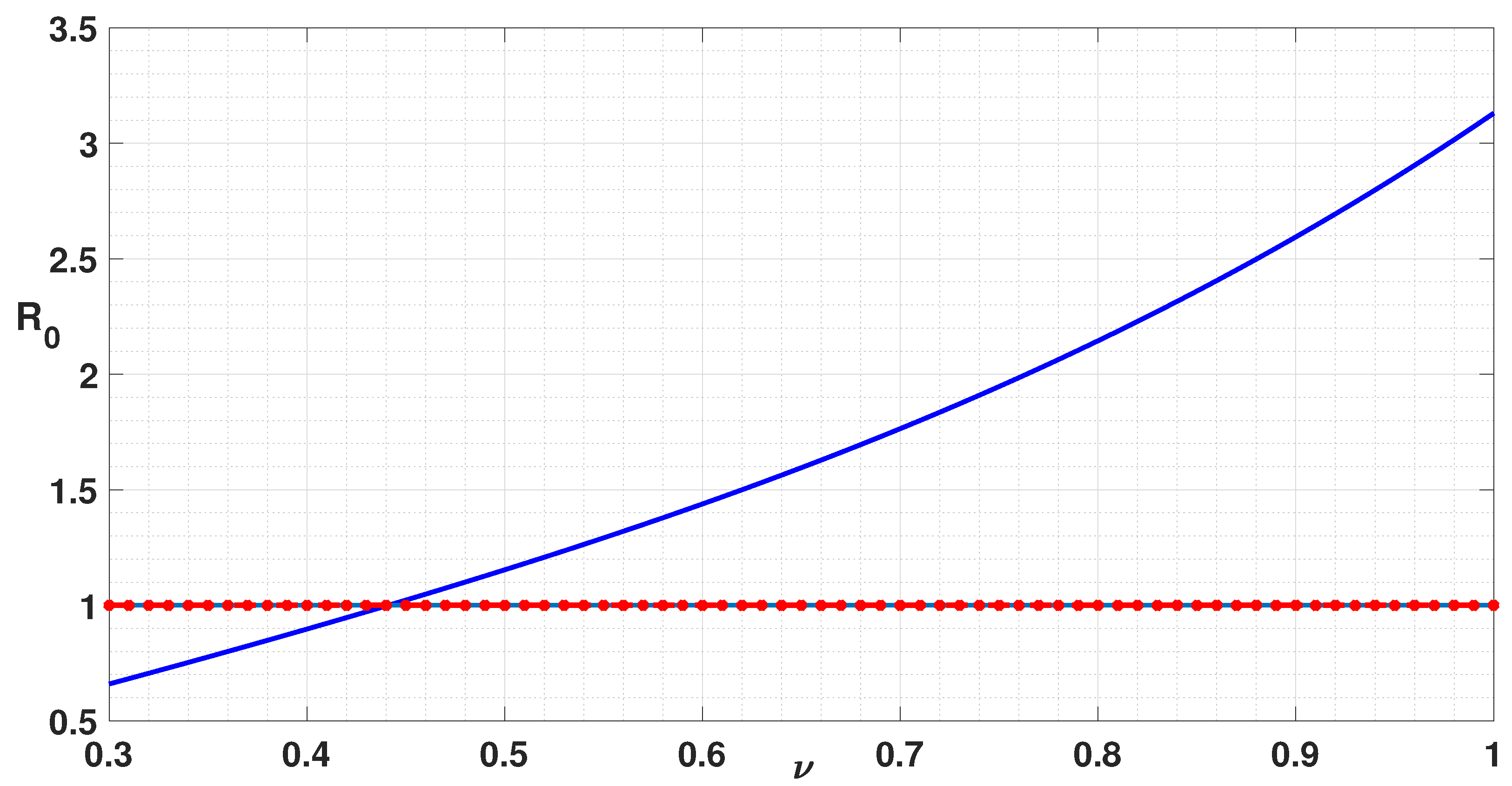
In this section, we present numerical simulations of the model using the parameter values listed in Table 2, which were estimated using real data from the measles outbreak in Nigeria [2]. From Equation (10), it is clear that the basic reproduction number varies according to the value of the fractional order $\nu$. Thus, for fractional orders $\nu \in 1,0.9,0.8,0.7,0.6$, the corresponding values of the basic reproduction number $R_0$ are, respectively, $3.13$, $2.60$, $2.15$, $1.76$, and $1.44$. From Figure 5, it is clear that $R_0$ is an increasing function of the fractional order $\nu$.

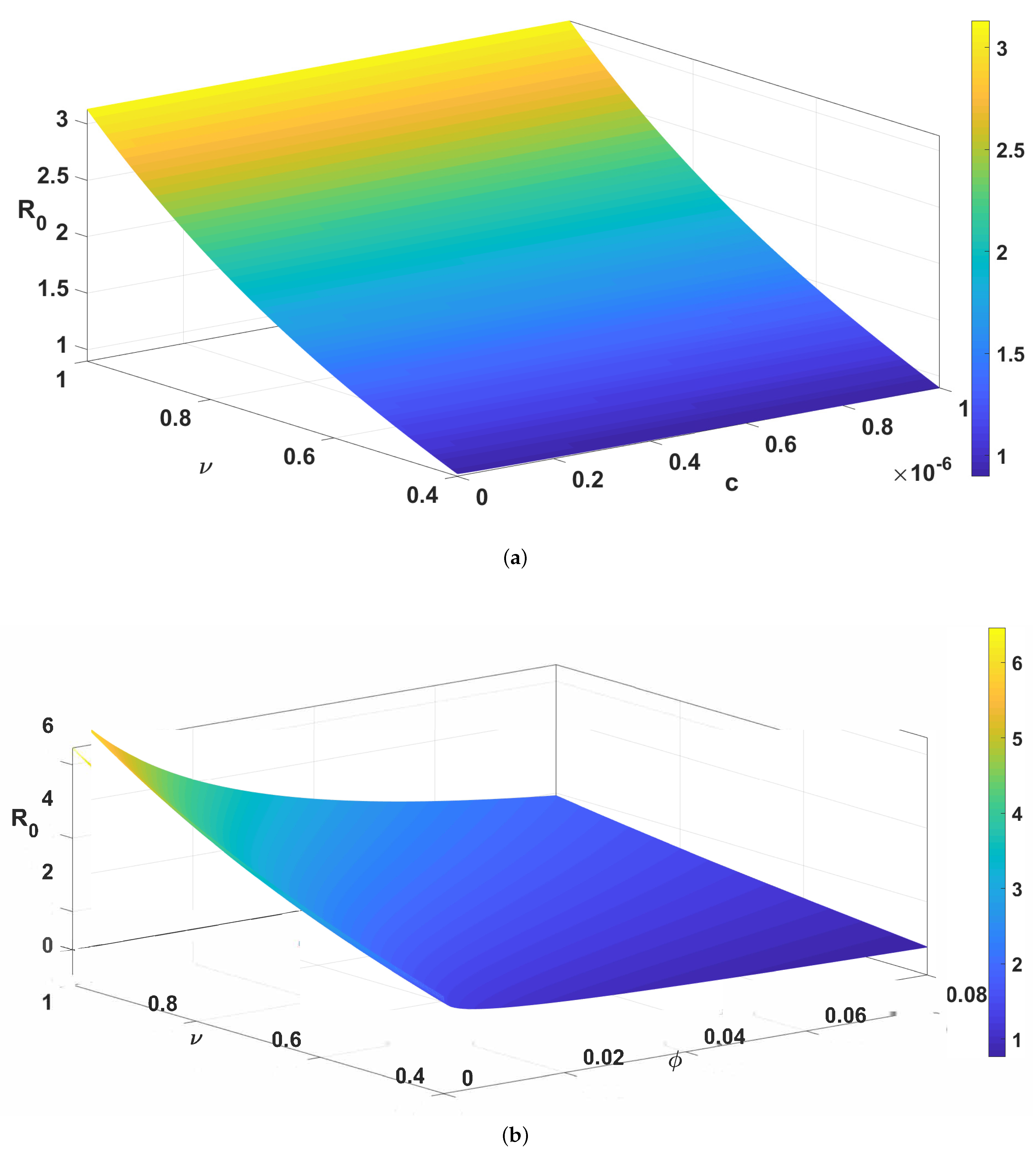
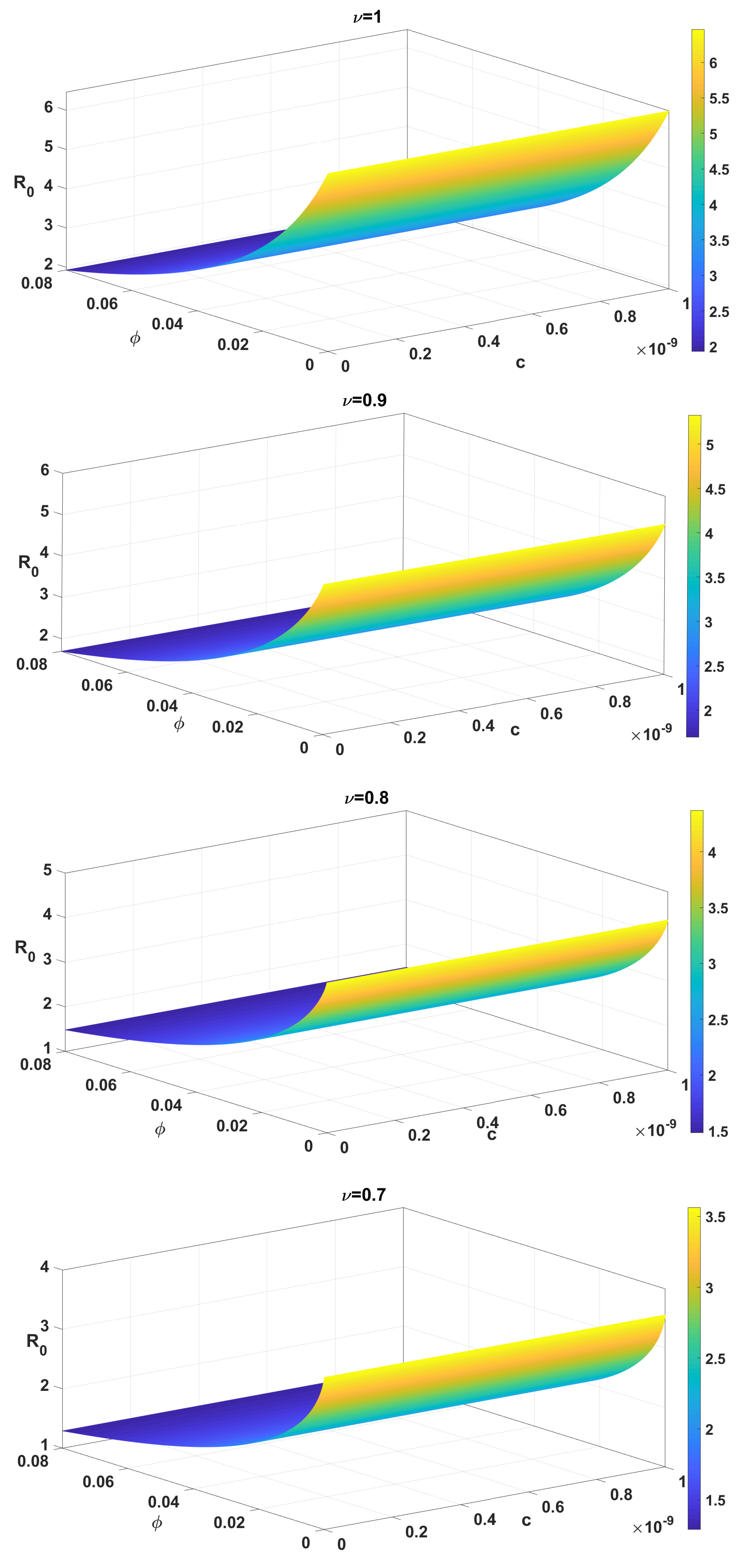
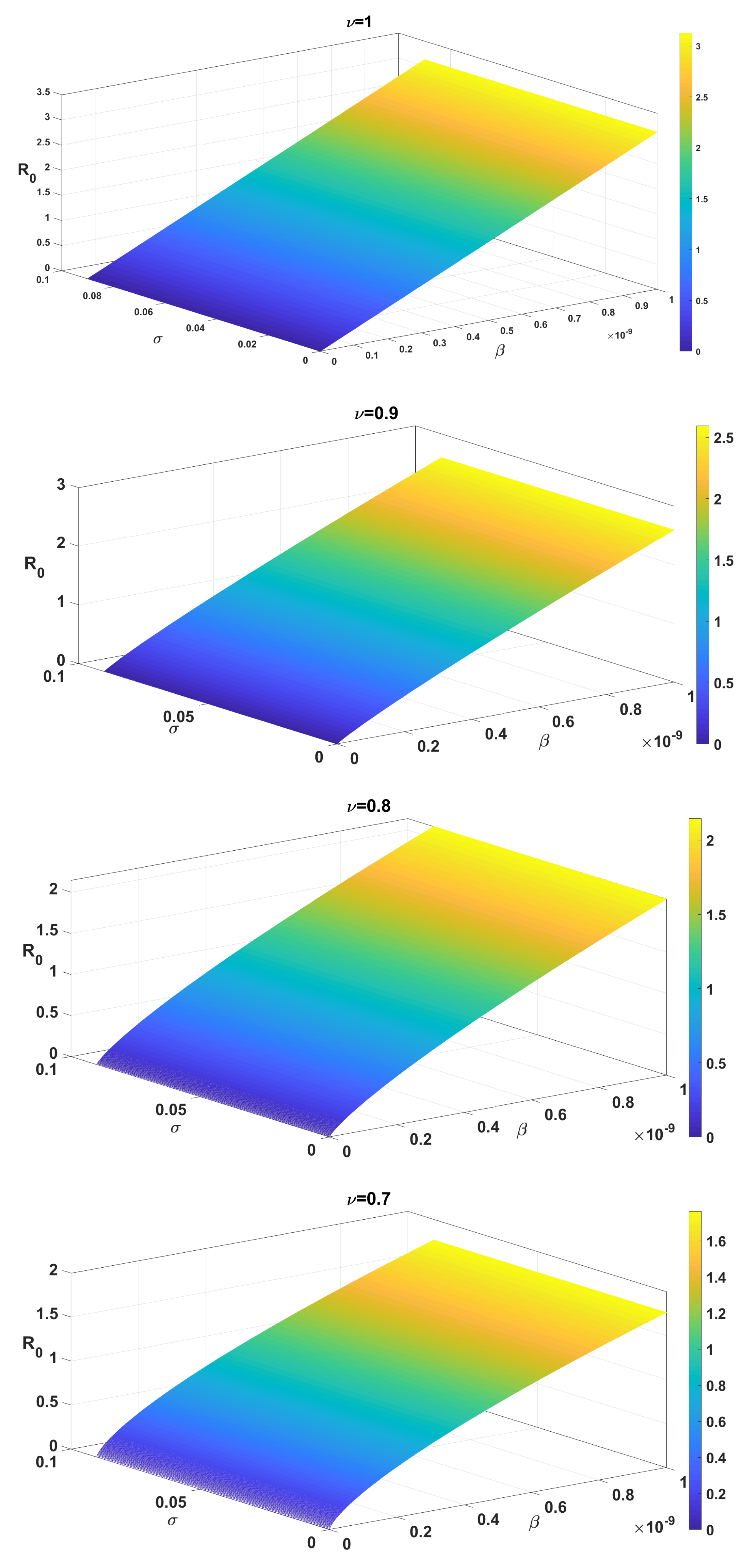
Figure 6a shows the combined effect of the fractional order and vaccination on the basic reproduction number, while Figure 6b shows the combined effect of the fractional order and hospitalization on the basic reproduction number. We see that $R_0$ decreases according to the increases in the vaccination rate c. Note that for $\nu =1$ and $c\in \left\{{10}^{-6},{10}^{-3},{10}^{-2},{10}^{-1}\right\}$, the basic reproduction number is $R_0\in \left\{3.13,2.45,0.83,0.11\right\}$, for $\nu =0.9$ and $c\in \left\{{10}^{-6},{10}^{-3},{10}^{-2},{10}^{-1}\right\}$, the basic reproduction number is $R_0\in \left\{2.60,1.99,0.76,0.13\right\}$, for $\nu =0.8$ and $c\in \left\{{10}^{-6},{10}^{-3},{10}^{-2},{10}^{-1}\right\}$, the basic reproduction number is $R_0\in \left\{2.15,1.61,0.69,0.15\right\}$. This proves that the measles epidemic can be controllable if the vaccination rate coverage is very high (indeed, from $c=0.01$, ${\mathcal{R}}_0$ is less than one). Moreover, effectively caring for the sick makes it possible to reduce the number of infected. Indeed, ${\mathcal{R}}_0$ decreases when the hospitalized rate $\varphi$ increases. Figure 7 combines mass vaccination with the efficient treatment in the basic reproduction number, while the combining effect of individual protection with effective healthcare is depicted in Figure 8. It is clear that when these two control strategies are at their high levels, the basic reproduction number is less than one, which implies the end of the epidemic.

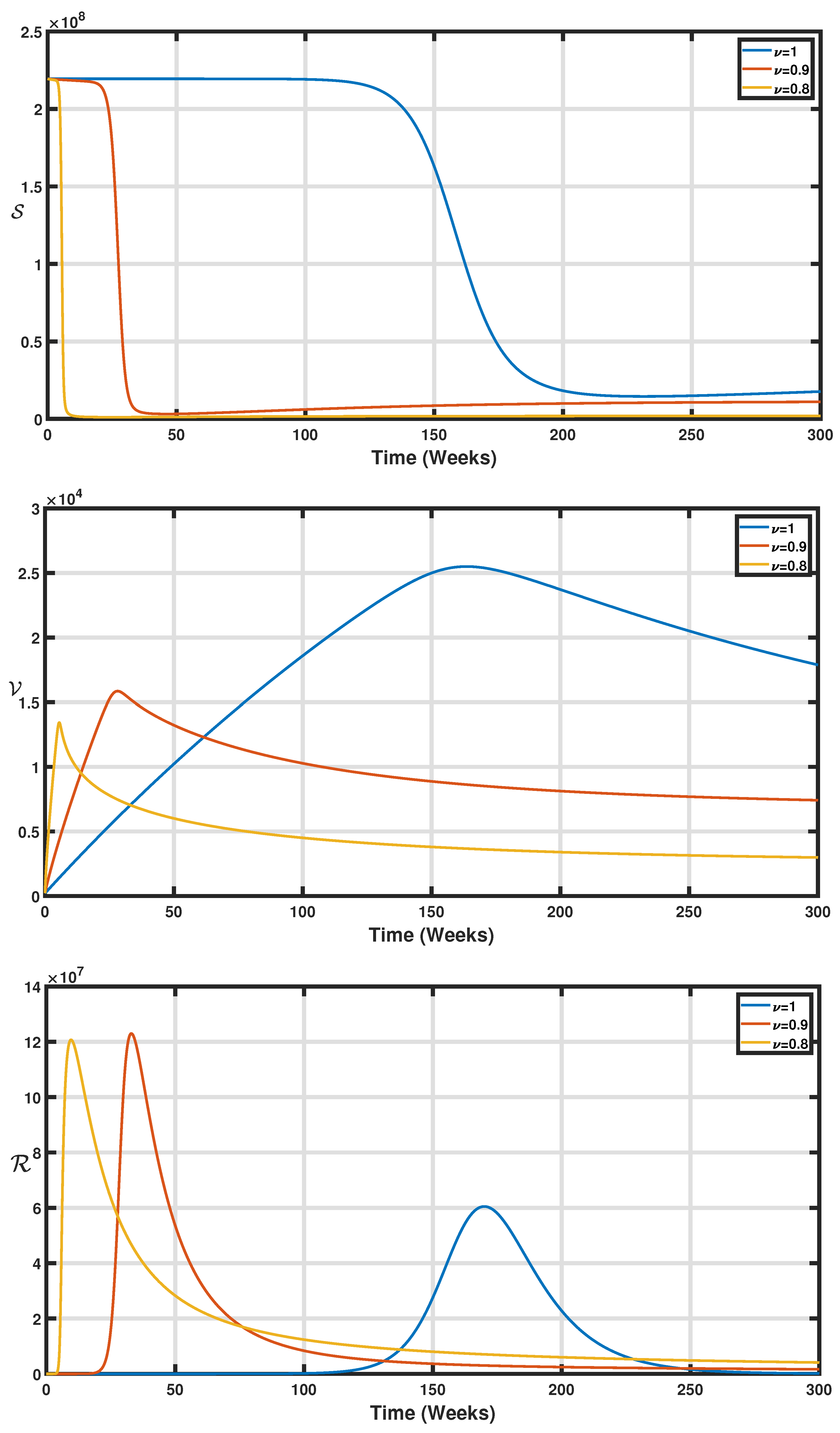
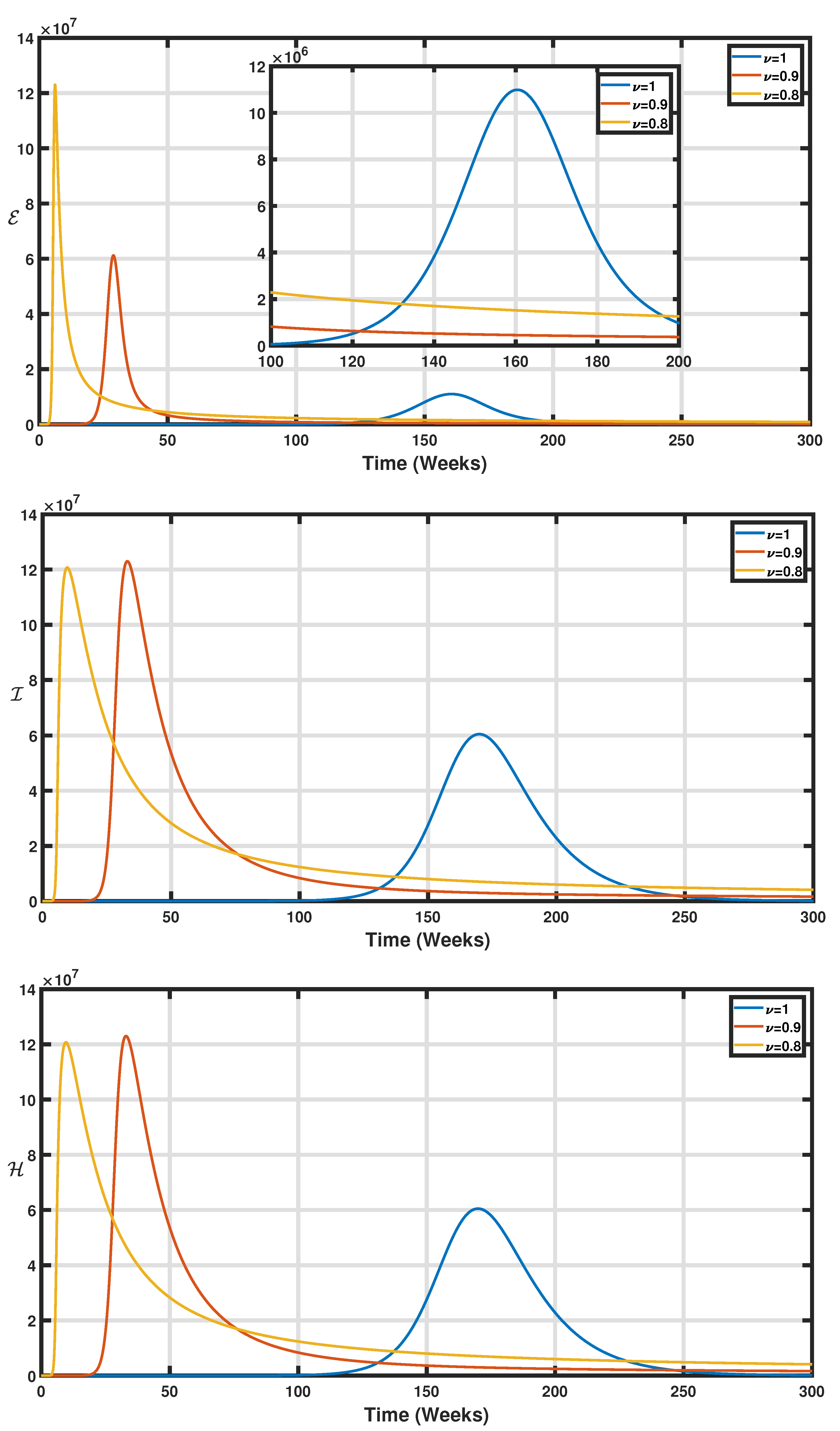
The effect of the fractional order on the dynamics of the measles model is depicted in Figure 9 and Figure 10. It is clear that susceptible (as well as vaccinated) individuals decrease according to the decrease of the fractional order $\nu$, while recovered individuals increase (Figure 9). The populations of all infected classes ($\mathcal{E}$, $\mathcal{I}$, and $\mathcal{H}$) increase when the fractional order decreases (Figure 10). Nevertheless, we can observe in Figure 10 that the epidemic ‘pick’ is backward-delayed according to the decrease of the fractional order $\nu$. For example, the total number of infected individuals in the latent stage E tended to its maximum value (11,000,000) at the 160th week after the beginning of the epidemic for $\nu =1$, while this time was backward-delayed to the 15th week.

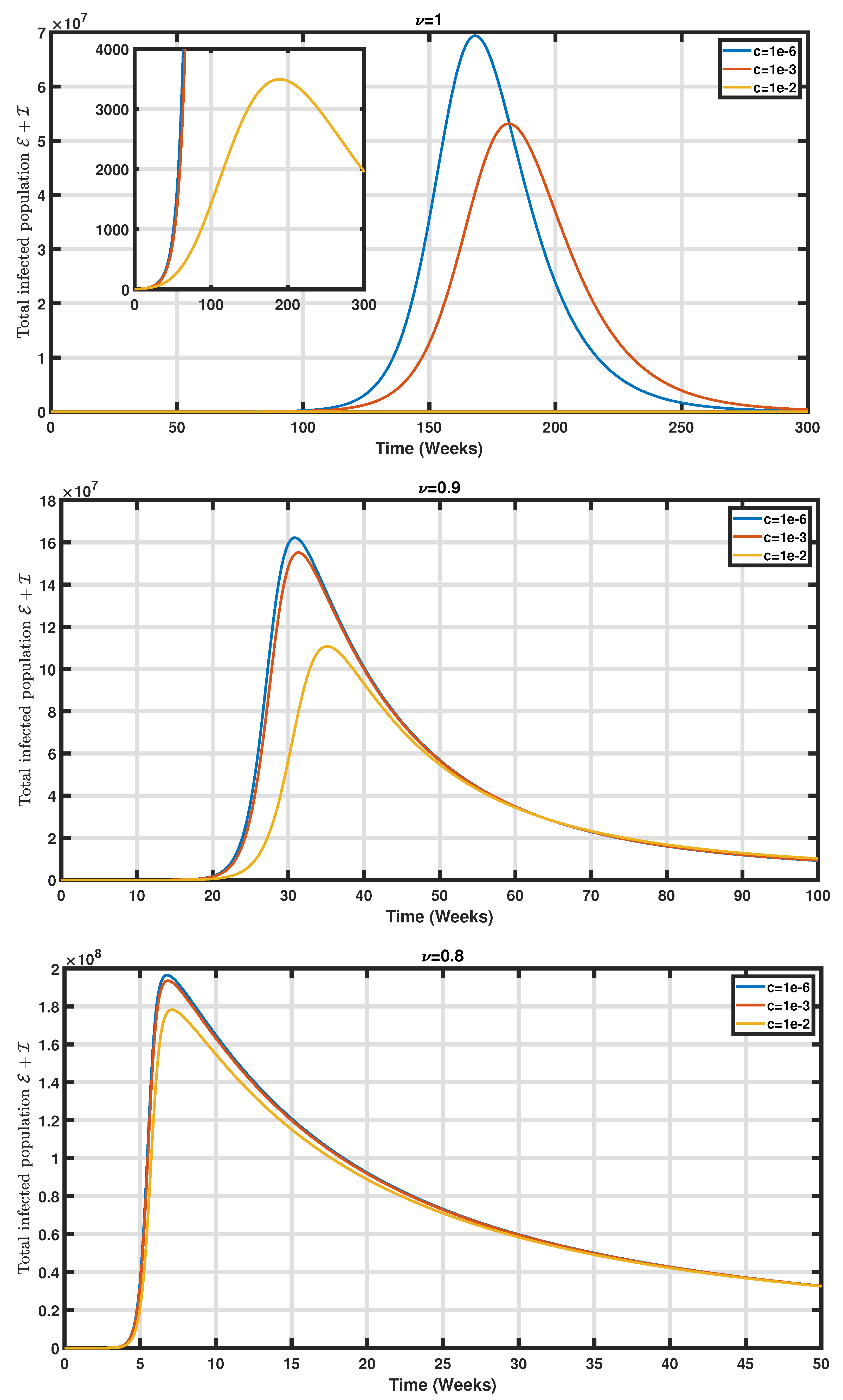
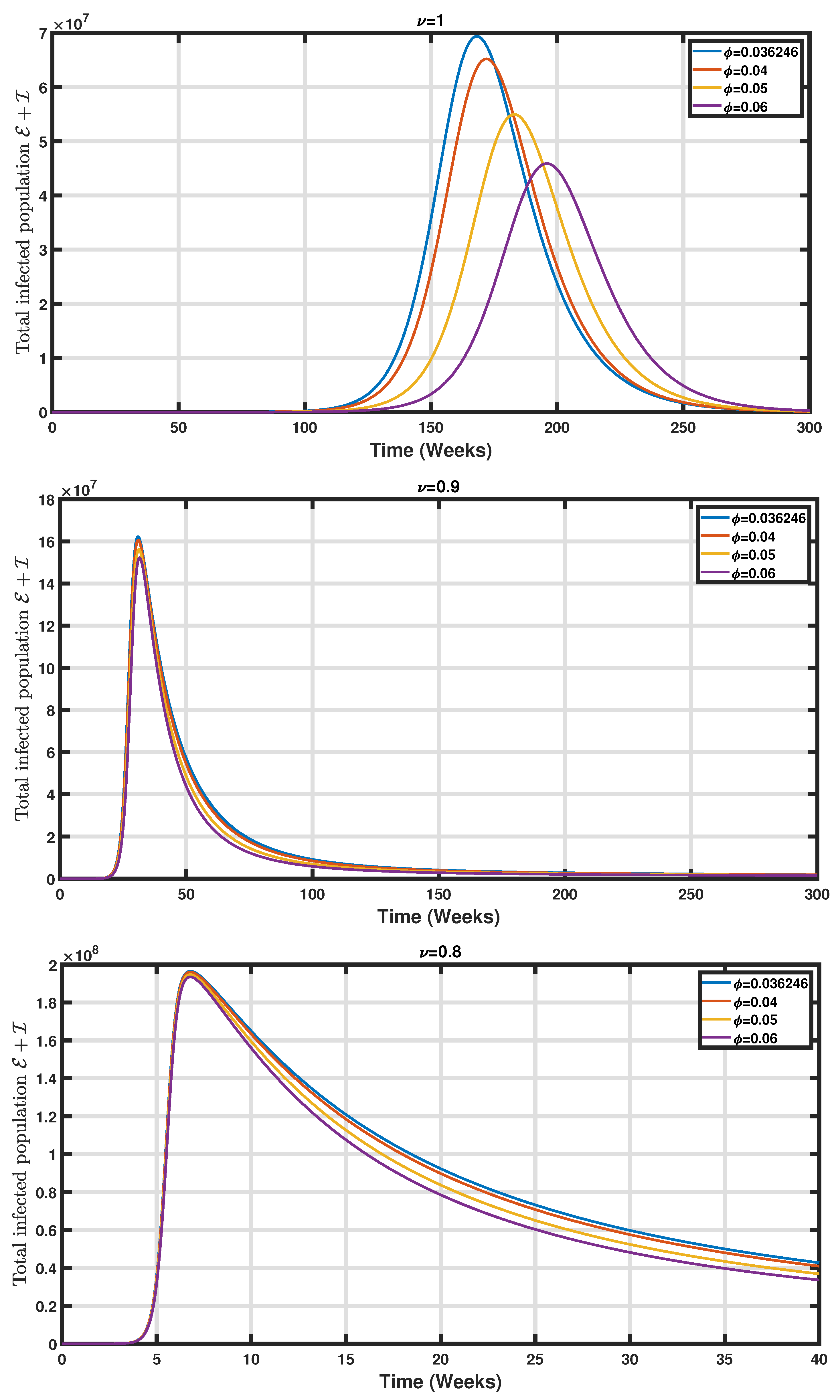
The effects of the two control measures, namely, vaccination and effective medical care, are depicted in Figure 11 and Figure 12. As in the case of the basic reproduction number, it is clear from Figure 11 that a high level of vaccination coverage can decrease the number of new cases of measles. Similarly, we see in Figure 12 that better care for patients (consisting of systematic hospitalization of new cases from the first symptoms of the disease) will allow for better control of the epidemic. Thus, the combination of these two control measures will help in the fight against the disease spread.

6. Conclusions and Perspectives

The main objective of this work was to compare the quantitative dynamics of an epidemic model of measles with the integer derivative and fractional derivative (in the sense of Caputo). Thus, we replaced the integer derivative with the Caputo derivative in an existing measles compartmental model, which took into account vaccinations and hospitalized individuals. We performed a global sensitivity analysis by computing the partial rank correlation coefficient between the model parameters, the basic reproduction number, and each state variable of the model. For the fractional model, we computed the basic reproduction number, which is a function of the model parameters and fractional-order parameter. We proved the local and global stability of the disease-free equilibrium as well as the local stability of the endemic equilibrium point. The existence, uniqueness of the solutions, and global stability of the fractional model were also conducted using the Ulam–Hyers stability method. Simulations via the Adams-type predictor–corrector iterative scheme, were conducted to validate our theoretical results and to see the impact of the variation of the fractional order on the disease dynamics. Indeed, the simulation results reveal that the model with the Caputo fractional derivative has a different quantitative behavior than the model with the integer derivative. This suggests that depending on the fractional order, we can forecast the number of total cases in a given interval of time.

It is important to note that some other aspects, such as limited medical resources, mass vaccination, and other fractional derivatives operator (Caputo–Fabrizio, Atangana–Baleanu, piecewise derivatives) can represent direct perspectives to this work. Moreover, there is evidence that the measles vaccine is flawed [63]. Thus, another future direction of this work would be to consider that some individuals who received the measles vaccine may be infected.

References

- Griffin, D.E. The immune response in measles: Virus control, clearance and protective immunity. Viruses 2016, 8, 282. [Google Scholar] [CrossRef] [PubMed] [Green Version]
- James Peter, O.; Ojo, M.M.; Viriyapong, R.; Abiodun Oguntolu, F. Mathematical model of measles transmission dynamics using real data from Nigeria. J. Differ. Equ. Appl. 2022, 1–18. [Google Scholar] [CrossRef]
- Roberts, M.; Tobias, M. Predicting and preventing measles epidemics in New Zealand: Application of a mathematical model. Epidemiol. Infect. 2000, 124, 279–287. [Google Scholar] [CrossRef] [PubMed]
- Subaiya, S.; Tabu, C.; N’ganga, J.; Awes, A.A.; Sergon, K.; Cosmas, L.; Styczynski, A.; Thuo, S.; Lebo, E.; Kaiser, R.; et al. Use of the revised World Health Organization cluster survey methodology to classify measles-rubella vaccination campaign coverage in 47 counties in Kenya, 2016. PLoS ONE 2018, 13, e0199786. [Google Scholar] [CrossRef] [Green Version]
- Nabi, K.N.; Abboubakar, H.; Kumar, P. Forecasting of COVID-19 pandemic: From integer derivatives to fractional derivatives. Chaos Solitons Fractals 2020, 141, 110283. [Google Scholar] [CrossRef]
- Inaba, H. Kermack and McKendrick revisited: The variable susceptibility model for infectious diseases. Jpn. J. Ind. Appl. Math. 2001, 18, 273–292. [Google Scholar] [CrossRef]
- Kermack, W.O.; McKendrick, A.G. Contributions to the mathematical theory of epidemics. II.—The problem of endemicity. Proc. R. Soc. Lond. Ser. Contain. Pap. Math. Phys. Character 1932, 138, 55–83. [Google Scholar]
- Raza, A.; Rafiq, M.; Baleanu, D.; Shoaib Arif, M.; Naveed, M.; Ashraf, K. Competitive numerical analysis for stochastic HIV/AIDS epidemic model in a two-sex population. IET Syst. Biol. 2019, 13, 305–315. [Google Scholar] [CrossRef] [PubMed]
- Sánchez, Y.G.; Sabir, Z.; Guirao, J.L. Design of a nonlinear SITR fractal model based on the dynamics of a novel coronavirus (COVID-19). Fractals 2020, 28, 2040026. [Google Scholar] [CrossRef]
- Shoaib, M.; Anwar, N.; Ahmad, I.; Naz, S.; Kiani, A.K.; Raja, M.A.Z. Intelligent networks knacks for numerical treatment of nonlinear multi-delays SVEIR epidemic systems with vaccination. Int. J. Mod. Phys. B 2022, 2250100. [Google Scholar] [CrossRef]
- Umar, M.; Sabir, Z.; Zahoor Raja, M.A.; Gupta, M.; Le, D.N.; Aly, A.A.; Guerrero-Sánchez, Y. Computational intelligent paradigms to solve the nonlinear SIR system for spreading infection and treatment using Levenberg–Marquardt backpropagation. Symmetry 2021, 13, 618. [Google Scholar] [CrossRef]
- Umar, M.; Kusen; Raja, M.A.Z.; Sabir, Z.; Al-Mdallal, Q. A computational framework to solve the nonlinear dengue fever SIR system. Comput. Methods Biomech. Biomed. Eng. 2022, 1–14. [Google Scholar] [CrossRef] [PubMed]
- Arsal, S.R.; Aldila, D.; Handari, B.D. Short review of mathematical model of measles. AIP Conf. Proc. 2020, 2264, 02003. [Google Scholar]
- Aldila, D.; Asrianti, D. A deterministic model of measles with imperfect vaccination and quarantine intervention. J. Phys. Conf. Ser. 2019, 1218, 012044. [Google Scholar] [CrossRef]
- Bashir, A.; Mushtaq, M.; Zafar, Z.U.A.; Rehan, K.; Muntazir, R.M.A. Comparison of fractional order techniques for measles dynamics. Adv. Differ. Equ. 2019, 2019, 334. [Google Scholar] [CrossRef]
- Berhe, H.W.; Makinde, O.D. Computational modelling and optimal control of measles epidemic in human population. Biosystems 2020, 190, 104102. [Google Scholar] [CrossRef] [PubMed]
- Memon, Z.; Qureshi, S.; Memon, B.R. Mathematical analysis for a new nonlinear measles epidemiological system using real incidence data from Pakistan. Eur. Phys. J. Plus 2020, 135, 378. [Google Scholar] [CrossRef]
- Momoh, A.; Ibrahim, M.; Uwanta, I.; Manga, S. Mathematical model for control of measles epidemiology. Int. J. Pure Appl. Math. 2013, 87, 707–718. [Google Scholar] [CrossRef] [Green Version]
- Mossong, J.; Muller, C.P. Modelling measles re-emergence as a result of waning of immunity in vaccinated populations. Vaccine 2003, 21, 4597–4603. [Google Scholar] [CrossRef]
- Obumneke, C.; Adamu, I.I.; Ado, S.T. Mathematical model for the dynamics of measles under the combined effect of vaccination and measles therapy. Int. J. Sci. Technol. 2017, 6, 862–874. [Google Scholar]
- Okyere-Siabouh, S.; Adetunde, I. Mathematical model for the study of measles in cape coast metropolis. Int. J. Mod. Biol. Med. 2013, 4, 110–133. [Google Scholar]
- Qureshi, S. Real life application of Caputo fractional derivative for measles epidemiological autonomous dynamical system. Chaos Solitons Fractals 2020, 134, 109744. [Google Scholar] [CrossRef]
- Center of Disease Control and Prevention. Global Measles Outbreaks. Available online: https://www.cdc.gov/globalhealth/measles/data/global-measles-outbreaks.html (accessed on 12 June 2022).
- Relief, D. The Global Measles Epidemic Isn’t (Just) About Measles. Available online: https://reliefweb.int/report/world/global-measles-epidemic-isn-t-just-about-measles (accessed on 21 April 2022).
- Sun, H.; Zhang, Y.; Baleanu, D.; Chen, W.; Chen, Y. A new collection of real world applications of fractional calculus in science and engineering. Commun. Nonlinear Sci. Numer. Simul. 2018, 64, 213–231. [Google Scholar] [CrossRef]
- Abboubakar, H.; Kom Regonne, R.; Sooppy Nisar, K. Fractional Dynamics of Typhoid Fever Transmission Models with Mass Vaccination Perspectives. Fractal Fract. 2021, 5, 149. [Google Scholar] [CrossRef]
- Neirameh, A. New fractional calculus and application to the fractional-order of extended biological population model. Bol. Soc. Parana. Matemática 2018, 36, 115–128. [Google Scholar] [CrossRef]
- He, J.H.; Ji, F.Y. Two-scale mathematics and fractional calculus for thermodynamics. Therm. Sci. 2019, 23, 2131–2133. [Google Scholar] [CrossRef]
- Tarasov, V.E. On history of mathematical economics: Application of fractional calculus. Mathematics 2019, 7, 509. [Google Scholar] [CrossRef] [Green Version]
- Caputo, M. Linear models of dissipation whose Q is almost frequency independent—II. Geophys. J. Int. 1967, 13, 529–539. [Google Scholar] [CrossRef]
- Derbazi, C.; Baitiche, Z.; Abdo, M.S.; Shah, K.; Abdalla, B.; Abdeljawad, T. Extremal Solutions of Generalized Caputo-Type Fractional-Order Boundary Value Problems Using Monotone Iterative Method. Fractal Fract. 2022, 6, 146. [Google Scholar] [CrossRef]
- Haidong, Q.; Arfan, M. Fractional model of smoking with relapse and harmonic mean type incidence rate under Caputo operator. J. Appl. Math. Comput. 2022, 1–18. [Google Scholar] [CrossRef]
- Jarad, F.; Abdeljawad, T.; Baleanu, D. On the generalized fractional derivatives and their Caputo modification. Int. Sci. Res. Publ. 2017. [Google Scholar] [CrossRef] [Green Version]
- Li, L.; Liu, J.G. A generalized definition of Caputo derivatives and its application to fractional ODEs. SIAM J. Math. Anal. 2018, 50, 2867–2900. [Google Scholar] [CrossRef] [Green Version]
- Odibat, Z.; Baleanu, D. Numerical simulation of initial value problems with generalized Caputo-type fractional derivatives. Appl. Numer. Math. 2020, 156, 94–105. [Google Scholar] [CrossRef]
- Xu, C.; Liao, M.; Li, P.; Guo, Y.; Liu, Z. Bifurcation properties for fractional order delayed BAM neural networks. Cogn. Comput. 2021, 13, 322–356. [Google Scholar] [CrossRef]
- Xu, C.; Zhang, W.; Aouiti, C.; Liu, Z.; Yao, L. Further analysis on dynamical properties of fractional-order bi-directional associative memory neural networks involving double delays. Math. Methods Appl. Sci. 2022. [Google Scholar] [CrossRef]
- Xu, C.; Liao, M.; Li, P.; Yuan, S. Impact of leakage delay on bifurcation in fractional-order complex-valued neural networks. Chaos Solitons Fractals 2021, 142, 110535. [Google Scholar] [CrossRef]
- Caputo, M.; Fabrizio, M. A new definition of fractional derivative without singular kernel. Progr. Fract. Differ. Appl. 2015, 1, 73–85. [Google Scholar]
- Atangana, A.; Baleanu, D. New fractional derivatives with non-local and non-singular kernel: Theory and Application to Heat Transfer Model. arXiv 2016, arXiv:1602.03408. [Google Scholar]
- Liu, X.; Arfan, M.; Ur Rahman, M.; Fatima, B. Analysis of SIQR type mathematical model under Atangana-Baleanu fractional differential operator. Comput. Methods Biomech. Biomed. Eng. 2022, 3, 1–15. [Google Scholar] [CrossRef] [PubMed]
- Zifan, A.; Saberi, S.; Moradi, M.H.; Towhidkhah, F. Automated ECG segmentation using piecewise derivative dynamic time warping. Int. J. Biol. Med. Sci. 2006, 1. Available online: https://www.researchgate.net/publication/228734344_Automated_ECG_Segmentation_Using_Piecewise_Derivative_Dynamic_Time_Warping (accessed on 26 June 2022).
- Abboubakar, H.; Kumar, P.; Rangaig, N.A.; Kumar, S. A malaria model with Caputo–Fabrizio and Atangana–Baleanu derivatives. Int. J. Model. Simulation, Sci. Comput. 2021, 12, 2150013. [Google Scholar] [CrossRef]
- Atangana, A. Mathematical model of survival of fractional calculus, critics and their impact: How singular is our world? Adv. Differ. Equ. 2021, 2021, 403. [Google Scholar] [CrossRef]
- Abdulazeez, S.T.; Modanli, M. Solutions of fractional order pseudo-hyperbolic telegraph partial differential equations using finite difference method. Alex. Eng. J. 2022, 61, 12443–12451. [Google Scholar] [CrossRef]
- Farman, M.; Saleem, M.U.; Ahmad, A.; Ahmad, M. Analysis and numerical solution of SEIR epidemic model of measles with non-integer time fractional derivatives by using Laplace Adomian Decomposition Method. Ain Shams Eng. J. 2018, 9, 3391–3397. [Google Scholar] [CrossRef]
- Ogunmiloro, O.M.; Idowu, A.S.; Ogunlade, T.O.; Akindutire, R.O. On the Mathematical Modeling of Measles Disease Dynamics with Encephalitis and Relapse Under the Atangana–Baleanu–Caputo Fractional Operator and Real Measles Data of Nigeria. Int. J. Appl. Comput. Math. 2021, 7, 185. [Google Scholar] [CrossRef]
- Qureshi, S. Monotonically decreasing behavior of measles epidemic well captured by Atangana–Baleanu–Caputo fractional operator under real measles data of Pakistan. Chaos Solitons Fractals 2020, 131, 109478. [Google Scholar] [CrossRef]
- Qureshi, S.; Jan, R. Modeling of measles epidemic with optimized fractional order under Caputo differential operator. Chaos Solitons Fractals 2021, 145, 110766. [Google Scholar] [CrossRef]
- Diethelm, K. An algorithm for the numerical solution of differential equations of fractional order. Electron. Trans. Numer. Anal 1997, 5, 1–6. [Google Scholar]
- Diethelm, K.; Ford, N.J.; Freed, A.D. A predictor-corrector approach for the numerical solution of fractional differential equations. Nonlinear Dyn. 2002, 29, 3–22. [Google Scholar] [CrossRef]
- Marino, S.; Hogue, I.B.; Ray, C.J.; Kirschner, D.E. A methodology for performing global uncertainty and sensitivity analysis in systems biology. J. Theor. Biol. 2008, 254, 178–196. [Google Scholar] [CrossRef] [Green Version]
- Wu, J.; Dhingra, R.; Gambhir, M.; Remais, J.V. Sensitivity analysis of infectious disease models: Methods, advances and their application. J. R. Soc. Interface 2013, 10, 20121018. [Google Scholar] [CrossRef] [PubMed] [Green Version]
- Stein, M. Large sample properties of simulations using Latin hypercube sampling. Technometrics 1987, 29, 143–151. [Google Scholar] [CrossRef]
- Bozkurt, F.; Yousef, A.; Abdeljawad, T.; Kalinli, A.; Al Mdallal, Q. A fractional-order model of COVID-19 considering the fear effect of the media and social networks on the community. Chaos Solitons Fractals 2021, 152, 111403. [Google Scholar] [CrossRef] [PubMed]
- Podlubny, I. Fractional Differential Equations: An Introduction to Fractional Derivatives, Fractional Differential Equations, to Methods of Their Solution and Some of Their Applications; Elsevier: Amsterdam, The Netherlands, 1998. [Google Scholar]
- Diethelm, K. The Analysis of Fractional Differential Equations: An Application-Oriented Exposition Using Differential Operators of Caputo Type; Springer: Berlin/Heidelberg, Germany, 2010. [Google Scholar]
- Lin, W. Global existence theory and chaos control of fractional differential equations. J. Math. Anal. Appl. 2007, 332, 709–726. [Google Scholar] [CrossRef] [Green Version]
- Akindeinde, S.O.; Okyere, E.; Adewumi, A.O.; Lebelo, R.S.; Fabelurin, O.O.; Moore, S.E. Caputo fractional-order SEIRP model for COVID-19 Pandemic. Alex. Eng. J. 2022, 61, 829–845. [Google Scholar] [CrossRef]
- Jung, S.M. Hyers-Ulam-Rassias Stability of Functional Equations in Nonlinear Analysis; Springer: Berlin/Heidelberg, Germany, 2011; Volume 48. [Google Scholar]
- Li, C.; Zeng, F. The finite difference methods for fractional ordinary differential equations. Numer. Funct. Anal. Optim. 2013, 34, 149–179. [Google Scholar] [CrossRef]
- Kumar, P.; Rangaig, N.A.; Abboubakar, H.; Kumar, A.; Manickam, A. Prediction studies of the epidemic peak of coronavirus disease in Japan: From Caputo derivatives to Atangana–Baleanu derivatives. Int. J. Model. Simul. Sci. Comput. 2022, 13, 2250012. [Google Scholar] [CrossRef]
- van Boven, M.; Kretzschmar, M.; Wallinga, J.; O’Neill, P.D.; Wichmann, O.; Hahné, S. Estimation of measles vaccine efficacy and critical vaccination coverage in a highly vaccinated population. J. R. Soc. Interface 2010, 7, 1537–1544. [Google Scholar] [CrossRef]
Figure 2.
Partial rank correlation coefficients between the basic reproduction number and model parameters.
Figure 3.
Partial rank correlation coefficients between uninfected state variables of the model and model parameters.
Figure 4.
Partial rank correlation coefficients between infected state variables of the model and model parameters.
Figure 5.
The basic reproduction number versus the fractional order . All other parameter values are listed in Table 2.
Figure 6.
The basic reproduction number versus (a) the vaccination rate c and the fractional order ; (b) the hospitalized rate and the fractional order .
Figure 7.
The basic reproduction number versus the vaccination rate c and the hospitalization rate .
Figure 8.
The basic reproduction number versus the transmission rate and the recovered rate .
Figure 9.
The time series of non-infected state variables of the model Equation (9) with the parameter values listed in Table 2 and different values for the fractional order derivatives .
Figure 10.
The time series of infected state variables of the model Equation (9) with the parameter values listed in Table 2 and different values for the fractional order derivatives .
Figure 11.
The time series of the total infected population with the parameter values listed in Table 2, except the vaccination rate c and the fractional order derivative , which vary.
Figure 12.
The time series of the total infected population with the parameter values listed in Table 2, except the hospitalized rate and the fractional order derivative , which vary.