The SLI-SC Mathematical Model of African Swine Fever Transmission among Swine Farms: The Effect of Contaminated Human Vector

Abstract

In this paper, a mathematical model for African swine fever is modified by considering the swine farm with the contaminated human vector that is able to infect and spread the disease among swine farms. In the developed model, we have divided the swine farm density into three related groups, namely the susceptible swine farm compartment, latent swine farm compartment, and infectious swine farm compartment. On the other hand, the human vector population density has been separated into two classes, namely the susceptible human vector compartment and the infectious human vector compartment. After that, we use this model and a quarantine strategy to analyze the spread of the infection. In addition, the basic reproduction number $R_0$ is determined by using the next-generation matrix, which can analyze the stability of the model. Finally, the numerical simulations of the proposed model are illustrated to confirm the results from theorems. The results showed that the transmission coefficient values per unit of time per individual between the human vector and the swine farm resulted in the spread of African swine fever.

1. Introduction

African swine fever (ASF) is a devastating transboundary animal disease in swine (domestic pig) that has been spreading over many regions of the world for decades [1]. The etiological agent of ASF is the only member in the genus Asfivirus, family Asfarviridae, a double-stranded DNA virus called African swine fever virus (ASFV) [2]. Although ASF cannot be transmitted from swine to humans [3], ASFV can transmit between swine on the same farm by direct contact. At the same time, the spread between farms is caused not only by ticks [4] or feeding a swine with infectious product [5] but also by a vector such as contaminated humans [6,7]. In addition, since ASFV has an extremely high potential to survive in an infected swine or a pork product for a long time, a few infected swine farms can easily lead to a transboundary outbreak. Moreover, at present, there is no effective vaccine or treatment available for this disease [2,8]. ASF can affect an infected swine with up to 100% chance of mortality [9,10]. Since pork plays a crucial role as a human food source in many countries, the endemic of ASF may result in severe economic loss. As a consequence, the measure that may be used to prevent the endemic is to exterminate all swine on the farm that found the disease.

In order to overcome this disease, a vaccine for ASF may be the best solution that we can have to fight the virus. However, in the situation that there is no vaccine available yet [11,12], the understanding of the endemic behavior and situation is an essential factor in controlling the severity of the disease. Therefore, research in the medical science field may be the best way that leads to the invention of the vaccine. On the other hand, to understand disease behavior, mathematical modeling is one of the powerful techniques that have been widely carried out to provide the information and accurate prediction of a lot of disease phenomena [13,14,15].

Traditionally, mathematical models of the ASF endemic have been studied by considering individual swine [15,16,17,18]. Barongo et al. [16] presented a SEICD model where S denotes a susceptible state, E denotes the state that is infected but not yet infectious, I denotes the infectious state, C denotes the carrier state, and D denotes the dead state. The model emphasized the need for biosecurity and vaccines to overcome the disease. Halasa et al. [19] studied the model for ASF transmission that separates swine into five classes: susceptible, latent, subclinical, and recovered. The result shows the significance of subclinical swine’s infectiousness and the dead swine’s residues in the spread of ASF. Ma et al. [20] investigated the transmission of ASF in Vietnam using a dynamic SIR model. The result shows that an effective vaccine (if it exists) would play a crucial role in preventing the ASF endemic. However, biosecurity can still be an essential tool to control the spread of the disease on a small-scale farm. However, swine are reared on a dense farm containing more than 100 individuals. Hence, ASF infection on all swine on a farm occurs almost at the same time. In this regard, it is a suitable choice to study disease by considering the spread among individual farms in a study of individual swine.

The ASF model is constructed based on a system of ordinary differential equations describing the rate of change for involving variables. By linearlizing the system, the model can be rewritten in the form of matrix equation $X^{\prime }=AX$. Suppose that the solution $X\left(t\right)$ is in the form $X=C{e}^{\lambda t}$, the behavior of the solution can be analyzed using the well-known method known as Eigenvector-Eigenvalue problem.

According to the argument mentioned above, to study endemic ASF, we develop a mathematical model by considering the swine population in the model as individual farms. The SLI-SC (Susceptible-Latent-Infectious-Susceptible-Contaminated) model is presented in Section 2. The analysis of the mathematical model is shown in Section 3. Then, Section 4 discusses the numerical examples of the proposed model. Finally, a conclusion is presented Section 5.

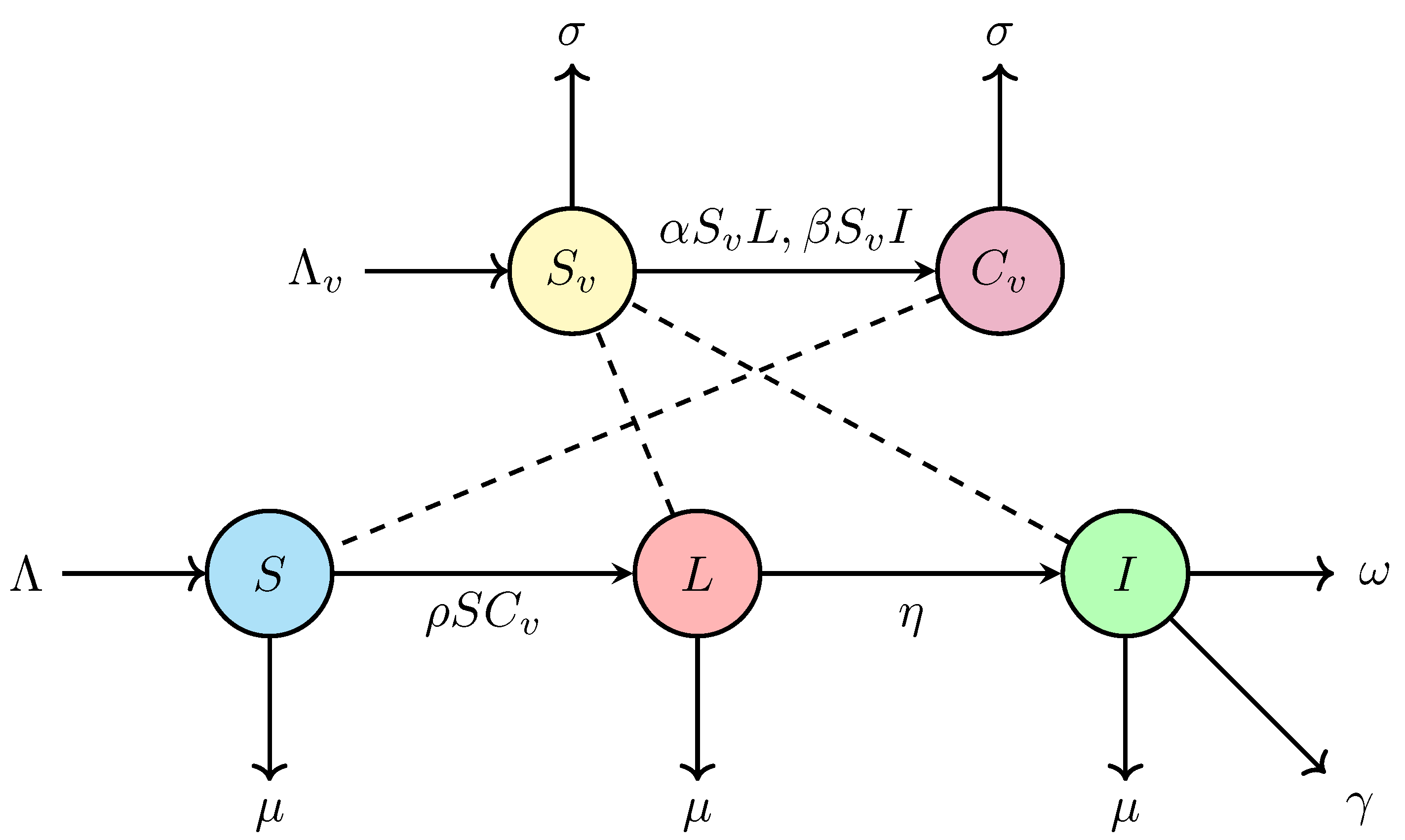
2. Mathematical Modeling

In this study, an individual in the population is considered an individual swine farm. Based on the SIR and other involving models [21,22,23,24,25], we divided the population into three classes including susceptible class $\left(S\right)$, latent class $\left(L\right)$, and infectious class $\left(I\right)$. Since the transmission of ASF disease between swine farms is a consequence of the infectious vector, the susceptible class $\left(S_v\right)$ and contaminated class $\left(C_v\right)$ of the vector are taken into account. Therefore, we can describe the behavior of the ASF endemic by using the SLI-SC model as follows:

$$\begin{array}{cc}\hfill \frac{dS}{dt}& =\Lambda -\rho S{C}_v-\mu S,\hfill \\ \hfill \frac{dL}{dt}& =\rho S{C}_v-\eta L-\mu L,\hfill \\ \hfill \frac{dI}{dt}& =\eta L-(\mu +\gamma +\omega )I,\hfill \\ \hfill \frac{d{S}_v}{dt}& ={\Lambda }_v-\alpha S_{v}L-\beta S_{v}I-\sigma S_v,\hfill \\ \hfill \frac{d{C}_v}{dt}& =\alpha S_{v}L+\beta S_{v}I-\sigma C_v,\hfill \end{array}$$

(1)

where $\Lambda$ denotes the recruited rate, $\rho$ denotes the transmission coefficient per unit of time per individual in the susceptible class S contact with the contaminated class $C_v$, $\eta$ denotes the transition rate per unit of time from the latent class L to the infectious class I, $\alpha$ and $\beta$ denote the transmission coefficient per unit of time per individual in the susceptible class $S_v$ contact with the latent class L and the infectious class I, respectively, $\mu$, $\gamma$, $\omega$ denote the mortality rate of swine per farm by nature, disease, government control policies for ASF, respectively, and ${\Lambda }_v$ and $\sigma$ denote the recruited and mortality rate of the vector.

A flowchart of the SLI-SC model of swine and human vector described by the system (1) is shown in Figure 1.

3. Analysis of the Model

In this section, we investigate the existence of the solution of the proposed model (1), the positivity of the solution, and the equilibria of the model. Then, the basic reproduction number of the model is obtained. We also propose theorems representing the sufficient conditions for local and global stability of both disease-free equilibrium and endemic equilibrium.

3.1. Existence of the Solution

Lemma 1

(Derrick and Groosman theorem [26]). Let Ω denote the region

$$|t-t_0|\le a,||u-u_0\left|\right|\le 1,u=(u_1,u_2,\dots ,u_n),u_0=(u_{10},u_{20},\dots ,u_{n0}),$$

and suppose that $f(t,u)$ satisfies the Lipchitz condition

$$\left|\right|f(t,u_1)-f(t,u_2)\left|\right|\le k\left|\right|u_1-u_2\left|\right|$$

whenever the pairs $(t,u_1)$ and $(t,u_2)$ belong to Ω where k is a positive constant. Then, there is a constant $a\ge 0$ such that there exists a unique continuous vector solution of $u\left(t\right)$ of the system in the interval $t-t_0\le a$.

It is important to note that the condition is satisfied by the requirement that $\partial f_i/\partial u_j\mathrm{for}i,$$j=1,2,3,\dots$ are continuous and bounded in Ω.

Theorem 1.

The solution of the model (1) with the initial conditions $S\left(0\right)\ge 0,L\left(0\right)\ge 0,I\left(0\right)\ge 0,$$S_v\left(0\right)\ge 0,C_v\left(0\right)\ge 0$ exists and is unique in ${\mathbb{R}}_{+}^5$ for all $t\ge 0.$

Proof. 

The right-hand sides of the system (1) can be expressed as follows:

$$\begin{array}{cc}\hfill f_1& =\Lambda -\rho S{C}_v-\mu S,\hfill \\ \hfill f_2& =\rho S{C}_v-\eta L-\mu L,\hfill \\ \hfill f_3& =\eta L-(\mu +\gamma +\omega )I,\hfill \\ \hfill f_4& ={\Lambda }_v-\alpha S_{v}L-\beta S_{v}I-\sigma S_v,\hfill \\ \hfill f_5& =\alpha S_{v}L+\beta S_{v}I-\sigma C_v.\hfill \end{array}$$

It is easy to obtain that $\partial f_i/\partial u_i$ are continuous and ${\displaystyle \left|\partial f_i/\partial u_i\right|<\infty }$ for $i,j=1,2,\cdots ,5$, where $u_1=S,u_2=L,u_3=I,u4=S_v,$ and $u_5=C_v$. By Lemma 1, the system (1) has a unique solution. □

3.2. Positivity of the Solution

Theorem 2.

The solution of the system (1) with the initial conditions $S\left(0\right)\ge 0,L\left(0\right)\ge 0,$$I\left(0\right)\ge 0,S_v\left(0\right)\ge 0,C_v\left(0\right)\ge 0$ is positive in ${\mathbb{R}}^5$ for all $t\ge 0$.

Proof. 

Positivity of $S\left(t\right)$: Suppose there exists $t_0$ such that $dS\left(t_0\right)/dt<0$ and $S\left(t_0\right)=0$. Considering the first equation of system (1), we have $dS/dt=\Lambda -\rho S{C}_v-\mu S$. When $t=t_0$, it follows that $S\left(t_0\right)=0$ by assumption. Then, $dS\left(t_0\right)/dt=\Lambda >0$. This contradicts the assumption that $dS\left(t_0\right)/dt<0$. By contradiction, $S\left(t\right)\ge 0$ for all $t\ge 0.$

Positivity of $S_v\left(t\right)$: Suppose there exists $t_0$ such that $d{S}_v\left(t_0\right)/dt<0$ and $S_v\left(t_0\right)=0$. Considering the fourth equation of system (1), we have $d{S}_v/dt={\Lambda }_v-\alpha S_{v}L-\beta S_{v}I-\sigma S_v$. When $t=t_0$, it follows that $S_v\left(t_0\right)=0$ by assumption. Then, $d{S}_v\left(t_0\right)/dt={\Lambda }_v>0$. This contradicts the assumption that $d{S}_v\left(t_0\right)/dt<0$. By contradiction, $S_v\left(t\right)\ge 0$ for all $t\ge 0.$

Positivity of $C_v\left(t\right)$: Suppose there exists $t_0=min\left\{\tau \right\}$ such that $d{C}_v\left(\tau \right)/dt<0$ and $C_v\left(\tau \right)=0.$ Thus, $C_v\left(t\right)>0$ for all $0<t<t_0.$ Considering the second term of system (1), $dL/dt\ge -\eta L-\mu L$ for $t\in (0,t_0).$ After applying integration, the solution can be written as $L\left(t\right)\ge L\left(0\right)\exp (-(\eta +\mu \left)t\right)>0$ for $t\in (0,t_0).$ By continuity, $L\left(t_0\right)>0.$ Similarly, $I\left(t\right)\ge I\left(0\right)\exp (-(\mu +\gamma +\omega \left)t\right)>0$ for $t\in (0,t_0)$ and $I\left(t_0\right)>0.$ The slope of $C_v$ at $t_0$ are defined by $d{C}_v\left(t_0\right)/dt=\alpha S_v\left(t_0\right)L\left(t_0\right)+\beta S_v\left(t_0\right)I\left(t_0\right)-\sigma C_v\left(t_0\right)\ge 0$. This contradicts the assumption that $d{C}_v\left(t_0\right)/dt<0$. By contradiction, $C_v\left(t\right)\ge 0$ for all $t\ge 0.$

Positivity of $L\left(t\right)$: Suppose there exists $t_0$ such that $dL\left(t_0\right)/dt<0$ and $L\left(t_0\right)=0$. Considering the second equation of system (1), we have $dL/dt=\rho S{C}_v-\eta L-\mu L$. When $t=t_0$, it follows that $L\left(t_0\right)=0$ by assumption. Then $dL\left(t_0\right)/dt=\rho S\left(t_0\right)C_v\left(t_0\right)\ge 0$. This contradicts the assumption that $dL\left(t_0\right)/dt<0$. By contradiction, $L\left(t\right)\ge 0$ for all $t\ge 0.$

Positivity of $I\left(t\right)$: Suppose there exists $t_0$ such that $dI\left(t_0\right)/dt<0$ and $I\left(t_0\right)=0$. Considering the third equation of system (1), we have $dI/dt=\eta L-(\mu +\gamma +\omega )I$. When $t=t_0$, it follows that $I\left(t_0\right)=0$ by assumption. Then $dI\left(t_0\right)/dt=\eta L\left(t_0\right)\ge 0$. This contradicts the assumption that $dI\left(t_0\right)/dt<0$. By contradiction, $I\left(t\right)\ge 0$ for all $t\ge 0.$

Therefore, the solution of system (1) is a positive quantity in ${\mathbb{R}}^5$ for all $t\ge 0$. □

3.3. Invariant Region

Let $N\left(t\right)$ and $N_v\left(t\right)$ are the total number of swine farm and the total human vector population at time t, respectively. It follows that

$$\begin{array}{cc}\hfill \frac{dN}{dt}& =\frac{dS}{dt}+\frac{dL}{dt}+\frac{dI}{dt}\hfill \\ \hfill & =\Lambda -\mu N-(\gamma +\omega )I.\hfill \end{array}$$

Then,

$$\underset{supt\to \infty }{lim}N\le \frac{\Lambda }{\mu }.$$

Similarly,

$$\begin{array}{cc}\hfill \frac{d{N}_v}{dt}& =\frac{d{S}_v}{dt}+\frac{d{C}_v}{dt}\hfill \\ \hfill & ={\Lambda }_v-\sigma N_v.\hfill \end{array}$$

Then, we get

$$\underset{supt\to \infty }{lim}{N}_v\le \frac{{\Lambda }_v}{\sigma }.$$

Therefore, the possible region for the system (1) is

$$\Omega =\left\{(S,L,I,S_v,C_v)\in {\mathbb{R}}^5:S\ge 0,L\ge 0,I\ge 0,S_v\ge 0,C_v\ge 0,N+N_v\le \frac{\Lambda }{\mu }+\frac{{\Lambda }_v}{\sigma }\right\}.$$

3.4. Equilibria

In this section, we derive equilibrium of the system (1) by equating all equations in the system (1) to zero. We obtain two equilibrium points as follows:

(i)

The disease-free equilibrium (DFE)

$$E^0=(S^0,L^0,I^0,S_v^0,C_v^0)=\left(\frac{\Lambda }{\mu },0,0,\frac{{\Lambda }_v}{\sigma },0\right),$$

(ii)

The endemic equilibrium

$$E^{*}=(S^{*},L^{*},I^{*},S_v^{*},C_v^{*})$$

where

$$\begin{array}{cc}\hfill S^{*}& =\frac{(\Lambda C+\sigma AB)\sigma }{CD},\hfill \\ \hfill L^{*}& =\frac{\Lambda {\Lambda }_{v}C-\mu {\sigma }^{2}AB}{BCD},\hfill \\ \hfill I^{*}& =\frac{\eta L^{*}}{A},\hfill \\ \hfill S_v^{*}& =\frac{AB\sigma }{\rho C{S}^{*}},\hfill \\ \hfill C_v^{*}& =\frac{\Lambda {\Lambda }_v\rho C-\mu {\sigma }^{2}AB}{\rho \sigma (\Lambda C+\sigma AB)},\hfill \end{array}$$

with $A=\gamma +\mu +\omega$, $B=\eta +\mu$, $C=\alpha A+\beta \eta$, $D={\Lambda }_v\rho +\mu \sigma$.

3.5. The Basic Reproduction Number ($R_0$)

With the regard to Driessche’s work [27], we determine the basic reproduction number $R_0$, the number of the infectious case produced by one infectious case where all populations are in the susceptible class, using the next-generation matrix method [28]. The matrices are defined as

$$f=\left(\begin{array}{c}0\\ 0\\ \alpha S_{v}L+\beta S_{v}I\end{array}\right),v=\left(\begin{array}{c}BL-\rho S{C}_v\\ AI-\eta L\\ \sigma C_v\end{array}\right).$$

(2)

Then, the Jacobian matrices of f and v can be obtained in the form of

$$F=\left(\begin{array}{ccc}0& 0& 0\\ 0& 0& 0\\ \alpha S_v& \beta S_v& 0\end{array}\right),V=\left(\begin{array}{ccc}B& 0& -\rho S\\ -\eta & A& 0\\ 0& 0& \sigma \end{array}\right),$$

(3)

respectively. Additionally, we can write

$$F{V}^{-1}=\left(\begin{array}{ccc}0& 0& 0\\ 0& 0& 0\\ \frac{\alpha S_v}{B}+\frac{\beta \eta S_v}{AB}& \frac{\beta S_v}{A}& \frac{\alpha \rho S_{v}S}{\sigma B}+\frac{\beta \eta \rho S_{v}S}{\sigma AB}\end{array}\right).$$

(4)

Setting the determinant of $F{V}^{-1}-\lambda I$ to be zero yields the Eigenvalues

$${\lambda }_1={\lambda }_2=0,$$

(5)

and

$${\lambda }_3=\frac{\Lambda {\Lambda }_v\rho C}{\mu {\sigma }^{2}AB}.$$

(6)

Hence, the spectral radius is

$$R_0=\frac{\Lambda {\Lambda }_v\rho C}{\mu {\sigma }^{2}AB},$$

(7)

which is the basic reproduction number.

3.6. The Local Stability of Disease-Free Equilibrium

Theorem 3.

The disease-free equilibrium $E^0=(S^0,L^0,I^0,S_v^0,C_v^0)=\left(\frac{\Lambda }{\mu },0,0,\frac{{\Lambda }_v}{\sigma },0\right)$ is locally asymptotically stable if $R_0<1$.

Proof. 

Consider the model expressed in the system (1), we can derive the Jacobian matrix at DFE as

$$J\left(E^0\right)=\left(\begin{array}{ccccc}-\mu & 0& 0& 0& -\frac{\rho \Lambda }{\mu }\\ 0& -B& 0& 0& \frac{\rho \Lambda }{\mu }\\ 0& \eta & -A& 0& 0\\ 0& -\frac{\alpha {\Lambda }_v}{\sigma }& -\frac{\beta {\Lambda }_v}{\sigma }& -\sigma & 0\\ 0& \frac{\alpha {\Lambda }_v}{\sigma }& \frac{\beta {\Lambda }_v}{\sigma }& 0& -\sigma \end{array}\right).$$

Calculating $det(J\left(E^0\right)-\lambda I)=0$, we have the Eigenvalues

$${\lambda }_1=-\mu ,{\lambda }_2=-\sigma ,$$

and the roots of the following equation

$$c_3{\lambda }^3+c_2{\lambda }^2+c_1\lambda +c_0=0.$$

(8)

Notice that the coefficients of above polynomial equation of $\lambda$ are as follows:

$$\begin{array}{cc}\hfill c_3& \equiv \mu \sigma >0,\hfill \\ \hfill c_2& \equiv \mu \sigma (A+B+\sigma )>0,\hfill \\ \hfill c_1& \equiv AB\mu \sigma +A\mu {\sigma }^2+B\mu {\sigma }^2-\Lambda {\Lambda }_v\alpha \rho ,\hfill \\ \hfill c_0& \equiv AB\mu {\sigma }^2-A\Lambda {\Lambda }_v\alpha \rho -\Lambda {\Lambda }_v\beta \eta \rho .\hfill \end{array}$$

Let us consider

$$\begin{array}{cc}\hfill \Lambda {\Lambda }_v\alpha \rho & =\mu {\sigma }^{2}B\left(\frac{\Lambda {\Lambda }_v\rho }{\mu {\sigma }^{2}AB}(\alpha A+\beta \eta -\beta \eta )\right)\hfill \\ \hfill & =\mu {\sigma }^{2}B(R_0-\frac{\Lambda {\Lambda }_v\rho \beta \eta }{\mu {\sigma }^{2}AB})\hfill \\ \hfill & =\mu {\sigma }^{2}B{R}_0-\frac{\Lambda {\Lambda }_v\rho \beta \eta }{A}.\hfill \end{array}$$

We can write the coefficient $c_1$ as

$$\begin{array}{cc}\hfill c_1& =AB\mu \sigma +A\mu {\sigma }^2+B\mu {\sigma }^2-\mu {\sigma }^{2}B{R}_0+\frac{\Lambda {\Lambda }_v\rho \beta \eta }{A}\hfill \\ \hfill & =A\mu \sigma (B+\sigma )+\frac{\Lambda {\Lambda }_v\rho \beta \eta }{A}+B\mu {\sigma }^2(1-R_0).\hfill \end{array}$$

Therefore, $c_1>0$ if

$$R_0<1+\frac{A^2\mu \sigma (B+\sigma )+\frac{\Lambda {\Lambda }_v\rho \beta \eta }{A}}{AB\mu {\sigma }^2}.$$

(9)

Now, we rearrange the expression

$$\begin{array}{cc}\hfill A\Lambda {\Lambda }_v\alpha \rho +\Lambda {\Lambda }_v\beta \eta \rho & =\frac{\Lambda {\Lambda }_v\rho (\alpha A+\beta \eta )}{{\sigma }^2\mu AB}{\sigma }^2\mu AB\hfill \\ \hfill & =R_0{\sigma }^2\mu AB.\hfill \end{array}$$

Then, the coefficient $c_0$ can be rewritten as

$$\begin{array}{cc}\hfill c_0& =AB\mu {\sigma }^2-R_0{\sigma }^2\mu AB\hfill \\ \hfill & =AB\mu {\sigma }^2(1-R_0).\hfill \end{array}$$

If $R_0<1$, we have $c_0>0$.

Applying the Descart’s rule, we can guarantee that all roots of Equation (8) have negative real part by when $R_0<1$. Therefore, $E^0$ is locally asymptotically stable when $R_0<1$, as desired. □

3.7. The Local Stability of Endemic Equilibrium

Theorem 4.

The endemic equilibrium point $E^{*}=(S^{*},L^{*},I^{*},S_v^{*},C_v^{*})$ exists and is locally asymptotically stable if $R_0>1$.

Proof. 

The endemic equilibrium point $E^{*}=(S^{*},L^{*},I^{*},S_v^{*},C_v^{*})$ can be expressed by

$$\begin{array}{cc}\hfill S^{*}& =\frac{(\Lambda C+\sigma AB)\sigma }{CD},\hfill \\ \hfill L^{*}& =\frac{\Lambda {\Lambda }_{v}C-\mu {\sigma }^{2}AB}{BCD}=\frac{\Lambda {\Lambda }_v\rho (R_0-1)}{BD{R}_0},\hfill \\ \hfill I^{*}& =\frac{\eta L^{*}}{A},\hfill \\ \hfill S_v^{*}& =\frac{AB\sigma }{\rho C{S}^{*}},\hfill \\ \hfill C_v^{*}& =\frac{\Lambda {\Lambda }_v\rho C-\mu {\sigma }^{2}AB}{\rho \sigma (\Lambda C+\sigma AB)}=\frac{\Lambda {\Lambda }_{v}C(R_0-1)}{R_0{S}^{*}}.\hfill \end{array}$$

It is easy to obtain that $E^{*}$ exists if $R_0>1$. Next, we consider the model expressed by the system (1). The jacobian matrix at the endemic equilibrium can be written as

$$J\left(E^{*}\right)=\left(\begin{array}{ccccc}-\rho C_v^{*}-\mu & 0& 0& 0& -\rho S^{*}\\ \rho C_v^{*}& -B& 0& 0& \rho S^{*}\\ 0& \eta & -A& 0& 0\\ 0& -\alpha S_v^{*}& -\beta S_v^{*}& -\alpha L^{*}-\beta I^{*}-\sigma & 0\\ 0& \alpha S_v^{*}& \beta S_v^{*}& \alpha L^{*}+\beta I^{*}& -\sigma \end{array}\right).$$

Calculating $det(J\left(E^{*}\right)-\lambda I)=0$, the Eigenvalues are the roots of the following equation

$$k_5{\lambda }^5+k_4{\lambda }^4+k_3{\lambda }^3+k_2{\lambda }^2+k_1\lambda +k_0=0.$$

(10)

Notice that the coefficients of Equation (10) can be expressed as below

$$\begin{array}{cc}\hfill k_5\equiv & AC{R}_0{S}^{*}>0,\hfill \\ \hfill k_4\equiv & A{C}^2\Lambda {\Lambda }_v\rho (R_0-1)+C^2{L}^{*}{S}^{*}{R}_0+AC{S}^{*}{R}_0(A+B+\mu +2\sigma ),\hfill \\ \hfill k_3\equiv & C^3\Lambda {\Lambda }_v\rho L^{*}(R_0-1)+A{C}^2\Lambda {\Lambda }_v\rho (R_0-1)(A+B+2\sigma )\hfill \\ \hfill & +AB\beta \eta \sigma S^{*}{R}_0+C^2{L}^{*}{S}^{*}{R}_0(A+B+\mu +\sigma )\hfill \\ \hfill & +AC{S}^{*}{R}_0(AB+A\mu +2A\sigma +B\mu +3B\sigma +2\mu \sigma +{\sigma }^2),\hfill \\ \hfill k_2\equiv & A{C}^2\Lambda {\Lambda }_v\rho (R_0-1)(AB+2A\sigma +2B\sigma +{\sigma }^2)+A^{2}B\alpha {\sigma }^2{S}^{*}(R_0-1)\hfill \\ \hfill & +C^3\Lambda {\Lambda }_v\rho L^{*}(R_0-1)(A+B+\sigma )+A^{2}B\sigma S^{*}(2R_0-1)(C+\alpha \mu )\hfill \\ \hfill & +AB\beta \eta \sigma S^{*}{R}_0(2\mu +\sigma )+AC{S}^{*}{R}_0(AB\mu +2A\mu \sigma +A{\sigma }^2+\mu {\sigma }^2)\hfill \\ \hfill & +C^2{L}^{*}{S}^{*}{R}_0(AB+A\mu +A\sigma +B\mu +B\sigma +\mu \sigma ),\hfill \\ \hfill k_1\equiv & C^3\Lambda {\Lambda }_v\rho L^{*}(R_0-1)(AB+A\sigma +B\sigma )+A{C}^2\Lambda {\Lambda }_v\rho \sigma (R_0-1)(2B+B\sigma +\sigma )\hfill \\ \hfill & +C^2{L}^{*}{S}^{*}{R}_0(\mu \sigma (A+B)+AB(\mu +\sigma ))+A\mu \sigma S^{*}{R}_0(AC(B+\sigma )+B\beta \eta \sigma ),\hfill \\ \hfill k_0\equiv & AB{C}^3\Lambda {\Lambda }_v\rho \sigma L^{*}(R_0-1)+A^{2}B{C}^2\Lambda {\Lambda }_v\rho {\sigma }^2(R_0-1)+AB{C}^2\mu \sigma L^{*}{S}^{*}{R}_0.\hfill \end{array}$$

Applying the Descart’s rule, we can guarantee that all roots of Equation (10) have negative real part by

$$k_4>0,k_3>0,k_2>0,k_1>0,\mathrm{and}{k}_0>0.$$

As a consequence, $R_0>1$. Therefore, $E^{*}$ is locally asymptotically stable if $R_0>1$, as desired. □

3.8. The Global Stability of Disease-Free Equilibrium

Theorem 5.

The disease-free equilibrium $E^0=(S^0,L^0,I^0,S_v^0,C_v^0)=\left(\frac{\Lambda }{\mu },0,0,\frac{{\Lambda }_v}{\sigma },0\right)$ is globally asymptotically stable if $R_0<1$.

Proof. 

To prove the global asymptotic stability of the disease-free equilibrium, we use the method of Lyapunov function. Systematically, we define a Lyapunov function V such that:

$$V=\frac{{\Lambda }_v(\alpha A+\beta \eta )}{{\sigma }^{2}AB}L+\frac{{\Lambda }_v\beta }{{\sigma }^{2}A}I+\frac{1}{\sigma }{C}_v.$$

Then,

$$\begin{array}{cc}\hfill \frac{dV}{dt}& =\frac{{\Lambda }_v(\alpha A+\beta \eta )}{{\sigma }^{2}AB}\frac{dL}{dt}+\frac{{\Lambda }_v\beta }{{\sigma }^{2}A}\frac{dI}{dt}+\frac{1}{\sigma }\frac{d{C}_v}{dt}\hfill \\ \hfill & =\frac{{\Lambda }_v(\alpha A+\beta \eta )}{{\sigma }^{2}AB}\left[\rho S{C}_v-BL\right]+\frac{{\Lambda }_v\beta }{{\sigma }^{2}A}\left[\eta L+AI\right]+\frac{1}{\sigma }\left[\alpha S_{v}L+\beta S_{v}I-\sigma C_v\right]\hfill \\ \hfill & =(R_0-1)C_v.\hfill \end{array}$$

So $dV/dt\le 0$, if $R_0<1$. Furthermore, $dV/dt=0$ if $C_v=0$ or $R_0=1$. From this we see that, $E^0=(S^0,L^0,I^0,S_v^0,C_v^0)=\left(\frac{\Lambda }{\mu },0,0,\frac{{\Lambda }_v}{\sigma },0\right)$ is the only singleton in $\{(S^0,L^0,I^0,S_v^0,C_v^0)$$\in \Omega :dV/dt=0\}$. Therefore by the principle of (LaSalle, 1976), $E^0$ is globally asymptotically stable if $R_0<1.$ □

3.9. The Global Stability of Endemic Equilibrium

Theorem 6.

The endemic equilibrium point $E^{*}=(S^{*},L^{*},I^{*},S_v^{*},C_v^{*})$ exists and is globally asymptotically stable if $R_0>1$ and $P<Q$.

Proof. 

To prove the global asymptotic stability of the endemic equilibrium, we use the method of Lyapunov function. Systematically, we define a Lyapunov function as:

$$\begin{array}{cc}\hfill V(S^{*},L^{*},I^{*},S_v^{*},C_v^{*})=& \left(S-S^{*}ln\frac{S}{S^{*}}\right)+\left(L-L^{*}ln\frac{L}{L^{*}}\right)+\left(I-I^{*}ln\frac{I}{i^{*}}\right)\hfill \\ \hfill & +\left(S_v-S_v^{*}ln\frac{S_v}{S_v^{*}}\right)+\left(C_v-C_v^{*}ln\frac{C_v}{C_v^{*}}\right).\hfill \end{array}$$

Note that $E^{*}$ exists if $R_0>1$.

By direct calculating the derivative of V along the system (1) we have,

$$\begin{array}{cc}\hfill \frac{dV}{dt}& =\left(1-\frac{S^{*}}{S}\right)\frac{dS}{dt}+\left(1-\frac{L^{*}}{L}\right)\frac{dL}{dt}+\left(1-\frac{I^{*}}{I}\right)\frac{dI}{dt}+\left(1-\frac{S_v^{*}}{S_v}\right)\frac{d{S}_v}{dt}+\left(1-\frac{C_v^{*}}{C_v}\right)\frac{d{C}_v}{dt}\hfill \\ \hfill & =\left(1-\frac{S^{*}}{S}\right)[\Lambda -\rho S{C}_v-\mu S]+\left(1-\frac{L^{*}}{L}\right)[\rho S{C}_v-BL]+\left(1-\frac{I^{*}}{I}\right)[\eta L-AI]\hfill \\ & +\left(1-\frac{S_v^{*}}{S_v}\right)[{\Lambda }_v-\alpha S_{v}L-\beta S_{v}I-\sigma S_v]+\left(1-\frac{C_v^{*}}{C_v}\right)[\alpha S_{v}L+\beta S_{v}I-\sigma C_v]\hfill \\ \hfill & =[\Lambda +\rho C_v{S}^{*}+\mu S^{*}+B{L}^{*}+A{I}^{*}+\alpha L{S}_v^{*}+\beta I{S}_v^{*}+\sigma S_v^{*}+\sigma C_v^{*}+{\Lambda }_v]\hfill \\ \hfill & -\left[\Lambda \frac{S^{*}}{S}+\rho S{C}_v\frac{L^{*}}{L}+\mu S+\eta L\frac{I^{*}}{I}+\mu L+AI+\alpha S_{v}L\frac{C_v^{*}}{C_v}+\beta S_{v}I\frac{C_v^{*}}{C_v}+\sigma S_v+\sigma C_v^{*}+{\Lambda }_v\frac{S_v^{*}}{S_v}\right].\hfill \end{array}$$

Thus collecting positive and negative terms together we obtain

$$\frac{dV}{dt}=P-Q.$$

Here,

$$\begin{array}{cc}\hfill P& \equiv \Lambda +\rho C_v{S}^{*}+\mu S^{*}+B{L}^{*}+A{I}^{*}+\alpha L{S}_v^{*}+\beta I{S}_v^{*}+\sigma S_v^{*}+\sigma C_v^{*}+{\Lambda }_v,\hfill \\ \hfill Q& \equiv \Lambda \frac{S^{*}}{S}+\rho S{C}_v\frac{L^{*}}{L}+\mu S+\eta L\frac{I^{*}}{I}+\mu L+AI+\alpha S_{v}L\frac{C_v^{*}}{C_v}+\beta S_{v}I\frac{C_v^{*}}{C_v}+\sigma S_v+\sigma C_v^{*}+{\Lambda }_v\frac{S_v^{*}}{S_v}.\hfill \end{array}$$

Thus, if $P<Q,$ then $dV/dt\le 0$. Furthermore, $dV/dt=0$ if and only if $S=S^{*},$$L=L^{*},I=I^{*},S_v=S_v^{*},C_v=C_v^{*}.$ Therefore, the largest compact invariant set in $\{(S^{*},L^{*},I^{*},S_v^{*},C_v^{*})\in \Omega :dV/dt=0\}$ is the singleton $E^{*}$ is the endemic equilibrium of the system (1). By LaSalle’s invariant principle (LaSalle’s, 1976), it implies that $E^{*}$ exists and is globally asymptotically stable in $\Omega$ if $R_0>1$ and $P<Q$. □

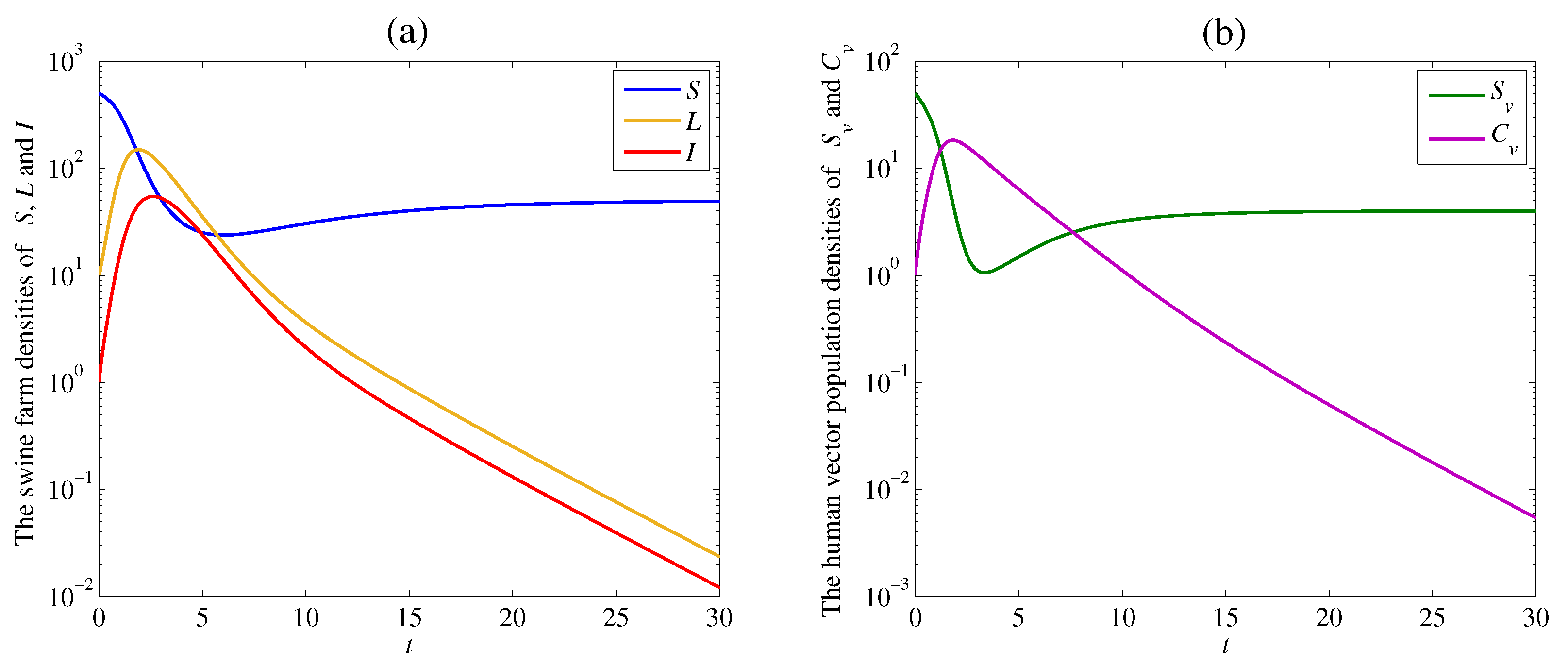
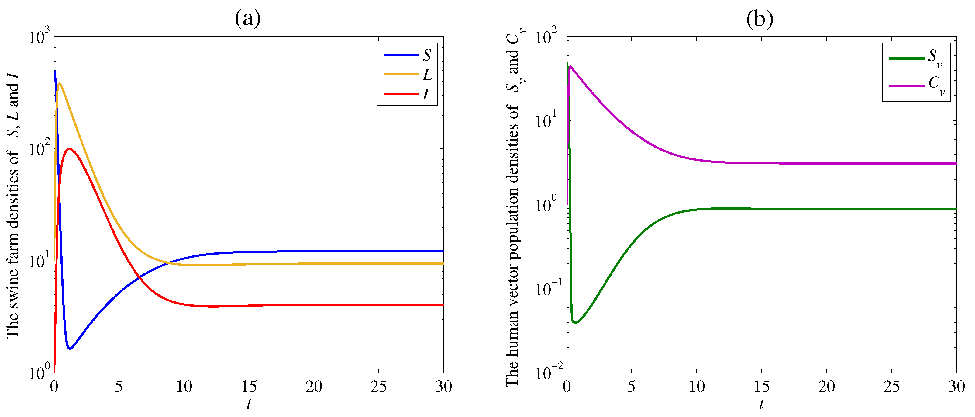
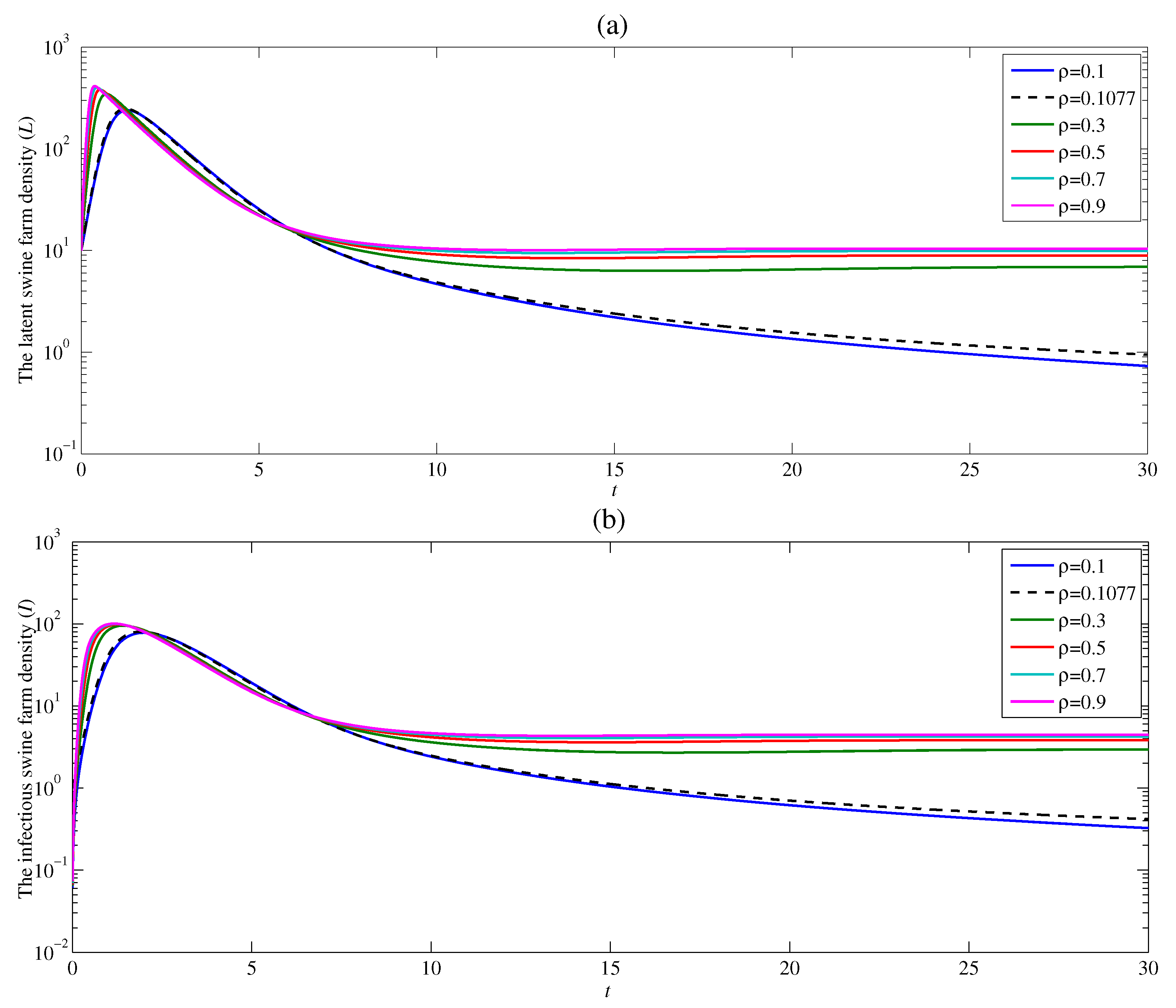
4. Numerical Examples and Discussion

The numerical results of the system (1) are computed by using MATLAB with the given initial values: $S\left(0\right)=500,L\left(0\right)=10,I\left(0\right)=1,S_v\left(0\right)=50,C_v\left(0\right)=1.$ The numerical results of the system (1) with the parameter values as shown in

Table 1. Parameter values of the system (1).

Parameter	Value
$\Lambda$	10
$\mu$	0.2
$\eta$	0.6
$\gamma$	0.8
$\omega$	0.4
${\Lambda }_v$	2
$\sigma$	0.5

.

The solution trajectories satisfying Theorem 3 with the remaining parameter values $\rho =0.05,\alpha =0.01,$ and $\beta =0.01$ tend to the disease-free equilibrium $\left(E^0\right)$ as shown in Figure 2. The calculated reproduction number of this case is $R_0=0.3571<1.$

As a result, the densities of the susceptible swine farm $\left(S\right)$ and the susceptible human vector $\left(S_v\right)$ dramatically decrease at the beginning of the outbreak. After that, they slightly increase and tend to positive equilibrium numbers $S^0$ and $S_v^0$ due to the optimal disease control. On the other hand, the densities of the latent swine farm $\left(L\right)$, the infectious swine farm $\left(I\right)$, and the contaminated human vector $\left(C_v\right)$ increase when the spread of the disease occurs. Then, they approach zero since the disease dies out, as shown in Figure 2a,b.

The solution trajectories tend to the endemic equilibrium $\left(E^{*}\right)$ which satisfy Theorem 4 with the remaining parameter values $\rho =0.2,\alpha =0.1,$ and $\beta =0.2$ as shown in Figure 3. The calculated reproduction number of this case is $R_0=18.5714>1.$

The densities of the susceptible swine farm $\left(S\right)$ and the susceptible human vector $\left(S_v\right)$ dramatically decrease at the beginning of the outbreak. Then, these densities gently increase and approach positive equilibrium numbers $S^0$ and $S_v^0$ similar to the previous case. However, the densities of the latent swine farm $\left(L\right)$, the infectious swine farm $\left(I\right)$, and the contaminated human vector density $C_v$ are high and steep when the disease cannot be controlled. Finally, the solution trajectories approach positive values since the disease still appears in both swine farms and human vectors, as shown in Figure 3a,b.

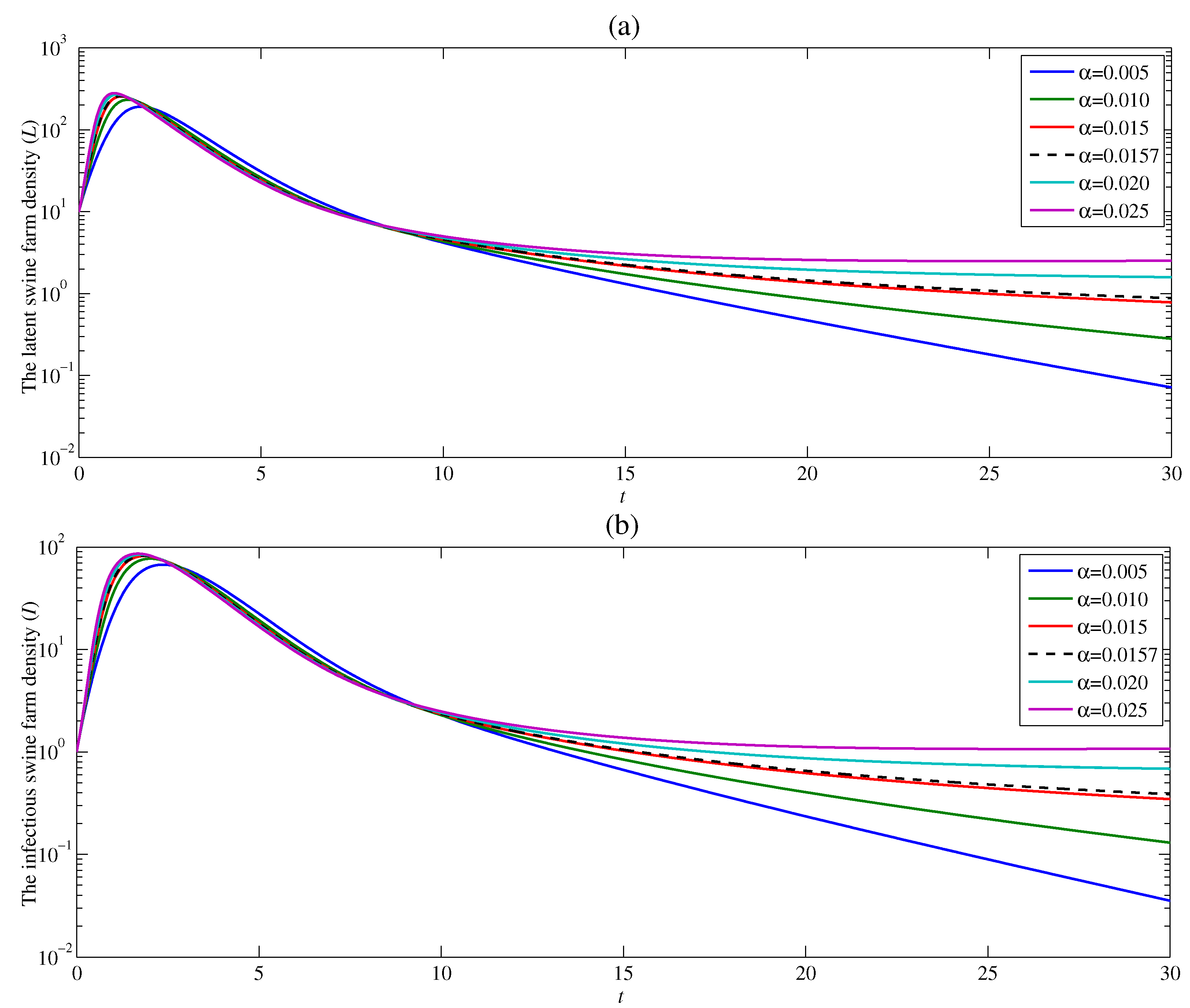
4.1. The Effect of the Contacting Human Vector Rate $\rho$

The dynamic of ASF is studied in five different contact rates $\rho =0.1,0.3,0.5,0.7,$ and $0.9$ with $\alpha =0.01$ and $\beta =0.02$. Figure 4a shows that the density of the latent swine farm sharply rises at the beginning time, and then dramatically drops for all contact rates $\rho$. With the constant rate $\rho =0.9$, the latent swine farm density is around 15 as time t approaches infinity. This means the ASF endemic still exists. The density of the latent swine farm decreases at a higher rate as the contact rate $\rho$ decreases. Additionally, if the value of the contact rate $\rho$ is low enough $(\rho <0.1077)$ resulting in $R_0<1$, the latent swine farm density continuously falls off as t approaches infinity. Since the latent swine farm density drops to zero, the endemic is over. The similar result for the density of infectious swine farms can be observed in Figure 4b. As a result, the contact rate $\rho$ significantly affects both latent and infectious swine farm densities. Moreover, this result confirms that the basic reproduction number $R_0$ obtained in Section 3 varies directly as $\rho$. Therefore, when $R_0<1$, the contact rate $\rho$ between susceptible swine farm and contaminated human should be as low as possible for the disease to die out.

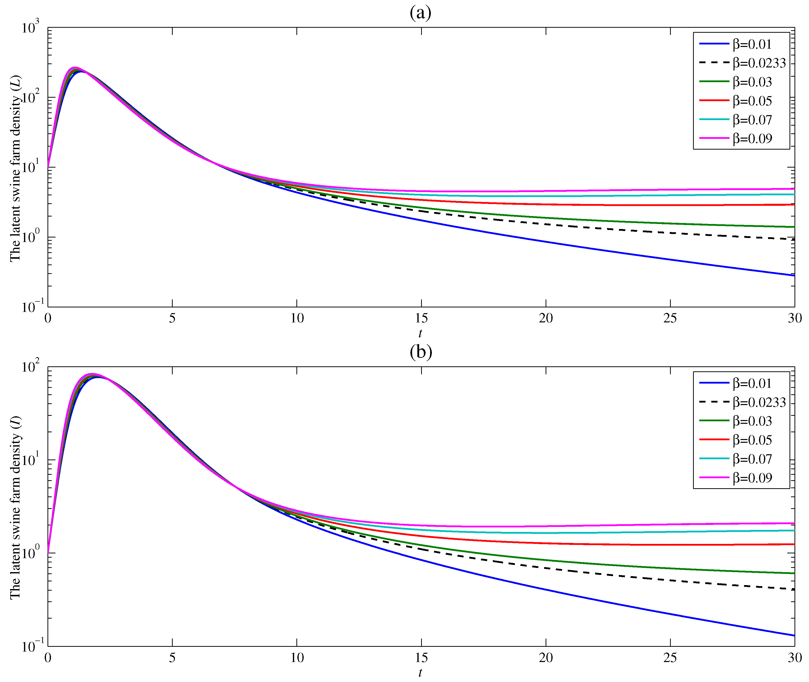
4.2. The Effect of the Contacting Human Vector Rate $\alpha$

Figure 5 presents the effect of the contact rate $\alpha$ between the susceptible human vector and the latent swine farm on ASF endemic. The study has been carried out with five given values of $\alpha =0.005,0.010,0.015,0.020,$ and $0.025$ with $\rho =0.1$ and $\beta =0.01$. It can be observed that after the peak, the densities of the latent swine farm and infectious swine farm drastically decrease as time increases. Moreover, the latent and infectious swine farm densities as t goes to infinity approach a lower value when $\alpha$ decreases. Indeed, the latent and infectious swine farm densities approach a positive number when $\alpha >0.0157$$(R_0>1)$, but approach zero when $\alpha <0.0157$$(R_0<1)$. Consequently, it can be interpreted that the endemic of ASF is more controllable when the contact between susceptible human vector and latent swine farm is restricted. This result is also consistent with the analytical basic reproduction number $R_0$ in Section 3, i.e., $R_0$ increases with an increase in $\alpha$.

4.3. The Effect of the Contacting Human Vector Rate $\beta$

The variation of swine farm density against time is demonstrated in Figure 6 using the following values of contact rates between susceptible human vector and infectious swine farm $\beta =0.01,0.03,0.05,0.07,$ and $0.09$ with $\rho =0.1$ and $\alpha =0.01$. The result illustrates the changes in the latent and infectious swine farm densities analogous to the pattern of densities showing the effect of $\rho$ (Figure 4) and $\alpha$ (Figure 5). Hence, the contact rate $\beta$ plays a significant role in the ASF endemic. The less the contact between susceptible human vector and infectious swine farm, the better the ASF endemic situation. This consequence agrees with the analytical basic reproduction number $R_0$ that is, $R_0$ increases with an increase in $\beta$.

5. Conclusions

We propose the novel mathematical model of ASF endemic by considering the swine population as an individual farm instead. This consideration should yield a more realistic situation in the ASF endemic since a swine farm is usually located separately from others, and ASF spreads very rapidly inside a swine farm. In this study, the ASF transmission is caused by a contaminated human. The results show that the contact between humans and swine farms when one is infected or contaminated plays a crucial role in controlling the ASF endemic. Indeed, the lower the contact rates, the more controllable the endemic. Moreover, if the contact between humans and swine farms is restricted properly, the endemic will be under control and, eventually, end.

References

1. Dixon, L.K.; Stahl, K.; Jori, F.; Vial, L.; Pfeiffer, D.U. African Swine Fever Epidemiology and Control. Annu. Rev. Anim. Biosci. 2020, 8, 221–246. [Google Scholar] [CrossRef] [Green Version]
2. Blome, S.; Franzke, K.; Beer, M. African swine fever—A review of current knowledge. Virus Res. 2020, 287, 198099. [Google Scholar] [CrossRef]
3. United States Department of Agriculture. Factsheet—African Swine Fever. Available online: https://www.aphis.usda.gov/publications/animal_health/asf.pdf (accessed on 30 April 2022).
4. Bonnet, S.I.; Bouhsira, E.; De Regge, N.; Fite, J.; Etoré, F.; Garigliany, M.M.; Jori, F.; Lempereur, L.; Le Potier, M.F.; Quillery, E.; et al. Putative Role of Arthropod Vectors in African Swine Fever Virus Transmission in Relation to Their Bio-Ecological Properties. Viruses 2020, 12, 778. [Google Scholar] [CrossRef]
5. Niederwerder, M.C. Risk and Mitigation of African Swine Fever Virus in Feed. Animals 2021, 11, 792. [Google Scholar] [CrossRef]
6. World Organisation for Animal Health. What Is African Swine Fever? Available online: https://www.oie.int/en/disease/african-swine-fever/ (accessed on 30 April 2022).
7. Chenais, E.; Depner, K.; Guberti, V.; Dietze, K.; Viltrop, A.; Ståhl, K. Epidemiological considerations on African swine fever in Europe 2014–2018. Porc. Health Manag. 2019, 5, 6. [Google Scholar] [CrossRef]
8. Wu, K.; Liu, J.; Wang, L.; Fan, S.; Li, Z.; Li, Y.; Yi, L.; Ding, H.; Zhao, M.; Chen, J. Current State of Global African Swine Fever Vaccine Development under the Prevalence and Transmission of ASF in China. Vaccines 2020, 8, 531. [Google Scholar] [CrossRef]
9. Galindo, I.; Alonso, C. African Swine Fever Virus: A Review. Viruses 2017, 9, 103. [Google Scholar] [CrossRef] [Green Version]
10. Agriculture and Consumer Protection Department, Food and Agriculture Organization of the United Nations. ASF Situation in Asia & Pacific Update. Available online: https://www.swineweb.com/asf-situation-in-asia-pacific-update (accessed on 16 May 2022).
11. Turlewicz-Podbielska, H.; Kuriga, A.; Niemyjski, R.; Tarasiuk, G.; Pomorska-Mól, M. African Swine Fever Virus as a Difficult Opponent in the Fight for a Vaccine—Current Data. Viruses 2021, 13, 1212. [Google Scholar] [CrossRef]
12. Meloni, D.; Franzoni, G.; Oggiano, A. Cell Lines for the Development of African Swine Fever Virus Vaccine Candidates: An Update. Vaccines 2022, 10, 707. [Google Scholar] [CrossRef]
13. Nigsch, A.; Costard, S.; Jones, B.A.; Pfeiffer, D.U.; Wieland, B. Stochastic spatio-temporal modelling of African swine fever spread in the European Union during the high risk period. Prev. Vet. Med. 2013, 108, 262–275. [Google Scholar] [CrossRef]
14. Lee, H.S.; Thakur, K.K.; Pham-Thanh, L.; Dao, T.D.; Bui, A.N.; Bui, V.N.; Quang, H.N. A stochastic network-based model to simulate farm-level transmission of African swine fever virus in Vietnam. PLoS ONE 2021, 16, e0247770. [Google Scholar] [CrossRef] [PubMed]
15. Ndondo, A.; Kasereka, S.; Bisuta, S.; Kyamakya, K.; Doungmo, E.; Ngoie, R.B. Analysis, modeling and optimal control of COVID-19 outbreak with three forms of infection in Democratic Republic of the Congo. Results Phys. 2021, 24, 104096. [Google Scholar] [CrossRef] [PubMed]
16. Barongo, M.B.; Bishop, R.P.; Fèvre, E.M.; Knobel, D.L.; Ssematimba, A. A Mathematical Model that Simulates Control Options for African Swine Fever Virus (ASFV). PLoS ONE 2016, 11, e0158658. [Google Scholar] [CrossRef]
17. Nielsen, J.P.; Larsen, T.S.; Halasa, T.; Christiansen, L.E. Estimation of the transmission dynamics of African swine fever virus within a swine house. Epidemiol. Infect. 2017, 145, 2787–2796. [Google Scholar] [CrossRef] [Green Version]
18. Kouidere, A.; Balatif, O.; Rachik, M. Analysis and optimal control of a mathematical modeling of the spread of African swine fever virus with a case study of South Korea and cost-effectiveness. Chaos Solitons Fractals 2021, 146, 110867. [Google Scholar] [CrossRef]
19. Halasa, T.; Boklund, A.; Bøtner, A.; Toft, N.; Thulke, H.H. Simulation of Spread of African Swine Fever, Including the Effects of Residues from Dead Animals. Front. Vet. Sci. 2016, 3, 6. [Google Scholar] [CrossRef] [Green Version]
20. Mai, T.N.; Sekiguchi, S.; Huynh, T.M.L.; Cao, T.B.P.; Le, V.P.; Dong, V.H.; Vu, V.A.; Wiratsudakul, A. Dynamic Models of Within-Herd Transmission and Recommendation for Vaccination Coverage Requirement in the Case of African Swine Fever in Vietnam. Vet. Sci. 2022, 9, 292. [Google Scholar] [CrossRef]
21. Weiss, H.H. The SIR model and the foundations of public health. Mater. Mat. 2013, 2013, 1–17. [Google Scholar]
22. Chaiya, I.; Trachoo, K.; Nonlaopon, K.; Prathumwan, D. The Mathematical Model for Streptococcus suis Infection in Pig-Human Population with Humidity Effect. Comput. Mater. Contin. 2022, 71, 2981–2998. [Google Scholar] [CrossRef]
23. Acemoglu, D.; Chernozhukov, V.; Werning, I.; Whinston, M.D. Optimal targeted lockdowns in a multigroup SIR model. Am. Econ. Rev. Insights 2021, 3, 487–502. [Google Scholar] [CrossRef]
24. Prathumwan, D.; Trachoo, K.; Chaiya, I. Mathematical Modeling for Prediction Dynamics of the Coronavirus Disease 2019 (COVID-19) Pandemic, Quarantine Control Measures. Symmetry 2020, 12, 1404. [Google Scholar] [CrossRef]
25. Ji, C.; Jiang, D. Threshold behaviour of a stochastic SIR model. Appl. Math. Model. 2014, 38, 5067–5079. [Google Scholar] [CrossRef]
26. Derrick, N.; Grossman, S. Differential Equation with Application; Addision Wesley Publishing Company, Inc.: Reading, MA, USA, 1976. [Google Scholar]
27. van den Driessche, P.; Watmough, J. Reproduction numbers and sub-threshold endemic equilibria for compartmental models of disease transmission. Math. Biosci. 2002, 180, 29–48. [Google Scholar] [CrossRef]
28. Diekmann, O.; Heesterbeek, J.A.P.; Roberts, M.G. The construction of next-generation matrices for compartmental epidemic models. J. R. Soc. Interface 2010, 7, 873–885. [Google Scholar] [CrossRef] [Green Version]
Figure 1. Flowchart of SLI-SC (Susceptible-Latent-Infectious-Susceptible-Contaminated) model for swine and human vector.
Axioms 11 00329 g001
Figure 2. Simulation results of the system (1): (a) the time series of the susceptible swine farm density ( S ) , the latent swine farm density ( L ) , and the infectious swine farm density ( I ) ; (b) the time series of the susceptible human vector population density ( S v ) , and the contaminated human vector population density ( C v ) . The solution trajectory tends toward the disease free equilibrium ( E 0 ) when R 0 < 1 .
Axioms 11 00329 g002
Figure 3. Simulation results of system (1): (a) the time series of susceptible swine farm density ( S ) , latent swine farm density ( L ) , and infectious swine farm density ( I ) ; (b) the time series of susceptible human vector population density ( S v ) , and contaminated human vector population density ( C v ) . The solution trajectory tends toward the endemic equilibrium ( E * ) when R 0 > 1 .
Axioms 11 00329 g003
Figure 4. Changes in (a) the latent swine farm density L ( t ) and (b) the infectious swine farm density I ( t ) with time at various value of ρ .
Axioms 11 00329 g004
Figure 5. Changes in (a) the latent swine farm density L ( t ) and (b) the infectious swine farm density I ( t ) with time at various value of α .
Axioms 11 00329 g005
Figure 6. Changes in (a) the latent swine farm density L ( t ) and (b) the infectious swine farm density I ( t ) with time at various value of β .
Axioms 11 00329 g006