
Exponential Multistep Methods for Stiff Delay Differential Equations


School of Mathematics and Statistics, Guangdong University of Technology, Guangzhou 510006, China
*
Author to whom correspondence should be addressed.
Axioms 2022, 11(5), 185; https://doi.org/10.3390/axioms11050185
Submission received: 25 March 2022
/
Revised: 15 April 2022
/
Accepted: 18 April 2022
/
Published: 19 April 2022
(This article belongs to the Special Issue Numerical Computation, Approximation of Functions and Applied Mathematics)
Abstract
:Stiff delay differential equations are frequently utilized in practice, but their numerical simulations are difficult due to the complicated interaction between the stiff and delay terms. At the moment, only a few low-order algorithms offer acceptable convergent and stable features. Exponential integrators are a type of efficient numerical approach for stiff problems that can eliminate the influence of stiffness on the scheme by precisely dealing with the stiff term. This study is concerned with two exponential multistep methods of Adams type for stiff delay differential equations. For semilinear delay differential equations, applying the linear multistep method directly to the integral form of the equation yields the exponential multistep method. It is shown that the proposed k-step method is stiffly convergent of order k. On the other hand, we can follow the strategy of the Rosenbrock method to linearize the equation along the numerical solution in each step. The so-called exponential Rosenbrock multistep method is constructed by applying the exponential multistep method to the transformed form of the semilinear delay differential equation. This method can be easily extended to nonlinear delay differential equations. The main contribution of this study is that we show that the k-step exponential Rosenbrock multistep method is stiffly convergent of order within the framework of a strongly continuous semigroup on Banach space. As a result, the methods developed in this study may be utilized to solve abstract stiff delay differential equations and can be served as time matching methods for delay partial differential equations. Numerical experiments are presented to demonstrate the theoretical results.
Keywords:
stiff delay differential equations; exponential multistep methods; Rosenbrock methods; convergenceMSC:
65L04; 65L06; 65L201. Introduction
Delay differential equations (DDEs) have received substantial attention in recent decades. They are used to model many systems in science and engineering. In these systems, the change of the unknown quantity depends not only on the present state but also on the past state. A typical DDE takes the form of
where stands for the past effects, and is the time lag. Such equations arise in various fields such as biology [1], control theory [2], population dynamics [3], and others [4,5,6,7].
To solve delay differential equations numerically, the intuitive approach is to use the mature method for ordinary differential equations (ODEs). Many numerical methods originally designed for ODEs have been applied to DDEs. The reader is referred to the monograph by Bellen and Zennaro [8] for a comprehensive review.
In the last few years, exponential integrators have been getting a lot of attention in the field of numerical solutions of ODEs. Exponential integrators eliminate the influence of stiffness on the scheme by handling the stiff term precisely. The first two exponential integrators of order two and three based on the Adams–Moulton method have been presented in [9]. Along with improving computational efficiency, considerable effort has been directed at developing and analyzing exponential integrators for semilinear stiff ODEs. Various exponential integrators have been investigated, such as exponential Runge–Kutta methods [10,11], exponential multistep methods [12,13], exponential Rosenbrock methods [14,15,16], exponential Taylor methods [17], and exponential general linear methods [18]. A good exposition of exponential integrators can be found in [19].
However, a large number of numerical findings demonstrate that, when a method designed for ODEs is directly applied to the DDEs, the method’s accuracy and stability properties cannot be maintained. The majority of current theoretical results on the convergence and stability of the classic methods have the following shortcomings. To preserve the stiff convergent order of the original numerical methods for ODEs, the addition of delay terms necessitates that the method fulfills more stiff convergence order conditions. Moreover, the method’s stability conditions get more complicated. More and stronger stability conditions are required to ensure that the scheme meets certain stability requirements. Integration of DDEs requires specifically designed methods other than the stand ODE methods. Furthermore, the stability and convergence properties of numerical methods should be thoroughly investigated.
Analysis of exponential integrators to DDEs has been addressed in the literature. In [20], D–convergence and conditional GDN–the stability of implicit exponential Runge–Kutta methods have been studied for semilinear DDEs. For exponential Runge–Kutta methods, the sufficient conditions of D–convergence and conditional GDN–stability given in [20] imply that the method must be implicit. In [21,22], the stiff convergence and conditional DN–stability of explicit exponential Runge–Kutta methods have been investigated for stiff DDEs. In view of the excellent properties of exponential integrators, the motivation of this work is to develop efficient exponential integrators for DDEs. We aim to construct exponential integrators that have fewer restrictions.
This study is concerned with two exponential multistep methods of Adams type for stiff delay differential equations. For semilinear delay differential equations, applying the linear multistep method directly to the integral form of the equation yields the exponential multistep method. It is shown that the proposed k-step method is stiffly convergent of order k. On the other hand, we can follow the strategy of the Rosenbrock method to linearize the equation along the numerical solution in each step. The so-called exponential Rosenbrock multistep method is constructed by applying the exponential multistep method to the transformed form of the semilinear delay differential equation. This method can be easily extended to nonlinear delay differential equations. The main contribution of this work is that we show that the k-step exponential Rosenbrock multistep method is stiffly convergent of order because of the favorable features of the transformed form. The novelty of this study is that the presented methods have fewer restriction conditions than classical linear multistep methods. Moreover, the convergence analysis is carried out within the framework of a strongly continuous semigroup on Banach space. As a result, the methods developed in this study may be utilized to solve abstract stiff delay differential equations and can be served as time matching methods for delay partial differential equations.
The paper is outlined as follows: in Section 2, exponential multistep methods are constructed for semilinear DDEs. It is shown that the proposed k-step method is stiffly convergent of order k. Section 3 is devoted to the exponential Rosenbrock multistep methods. Based on the interpolation with a Hermite node at the beginning of each step, the k-step exponential Rosenbrock multistep method is shown to be stiffly convergent of order . Finally, numerical experiments are shown to demonstrate the theoretical findings.
2. Exponential Multistep Methods
In this section, we consider the following semilinear delay differential equation:
This form may arise from the space discretization of some semilinear delay parabolic equations [15]. In this case, is the unknown function, A is a given matrix in , and g is a nonlinear continuous function. The methods presented in this paper are also applicable to abstract delay differential equations in certain Banach space X with norm . In this instance, and A is a linear operator (can be unbounded) from X to X.
2.1. Construction of Exponential Multistep Methods
We divide the interval by time step size h and denote ; then, for a given integer s, applying the variation-of-constants formula to Equation (1) yields
This is the starting point of the exponential multistep methods. Let denote the approximation of exact solution at time . Similarly, is the numerical solution at . Exponential multistep methods are constructed by treating the integral part in (2) numerically.
We approximate the nonlinear term g in Equation (2) by the Lagrange interpolation polynomial through the points
Here, we set for simplicity. According to the Newton backward interpolation formula, the polynomial can be expressed as follows:
Here, denotes the jth backward difference, defined recursively by
Note that the delay terms are involved in the interpolation data . For , we can simply set by the initial function, i.e., . When , we approximate it by the Lagrange interpolation polynomial through points
Here, integer m satisfies . is required to ensure that no unknown values are used. The Lagrange interpolation polynomial can be expressed as follows:
We now have all of the pieces necessary to construct the exponential multistep methods. This paper focuses on multistep methods of Adams type; hence, we set in (2). The numerical method is obtained by replacing the nonlinearity g in (2) by the interpolation polynomial . Therefore, we can write
then, we have the k-step exponential multistep method for semilinear DDEs (1)
The weights are defined as
Remark 1.
We remark that the proposed method can be viewed as a small perturbation of the exponential Euler method, which is given by
The weights given in (5) can be expressed as the linear combination of -functions, which are defined as follows:
Definition 1.
For any complex numbers , let . For all integers , define as
Note that -functions enjoy the following recurrence relation:
By introducing the -functions, the weights of the k-step exponential multistep methods up to are given by
Remark 2.
It is obvious that efficiently computing the φ-functions is critical for the implementation of exponential multistep methods. Several efforts have been made on this line; see [23,24,25,26]. For large-scale problems, it is more efficient to compute the product of a matrix exponential function with a vector directly without the explicit form of the matrix exponential.
Remark 3.
For multistep methods, the starting values are unknown. Normally, they are obtained by one-step methods. Here, we take the method proposed in [12]. The details are listed in Appendix A.
2.2. Stiff Convergence of Exponential Multistep Methods
In this subsection, we investigate the stiff convergence of the k-step exponential multistep method (4). Stiff convergence refers to the error bounds being of form , where the constant C is independent of the stiffness and the step size h. The analysis is carried out under the framework of semigroup. The following assumptions on the semilinear DDEs (1) are suggested.
Assumption 1.
Let X be a Banach space with norm . The solution of Equation (1) is sufficiently smooth. The linear operator is the infinitesimal generator of a strongly continuous semigroup on X. The nonlinearity is Frechet differentiable in a strip along the exact solution . All occurring derivatives are supposed to be uniformly bounded.
Under this assumption, there exists a Lipschitz constant L such that
holds in a neighborhood of the exact solution. Moreover, the following parabolic smoothing property holds:
For the functions defined by (6), we have
It follows that the weights are bounded operators.
The main result is the following.
Theorem 1.
Proof.
Let denote the error of the method at time . It is easy to see that . The first step is to build the error equation for .
Note that the exact solution of (1) has the similar form as the numerical solution . Indeed, according to the variation-of-constants formula, the solution of (1) has the form
with for simplicity. Denote as the interpolation polynomial through the exact data
It easily follows that
and the interpolation error is
Here, the defect is
Solving this recursion with , we find that
We will now show that the error indeed satisfies the bound (9).
Next, we have to estimate the term . Note that functions and contain the information of the delay terms. To this end, let denote the interpolation polynomial through the exact history data
Then, there exists a polynomial of degree such that
where . Similarly, in the case of , we see that
Now, we are in the position to estimate the error .
Combining the above estimation with (13) yields
Here, the bound (8) is involved. Using the discrete Gronwall’s lemma, we have
The assertion is obtained by setting . □
3. Exponential Rosenbrock Multistep Methods
In the last section, we designed the exponential multistep methods for semilinear DDEs and investigated their stiff convergence. However, in some instances, the numerical results indicate that this treatment may cause certain issues. Especially when the initial state is far from the equilibrium point, the scheme must take a very tiny time step to make sure it stays stable. This reduces the method’s computational efficiency.
In this section, we follow the strategy of the Rosenbrock method [14] to linearize the equation along the numerical solution in each step. The so-called exponential Rosenbrock multistep method is constructed by applying the exponential multistep method to the transformed form of the delay differential equation. This method can be easily extended to nonlinear delay differential equations. Furthermore, we can show that the k-step exponential Rosenbrock multistep method is stiffly convergent of order because of the favorable features of the transformed form.
3.1. Construction of Exponential Rosenbrock Multistep Methods
To advance the semilinear DDE (1) from to , we perform the following transformation based on the state . Let d, J, and be the Jacobians of the right-hand side of Equation (1) with respect to the first term t, the second term y, and the third term , respectively, i.e.,
We evaluate at state and denote by
Then, we rewrite the semilinear DDE (1) as
Here, the reminder is given by
It enjoys
As will be indicated in Section 3.2, these properties are critical in deriving the convergence order of the exponential Rosenbrock multistep method.
Remark 4.
It appears that the semilinear DDE has been changed into a more complicated form. Nevertheless, the Lipschitz constant of the remainder in (14) is smaller than that of the nonlinear term g in (1). The numerical results presented in Section 4 indicate that the exponential multistep method based on (14) is more accurate than that based on the original form (1). Indeed, we will show that the k-step exponential Rosenbrock multistep method is stiffly convergent of order . The order of this method is higher than that of the exponential multistep method.
We now construct the exponential Rosenbrock multistep method for semilinear DDE (1) based on the form (14).
The exact solution of (14) can be expressed by the following variation-of-constants formula:
With the -functions defined by (6), we arrive at
The exponential Rosenbrock multistep method is obtained by replacing and with suitable approximations.
For , we use the interpolation polynomial through points
and evaluate it at . That is,
For the reminder term , we approximate it by the interpolation polynomial through points
Noting the property (15), for the given data, we have . Hence, we further require that . In other words, we employ an incomplete Hermite interpolation to approximate . This is the source for the order convergent of a k-step exponential Rosenbrock multistep method. Denoting for simplicity, the Hermite interpolation polynomial reads
Replacing the delay term and the reminder term in (16) by polynomials and , respectively, gives
This is the exponential Rosenbrock multistep method for semilinear DDE (1). The procedure for determining the stating values are sketched in Appendix B.
Remark 5.
The exponential multistep method can be easily extended to a nonlinear delay differential equation
The exponential Rosenbrock multistep method is based on the transformed form
with the corresponding reminder . All of the derivatives take values at state .
3.2. Stiff Convergence of Exponential Rosenbrock Multistep Methods
This subsection is devoted to investigating the stiff convergence of the exponential Rosenbrock multistep methods for semilinear DDEs (1).
Under Assumption (1), these Jacobians satisfy the Lipschitz condition:
Note that the nonlinear operator J can be viewed as a perturbation of g. We infer from Assumption (1) and the perturbation result in [27] that J generates a strongly continuous semigroup . Hence, there exist constants , such that
hold uniformly in a neighborhood of the exact solution. It further implies that and are bounded operators. Indeed, we have
We are now in a position to state our main result on the convergence of the exponential Rosenbrock multistep methods. In contrast to the case of exponential multistep methods, the Jacobians vary with each step. Hence, the proof is more involved.
Theorem 2.
Proof.
Let denote the error of the method at time .
The semilinear DDE (1) are recast into the form of (14) at . Then, the variation-of-constants formula allows us to write the solution of (14) as
with for simplicity.
For , we consider the Hermite interpolation polynomial through the exact data
and satisfies . Then, the interpolation error can given by
Here, is a certain intermediate time in the interval .
On the other hand, for delay term , we introduce the interpolation polynomial based on the exact data
In this case, we have the interpolation error
for certain intermediate time .
Replacing the nonlinearity term and the delay term in (19) by and respectively yields
This means that the exact solution can be expressed in a similar form as the numerical solution. Here, the defects and are
Solving this recursion and using gives
To bound the terms and in error Equation (21), we proceed in the same manner as for the term in Theorem 1. In fact, we have
and
Here, we have taken .
The result follows now from the application of the discrete Gronwall’s lemma. This completes the proof. □
4. Numerical Experiments
In this section, we present some experiments to demonstrate the theoretical results.
Example 1.
We consider the following semilinear delay reaction diffusion equation on interval
where D is the diffusion coefficient, σ, a, b, and c are positive constants. The added term is specified so that the exact solution is .
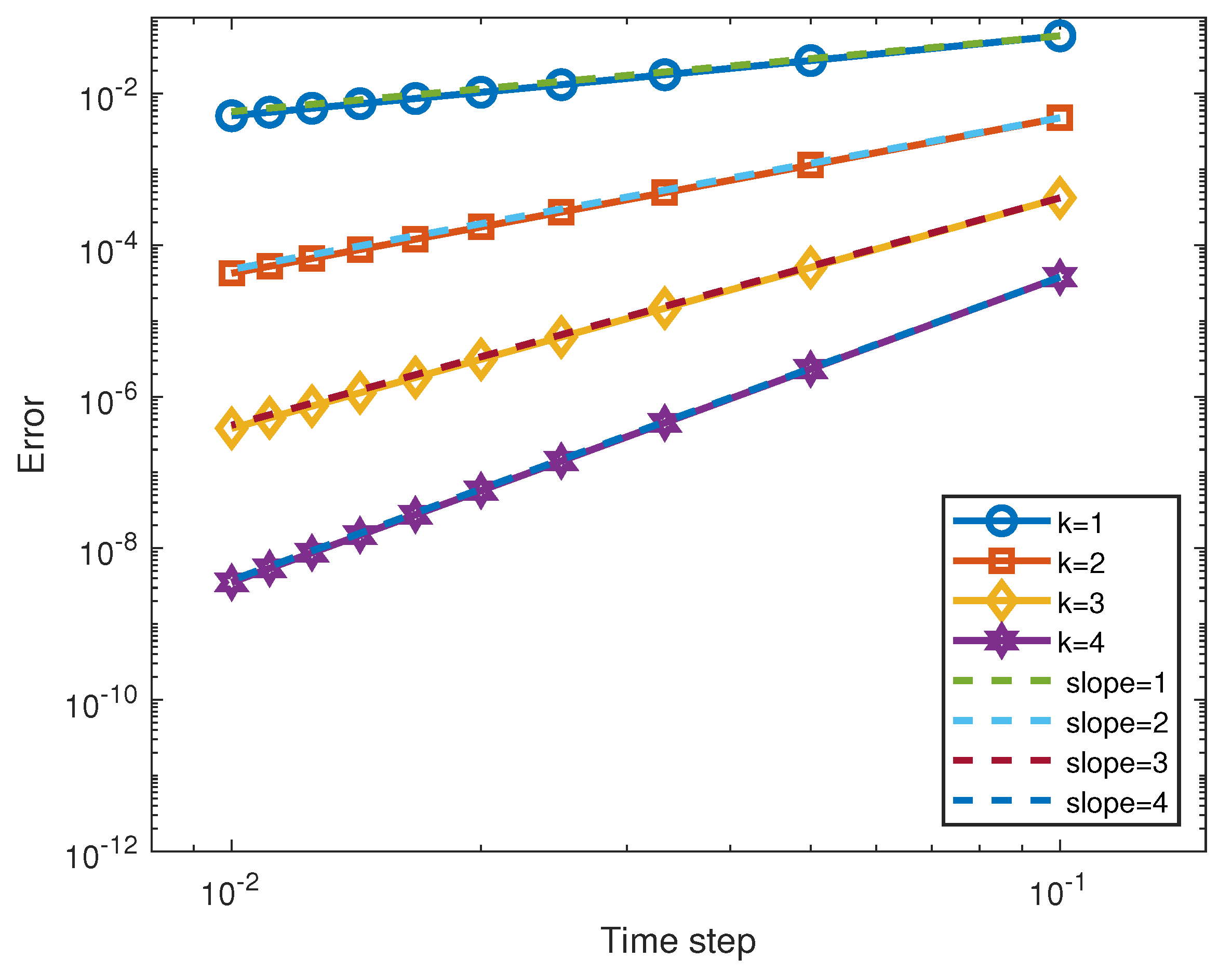
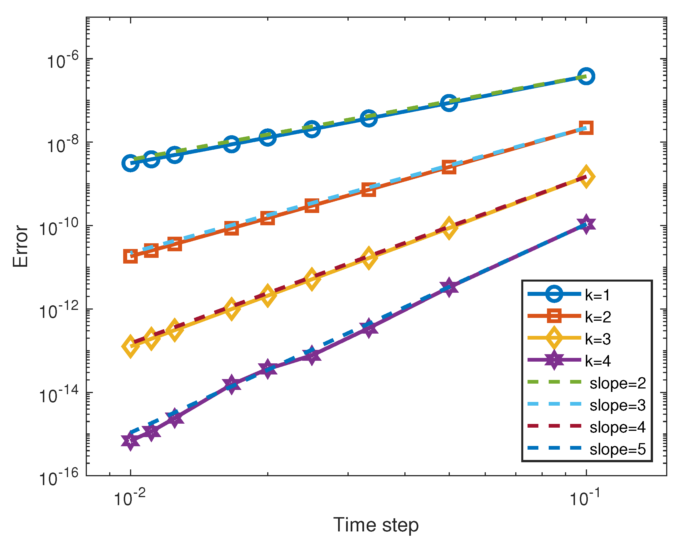
The space derivative is approximated by the standard second order central difference method with the mesh size of . For time discretization, the exponential multistep method (4) and the exponential Rosenbrock multistep method (17) are employed. The relative errors of the proposed methods are displayed in Figure 1 and Figure 2. We conclude that the k-step exponential multistep method gives a kth order of accuracy, while the k-step exponential Rosenbrock multistep method provides an accuracy of order . Moreover, the error of the exponential Rosenbrock multistep method is smaller than that of the exponential multistep method when the step size is the same.
To demonstrate the superiority of the proposed exponential methods over the classical methods, we measure the computing times of different methods. Adams linear multistep methods (see, e.g., [28]), exponential multistep methods, and exponential Rosenbrock multistep methods are compared in terms of computational times. The CPU times in seconds when all of the methods achieve a common error tolerance are recorded in Table 1. The results reported here show that exponential methods are more efficient than linear multistep methods. Furthermore, the advantages of high order methods over low order methods are proven clearly.
Example 2.
Next, we consider the following reaction diffusion system with delay
We solve this problem on with initial conditions
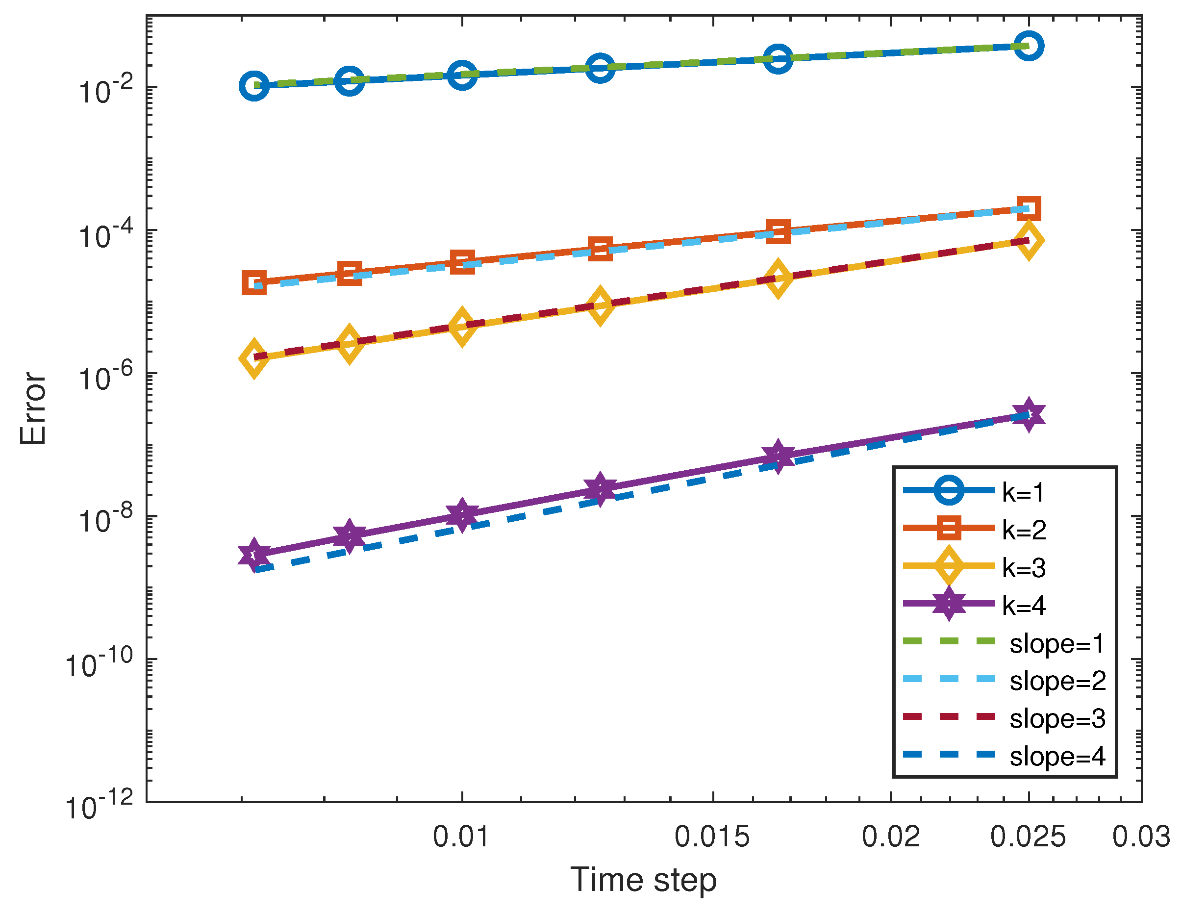
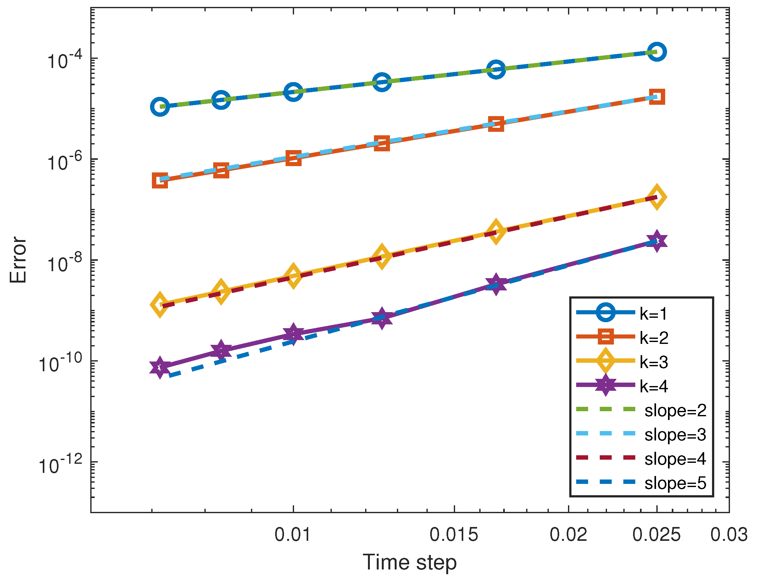
The numerical solutions are obtained by the methods used in Example 1. The relative errors are presented in Figure 3 and Figure 4. Clearly, all the methods achieve their theoretical convergence order. It also confirms that the exponential Rosenbrock multistep methods are more accurate than the exponential multistep methods.
5. Conclusions
In this paper, we propose the Adams type exponential multistep methods for semilinear stiff delay differential equations. The exponential multistep methods are obtained by applying the linear multistep method directly to the integral form of the equation, while the exponential Rosenbrock multistep methods are constructed by applying the exponential multistep methods to a transformed form of the equation. We show that the k-step exponential multistep method is stiffly convergent of order k and the stiff convergence order of the k-step exponential Rosenbrock multistep method is . We demonstrate that the exponential Rosenbrock multistep methods are superior to the exponential multistep methods in terms of accuracy. In summary, for semilinear stiff delay differential equations, this work provided efficient numerical methods with fewer restriction conditions.
Finally, we point out that, while the proposed exponential Rosenbrock multistep methods can be easily applied to nonlinear DDEs, the convergence analysis is restricted to semilinear stiff DDEs. The convergence property of the methods for nonlinear DDEs should be investigated in future research. Moreover, fractional [29] and stochastic [30] differential equations are also widely used in a variety of fields of applied mathematics. The exponential integrators for these problems need to be validated in the future.
Author Contributions
Conceptualization, R.Z. (Rui Zhan) and R.Z. (Runjie Zhang); methodology, R.Z. (Rui Zhan); software, W.C.; validation, X.C.; formal analysis, R.Z. (Rui Zhan); writing—original draft preparation, W.C. and X.C.; writing—review and editing, R.Z. (Rui Zhan) and R.Z. (Runjie Zhang). All authors have read and agreed to the published version of the manuscript.
Funding
This research was funded by the National Natural Science Foundation of China under Grant No. 12001115.
Data Availability Statement
Not applicable.
Conflicts of Interest
The authors declare no conflict of interest.
Appendix A
To determine the starting values for a k-step exponential multistep method, we approximate g in the integral form (2) by the interpolation polynomial through the points , , …, . Then, we have
Here, denotes the jth forward difference, which defined recursively by
Replacing g by polynomial gives the desired starting values
The coefficients are defined as
Appendix B
For the exponential Rosenbrock multistep method (17), the starting values are approximated by replacing the nonlinearity in (16) by the Hermite interpolation polynomial , namely, by
Together with the interpolation polynomial for , for the starting value is computed by
References
- MacDonals, N. Biological Delay Systems: Linear Stability Theory; Cambridge University Press: Cambridge, UK, 1989. [Google Scholar]
- Hu, H. Dynamics of Controlled Mechanical Systems with Delayed Feedback; Springer: New York, NY, USA, 2002. [Google Scholar]
- Kuang, Y. Delay Differential Equations with Applications in Population Dynamics; Academic: Boston, MA, USA, 1993. [Google Scholar]
- Stépán, G. Retarded Dynamical Systems: Stability and Characteristic Functions; Longman Scientific and Technical: Marlow, NY, USA, 1989. [Google Scholar]
- Hale, J. History of delay equations. In Delay Differential Equations and Applications; Arino, O., Hbid, M., Dads, E.A., Eds.; Springer: Amsterdam, The Netherlands, 2006; pp. 1–28. [Google Scholar]
- Abd-Rabo, M.A.; Zakarya, M.; Cesarano, C.; Aly, S. Bifurcation analysis of time-delay model of consumer with the advertising effect. Symmetry 2021, 13, 417. [Google Scholar] [CrossRef]
- Duary, A.; Das, S.; Arif, M.G.; Abualnaja, K.M.; Khan, M.A.A.; Zakarya, M.; Shaikh, A.A. Advance and delay in payments with the price-discount inventory model for deteriorating items under capacity constraint and partially backlogged shortages. Alex. Eng. J. 2022, 61, 1735–1745. [Google Scholar] [CrossRef]
- Bellen, A.; Zennaro, M. Numerical Methods for Delay Differential Equations; Oxford University Press: New York, NY, USA, 2003. [Google Scholar]
- Certaine, J. The solution of ordinary differential equations with large time constants. In Mathematical Methods for Digital Computers; Ralston, A., Wilf, H., Eds.; Wiley: New York, NY, USA, 1960; pp. 128–132. [Google Scholar]
- Hochbruck, M.; Ostermann, A. Explicit exponential Runge–Kutta methods for semilinear parabolic problems. SIAM J. Numer. Anal. 2005, 43, 1069–1090. [Google Scholar] [CrossRef] [Green Version]
- Hochbruck, M.; Ostermann, A. Exponential Runge–Kutta methods for parabolic problems. Appl. Numer. Math. 2005, 53, 323–339. [Google Scholar] [CrossRef] [Green Version]
- Calvo, M.P.; Palencia, C. A Class of Explicit Multistep Exponential Integrators for Semilinear Problems. Numer. Math. 2006, 102, 367–381. [Google Scholar] [CrossRef]
- Hochbruck, M.; Ostermann, A. Exponential multistep methods of Adams-type. BIT 2011, 51, 889–908. [Google Scholar] [CrossRef] [Green Version]
- Hochbruck, M.; Ostermann, A.; Schweitzer, J. Exponential Rosenbrock-type methods. SIAM J. Numer. Anal. 2009, 47, 786–803. [Google Scholar] [CrossRef]
- Luan, V.T.; Ostermann, A. Exponential Rosenbrock methods of order five—Construction, analysis and numerical comparisons. J. Comput. Appl. Math. 2014, 255, 417–431. [Google Scholar] [CrossRef]
- Luan, V.T.; Ostermann, A. Parallel exponential Rosenbrock methods. Comput. Math. Appl. 2016, 71, 1137–1150. [Google Scholar] [CrossRef]
- Koskela, A.; Ostermann, A. Exponential Taylor methods: Analysis and implementation. Comput. Math. Appl. 2013, 65, 487–499. [Google Scholar] [CrossRef]
- Ostermann, A.; Thalhammer, M.; Wright, W. A class of explicit exponential general linear methods. BIT 2006, 46, 409–431. [Google Scholar] [CrossRef]
- Minchev, B.; Wright, W. A Review of Exponential Integrators for First Order Semi-Linear Problems; Technical Report; Norwegian University of Science and Technology: Trondheim, Norway, 2005. [Google Scholar]
- Zhao, J.; Zhan, R.; Xu, Y. D-convergence and conditional GDN-stability of exponential Runge–Kutta methods for semilinear delay differential equations. Appl. Math. Comput. 2018, 339, 45–58. [Google Scholar] [CrossRef]
- Zhao, J.; Zhan, R.; Xu, Y. Explicit exponential Runge–Kutta methods for semilinear parabolic delay differential equations. Math. Comput. Simul. 2020, 178, 366–381. [Google Scholar] [CrossRef]
- Fang, J.; Zhan, R. High order explicit exponential Runge–Kutta methods for semilinear delay differential equations. J. Comput. Appl. Math. 2021, 388. [Google Scholar] [CrossRef]
- Moler, C.; Loan, C.V. Nineteen Dubious Ways to Compute the Exponential of a Matrix, Twenty-Five Years Later. SIAM Rev. 2003, 45, 3–49. [Google Scholar] [CrossRef]
- Al-Mohy, A.; Higham, N. Computing the action of the matrix exponential, with an application to the exponential integrators. SIAM J. Sci. Comput. 2011, 33, 488–511. [Google Scholar] [CrossRef]
- Jawecki, T. A study of defect-based error estimates for the Krylov approximation of ϕ-functions. Numer. Algorithms 2022, 90, 323–361. [Google Scholar] [CrossRef]
- Li, D.; Yang, S.; Lan, J. Efficient and accurate computation for the ϕ-functions arising from exponential integrators. Calcolo 2022, 59, 1–24. [Google Scholar] [CrossRef]
- Pazy, A. Semigroups of Linear Operators and Applications to Partial Differential Equations; Springer: New York, NY, USA, 1983. [Google Scholar]
- Hairer, E.; Norsett, S.; Wanner, G. Solving Ordinary Differential Equations. I. Nonstiff Problems; Springer Series in Computational Mathematics; Springer: Heidelberg, Germany; New York, NY, USA, 1993. [Google Scholar]
- Ali, K.K.; Mohamed, E.M.; Abd El salam, M.A.; Nisar, K.S.; Khashan, M.M.; Zakarya, M. A collocation approach for multiterm variable-order fractional delay-differential equations using shifted Chebyshev polynomials. Alex. Eng. J. 2022, 61, 3511–3526. [Google Scholar] [CrossRef]
- Ghany, H.A.; Ibrahim, M.Z.N. Generalized solutions of wick-type stochastic KdV-Burgers equations using exp-function method. Int. Rev. Phys. 2014, 8. [Google Scholar]
Figure 1.
Errors of k-step exponential multistep method for problem (23). . .
Figure 1.
Errors of k-step exponential multistep method for problem (23). . .

Figure 2.
Errors of k-step exponential Rosenbrock multistep method for problem (23). . .
Figure 2.
Errors of k-step exponential Rosenbrock multistep method for problem (23). . .

Figure 3.
Errors of k-step exponential multistep method for problem (24). . , .
Figure 3.
Errors of k-step exponential multistep method for problem (24). . , .

Figure 4.
Errors of k-step exponential Rosenbrock multistep method for problem (24). . , .
Figure 4.
Errors of k-step exponential Rosenbrock multistep method for problem (24). . , .


Table 1.
CPU times of all the methods achieving error tolerance for problem (23).
Table 1.
CPU times of all the methods achieving error tolerance for problem (23).
| Adams linear multistep methods | |||
| exponential multistep method | |||
| exponential Rosenbrock multistep method |
Publisher’s Note: MDPI stays neutral with regard to jurisdictional claims in published maps and institutional affiliations. |
© 2022 by the authors. Licensee MDPI, Basel, Switzerland. This article is an open access article distributed under the terms and conditions of the Creative Commons Attribution (CC BY) license (https://creativecommons.org/licenses/by/4.0/).
Share and Cite
MDPI and ACS Style
Zhan, R.; Chen, W.; Chen, X.; Zhang, R. Exponential Multistep Methods for Stiff Delay Differential Equations. Axioms 2022, 11, 185. https://doi.org/10.3390/axioms11050185
AMA Style
Zhan R, Chen W, Chen X, Zhang R. Exponential Multistep Methods for Stiff Delay Differential Equations. Axioms. 2022; 11(5):185. https://doi.org/10.3390/axioms11050185
Chicago/Turabian StyleZhan, Rui, Weihong Chen, Xinji Chen, and Runjie Zhang. 2022. "Exponential Multistep Methods for Stiff Delay Differential Equations" Axioms 11, no. 5: 185. https://doi.org/10.3390/axioms11050185
Note that from the first issue of 2016, this journal uses article numbers instead of page numbers. See further details here.