
Data Analysis Using a Coupled System of Ornstein–Uhlenbeck Equations Driven by Lévy Processes

1
Department of Mathematical Sciences, University of Texas at El Paso, El Paso, TX 79902, USA
2
Computational Science Program, University of Texas at El Paso, El Paso, TX 79902, USA
3
Department of Data Science, Ramapo College of New Jersey, Mahwah, NJ 07430, USA
*
Author to whom correspondence should be addressed.
Axioms 2022, 11(4), 160; https://doi.org/10.3390/axioms11040160
Submission received: 28 January 2022
/
Revised: 14 March 2022
/
Accepted: 16 March 2022
/
Published: 1 April 2022
(This article belongs to the Special Issue Financial Mathematics and Econophysics)
Abstract
:In this work, we have analyzed data sets from various fields using a coupled Ornstein–Uhlenbeck (OU) system of equations driven by Lévy processes. The Ornstein–Uhlenbeck model is well known for its ability to capture stochastic behaviors when used as a predictive model. There’s empirical evidence showing that there exist dependencies or correlations between events; thus, we may be able to model them together. Here we show such correlation between data from finance, geophysics and health as well as show the predictive performance when they are modeled with a coupled Ornstein–Uhlenbeck system of equations. The results show that the solution to the stochastic system provides a good fit to the data sets analyzed. In addition by comparing the results obtained when the BDLP is a process or an IG(a,b) process, we are able to deduce the best choice out of the two to model our data sets.
1. Introduction
Since it was proposed in the 1930s, the Ornstein–Uhlenbeck model has been used in many areas of application, including, but not limited to, fields such as health care [1], nanotechnology/thermodynamics [2], geophysics [3] and finance [4,5,6]. Unlike its original proposition, which involved a Brownian motion as its background driving process, there have been many extensions or modifications to it in order to truly capture the behavior of data sets, which otherwise could not be modeled rightly with Brownian motions [7,8]. Empirical results have shown evidence of non-Brownian behavior in many real-world complex systems [5,9,10]. In fact, according to [9], statistics of the Lévy type is a ubiquitous phenomenon observed in a wide variety of areas, including physics, seismology, engineering to mention a few. Lévy motions constitute one of the important and fundamental families of random motions, which, unlike Brownian motions, have stationary and independent increments.
Being able to understand and predict future behaviors of stock markets will, without any doubt, be beneficial to individual investors and economic policymakers. It is for this reason that there is always ongoing research into improving the forecasting models of financial stock markets [3,5,10,11]. It is also of little surprise that there arise some dependencies within stock markets. In studying market trends, one would realize more often than not a positive relationship in the movements of stock portfolios, such as the Dow Jones, the NASDAQ, the Russell, and the S&P500. With the knowledge of these dependencies, we model a stochastic system of equations driven by Lévy processes to predict future trends of the stock market from two different portfolios.
Earthquakes, rock slides, and volcanic eruptions are known to be deadly disasters, which, if not forecasted correctly in order for cities to take safety measures, can result in unprecedented losses to life and property. The 1989–1990 Eruption of Mount Redoubt in Alaska was reported to have caused damages worth USD 160 million plus an additional USD 80 million for two planes that flew over it [12]. Meanwhile, the 1964 rock slide of Mt Toc, Italy, was estimated to have destroyed property worth USD 200 million and the loss of 2000 lives [13]. The more recent earthquake in Tohoku, Japan, was believed to have resulted in 18,000 deaths. Knowing the possibility of such devastating losses explains the many research works devoted to forecasting such phenomena [10,13,14,15,16,17]. This work includes an application of the model using volcanic eruption data obtained from the Bezymianny seismic station.
In January 2020, the first case of COVID-19 infection was reported in the United States of America, and since then, the entire year of 2020 and parts of 2021 were devoted to battling the spread of the COVID-19 virus, which plagued the entire world for the entirety of the year 2020. In the wake of this unprecedented pandemic, many researchers around the world sought to model the spread of the COVID-19 virus in order to help officials understand the severity of the situation as well as enact preventive measures to control the spread [18,19,20,21]. In reading the literature on these models, we observed that most of these models were in the class of compartmental models, which are mostly deterministic. Introducing the stochasticity in the prediction of the spread of the COVID-19 disease has the advantage of causing the disease to die out in scenarios where deterministic models predict disease persistence.
The Ornstein–Uhlenbeck model and its variants have been used to analyzed various data sets in the literature [22,23,24]. In this work, we extend its application by developing an intrafield and interfield coupled system with both and background driving processes. In our model, we have also used the R package [25] to estimate the volatility parameters, which we use in the coupled Ornstein–Uhlenbeck system of equations.
A common factor among the data sets being analyzed are their direct impact on human lives and properties. A financial crush has the potential of crippling economies and increasing poverty; a volcanic eruption affects human lives and property; and a disease outbreak affects human lives. In [26], authors showed that how complexity science is essential in modeling these events, which translates to the saving of human lives and property.
In this work, we applied a coupled system of Ornstein–Uhlenbeck stochastic differential equations (SDE) driven by Lévy processes (BDLP) to model three different areas of application. The applications presented include applications to financial data, volcanic eruptions data, and the U.S.A. COVID-19 data. For the financial data, we consider the Dow Jones, the NASDAQ, the S&P500, and the Russel. The volcanic eruptions data were obtained from the Bezymianny seismic station and the COVID-19 data from the New York Times database.
Using the three data sets, we model four different applications. The first three we term as intra-dependent field applications, which implies modeling two data sets collected from the same field. The last application we term as an interdependent field application deals with modeling a combination of two different fields, which in this paper refers to modeling the financial data with the COVID-19 data. Various works in the literature have shown the occurrence of such phenomena, where the actions of one event trigger specific behaviors in another. In [13], the author presented scenarios where volcanic eruptions preceded an earthquake from up to 120 miles away. It goes without saying that the financial market was greatly affected in the wake of the COVID-19 pandemic. Our model derives the correlation parameter, which shows the correlation between the COVID-19 daily cases and deaths with the stock market, thus helping us model the two different fields of data sets with one system of SDE.
For the BDLP, we consider two Lévy processes, namely the process and the IG(a,b) process. This affords us the ability to compare model performance based on the choice of BDLP to ascertain the desirable option.
The outline of the paper is as follows, we introduce the coupled system of Ornstein–Uhlenbeck equations in Section 2 in addition to the and the inverse Gaussian(a,b) process. In Section 3, we present the data used in addition to the estimation of relevant parameters from the data. Section 4 deals with the four different applications of our model and presents results from running simulations on the data using the model. We show the estimated errors when our model is used for predictions. In Section 5, we discuss the results observed from our simulation in Section 4, and finally, in Section 6, we present some conclusions as well as possible future works based on the current work and its results.
2. Model
Assume two stochastic (, ) processes relative to two time series data collected within a specified time period. Suppose the data sets have some correlation, i.e., their correlation coefficient is non-zero. We further assume the stochastic processes to be Lévy driven and simulate the model using either a process or an IG(a,b) process for comparison purposes. Then, we can model a coupled system of Ornstein–Uhlenbeck SDE as shown below in Equations (1) and (2)
where and are the intensity parameters, and determine volatility, and and describe the correlation between the data sets. Now, we observe that when , we end up with a decoupled system and thus conclude that the two occurrences do not have any correlation. When , we end up with a decoupled deterministic system, and each equation can be solved independently. and are the background driving Lévy processes for the system; we assume both and are either processes or IG(a,b) processes.
In matrix form, the system of the OU equation can be written as
where
and
The solution to this system was obtained in [5] with a clear step-by-step proof, and hence the proof is omitted in this work. The solution is thus given as
2.1. and IG(a,b) Process
In this section, we briefly define the process and the IG(a,b) process.
2.1.1. Process
Definition 1.
The gamma process is a stochastic process X = with parameters a and b which satisfies the following conditions:
- .
- The process has independent increments.
- For , the random variable has a distribution.
A random variable X has a gamma distribution with rate and shape parameters, and , respectively, if its density function is given by
2.1.2. IG(a,b) Process
Definition 2.
The IG process is defined as the stochastic process satisfying the following properties:
- has independent increments.
- follow an inverse Gaussian distribution for all .
Here, is a monotone increasing function and IG(a,b), denotes the IG distribution with probability density function,
The inverse Gaussian distribution is infinitely divisible, thus we redefine IG(a,b) as a stochastic process X with parameters a,b to be the process that starts at zero and has independent and stationary increments such that
3. Data
In this section, we present the data sets used for analysis. Three different types of data are used in the analysis, namely U.S. stock market data, U.S. COVID-19 data, and data from volcanic eruptions. In addition, parameters deduced from the data sets are shown, including the process used in deriving them.
3.1. Volcanic Data
The volcanic data used were recorded by seismic stations belonging to the Bezymianny Volcano Campaign Seismic Network (PIRE). Data were requested for 10 days before and 5 days after the published time of the volcanic eruptions. The seismic stations used were BEZB and BELO. In total, eight different eruptions were recorded from two seismic stations, namely the BEZB and the BELO. Volcanic eruption 2 was from BEZB and volcanic eruptions 4 and 8 were from BELO.
3.2. U.S.A. Stock Market Data
The four main stock indexes, namely the Dow Jones, the Standard and Poor 500, the NASDAQ, and the Russell, were downloaded from Yahoo finance. For the purposes of analysis, we used the daily closing values. The data were collected for the period of 19 February 2020 to 16 April 2021. As the market was closed during the weekends, those dates had missing values and were subsequently removed from the data sets.
3.3. U.S.A. COVID-19 Data
The U.S. COVID-19 data used were downloaded from the New York Times COVID-19 data website [27]. The data consist of daily cumulative reports on cases and deaths in the entire U.S.A., states, and counties. For the purpose of this work, we only use the data covering the entire U.S.A. Since the data are cumulative, we convert them to a daily report of new cases and deaths. The period of interest used for analysis is between 19 February 2020 and 16 April 2021.
3.4. Derivation of Parameters
3.4.1. Correlation Matrix Results for the Data Sets
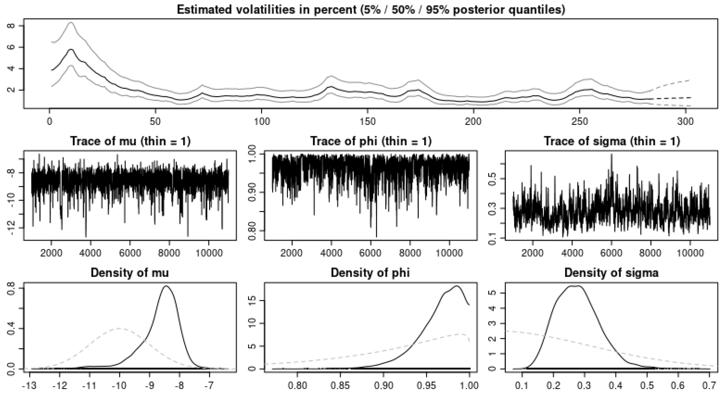
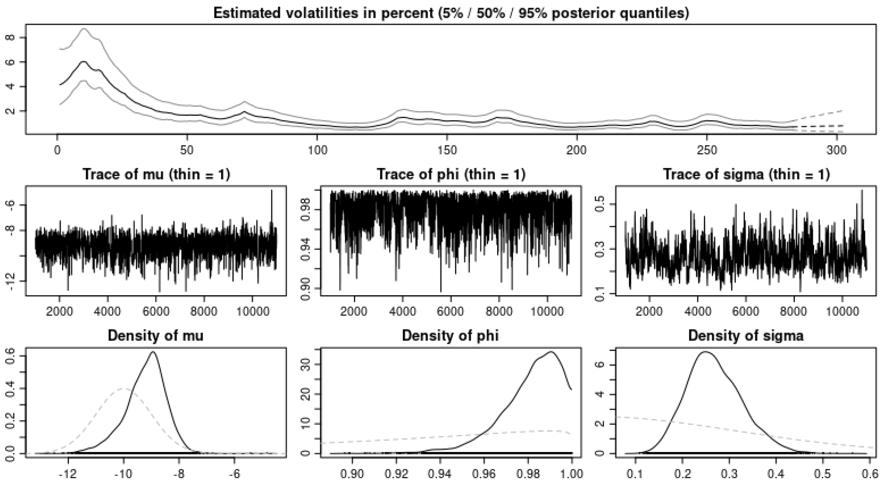
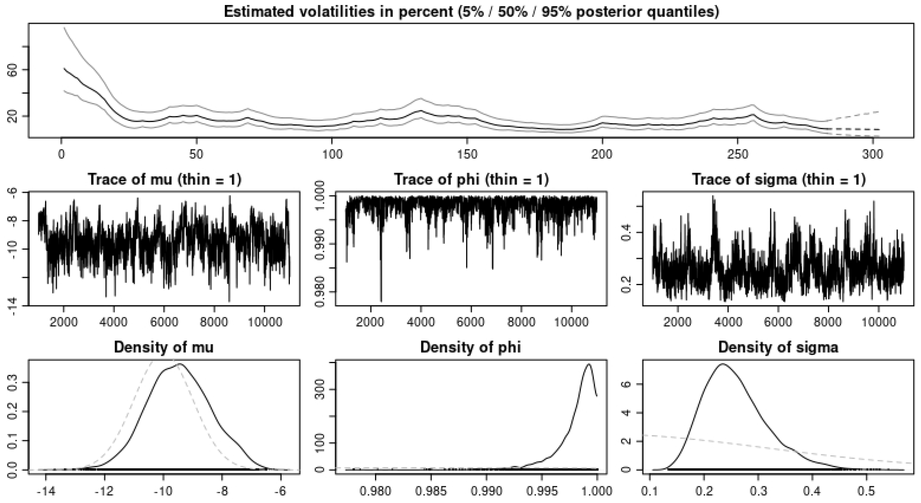
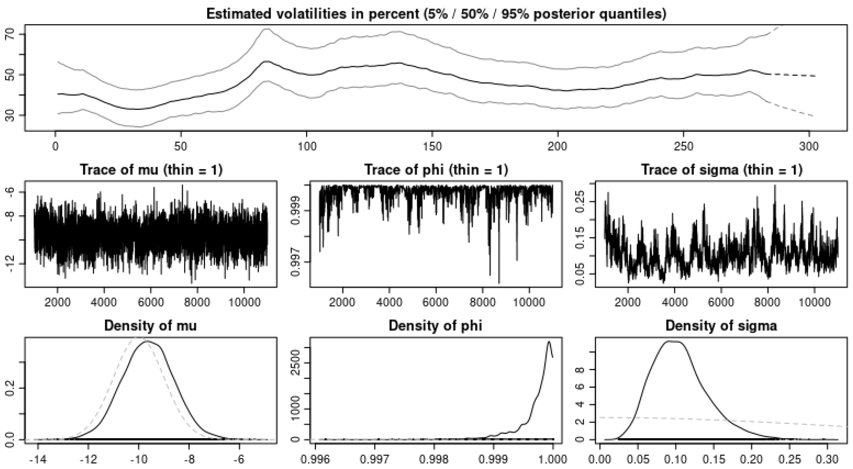
From the model in Section 2, we need to find the parameters and , which are the volatility parameters as well as and , which are the correlation parameters. To estimate these parameters, we make use of the MATLAB and R software. With the MATLAB software, we compute the correlations (see Table 1, Table 2, Table 3 and Table 4) between the data sets, while with the R software, using the astsa and stochvol packages, we estimate the volatilities (see Table 5) within the data at a 95% confidence interval. The results from our estimations are shown in the tables below. We also show that graphs showing the estimated volatilities are also shown in the section.
3.4.2. Volatility Parameter
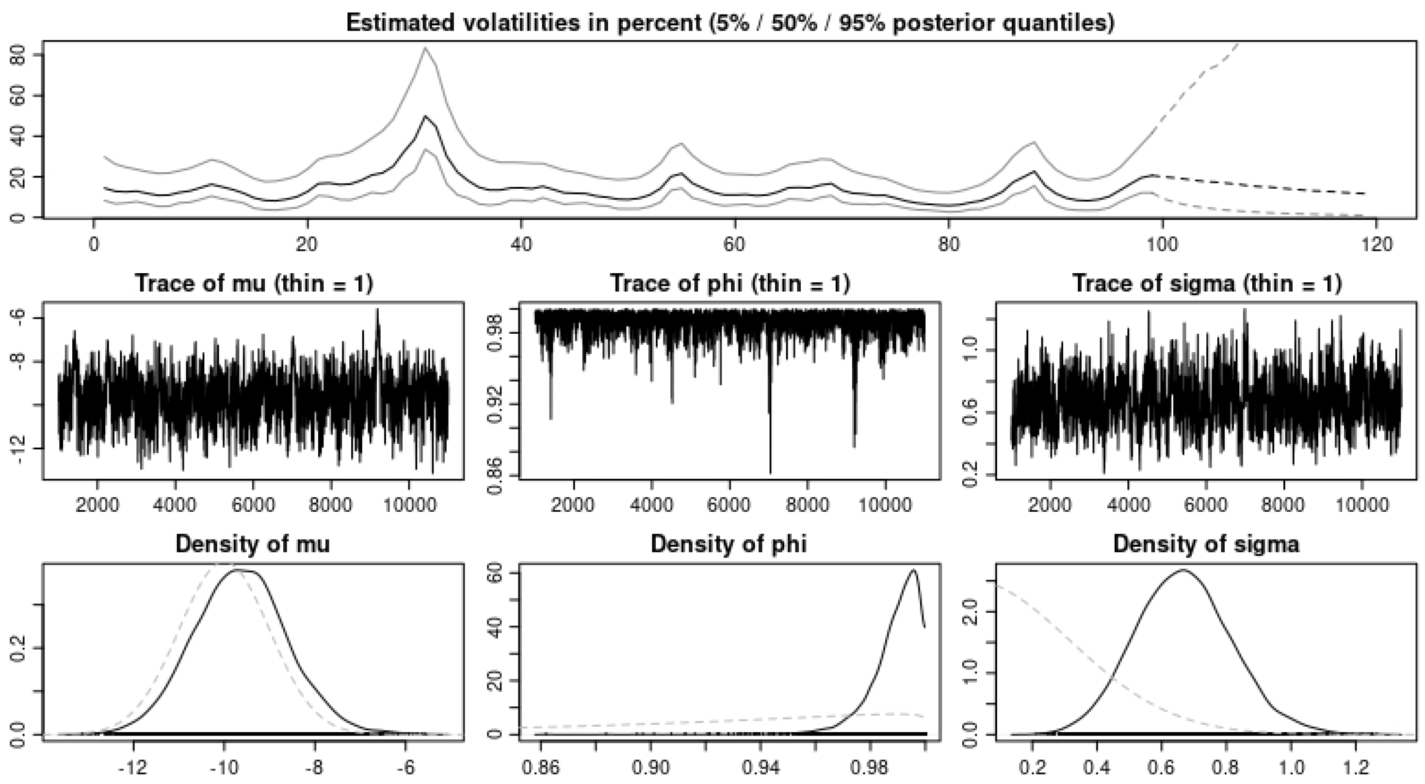
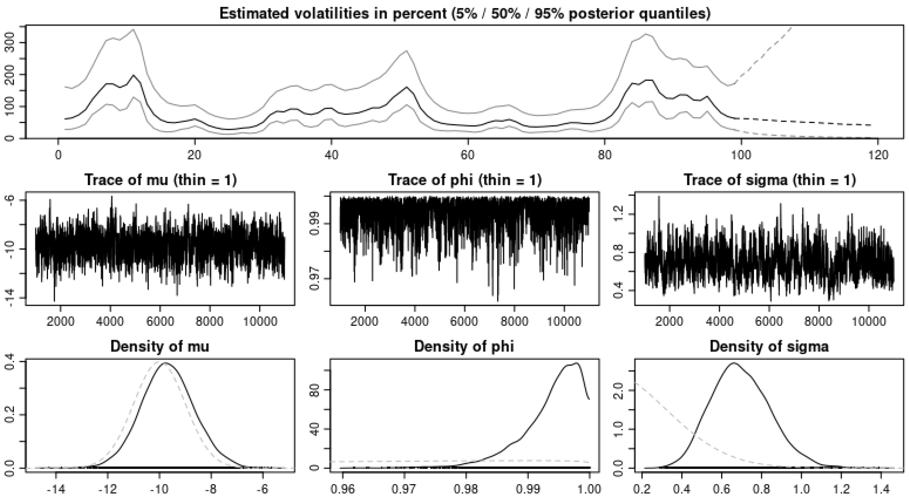
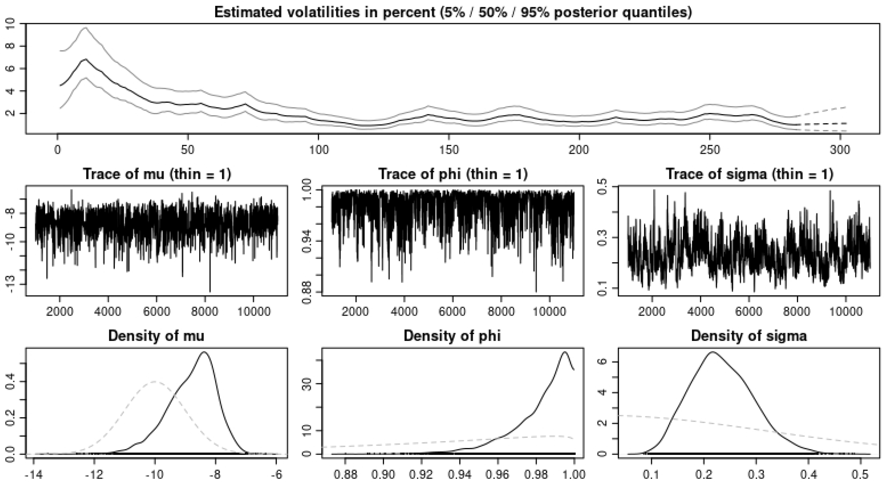
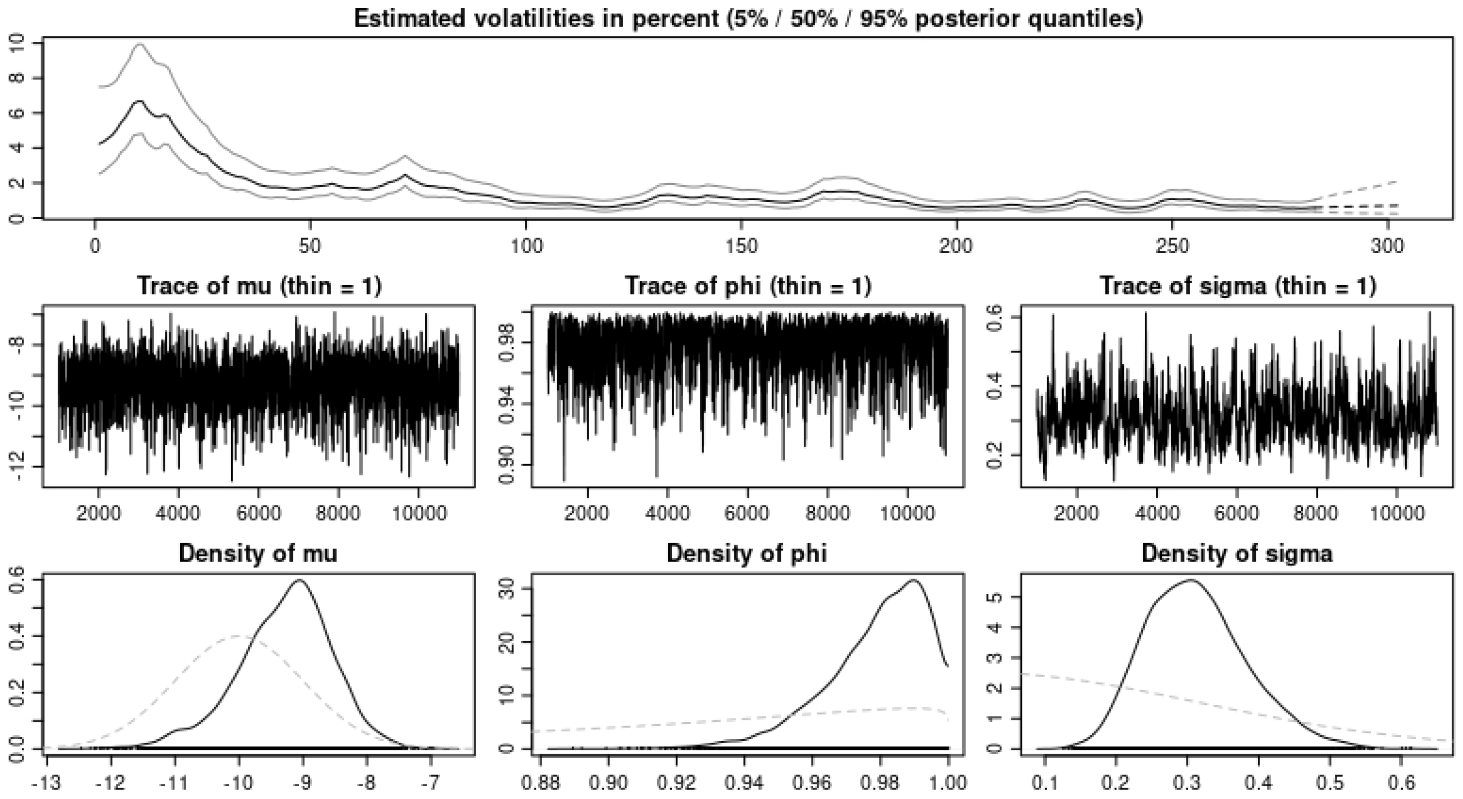
In this section, we show the results obtained for the volatilities using the stockvol package in R [25]. Figure 1, Figure 2, Figure 3, Figure 4, Figure 5, Figure 6, Figure 7 and Figure 8 show the estimated volatilities with a 5%, 50% and 95% posterior quantiles, from which we chose our values from the 95% posterior quantile.
4. Model Applications
This section presents the four different model applications carried out in this work. We present the error estimates when we run predictions with our model on the volcanic eruptions, the financial data, the U.S. COVID-19 data, and a combination of financial data and the U.S. COVID-19 data.
4.1. Error Analysis
In this section, we briefly discuss the errors generated from the model results. Four different error calculations are made to ascertain the accuracy of predictions using the OU system to model multiple data sets. We calculate the root mean squared errors (RMSE), the mean absolute percentage errors (MAPE), the mean absolute errors (MAE), and the average relative percentage errors (ARPE). Formulas used in computing the respective error estimates are explained below. Three sample paths, each with their means, are also graphed below for volcanic eruptions 2 and 8, the NASDAQ and Russell, and the daily U.S. COVID-19 cases and deaths. In addition, six of the data sets are chosen, and three sample paths are graphed for the selected data sets with their means computed and shown on the graphs.
Error Formulas
Suppose y is the true value, p is the predicted value, and n is the number of data points, then we have the following.
Root mean squared error:
Mean absolute percentage error:
Mean absolute error:
Average relative percentage error:
4.2. Application to Volcanic Data
In this section, we present the results obtained from applying our model to volcanic eruptions data. The volcanic eruption data were modeled with both the IG(a,b) coupled OU system and coupled OU system. Three out of the eight eruptions were used for analysis, i.e., eruption 2, eruption 4, and eruption 8. The results are presented in Table 6 and Table 7 for both BDLPs.
4.3. Application to U.S. Stock Markets
In this section, we applied the model to the four main financial portfolios from the U.S. stock market, namely the Dow Jones, the NASDAQ, the S&P500, and the Russell. In the parameter estimations section, we observed that these data sets were highly correlated with correlation coefficients close to 1. Data used were the daily closing values observed from 19 February 2020 to 16 April 2021. We also note that these dates omit the weekends since the stock market is closed during weekends. The results in Table 8 and Table 9 show the error estimates obtained from predictions run using our model with either an IG(a,b) BDLP or a BDLP.
4.4. Application to U.S. COVID-19 Data
In this section, we applied the model to the U.S. COVID-19 data obtained from the New York times between the dates 19 February 2020 and 16 April 2021. We used the model to run predictions on both daily reported cases and daily reported deaths. Results in Table 10 and Table 11 show the error estimates obtained when the BDLP in the model was either a process or an IG(a,b) process.
We observe that the errors from the system of IG(a,b) OU model shown in Table 11 are smaller compared to those of the system of the gamma(a,b) OU model in Table 10. Thus, we obtain lower error estimates from data representing daily U.S. COVID-19 cases and deaths when the BDLP of the coupled OU-system is the inverse Gaussian process.
4.5. Applications to Coupled U.S. COVID-19 and Stock Markets Data
In this section, the system is used to model a combination of stock portfolios and the U.S. COVID-19 data. In the heightened period of the pandemic when infections and death tolls increased, stock prices dropped due to the panic of investors who feared a market crash was imminent. In Section 3, Table 3 and Table 4 show a non-zero correlation between the financial data sets and the daily reported cases and deaths. We model each financial data with the daily reported U.S. COVID-19 cases and the daily reported U.S. COVID-19 deaths. Again, we consider here both BDLPs in order to compare the model performance based on the Lévy process used. Results from the error estimates are shown below in Table 12, Table 13, Table 14 and Table 15.
We observe that the errors from the system of IG(a,b) OU model shown in Table 13 are smaller compared to that of the system of the gamma(a,b) OU model in Table 12. Thus, we obtain lower error estimates from the coupled data from U.S. COVID-19 cases and stock markets when the BDLP of the coupled OU-system is the inverse Gaussian process.
We observe that the errors from the system of IG(a,b) OU model shown in Table 15 are smaller compared to those of the system of the gamma(a,b) OU model in Table 14. Thus, we obtain lower error estimates from the coupled data from U.S. COVID-19 deaths and stock markets when the BDLP of the coupled OU-system is the inverse Gaussian process.
5. Discussion
We ran our model simulation with four different applications and showed that with the data sets modeled, our model prediction gives a good fit for the data sets when we observe the values obtained from the error estimates. In Table 6 and Table 7, we observe an improvement in the MAPE, MAE, and ARPE error estimates with all three eruptions when the BDLP is an IG(a,b) process. However, we observe that the RMSE for eruption 4 with the process gave better results. For the application to the financial data, we observe in Table 8 and Table 9 from the error estimates that for the IG(a,b) as BDLP, our predictions are slightly better compared to those of the . In Table 10 and Table 11, where we model the U.S. COVID-19 cases and deaths, we observe in Table 11 and Table 12 that we obtain the same error estimates with the IG(a,b) and the as BDLPs when we consider the daily cases; however, for the daily deaths, the IG(a,b) BDLP gives a better error estimate. Finally, when we consider Table 12, Table 13, Table 14 and Table 15, we observe good estimates for both IG(a,b) and BDLP when the financial data were modeled with the U.S. COVID-19 cases compared to when they were modeled with the U.S. COVID-19 deaths. This is explained from the strong correlation observed in Table 4 between the financial data and the daily US COVID-19 cases compared to that of the financial data and the daily U.S. COVID-19 deaths. In addition, the three sample paths shown in Figure 9, Figure 10, Figure 11, Figure 12, Figure 13 and Figure 14 for the selected data sets show expected discontinuous paths, making the choice of a Lévy process as the BDP the proper choice. Comparing the sample paths to the original time series, we observe the solution path that best models the data with a mean comparatively closer to that of the time series data. In addition, by modeling the U.S. COVID-19 data using a stochastic SDE, we observe from the three sample paths drawn in Figure 13 and Figure 14 that the disease would potentially die out at some point after it has peaked (both reported cases and deaths) once or multiple times, thus showing that there exist scenarios where the disease will die out.
6. Conclusions
In this work, we applied a coupled system of Ornstein–Uhlenbeck SDEs to various data sets. The results show our model to give good predictions for the data sets under study. With the results from this work, we plan to conduct additional research, using events that may be triggered by a different nearby event. For instance, it is believed that volcanic eruptions can be triggered by nearby earthquakes. We can further research into modeling the system such that and are different Lévy BDPs in order to help improve model predictions since some data sets are best modeled with BDPs while others are best modeled with IG(a,b) BDP.
Author Contributions
Conceptualization, M.C.M., P.K.A., W.K. and O.K.T.; methodology, M.C.M., P.K.A., W.K. and O.K.T.; software, P.K.A.; validation, M.C.M. and O.K.T.; formal analysis, P.K.A.; data curation, P.K.A.; writing—original draft preparation, P.K.A.; writing—review and editing, P.K.A. and O.K.T.; visualization, P.K.A. and W.K.; supervision, M.C.M. and O.K.T. All authors have read and agreed to the published version of the manuscript.
Funding
This research received no external funding.
Institutional Review Board Statement
Not applicable.
Informed Consent Statement
Not applicable.
Data Availability Statement
Data used in this study can be accessed at https://finance.yahoo.com/ (accessed on 21 January 2021) and https://www.nytimes.com/interactive/2020/us/coronavirus-us-cases.html (accessed on 21 January 2021).
Conflicts of Interest
The authors declare no conflict of interest.
Abbreviations
The following abbreviations are used in this manuscript:
| OU | Ornstein–Uhlenbeck |
| BDLP | Background Driving Lévy Process |
| BDP | Background Driving Process |
| RMSE | Root Mean Squared Error |
| MAPE | Mean Absolute Percentage Error |
| MAE | Mean Absolute Error |
| ARPE | Average Relative Percentage Error |
References
- Tian, M.-Y.; Wang, C.-J.; Yang, K.-L.; Fu, P.; Xia, C.-Y.; Zhuo, X.-J.; Wang, L. Estimating the nonlinear effects of an ecological system driven by Ornstein-Uhlenbeck noise. Chaos Solitons Fractals 2020, 136, 109788. [Google Scholar] [CrossRef]
- Caprini, L.; Marconi, U.M.B.; Puglisi, A.; Vulpiani, A. The entropy production of Ornstein–Uhlenbeck active particles: A path integral method for correlations. J. Stat. Mech. Theory Exp. 2019, 2019, 053203. [Google Scholar] [CrossRef] [Green Version]
- Mariani, M.C.; Tweneboah, O.K. Stochastic Differential Equations Applied to the Study of Geophysical and Financial Time Series. Phys. A 2016, 443, 170–178. [Google Scholar] [CrossRef]
- Janczura, J.; Orzeł, S.; Wyłomańska, A. Subordinated α-stable Ornstein–Uhlenbeck process as a tool for financial data description. Phys. A Stat. Mech. Its Appl. 2011, 390, 4379–4387. [Google Scholar] [CrossRef]
- Mariani, M.; Tweneboah, O.K. Modeling high frequency stock market data by using stochastic models. Stoch. Anal. Appl. 2021. [Google Scholar] [CrossRef]
- Barndorff-Nielsen, O.E.; Shephard, N. Non-Gaussian Ornstein–Uhlenbeck-based models and some of their uses in financial economics. J. R. Stat. Soc. Ser. B Stat. Methodol. 2001, 63, 167–241. [Google Scholar] [CrossRef]
- Obuchowski, J.; Wylomanska, A. Ornstein-Uhlenbeck Process with Non-Gaussian Structure. Acta Phys. Pol. 2013, 44, 1123–1133. [Google Scholar] [CrossRef] [Green Version]
- Maller, R.A.; Müller, G.; Szimayer, A. Ornstein-Uhlehnbeck Process and Extensions. Handb. Financ. Time Ser. 2009, 421–437. [Google Scholar]
- Eliazar, I.; Klafter, J. Lévy, Ornstein–Uhlenbeck, and subordination: Spectral vs. jump description. J. Stat. Phys. 2005, 119, 165–196. [Google Scholar] [CrossRef]
- Mariani, M.C.; Asante, P.K.; Bhuiyan, M.A.M.; Beccar-Varela, M.P.; Jaroszewicz, S.; Tweneboah, O.K. Long-Range Correlations and Characterization of Financial and Volcanic Time Series. Mathematics 2020, 8, 441. [Google Scholar] [CrossRef] [Green Version]
- Endres, S.; Stübinger, J. Optimal trading strategies for Lévy-driven Ornstein–Uhlenbeck processes. Appl. Econ. 2019, 51, 3153–3169. [Google Scholar] [CrossRef]
- Available online: https://www.adn.com/science/article/alaskas-biggest-volcanic-eruptions/2012/02/28/ (accessed on 5 January 2021).
- Voight, B. A method for prediction of volcanic eruptions. Nature 1988, 332, 125–130. [Google Scholar] [CrossRef]
- Robock, A. Volcanic eruptions and climate. Rev. Geophys. 2000, 38, 191–219. [Google Scholar] [CrossRef]
- Linde, A.T.; Sacks, I.S. Triggering of volcanic eruptions. Nature 1998, 395, 888–890. [Google Scholar] [CrossRef]
- Sparks, R.; Steve, J. Forecasting volcanic eruptions. Earth Planet. Sci. Lett. 2003, 210, 1–15. [Google Scholar] [CrossRef]
- Brenguier, F.; Shapiro, N.M.; Campillo, M.; Ferrazzini, V.; Duputel, Z.; Coutant, O.; Nercessian, A. Towards forecasting volcanic eruptions using seismic noise. Nat. Geosci. 2008, 1, 126–130. [Google Scholar] [CrossRef] [Green Version]
- Abadie, L.M. Current expectations and actual values for the clean spark spread: The case of Spain in the Covid-19 crisis. J. Clean. Prod. 2021, 285, 124842. [Google Scholar] [CrossRef]
- Mandal, M.; Jana, S.; Nandi, S.K.; Khatua, A.; Adak, S.; Kar, T.K. A model based study on the dynamics of COVID-19: Prediction and control. Chaos Solitons Fractals 2020, 136, 109889. [Google Scholar] [CrossRef]
- Calafiore, G.C.; Novara, C.; Possieri, C. A time-varying SIRD model for the COVID-19 contagion in Italy. Annu. Rev. Control. 2020, 50, 361–372. [Google Scholar] [CrossRef]
- IHME COVID-19 Forecasting Team. Modeling COVID-19 scenarios for the United States. Nat. Med. 2021, 27, 94. [Google Scholar] [CrossRef]
- Habtemicael, S.; SenGupta, I. Ornstein–Uhlenbeck processes for geophysical data analysis. Phys. A Stat. Mech. Its Appl. 2014, 399, 147–156. [Google Scholar] [CrossRef]
- Oravecz, Z.; Tuerlinckx, F.; Vandekerckhove, J. Bayesian data analysis with the bivariate hierarchical Ornstein-Uhlenbeck process model. Multivar. Behav. Res. 2016, 51, 106–119. [Google Scholar] [CrossRef] [PubMed] [Green Version]
- Oravecz, Z.; Tuerlinckx, F.; Vandekerckhove, J. A hierarchical Ornstein–Uhlenbeck model for continuous repeated measurement data. Psychometrika 2009, 74, 395–418. [Google Scholar] [CrossRef]
- Kastner, G. Dealing with stochastic volatility in time series using the R package stochvol. arXiv 2019, arXiv:1906.12134. [Google Scholar]
- Helbing, D.; Brockmann, D.; Chadefaux, T.; Donnay, K.; Blanke, U.; Woolley-Meza, O.; Moussaid, M.; Johansson, A.; Krause, J.; Schutte, S.; et al. Saving human lives: What complexity science and information systems can contribute. J. Stat. Phys. 2015, 158, 735–781. [Google Scholar] [CrossRef] [PubMed]
- Available online: https://www.nytimes.com/interactive/2020/us/coronavirus-us-cases.html (accessed on 21 January 2021).
Figure 1.
Graph showing estimated volatility for eruption 2.

Figure 2.
Graph showing estimated volatility for eruption 4.

Figure 3.
Graph showing estimated volatility for the Russell.

Figure 4.
Graph showing estimated volatility for the Dow Jones.

Figure 5.
Graph showing estimated volatility for the NASDAQ.

Figure 6.
Graph showing estimated volatility for the S&P500.

Figure 7.
Graph showing estimated volatility for U.S. COVID-19 cases.

Figure 8.
Graph showing estimated volatility for U.S. COVID-19 deaths.

Figure 9.
Graph showing three sample paths and time series plot for eruption 2. We observe from the sample paths that sample path 3 closely predicts the time series and see by comparison of the means that sample path 3 is closer in value to the mean of the time series data.
Figure 9.
Graph showing three sample paths and time series plot for eruption 2. We observe from the sample paths that sample path 3 closely predicts the time series and see by comparison of the means that sample path 3 is closer in value to the mean of the time series data.

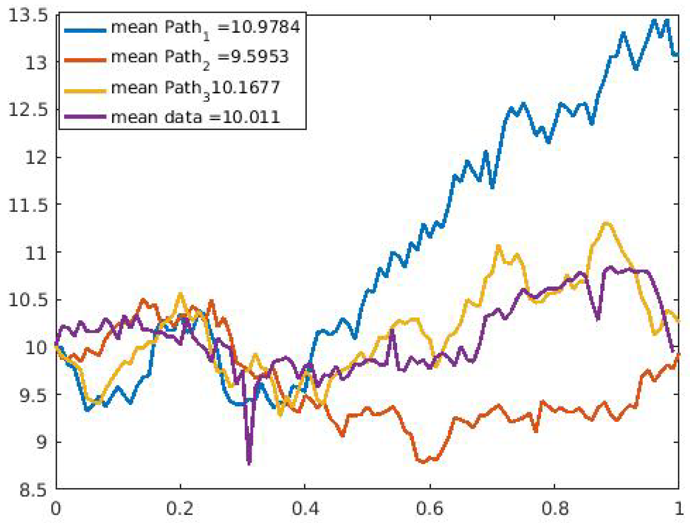
Figure 10.
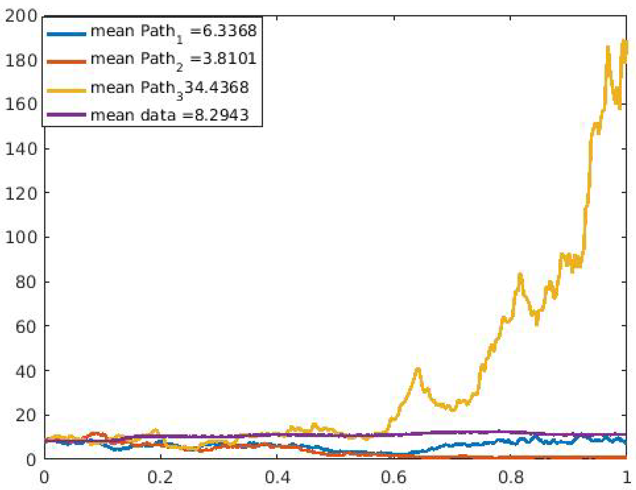
Graph showing three sample paths and time series plot for eruption 8. We notice that eruption 8 has 2 extreme values, which may affect the model’s performance. For this time series, we again see that sample path 3 closely predicts it and by comparison of the means, sample path 3 is closer in value to the mean of the time series data.
Figure 10.
Graph showing three sample paths and time series plot for eruption 8. We notice that eruption 8 has 2 extreme values, which may affect the model’s performance. For this time series, we again see that sample path 3 closely predicts it and by comparison of the means, sample path 3 is closer in value to the mean of the time series data.

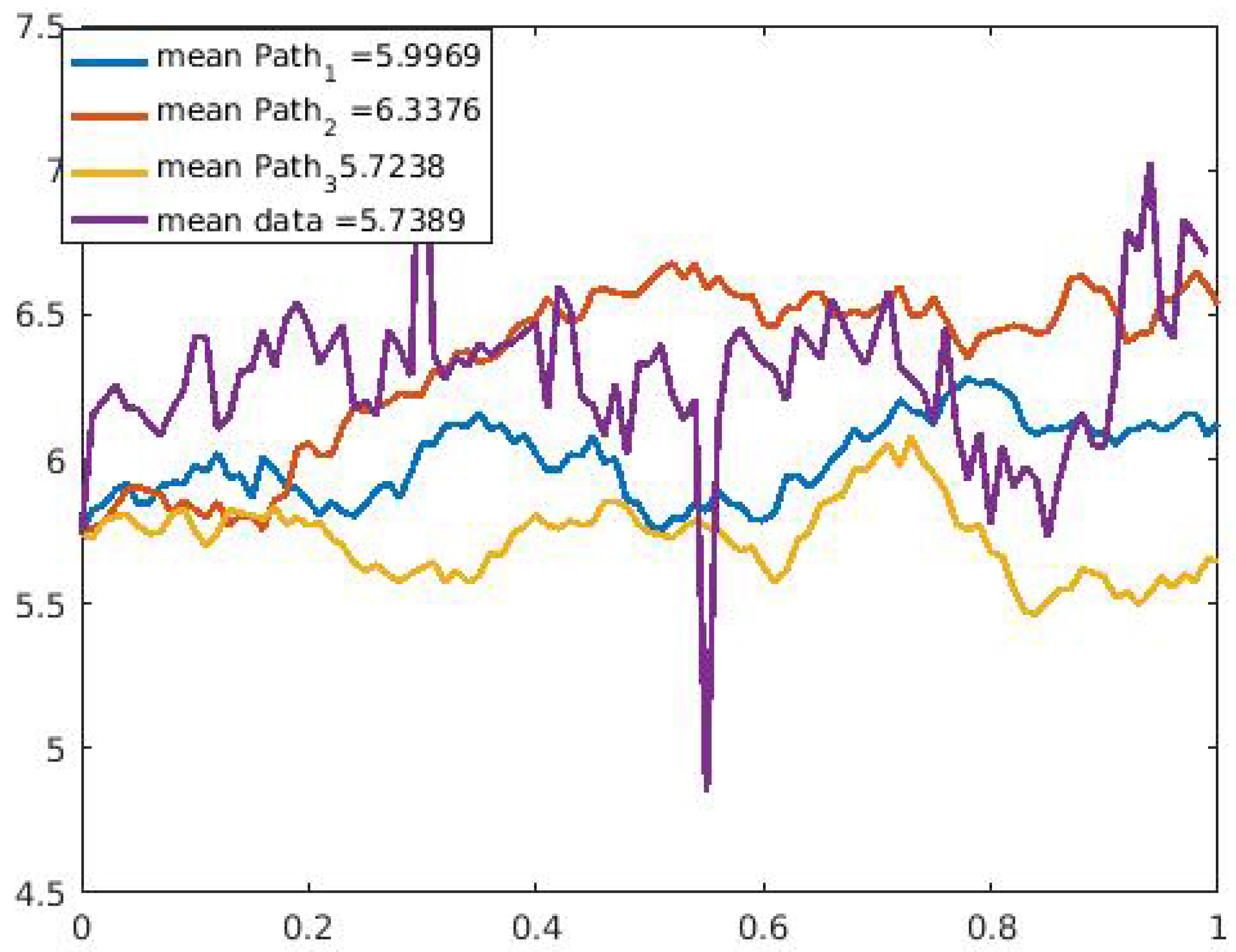
Figure 11.
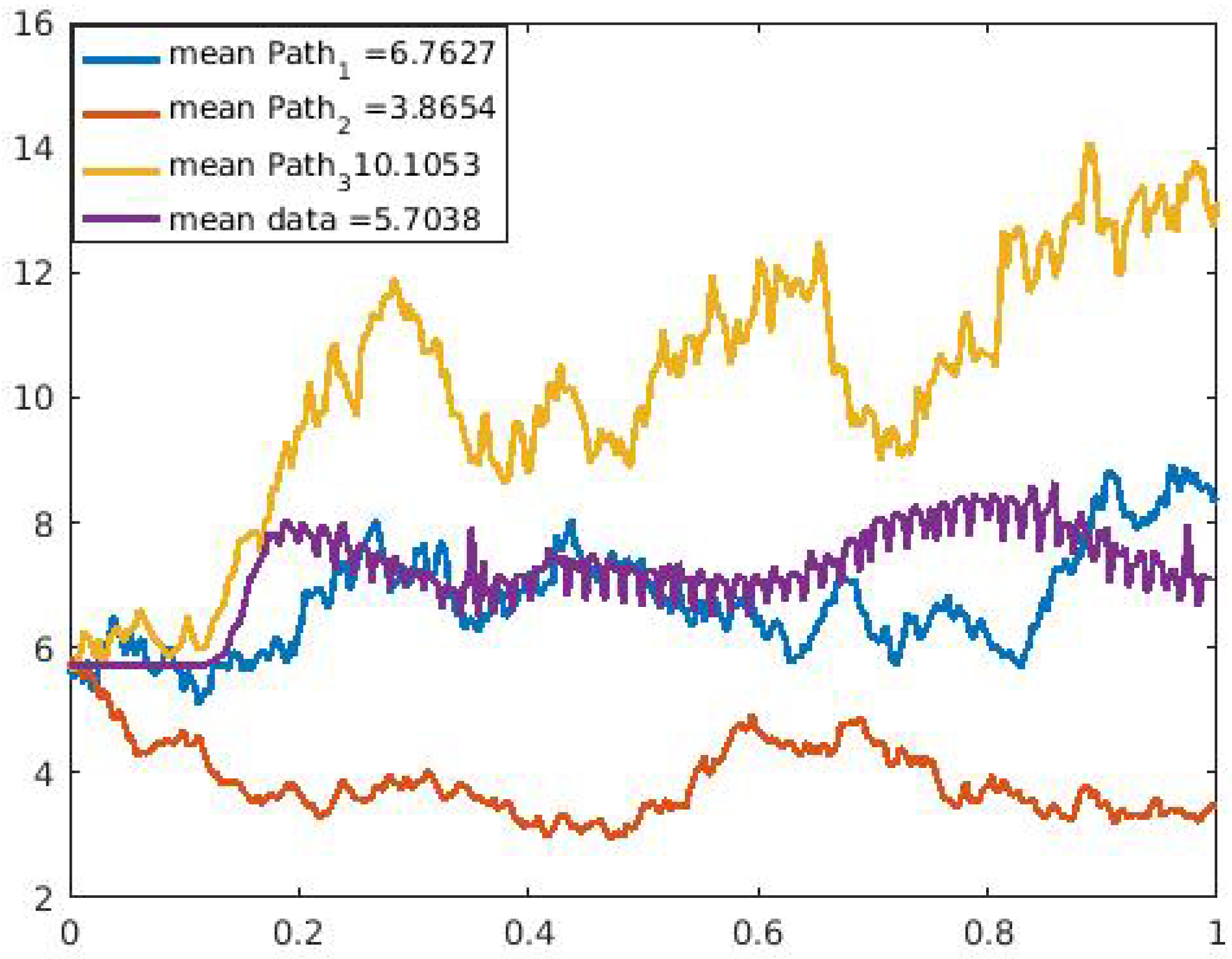
Graph showing three sample paths and time series plot for the Russell index. For this time series, we see that sample path 2 closely predicts it and by comparison of the means, sample path 2 is closer in value to the mean of the time series data.
Figure 11.
Graph showing three sample paths and time series plot for the Russell index. For this time series, we see that sample path 2 closely predicts it and by comparison of the means, sample path 2 is closer in value to the mean of the time series data.

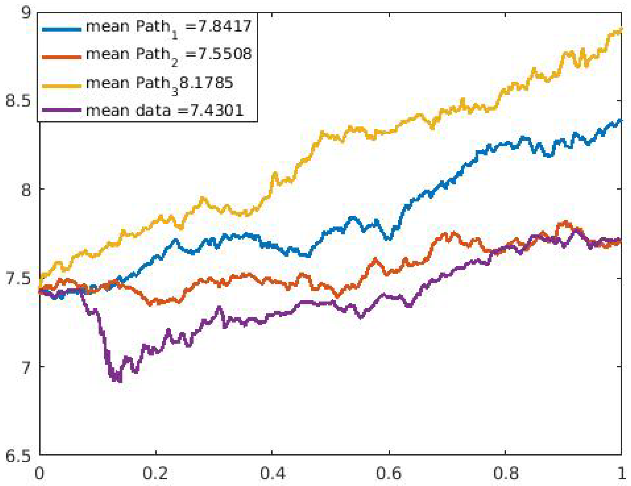
Figure 12.
Graph showing three sample paths and time series plot for the NASDAQ index. For this time series, we see that sample path 2 closely predicts it and by comparison of the means, sample path 2 is closer in value to the mean of the time series data.
Figure 12.
Graph showing three sample paths and time series plot for the NASDAQ index. For this time series, we see that sample path 2 closely predicts it and by comparison of the means, sample path 2 is closer in value to the mean of the time series data.

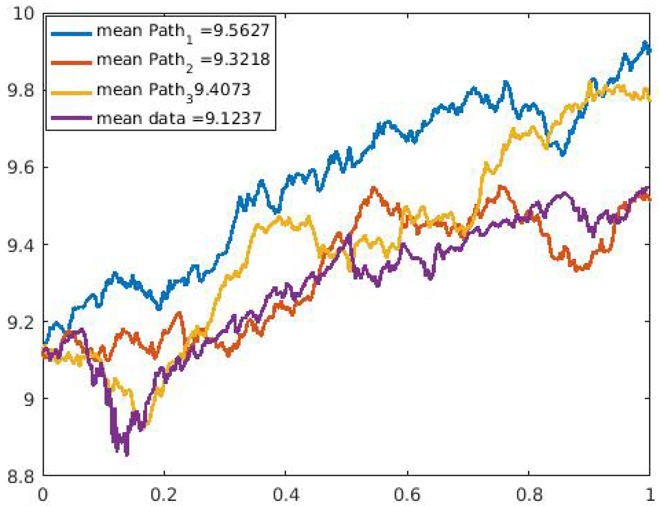
Figure 13.
Graph showing three sample paths and time series plot for the U.S. COVID-19 cases. For this time series, we see that sample path 1 closely predicts it and by comparison of the means, sample path 1 is closer in value to the mean of the time series data.
Figure 13.
Graph showing three sample paths and time series plot for the U.S. COVID-19 cases. For this time series, we see that sample path 1 closely predicts it and by comparison of the means, sample path 1 is closer in value to the mean of the time series data.

Figure 14.
Graph showing three sample paths and time series plot for the U.S. COVID-19 deaths. For this time series, we see that sample path 1 closely predicts it and by comparison of the means, sample path 1 is closer in value to the mean of the time series data.
Figure 14.
Graph showing three sample paths and time series plot for the U.S. COVID-19 deaths. For this time series, we see that sample path 1 closely predicts it and by comparison of the means, sample path 1 is closer in value to the mean of the time series data.


Table 1.
Correlation matrix for volcanic eruptions.
| Eruption 2 | Eruption 4 | Eruption 8 | |
|---|---|---|---|
| Eruption 2 | 1 | 0.0626 | −0.0754 |
| Eruption 4 | 0.0626 | 1 | 0.0127 |
| Eruption 8 | −0.0754 | 0.0127 | 1 |
Table 2.
Correlation matrix for stock markets.
| Stock Markets | Dow Jones | S&P500 | NASDAQ | Russell |
|---|---|---|---|---|
| Dow Jones | 1 | 0.9942 | 0.9618 | 0.9590 |
| S&P500 | 0.9942 | 1 | 0.9840 | 0.9596 |
| NASDAQ | 0.9618 | 0.9840 | 1 | 0.9258 |
| Russell | 0.9590 | 0.9596 | 0.9258 | 1 |
Table 3.
Correlation matrix U.S.A. COVID-19 cases and deaths.
| U.S.A. COVID-19 Cases | U.S.A. COVID-19 Deaths | |
|---|---|---|
| USA COVID-19 Cases | 1 | 0.6755 |
| USA COVID-19 Deaths | 0.6755 | 1 |
Table 4.
Correlation matrix for stock markets and U.S.A. COVID-19 cases and deaths.
| Stock Markets | U.S.A. COVID-19 Cases | U.S.A. COVID-19 Deaths |
|---|---|---|
| Dow Jones | 0.5576 | 0.3829 |
| S&P500 | 0.5861 | 0.4202 |
| NASDAQ | 0.6219 | 0.4539 |
| Russell | 0.5741 | 0.4858 |
Table 5.
lVolatility Values Estimated Using R stochvol package.
| Data | Volatility () |
|---|---|
| Dow Jones | −5.123718 |
| S&P500 | −5.255099 |
| NASDAQ | −5.444095 |
| Russell | −5.120774 |
| Eruption 2 | −7.906 |
| Eruption 4 | −7.967 |
| Eruption 8 | −7.84 |
| U.S.A. COVID-19 Cases | 0.006128 |
| U.S.A. COVID-19 Deaths | −1.116847 |
Table 6.
Results from system of gamma(a,b) OU model. The results reported are the best results from modeling a combination of eruptions 2, eruptions 4 and eruptions 8.
Table 6.
Results from system of gamma(a,b) OU model. The results reported are the best results from modeling a combination of eruptions 2, eruptions 4 and eruptions 8.
| Eruptions | RMSE | MAPE | MAE | ARPE |
|---|---|---|---|---|
| Eruption 2 | 0.7654 | 0.0049 | 34,685.5 | 1.3275 |
| Eruption 4 | 1.3218 | 6.5506 | 156.69 | 13.33 |
| Eruption 8 | 0.8088 | 0.8212 | 2419.4 | 4.6206 |
Table 7.
Results from system of IG(a,b) OU model. The results reported are the best results from modeling a combination of eruptions 2, eruptions 4 and eruptions 8.
Table 7.
Results from system of IG(a,b) OU model. The results reported are the best results from modeling a combination of eruptions 2, eruptions 4 and eruptions 8.
| Eruptions | RMSE | MAPE | MAE | ARPE |
|---|---|---|---|---|
| Eruption 2 | 0.3927 | 0.0013 | 8518.93 | 0.3411 |
| Eruption 4 | 1.8168 | 4.547 | 18.597 | 0.926 |
| Eruption 8 | 0.5839 | 0.0646 | 216.49 | 0.3633 |
Table 8.
Results from system of OU model. The results reported are the best results from modeling a combination of the Dow Jones, the S&P500, the NASDAQ and the Russell.
Table 8.
Results from system of OU model. The results reported are the best results from modeling a combination of the Dow Jones, the S&P500, the NASDAQ and the Russell.
| Stock Markets | RMSE | MAPE | MAE | ARPE |
|---|---|---|---|---|
| Dow Jones | 0.1798 | 0.0014 | 3950.69 | 0.1385 |
| S&P500 | 0.1574 | 0.0111 | 446.16 | 0.1318 |
| NASDAQ | 0.2428 | 0.0046 | 2009.52 | 0.1838 |
| Russell | 0.2219 | 0.0338 | 320.85 | 0.1992 |
Table 9.
Results from system of IG(a,b) OU model. The results reported are the best results from modeling a combination of the Dow Jones, the S&P500, the NASDAQ and the Russell.
Table 9.
Results from system of IG(a,b) OU model. The results reported are the best results from modeling a combination of the Dow Jones, the S&P500, the NASDAQ and the Russell.
| Stock Markets | RMSE | MAPE | MAE | ARPE |
|---|---|---|---|---|
| Dow Jones | 0.1259 | 0.001 | 2773.07 | 0.1027 |
| S&P500 | 0.1360 | 0.0095 | 365.58 | 0.1125 |
| NASDAQ | 0.1762 | 0.0038 | 1547.44 | 0.1495 |
| Russell | 0.2235 | 0.0334 | 319.25 | 0.1967 |
Table 10.
Results from system of OU model.
| U.S. COVID-19 Data | RMSE | MAPE | MAE | ARPE |
|---|---|---|---|---|
| Daily Cases | 1.648 | 0.3874 | 51,573.23 | 106.74 |
| Daily Deaths | 3.1713 | 7.5384 | 28,204.32 | 40.40 |
Table 11.
Results from system of IG(a,b) OU model.
| U.S. COVID-19 Data | RMSE | MAPE | MAE | ARPE |
|---|---|---|---|---|
| Daily Cases | 1.648 | 0.3874 | 51,573.23 | 106.74 |
| Daily Deaths | 1.4193 | 3.1076 | 828.20 | 16.65 |
Table 12.
Results from system of OU model. The results reported are the best results from modeling a combination of U.S.A. COVID-19 cases with the stock market data.
Table 12.
Results from system of OU model. The results reported are the best results from modeling a combination of U.S.A. COVID-19 cases with the stock market data.
| Data | RMSE | MAPE | MAE | ARPE |
|---|---|---|---|---|
| Daily Cases | 1.6481 | 0.3874 | 51,525.03 | 106.74 |
| Dow Jones | 0.2684 | 0.0027 | 6071.4 | 0.2052 |
| S&P500 | 0.5678 | 0.0631 | 2516.53 | 0.7486 |
| NASDAQ | 0.182 | 0.0041 | 1551.14 | 0.1598 |
| Russell | 0.5211 | 0.1057 | 1133.73 | 0.6226 |
Table 13.
Results from system of IG(a,b) OU model. The results reported are the best results from modeling a combination of U.S.A. COVID-19 cases with the stock market data.
Table 13.
Results from system of IG(a,b) OU model. The results reported are the best results from modeling a combination of U.S.A. COVID-19 cases with the stock market data.
| Data | RMSE | MAPE | MAE | ARPE |
|---|---|---|---|---|
| Daily Cases | 1.6481 | 0.3874 | 51,530.41 | 106.74 |
| Dow Jones | 0.1259 | 0.0015 | 2773.07 | 0.1027 |
| S&P500 | 0.136 | 0.0095 | 365.56 | 0.1125 |
| NASDAQ | 0.1762 | 0.0038 | 1547.44 | 0.1495 |
| Russell | 0.2235 | 0.0334 | 319.25 | 0.1967 |
Table 14.
Results from system of OU model. The results reported are the best results from modeling a combination of U.S.A. COVID-19 deaths with the stock market data.
Table 14.
Results from system of OU model. The results reported are the best results from modeling a combination of U.S.A. COVID-19 deaths with the stock market data.
| Data | RMSE | MAPE | MAE | ARPE |
|---|---|---|---|---|
| Daily Deaths | 1.4192 | 3.1049 | 823.32 | 16.64 |
| Dow Jones | 0.1820 | 0.0014 | 4002.92 | 0.14 |
| S&P500 | 0.1612 | 0.0011 | 456.29 | 0.1347 |
| NASDAQ | 0.267 | 0.0058 | 2535.05 | 0.2263 |
| Russell | 0.389 | 0.0537 | 537.49 | 0.3092 |
Table 15.
Results from system of IG(a,b) OU model. The results reported are the best results from modeling a combination of U.S.A. COVID-19 deaths with the stock market data.
Table 15.
Results from system of IG(a,b) OU model. The results reported are the best results from modeling a combination of U.S.A. COVID-19 deaths with the stock market data.
| Data | RMSE | MAPE | MAE | ARPE |
|---|---|---|---|---|
| Daily Deaths | 1.4192 | 3.1076 | 828.20 | 16.65 |
| Dow Jones | 0.1259 | 0.0010 | 2773.07 | 0.103 |
| S&P500 | 0.136 | 0.0095 | 365.58 | 0.1125 |
| NASDAQ | 0.1762 | 0.0038 | 1547.44 | 0.1495 |
| Russell | 0.2235 | 0.0334 | 319.25 | 0.1967 |
Publisher’s Note: MDPI stays neutral with regard to jurisdictional claims in published maps and institutional affiliations. |
© 2022 by the authors. Licensee MDPI, Basel, Switzerland. This article is an open access article distributed under the terms and conditions of the Creative Commons Attribution (CC BY) license (https://creativecommons.org/licenses/by/4.0/).
Share and Cite
MDPI and ACS Style
Mariani, M.C.; Asante, P.K.; Kubin, W.; Tweneboah, O.K. Data Analysis Using a Coupled System of Ornstein–Uhlenbeck Equations Driven by Lévy Processes. Axioms 2022, 11, 160. https://doi.org/10.3390/axioms11040160
AMA Style
Mariani MC, Asante PK, Kubin W, Tweneboah OK. Data Analysis Using a Coupled System of Ornstein–Uhlenbeck Equations Driven by Lévy Processes. Axioms. 2022; 11(4):160. https://doi.org/10.3390/axioms11040160
Chicago/Turabian StyleMariani, Maria C., Peter K. Asante, William Kubin, and Osei K. Tweneboah. 2022. "Data Analysis Using a Coupled System of Ornstein–Uhlenbeck Equations Driven by Lévy Processes" Axioms 11, no. 4: 160. https://doi.org/10.3390/axioms11040160
Note that from the first issue of 2016, this journal uses article numbers instead of page numbers. See further details here.