Generalization of Fuzzy Connectives

Abstract

This paper is centered around the creation of new fuzzy connectives using automorphism functions. The fuzzy connectives theory has been implemented in many problems and fields. In particular, the N-negations, t-norms, S-conorms and I-implications concepts played crucial roles in forming the theory and applications of the fuzzy sets. Thus far, there are multiple strategies for producing fuzzy connectives. The purpose of this paper is to provide a new strategy that is more flexible and fast in comparison with the rest. In order to create this method, automorphism and additive generator functions were utilized. The general formulas created with this method can provide new fuzzy connectives. The main conclusion is that new fuzzy connectives can be created faster and with more flexibility with our strategy.

1. Introduction

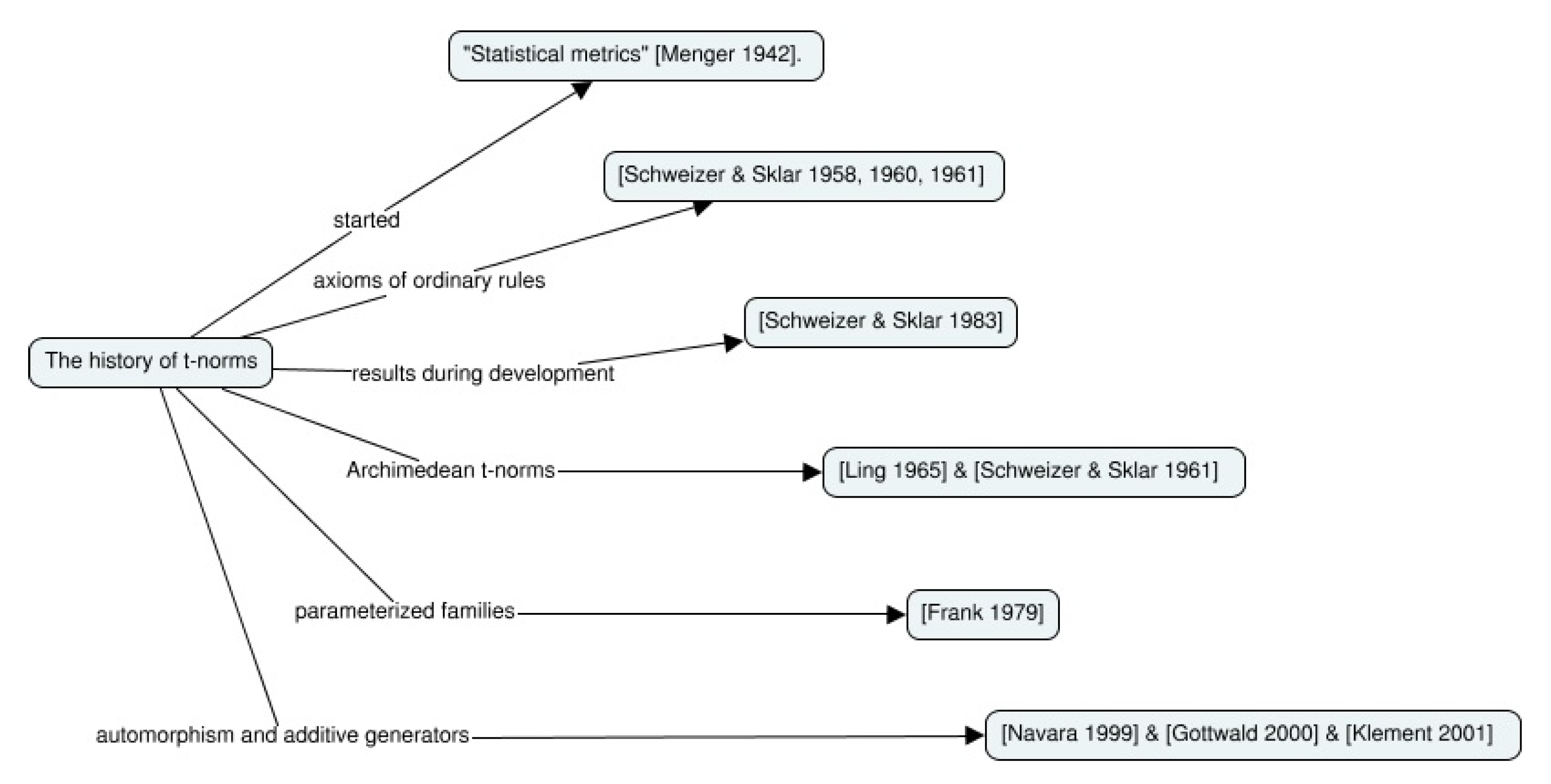
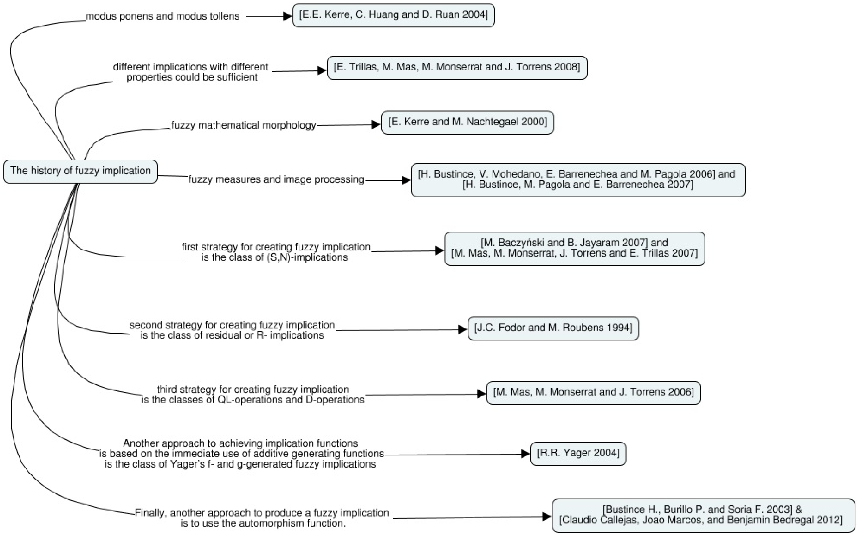
Fuzzy connectives play a crucial role in many applications of fuzzy logic, such as approximate reasoning, formal methods of proof, inference systems, and decision support systems. Recognizing the above importance, many methods of creating fuzzy connectives have been discovered. Most of them refer to the t-norms and I-implications fuzzy connectives. These methods, as well as the fuzzy connectives they produce, are visible in Figure 1.

In 1942, Menger, in his paper “Statistical metrics”, was the first to use the concept of t-norms [1]. Schweizer B. and Sklar A., in work published in 1958, 1960, 1961 and 1983 [2], defined the axioms of ordinary rules and presented the results that occurred during development. Then, Ling C.H., in 1965 [3], built upon B. Schweizer’s and A. Sklar’s work and defined the Archimedean t-norms. Frank M.J., in 1979 [4], defined the parameterized families of t-norms. Finally, Navara M. in 1999 [5], Gottwald S. in 2000 [6] and Klement E.P. in 2001 [7] introduced the method of producing t-norms via automorphism and additive generator functions.

Kerre E., Huang C. and Ruan D. discovered the modus ponens and modus tollens in 2004 [8]; Trillas E., Mas M., Monserrat M. and Torrens J., in 2008, discovered different implications with varying properties [9]. Thereafter, in 2004, Kerre E. and Nachtegael M. formed the fuzzy mathematical morphology [10]. Furthermore, Bustince H. et al., in 2006, discovered fuzzy measures and image processing [11]. Moreover, Baczyński M. and Jayaram B., as well as Mas M., Monserrat M., Torrens J. and Trillas E., in 2007, created the first strategy, which generates (S,N)-implications [12,13]; Fodor J.C. and Roubens M., in 1994, created the second strategy, which generates R-Implications [14]. The third strategy, which generates QL and D-operations, was created by Mas M., Monserrat M. and Torrens J. in 2006 [15]. In 2004, Yager R.R. created the fourth strategy, which generates f- and g-implications [16]. Finally, Bustince H., Burillo P. and Soria F. in 2003 [17], as well as Callejas C., Marcos J. and Bedregal B. in 2012, created the fifth strategy, which generates any fuzzy implication [18].

Since 2012, there has been no further research focused on the fuzzy connectives. Therefore, this paper was created in order to build upon the previous discoveries and improve them by creating a faster and more flexible strategy for producing fuzzy connectives, which, in turn, produces more flexible results.

2. Literature Review

In the Introduction, a review of milestones achieved by other researchers in the field of fuzzy connectives was given. However, this section is dedicated to the presentation of published research of other researchers in the field of the generalization of fuzzy connectives. The goal of this presentation is the exploration of other viewpoints on the subject of this paper. In the following table, the research published for every primary category of fuzzy connectives is presented:

The field of the generalization of fuzzy connectives has been explored by many researchers over the years. As a result, the four main categories of fuzzy connectives have been the subject of many research papers which contributed to the development of the field.

The published research of the negation connectives category (see

Table 1. Published research of every fuzzy connectives category.

Category	Published Research
Negation Connectives	Fuzzy Preference Modelling and
	Multicriteria Decision Support [14]
	“Nilpotent Minimum and
	Related Connectives for Fuzzy Logics” [19]
	“A treatise on many-valued logics” [6]
Conjunction Connectives	“A treatise on many-valued logics” [6]
	“Triangular norms” [7]
	“Characterization of Measures Based
	on Strict Triangular Norms” [5]
	“The best interval representations
	of t-norms and automorphisms” [20]
Disjunction Connectives	“Connectives in Fuzzy Logic” [21]
	Fuzzy Implications [22]
	“A treatise on many-valued logics” [6]
	“Triangular norms” [7]
Implication Connectives	“Fuzzy Implications” [22]
	“Automorphisms, negations and
	implication operators” [17]
	“Actions of Automorphisms on Some Classes
	of Fuzzy Bi-implications” [18]

) offered many contributions to the field of the generalization of fuzzy connectives. To be more specific, the book Fuzzy Preference Modelling and Multicriteria Decision Support (see [14]) and paper “Related Connectives for Fuzzy Logics” (see [19]) contributed by offering definitions, properties and theorems. The paper “A treatise on many-valued logics” (see [6]) contributed by offering a new strategy for generalizing fuzzy connectives via automorphisms.

Similarly, for the conjunction connectives: The paper “A Treatise on Many-Valued Logics” (see [6]) contributed by offering new methods for generalizing conjunction connectives. The paper “Triangular norms” (see [7]) contributed by offering new methods for constructing t-norms as well as t-norm families. The paper “Characterization of Measures Based on Strict Triangular Norms” (see [5]) contributed by offering new strategies for producing t-norms and especially Frank’s t-norms. The paper “The best interval representations of t-norms and automorphisms” (see [20]) contributed by offering new methods of producing t-norms, especially interval t-norms and interval automorphisms.

Similarly, for the disjunction connectives: The paper “Connectives in Fuzzy Logic” (see [21]) contributed by offering new triples of t-norms, t-conorms and n-negations, which prove multiple theorems. The book Fuzzy Implications (see [22]) contributed by offering a complete presentation of the published research until 2008. The paper “A treatise on many-valued logics” (see [6]) contributed by offering a combination of t-norms and t-conorms, which proves multiple theorems. The paper “Triangular norms” (see [7]) contributed by offering a combination of t-norms and t-conorms, which proves multiple definitions and properties.

Finally, for the implication connectives: The book Fuzzy Implications (see [22]) contributed by offering a complete presentation of the published research until 2008. The paper “Automorphisms, negations and implication operators” (see [17]) contributed by offering a new strategy for constructing implications via automorphisms. The paper “Actions of Automorphisms on Some Classes of Fuzzy Bi-implications” (see [18]) contributed by offering a new class of implications, using automorphisms, the bi-implications class.

3. Preliminaries

In this section, the definitions and basic properties of the negation, conjunction, disjunction and implication operators in fuzzy logic are provided. The concepts of automorphism and conjugate are used throughout the whole paper.

3.1. Fuzzy Negations

Some definitions retrieved from the literature can be found in the following references: (Baczyński M., 1.4.1–1.4.2 Definitions, pp. 13–14, [22]), (Bedregal B.C., p. 1126, [23]), (Fodor J., 1.1–1.2 Definitions, p. 3, [14]), (Gottwald S., 5.2.1 Definition, p. 85, [6]), (Weber S., 3.1 Definition, p. 121, [24]) and (Trillas E., p. 49, [25]).

Definition 1.

A function $N:(0,1)\to [0,1]$ is called a Fuzzy negation if

$\left(N1\right)N\left(0\right)=1,N\left(1\right)=0;$

$\left(N2\right)Nisdecreasing.$

A fuzzy negation N is called strict if, in addition to the former properties, the following apply:

(N3) N is strictly decreasing;

(N4) N is continuous.

A fuzzy negation N is called strong if the following property is satisfied:

$\left(N5\right)N\left(N\right(x\left)\right)=x,x\in [0,1].$

The following table presents two well-known families of fuzzy negations. Those fuzzy negations can be found in the work by Baczyński M., p. 15, [22].

3.2. Triangular Norms (Conjunctions)

The history and evolution of t-norms was already explored in a previous section (see Figure 1). Therefore, in this subsection the definition and properties of t-norms will be provided.

The following definition can be found in: (Klement E.P et al., 1.1 Definition, pp. 4–10, [7]), (Baczyński M., 2.1.1, 2.1.2 Definitions, pp. 41–42, [22]), (Weber S., 2.1 Definition, pp. 116–117, [24]) and (Yun s., p. 16, [26]).

Definition 2.

A function $T:{[0,1]}^2\to [0,1]$ is called a triangular norm, shortly, t-norm, if it satisfies, for all $x,y\in [0,1]$, the following conditions:

$\left(T1\right)T(x,y)=T(y,x),\left(commutativity\right);$

$\left(T2\right)T(x,T(y,z\left)\right)=T\left(T\right(x,y),z),\left(associativity\right);$

$\left(T3\right)ify\le z,thenT(x,y)\le T(x,z),\left(monotonicity\right);$

$\left(T4\right)T(x,1)=x,\left(boundarycondition\right).$

In the following table, three well-known t-norms are presented. Those t-norms can be found in: (Baczyński M., p. 42, [22]).

3.3. Triangular Conorms (Disjunctions)

The t-conorm or S-conorm are a dual concept. Both ideas allow for the generalization of the union in a lattice or disjunction in logic. The following definition can be found in: (Klement E.P et al., 1.13 Definition, p. 11, [7]), (Baczyński M., 2.2.1, 2.2.2 Definitions, pp. 45–46, [22]) and (Yun s., p. 22, [26]).

Definition 3.

A function $S:{[0,1]}^2\to [0,1]$ is called a triangular conorm (shortly t-conorm) if it satisfies, for all $x,y\in [0,1]$, the following conditions:

$\begin{array}{c}\left(S1\right):S\left(x,y\right)=S\left(y,x\right)\left(commutativity\right);\hfill \\ \left(S2\right):S\left(x,S\left(y,z\right)\right)=S\left(S\left(x,y\right),z\right)\left(associativity\right);\hfill \\ \left(S3\right):\mathrm{If}y\le z,\mathrm{then}S\left(x,y\right)\le S\left(x,z\right)\left(monotonicity\right);\hfill \\ \left(S4\right):S\left(x,0\right)=x(\mathrm{neutral}\mathrm{element}0).\hfill \end{array}$

In the following

Table 2. Basic t-conorms.

Designation	Equation
Maximum or Gödel t-conorm	$S_M(x,y)=max\{x,y\}$
Product t-conorm, probabilistic sum	$S_P(x,y)=x+y-x·y$
Lukasiewicz t-conorm, bounded sum	$S_L(x,y)=min(x+y,1)$
Drastic Sum	$S_{\mathbf{D}}(x,y)=\left\{\begin{array}{cc}1,\hfill & \mathrm{if}x,y\in (0,1]\hfill \\ max(x,y),\hfill & \mathrm{otherwise}\hfill \end{array}\right.$

, three well-known t-conorms are presented. Those t-conorms can be found: (Baczyński M., p. 46, [22]).

3.4. Fuzzy Implications

The fuzzy implication functions are probably some of the main functions in fuzzy logic. They play a similar role to that played by classical implications in crisp logic. The fuzzy implication functions are used to execute any fuzzy “if-then” rule on fuzzy systems. The following definition can be found: (Baczyński M., p. 2, [22]), (Yun s., p. 5, [26]) and (Fodor J., p. 299, [27]).

Definition 4.

A binary operator $I:{[0,1]}^2\to [0,1]$ is said to be an implication function, or an implication, if, for all $x,y\in [0,1]$, it satisfies:

$\begin{array}{c}\left(I1\right):I\left(x,z\right)\ge I\left(y,z\right)whenx\le y,thefirstplaceantitonicity;\hfill \\ \left(I2\right):I\left(x,y\right)\le I\left(x,z\right)wheny\le z,thesecondplaceisotonicity;\hfill \\ \left(I3\right):I\left(0,0\right)=1,boundarycondition;\hfill \\ \left(I4\right):I\left(1,1\right)=1,boundarycondition;\hfill \\ \left(I5\right):I\left(1,0\right)=0,boundarycondition.\hfill \end{array}$

A function $I:{[0,1]}^2\to [0,1]$ is called a fuzzy implication only if it satisfies $\left(I1\right)$–$\left(I5\right)$. The set of all these fuzzy implications will be denoted by $FI$.

3.5. Automorphism Functions

Automorphism functions play an instrumental role in fuzzy connectives. This is the case because they are necessary for their generalization.

The following definition can be found in: (Bedregal B., p. 1127, [23]), (Bustince H, B., p. 211, [17]) and (Yun s., p. 13, [26]).

Definition 5.

A mapping $\phi :[a,b]\to [a,b]\left(\right[a,b]\subset \mathbb{R})$ is an automorphism of the interval [a, b] if it is continuous and strictly increasing and satisfies the boundary conditions: $\phi \left(a\right)=aand\phi \left(b\right)=b$. If φ is an automorphism of the unit interval, then ${\phi }^{-1}$ is also an automorphism of the unit interval.

Definition 6.

By Φ, we denote the family of all increasing bijections from [0, 1] to [0, 1]. We say that functions $f,g:{\left[0,1\right]}^n\to \left[0,1\right]$ are Φ-conjugate if there exists a $\varphi \in \mathsf{\Phi }$ such that $g=f_{\varphi }$, where $f_{\varphi }\left(x_1,...,x_n\right):={\varphi }^{-1}\left(f\left(\varphi \left(x_1\right),...,\varphi \left(x_n\right)\right)\right),x_1,...,x_n\in \left[0,1\right].$

4. Materials and Methods

In this section, the methods used in this paper are presented in detail.

The following theorem presents the general form of fuzzy negations using automorphism functions. The researchers (J.C. Fodor and M. Roubens, Theorem 1.1, p. 4, [14]), (Gottwald S., Theorem 5.2.1 p. 86, [6]) and (Fodor J., p. 2077, [19]) have worked with functions of this type, but they focused mainly on natural negations. The general formula (1) can be used in order to generate new fuzzy negations (see Example 1i.).

Theorem 1.

Let $N_{\phi }:[0,1]\to [0,1]$ be a function. $N_{\phi }$ is a strong negation if and only if there is another strong negation N and an automorphism φ such that:

$$N_{\phi }\left(x\right)={\phi }^{-1}\left(N\left(\phi \left(x\right)\right)\right),\forall x\in [0,1]$$

(1)

Proof of Theorem 1.

(⇒)

It is easy to see that the function $N_{\phi }$ is defined by (1) and is an involution with the properties $N_{\phi }\left(0\right)=1$ and $N_{\phi }\left(1\right)=0$. In addition, it is strictly decreasing. Hence, $N_{\phi }$ is a strong negation function (see Bedregal B.C., Proposition 3.2, p. 1127, [23]).

(⇐)

We will prove that a strong negation $N_{\phi }\left(x\right)$ is written in the form (1).

Let be a function $N_{\phi }:[0,1]\to [0,1]$ be a strong negation and satisfy the following:

$N_{\phi }\downarrow [0,1],isstrictlydecreasing$,

$N_{\phi }\left(0\right)=1$,

$N_{\phi }\left(1\right)=0$,

$N_{\phi },iscontinuous$, and

$N_{\phi }\left(N_{\phi }\left(x\right)\right)=x$.

Suppose there is a fixed point $x_0\in (0,1):N_{\phi }\left(x_0\right)=x_0$.

Additionally assume there is a strictly increasing, bijective function

$$h:[0,x_0]\to [0,\phi \left(x_0\right)],h\left(0\right)=0,h\left(x_0\right)=\phi \left(x_0\right),h\left(1\right)=1.$$

Let a function N be a strong negation in [0, 1] with $N\left(h\right(x\left)\right)=h\left(x\right)$.

We define a function $\phi :[0,1]\to [0,1]$ with formula

$$\phi \left(x\right)=\left\{\begin{array}{c}h\left(x\right),x\in [0,x_0]\hfill \\ N\left(h\left(N_{\phi }\left(x\right)\right)\right),x\in (x_0,1]\hfill \end{array}\right.$$

We will prove that $\phi$ is an automorphism function.

Indeed:

If $\phi \left(x\right)=h\left(x\right)$, then $h\left(x\right)$ is a strictly increasing function.

If $x\in (x_0,1]$, then $N_{\phi }$ is a strictly decreasing function and h is a strictly increasing function. Then $h\left(N_{\phi }\left(x\right)\right)$ is a strictly decreasing function. Thus, $N\left(h\left(N_{\phi }\left(x\right)\right)\right)$ is a strictly increasing function in [0, 1].

Therefore, $\phi$ is a strictly increasing function in [0, 1].

$$\phi \left(1\right)=N\left(h\left(N_{\phi }\left(1\right)\right)\right)=N\left(h\left(0\right)\right)=N\left(0\right)=1.$$

$$\phi \left(0\right)=N\left(h\left(N_{\phi }\left(0\right)\right)\right)=N\left(h\left(1\right)\right)=N\left(1\right)=0.$$

Therefore, $\phi$ is an automorphism function.

We define the inverse function with the formula:

$${\phi }^{-1}\left(x\right)=\left\{\begin{array}{c}{h}^{-1}\left(x\right),x\in [0,\phi \left(x_0\right)]\hfill \\ N_{\phi }\left(h^{-1}\left(N\left(x\right)\right)\right),x\in (\phi \left(x_0\right),1]\hfill \end{array}\right.$$

If $x\in [0,\phi \left(x_0\right)]$, then

$${\phi }^{-1}\left(N\left(\phi \left(x\right)\right)\right)=N_{\phi }\left(h^{-1}\left(N\left(\phi \left(x\right)\right)\right)\right)=N_{\phi }\left(h^{-1}\left(N\left(h\left(x\right)\right)\right)\right)=N_{\phi }\left(h^{-1}\left(h\left(x\right)\right)\right)=N_{\phi }\left(x\right)$$

If $x\in (\phi \left(x_0\right),1]$, then

$${\phi }^{-1}\left(N\left(\phi \left(x\right)\right)\right)=h^{-1}\left(N\left(\phi \left(x\right)\right)\right)=h^{-1}\left(N\left(N\left(h\left(N_{\phi }\left(x\right)\right)\right)\right)\right)=h^{-1}\left(h\left(N_{\phi }\left(x\right)\right)\right)=N_{\phi }\left(x\right)$$

Consequently, Formula (1) applies. □

The following theorem presents the general form of t-norms using an automorphism function. Researchers (see René B. et al., Theorem 2.3, p. 372, [20]) and (Gottwald S., Theorem 5.1.3, p. 82, [6]) worked with such functions, but they focused mainly on the specific forms of t-norms (see

Table 3. Basic fuzzy negations classes.

Designation	Equation
Sugeno class	$N^{\lambda }\left(x\right)=\frac{1-x}{1+\lambda x},\lambda \in (-1,+\infty )$
Yager class	$N^W\left(x\right)={\left(1-x^w\right)}^{\frac{1}{w}},w\in (0,+\infty )$

). Formula (2) can be used to generate new t-norms (see Example 1ii).

Theorem 2.

Let $T_{\phi }:[0,1]\to [0,1]$ be a function. $T_{\phi }$ is a strict and Archimedean t-norm if and only if there is another strict and Archimedean t-norm T and an automorphism φ such that:

$$T_{\phi }(x,y)={\phi }^{-1}\left(T(\phi \left(x\right),\phi \left(y\right))\right),\forall x,y\in [0,1]$$

(2)

Proof of Theorem 2.

(⇒)

We will prove that Formula (2) is a strict and Archimedean t-norm.

$$T_{\phi }(x,y)={\phi }^{-1}\left(T(\phi \left(x\right),\phi \left(y\right))\right)={\phi }^{-1}\left(T(\phi \left(y\right),\phi \left(x\right))\right)=T_{\phi }(y,x)$$

Therefore, the function $T_{\phi }$ is commutative.

$$\begin{array}{cc}& T_{\phi }(x,T_{\phi }(y,z))={\phi }^{-1}\left(T(\phi \left(x\right),\phi \left(T_{\phi }(y,z)\right))\right)={\phi }^{-1}\left(T(\phi \left(x\right),\phi \left({\phi }^{-1}\left(T(\phi \left(y\right),\phi \left(z\right))\right)\right))\right)=\\ & {\phi }^{-1}\left(T(\phi \left(x\right),T(\phi \left(y\right),\phi \left(z\right)))\right)={\phi }^{-1}\left(T(T(\phi \left(x\right),\phi \left(y\right)),\phi \left(z\right))\right)\end{array}$$

$$\begin{array}{cc}& T_{\phi }(T_{\phi }(x,y),z)={\phi }^{-1}\left(T(\phi \left(T_{\phi }(x,y)\right),\phi \left(z\right))\right)={\phi }^{-1}\left(T\left(\phi \left({\phi }^{-1}(T(\phi \left(x\right),\phi \left(y\right)),\phi \left(z\right))\right)\right)\right)=\\ & {\phi }^{-1}\left(T(T(\phi \left(x\right),\phi \left(y\right)),\phi \left(z\right))\right)\end{array}$$

Therefore, the function $T_{\phi }$ is associative.

$$\begin{array}{cc}& \forall y\le z\iff \phi \left(y\right)\le \phi \left(z\right)\iff T\left(\phi \right(x),\phi (y\left)\right)\le T\left(\phi \right(x),\phi (z\left)\right)\iff \\ & {\phi }^{-1}\left(T(\phi \left(x\right),\phi \left(y\right))\right)\le {\phi }^{-1}\left(T(\phi \left(x\right),\phi \left(z\right))\right)\end{array}$$

Therefore, the function $T_{\phi }$ is monotonous with respect to the second variable.

$$T_{\phi }(x,1)={\phi }^{-1}\left(T(\phi \left(x\right),\phi \left(1\right))\right)={\phi }^{-1}\left(T(\phi \left(x\right),1)\right)={\phi }^{-1}\left(\phi \left(x\right)\right)=x.$$

Therefore, the function $T_{\phi }$ satisfies the boundary condition.

The function $T_{\phi }$ is continuous with respect to the two variables.

$$\forall x<1\iff T_{\phi }(x,x)<T_{\phi }(x,1)\iff T_{\phi }(x,x)<x$$

Therefore, the function $T_{\phi }$ is Archimedean.

Consequently, the function given by Formula (2) is a strict and Archimedean t-norm.

(⇐)

From the theorem of the additive generator, we obtain: $T(x,y)=f^{(-1)}(f\left(x\right)+f\left(y\right))$, where the function f is a strictly decreasing function, $f\left(0\right)=b$, $b\in {\mathbb{R}}_0$ and $f\left(1\right)=0$ (see Baczyński M., Theorem 2.1.5, p. 43, [22]) and (Gottwald S., Theorem 5.1.2, p. 78, [6]).

We define the function $h:[0,1]\to [0,1]$ with the formula:

$$h\left(x\right)=-\frac{e^{-b}}{1-e^{-b}}+\frac{e^{-f\left(x\right)}}{1-e^{-b}},$$

where h is a strictly increasing function in [0, 1], $h\left(0\right)=0$ and $h\left(1\right)=1$.

The function h is inverted with the inverse:

$$h^{-1}\left(x\right)=f^{-1}(-ln(x(1-e^{-b})+e^{-b}))=f^{(-1)}(-ln(x(1-e^{-b})+e^{-b}))$$

$$\begin{array}{cc}& h\left(T(x,y)\right)=h\left(f^{(-1)}(f\left(x\right)+f\left(y\right))\right)=\\ & h\left(f^{(-1)}(-ln(h\left(x\right)(1-e^{-b})+e^{-b})-ln(h\left(y\right)(1-e^{-b})+e^{-b}))\right)=\\ & h(h^{-1}\left(T(h\left(x\right),h\left(y\right))\right)=T(h\left(x\right),h\left(y\right))\end{array}$$

Consequently, $T_{\phi }(x,y)=h^{-1}\left(T(h\left(x\right),h\left(y\right))\right)$. □

Theorems 3–5 produce the same t-conorm. To be more specific, Theorem 3 presents the general form of t-conorms using an automorphism function. Formula (3) can be used to generate new t-conorms (see Example 1iii).

Theorem 3.

Let $S_{\phi }:[0,1]\to [0,1]$ be a function which is a strict and Archimedean t-conorm if and only if there is another strict and Archimedean S t-conorm and an automorphism φ such that:

$$S_{\phi }(x,y)={\phi }^{-1}\left(S(\phi \left(x\right),\phi \left(y\right))\right),\forall x,y\in [0,1]$$

(3)

Proof of Theorem 3.

(⇒)

We will prove that Formula (3) is a strict and Archimedean t-conorm.

$$S_{\phi }(x,y)={\phi }^{-1}\left(S(\phi \left(x\right),\phi \left(y\right))\right)={\phi }^{-1}\left(S(\phi \left(y\right),\phi \left(x\right))\right)=S_{\phi }(y,x),\forall x,y\in [0,1]$$

Therefore, the function $S_{\phi }$ is commutative.

$$\begin{array}{cc}& S_{\phi }(x,S_{\phi }(y,z))={\phi }^{-1}\left(S(\phi \left(x\right),\phi \left(S_{\phi }(y,z)\right))\right)={\phi }^{-1}\left(S(\phi \left(x\right),\phi \left({\phi }^{-1}\left(S(\phi \left(y\right),\phi \left(z\right))\right)\right))\right)=\\ & {\phi }^{-1}\left(S(\phi \left(x\right),S(\phi \left(y\right),\phi \left(z\right)))\right)={\phi }^{-1}\left(S(S(\phi \left(x\right),\phi \left(y\right)),\phi \left(z\right))\right)\end{array}$$

$$\begin{array}{cc}& S_{\phi }(S_{\phi }(x,y),z)={\phi }^{-1}\left(S(\phi \left(S_{\phi }(x,y)\right),\phi \left(z\right))\right)={\phi }^{-1}\left(S\left(\phi \left({\phi }^{-1}(S(\phi \left(x\right),\phi \left(y\right)),\phi \left(z\right))\right)\right)\right)=\\ & {\phi }^{-1}\left(S(S(\phi \left(x\right),\phi \left(y\right)),\phi \left(z\right))\right)\end{array}$$

Therefore, the function $S_{\phi }$ is associative.

$Ifx\le zandy\le u\Rightarrow S_{\phi }(\phi \left(x\right),\phi \left(y\right))\le S_{\phi }(\phi \left(z\right),\phi \left(u\right))$, then it is monotonous.

$Ifx\le z\iff \phi \left(x\right)\le \phi \left(z\right)$

$Ify\le u\iff \phi \left(y\right)\le \phi \left(u\right)$

$\begin{array}{cc}& Ifx\le zandy\le u\iff S\left(\phi \right(x),\phi (y\left)\right)\le S\left(\phi \right(z),\phi (u\left)\right)\iff \\ & {\phi }^{-1}\left(S(\phi \left(x\right),\phi \left(y\right))\right)\le {\phi }^{-1}\left(S(\phi \left(z\right),\phi \left(u\right))\right)\iff S_{\phi }(\phi \left(x\right),\phi \left(y\right))\le S_{\phi }(\phi \left(z\right),\phi \left(u\right))\end{array}$

Therefore, the function $S_{\phi }$ is monotonous.

The boundary condition applies to the function $S_{\phi }$.

Consequently, the function $S_{\phi }$ is a t-conorm.

The function $S_{\phi }$ is continuous with respect to the two variables.

For a continuous t-conorm $S_{\phi }$, the Archimedean property is given by the simpler condition $S_{\phi }\left(x,x\right)>x,x\in \left(0,1\right)$.

Indeed,

$$\begin{array}{cc}& S_{\phi }\left(x,x\right)>x\iff {\phi }^{-1}\left(S(\phi \left(x\right),\phi \left(x\right))\right)>x\iff \phi \left({\phi }^{-1}\left(S(\phi \left(x\right),\phi \left(x\right))\right)\right)>\phi \left(x\right)\iff \\ & S\left(\phi \right(x),\phi (x\left)\right)>\phi \left(x\right)\end{array}$$

holds because the function S is Archimedean. Therefore, the function $S_{\phi }$ is Archimedean. Consequently, the function $S_{\phi }$ given by Formula (3) is a strict and Archimedean t-conorm.

(⇐)

From the theorem of additive generators, we obtain: $S(x,y)=g^{(-1)}(g\left(x\right)+g\left(y\right))$, where the function is strictly increasing, $g\left(0\right)=0$, $g\left(1\right)=b$ and $b\in {\mathbb{R}}_0$ (see Baczyński M., Theorem 2.2.6, p. 47, [22]).

We define the function $h:[0,1]\to [0,1]$ with the formula $h\left(x\right)=\frac{e^{g\left(x\right)}-1}{e^b-1}$, where h is a strictly increasing function in [0, 1], $h\left(0\right)=0$ and $h\left(1\right)=1$.

The function h is inverted with inverse:

$$h^{-1}\left(x\right)=g^{-1}(ln(x(e^b-1)+1))=g^{(-1)}(ln(x(e^b-1)+1))$$

$$\begin{array}{cc}& h\left(S(x,y)\right)=h\left(g^{(-1)}(g\left(x\right)+g\left(y\right))\right)=\\ & h\left(g^{(-1)}(ln(h\left(x\right)(e^b-1)+1)+ln(h\left(y\right)(e^b-1)+1))\right)=\\ & h(h^{-1}\left(S(h\left(x\right),h\left(y\right))\right)=S(h\left(x\right),h\left(y\right))\end{array}$$

Consequently, $S_{\phi }(x,y)=h^{-1}\left(S(h\left(x\right),h\left(y\right))\right)$. □

The following theorem presents the general form of t-conorms using an automorphism function according to the equation $S(x,y)=1-T(1-x,1-y)$ (see Klement E.P., Proposition 1.15, p. 11 [7]), (Alsina C., Definition 3.3, p. 2, [21]) and (see Baczyński M., Proposition 2.2.3, p. 46, [22]). Formula (4) can be used to generate new t-conorms (see Example 1iv).

Theorem 4.

If there exists a continuous (Archimedean, strict, nilpotent) t-norm and an automorphism φ such that $S_{\phi }:[0,1]\to [0,1]$ is defined by

$$S_{\phi }(x,y)=1-{\phi }^{-1}\left(T(\phi (1-x),\phi (1-y))\right),\forall x,y\in [0,1]$$

(4)

then $S_{\phi }$ is a continuous (Archimedean, strict, nilpotent) t-conorm.

Proof of Theorem 4.

From (Klement E.P., Proposition 1.15, p. 11 [7]), (Alsina C., Definition 3.3, p. 2, [21]) and (Baczyński M., Proposition 2.2.3, p.46, [22]),

$$\begin{array}{cc}& S(x,y)=1-T(1-x,1-y)\iff S_{\phi }(x,y)=1-T_{\phi }(1-x,1-y)\iff \\ & S_{\phi }(x,y)=1-{\phi }^{-1}\left(T(\phi (1-x),\phi (1-y))\right)\end{array}$$

$$S_{\phi }(x,y)=1-{\phi }^{-1}\left(T(\phi (1-x),\phi (1-y))\right)=1-{\phi }^{-1}\left(T(\phi (1-y),\phi (1-x))\right)=S_{\phi }(y,x).$$

Therefore, the function $S_{\phi }$ satisfies the commutativity property.

$$\begin{array}{cc}& S_{\phi }(x,S_{\phi }(y,z))=1-{\phi }^{-1}\left(T(\phi (1-x),\phi (1-S_{\phi }(y,z)))\right)=\\ & 1-{\phi }^{-1}\left(T(\phi (1-x),\phi (1-1+{\phi }^{-1}\left(T(\phi (1-y),\phi (1-z))\right)))\right)=\\ & 1-{\phi }^{-1}\left(T(\phi (1-x),T(\phi (1-y),\phi (1-z)))\right)=\\ & 1-{\phi }^{-1}\left(T(T(\phi (1-x),\phi (1-y)),\phi (1-z))\right)\\ & S_{\phi }(S_{\phi }(x,y),z)=1-{\phi }^{-1}\left(T\left(\phi (1-S_{\phi }(x,y),\phi (1-z))\right)\right)=\\ & 1-{\phi }^{-1}\left(T\left(\phi (1-1+{\phi }^{-1}\left(T(\phi (1-x),\phi (1-y),\phi (1-z))\right))\right)\right)=\\ & 1-{\phi }^{-1}\left(T(T(\phi (1-x),\phi (1-y)),\phi (1-z))\right)\end{array}$$

Therefore, the function $S_{\phi }$ satisfies the associativity property.

$$\begin{array}{cc}& \forall x,y,z,u\in [0,1]withx\le zandy\le u\mathrm{apply}:\\ & S_{\phi }(\phi \left(x\right),\phi \left(y\right))\le S_{\phi }(\phi \left(z\right),\phi \left(u\right))\iff \\ & 1-{\phi }^{-1}\left(T(\phi (1-x),\phi (1-y))\right)\le 1-{\phi }^{-1}\left(T(\phi (1-z),\phi (1-u))\right)\iff \\ & {\phi }^{-1}\left(T(\phi (1-x),\phi (1-y))\right)\ge {\phi }^{-1}\left(T(\phi (1-z),\phi (1-u))\right)\iff \\ & T\left(\phi \right(1-x),\phi (1-y\left)\right)\ge T\left(\phi \right(1-z),\phi (1-u\left)\right)\iff \\ & \left\{\begin{array}{cc}& \phi (1-x)\ge \phi (1-z)\\ & \phi (1-y)\ge \phi (1-u)\end{array}\right.\iff \left\{\begin{array}{cc}& 1-x\ge 1-z\\ & 1-y\ge 1-u\end{array}\right.\iff \left\{\begin{array}{cc}& x\le z\\ & y\le u\end{array}\right.\end{array}$$

Therefore, the function $S_{\phi }$ satisfies the monotonicity property.

$$\begin{array}{cc}& S_{\phi }(x,0)=1-{\phi }^{-1}\left(T(\phi (1-x),\phi \left(0\right))\right)=1-{\phi }^{-1}\left(T(\phi (1-x),0)\right)=\\ & 1-{\phi }^{-1}\left(\phi (1-x)\right)=1-1+x=x\end{array}$$

Therefore, the function $S_{\phi }$ satisfies the boundary condition.

We observe that the function $S_{\phi }$ is a t-conorm.

In addition, the function $S_{\phi }$ is continuous because it is continuous in both arguments.

The function $S_{\phi }$ is Archimedean if $S_{\phi }(x,y)>x$.

Suppose that

$$\begin{array}{cc}& S_{\phi }(x,y)>x\iff {\phi }^{-1}\left(N\left(T(N\left(\phi \left(x\right)\right),N\left(\phi \left(y\right)\right))\right)\right)>x\iff \\ & N\left(T\right(N\left(\phi \right(x\left)\right),N\left(\phi \right(y\left)\right)\left)\right)>\phi \left(x\right)\iff T\left(N\right(\phi \left(x\right)),N(\phi \left(y\right)\left)\right)<N\left(\phi \right(x)\end{array}$$

applies because the t-norm T is Archimedean.

The function $S_{\phi }$ is strict because it is continuous and strictly monotonous.

The function $S_{\phi }$ is nilpotent because, if $S_{\phi }$ is continuous and Archimedean, then there exist some $x,y\in (0,1)$ such that $S_{\phi }(x,y)=1$.

Ιndeed,

$$\begin{array}{cc}& S_{\phi }(x,y)=1\iff {\phi }^{-1}\left(N\left(T(N\left(\phi \left(x\right)\right),N\left(\phi \left(y\right)\right))\right)\right)=1\iff \\ & N\left(T\right(N\left(\phi \right(x\left)\right),N\left(\phi \right(y\left)\right)\left)\right)=\phi \left(1\right)\iff N\left(T\right(N\left(\phi \right(x\left)\right),N\left(\phi \right(y\left)\right)\left)\right)=1\iff \\ & T\left(N\right(\phi \left(x\right)),N(\phi \left(y\right)\left)\right)=0\end{array}$$

applies, because the t-norm T is continuous, strict and Archimedean; therefore, there are $x,y\in (0,1)$ such that $T(x,y)=0$ (see Klement E.P., Theorem 2.18, p. 33, [7]). □

Theorem 5 presents the general form of t-conorms using an automorphism function, according to the equation $S(x,y)=N\left(T\right(N\left(x\right),N\left(y\right)\left)\right)$ (see Gottwald S., Proposition 5.3.1, p. 90, [6]). Formula (5) can be used to generate new t-conorms (see Example 1v).

Theorem 5.

If there exists a continuous (Archimedean, strict, nilpotent) t-conorm $S_{\phi }:[0,1]\to [0,1]$, a (strong negation) $N_{\phi }:[0,1]\to [0,1]$, a continuous (Archimedean, strict, nilpotent) t-norm $T_{\phi }:[0,1]\to [0,1]$ and an automorphism φ such that it is defined by

$$S_{\phi }\left(x,y\right)={\phi }^{-1}\left(N\left(T(N\left(\phi \left(x\right)\right),N\left(\phi \left(y\right)\right))\right)\right),\forall x,y\in [0,1]$$

(5)

then $S_{\phi }$ is a continuous (Archimedean, strict, nilpotent) t-conorm.

Proof of Theorem 5.

From (Gottwald S., Proposition 5.3.1, p. 90, [6]),

$$\begin{array}{cc}& S_{\phi }\left(x,y\right)=N_{\phi }\left(T_{\phi }\left(N_{\phi }\left(x\right),N_{\phi }\left(y\right)\right)\right),\forall x,y\in [0,1]=\\ & {\phi }^{-1}\left(N\left(\phi \left(T_{\phi }\left(N_{\phi }\left(x\right),N_{\phi }\left(y\right)\right)\right)\right)\right)={\phi }^{-1}\left(N\right(\phi \left({\phi }^{-1}\left(T\left(\phi (N_{\phi }\left(x\right),\phi \left(N_{\phi }\left(y\right)\right))\right)\right)\right)=\\ & {\phi }^{-1}\left(N\right(T\left(\phi ({\phi }^{-1}\left(N\left(\phi \left(x\right)\right)\right),\phi \left({\phi }^{-1}\left(N\left(\phi \left(y\right)\right)\right)\right))\right)=\\ & {\phi }^{-1}\left(N\left(T(N\left(\phi \left(x\right)\right),N\left(\phi \left(y\right)\right))\right)\right)\\ & S_{\phi }\left(x,y\right)={\phi }^{-1}\left(N\left(T(N\left(\phi \left(x\right)\right),N\left(\phi \left(y\right)\right))\right)\right)={\phi }^{-1}\left(N\left(T(N\left(\phi \left(y\right)\right),N\left(\phi \left(x\right)\right))\right)\right)=S_{\phi }\left(y,x\right)\end{array}$$

Therefore, the function $S_{\phi }$ satisfies the commutativity property.

$$\begin{array}{cc}& S_{\phi }(x,S_{\phi }(y,z))={\phi }^{-1}\left(N\left(T(N\left(\phi \left(x\right)\right),N\left(\phi \left(S_{\phi }(y,z)\right)\right))\right)\right)=\\ & {\phi }^{-1}\left(N\left(T(N\left(\phi \left(x\right)\right),N\left(\phi \left({\phi }^{-1}\left(N\left(T(N\left(\phi \left(y\right)\right),N\left(\phi \left(z\right)\right))\right)\right)\right)\right))\right)\right)=\\ & {\phi }^{-1}\left(N\left(T(N\left(\phi \left(x\right)\right),T(N\left(\phi \left(y\right)\right),N\left(\phi \left(z\right)\right)))\right)\right)=\\ & {\phi }^{-1}\left(N\left(T(N\left(\phi \left(x\right)\right),N\left(\phi \left(y\right)\right),T\left(N\left(\phi \left(z\right)\right)\right))\right)\right)=\\ & S_{\phi }(S_{\phi }(x,y),z)\end{array}$$

Therefore, the function $S_{\phi }$ satisfies the associativity property.

$$\begin{array}{cc}& \forall x,y,z,u\in [0,1]withx\le zandy\le u\mathrm{apply}:\\ & S_{\phi }(\phi \left(x\right),\phi \left(y\right))\le S_{\phi }(\phi \left(z\right),\phi \left(u\right))\iff \\ & {\phi }^{-1}\left(N\left(T(N\left(\phi \left(x\right)\right),N\left(\phi \left(y\right)\right))\right)\right)\le {\phi }^{-1}\left(N\left(T(N\left(\phi \left(z\right)\right),N\left(\phi \left(u\right)\right))\right)\right)\iff \\ & N\left(T\right(N\left(\phi \right(x\left)\right),N\left(\phi \right(y\left)\right)\left)\right)\le N\left(T\right(N\left(\phi \right(z\left)\right),N\left(\phi \right(u\left)\right)\left)\right)\iff \\ & T\left(N\right(\phi \left(x\right)),N(\phi \left(y\right)\left)\right)\ge T\left(N\right(\phi \left(z\right)),N(\phi \left(u\right)\left)\right)\iff \\ & \left\{\begin{array}{cc}& N\left(\phi \right(x\left)\right)\ge N\left(\phi \right(z\left)\right)\\ & N\left(\phi \right(y\left)\right)\ge N\left(\phi \right(u\left)\right)\end{array}\right.\iff \left\{\begin{array}{cc}& \phi \left(x\right)\le \phi \left(z\right)\\ & \phi \left(y\right)\le \phi \left(u\right)\end{array}\right.\iff \left\{\begin{array}{cc}& x\le z\\ & y\le u\end{array}\right.\end{array}$$

Therefore, the function $S_{\phi }$ satisfies the monotonicity property.

$$\begin{array}{cc}& S_{\phi }\left(x,0\right)={\phi }^{-1}\left(N\left(T(N\left(\phi \left(x\right)\right),N\left(\phi \left(0\right)\right))\right)\right)=\\ & {\phi }^{-1}\left(N\left(T(N\left(\phi \left(x\right)\right),N\left(0\right))\right)\right)={\phi }^{-1}\left(N\left(T(N\left(\phi \left(x\right)\right),1)\right)\right)={\phi }^{-1}\left(N\left(T(N\left(\phi \left(x\right)\right),1)\right)\right)=\\ & {\phi }^{-1}\left(N\left(N\left(\phi \left(x\right)\right)\right)\right)={\phi }^{-1}\left(\phi \left(x\right)\right)=x\end{array}$$

Therefore, the function $S_{\phi }$ satisfies the boundary condition.

We observe that the function $S_{\phi }$ is a t-conorm.

In addition, the function $S_{\phi }$ is continuous because it is continuous in both arguments.

The function is Archimedean if $S_{\phi }(x,y)>x$ applies.

Suppose that

$$\begin{array}{cc}& S_{\phi }(x,y)>x\iff {\phi }^{-1}\left(N\left(T(N\left(\phi \left(x\right)\right),N\left(\phi \left(y\right)\right))\right)\right)>x\iff \\ & N\left(T\right(N\left(\phi \right(x\left)\right),N\left(\phi \right(y\left)\right)\left)\right)>\phi \left(x\right)\iff T\left(N\right(\phi \left(x\right)),N(\phi \left(y\right)\left)\right)<N\left(\phi \right(x)\end{array}$$

applies because the t-norm T is Archimedean.

The function $S_{\phi }$ is strict because it is continuous and strictly monotonous.

The $S_{\phi }$ function is continuous and Archimedean, so it is nilpotent. Therefore, some $x,y\in (0,1)$ exist such that $S_{\phi }(x,y)=1$.

Ιndeed,

$$\begin{array}{cc}& S_{\phi }(x,y)=1\iff {\phi }^{-1}\left(N\left(T(N\left(\phi \left(x\right)\right),N\left(\phi \left(y\right)\right))\right)\right)=1\iff \\ & N\left(T\right(N\left(\phi \right(x\left)\right),N\left(\phi \right(y\left)\right)\left)\right)=\phi \left(1\right)\iff N\left(T\right(N\left(\phi \right(x\left)\right),N\left(\phi \right(y\left)\right)\left)\right)=1\iff \\ & T\left(N\right(\phi \left(x\right)),N(\phi \left(y\right)\left)\right)=0\end{array}$$

applies because the t-norm T is continuous, strict and Archimedean; therefore, $x,y\in (0,1)$ such that $T(x,y)=0$ exist (see Klement E.P., Theorem 2.18, p. 33, [7]). □

Theorem 6 presents the general form of I-implications using an automorphism function, according to the equation $I(x,y)=N\left(T\right(x,N\left(y\right)\left)\right)$ (see Corollary 2.5.31, p. 87, [22]). Formula (6) can be used to generate new I-implications (see Example 1vi).

Theorem 6.

If there exists a function $I_{\phi }:[0,1]\to [0,1]$, a strong negation $N_{\phi }:[0,1]\to [0,1]$, a t-norm $T_{\phi }:[0,1]\to [0,1]$ and an automorphism φ such that the function $I_{\phi }$ is fuzzy implication is defined by:

$$I_{\phi }(x,y)={\phi }^{-1}\left(N\left(T(\phi \left(x\right),N\left(\phi \left(y\right)\right))\right)\right)$$

(6)

Proof of Theorem 6.

Property ($I_1$):

$$\begin{array}{cc}& \forall x_1,x_2\in [0,1]with{x}_1\le x_2\iff I_{\phi }(x_1,y)\ge I_{\phi }(x_2,y)\iff \\ & {\phi }^{-1}\left(N\left(T(\phi \left(x_1\right),N\left(\phi \left(y\right)\right))\right)\right)\ge {\phi }^{-1}\left(N\left(T(\phi \left(x_2\right),N\left(\phi \left(y\right)\right))\right)\right)\iff \\ & N\left(T(\phi \left(x_1\right),N\left(\phi \left(y\right)\right))\right)\ge N\left(T(\phi \left(x_2\right),N\left(\phi \left(y\right)\right))\right)\iff \\ & T(\phi \left(x_1\right),N\left(\phi \left(y\right)\right))\le T(\phi \left(x_2\right),N\left(\phi \left(y\right)\right))\iff \\ & \phi \left(x_1\right)\le \phi \left(x_2\right)\iff x_1\le x_2\end{array}$$

Therefore, the function $I_{\phi }$ satisfies the property ($I_1$).

Property ($I_2$):

$$\begin{array}{cc}& \forall y_1,y_2\in [0,1]with{y}_1\le y_2\iff I_{\phi }(x,y_1)\le I_{\phi }(x,y_2)\iff \\ & {\phi }^{-1}\left(N\left(T(\phi \left(x\right),N\left(\phi \left(y_1\right)\right))\right)\right)\le {\phi }^{-1}\left(N\left(T(\phi \left(x\right),N\left(\phi \left(y_2\right)\right))\right)\right)\iff \\ & N\left(T(\phi \left(x\right),N\left(\phi \left(y_1\right)\right))\right)\le N\left(T(\phi \left(x\right),N\left(\phi \left(y_2\right)\right))\right)\iff \\ & T(\phi \left(x\right),N\left(\phi \left(y_1\right)\right))\ge T(\phi \left(x\right),N\left(\phi \left(y_2\right)\right))\iff \\ & N\left(\phi \left(y_1\right)\right)\ge N\left(\phi \left(y_2\right)\right)\iff \phi \left(y_1\right)\le \phi \left(y_2\right)\iff y_1\le y_2\end{array}$$

Therefore, the function $I_{\phi }$ satisfies the property ($I_2$).

Property ($I_3$):

$$\begin{array}{cc}& I_{\phi }(0,0)={\phi }^{-1}\left(N\left(T(\phi \left(0\right),N\left(\phi \left(0\right)\right))\right)\right)={\phi }^{-1}\left(N\left(T(0,N\left(0\right))\right)\right)=\\ & {\phi }^{-1}\left(N\left(T(0,1)\right)\right)={\phi }^{-1}\left(N\left(0\right)\right)={\phi }^{-1}\left(1\right)={\phi }^{-1}\left(\phi \left(1\right)\right)=1\end{array}$$

Therefore, the function $I_{\phi }$ satisfies the property ($I_3$).

Property ($I_4$):

$$\begin{array}{cc}& I_{\phi }(1,1)={\phi }^{-1}\left(N\left(T(\phi \left(1\right),N\left(\phi \left(1\right)\right))\right)\right)={\phi }^{-1}\left(N\left(T(1,N\left(1\right))\right)\right)=\\ & {\phi }^{-1}\left(N\left(T(1,0)\right)\right)={\phi }^{-1}\left(N\left(0\right)\right)={\phi }^{-1}\left(1\right)={\phi }^{-1}\left(\phi \left(1\right)\right)=1\end{array}$$

Therefore, the function $I_{\phi }$ satisfies the property ($I_4$).

Property ($I_5$):

$$\begin{array}{cc}& I_{\phi }(1,0)={\phi }^{-1}\left(N\left(T(\phi \left(1\right),N\left(\phi \left(0\right)\right))\right)\right)={\phi }^{-1}\left(N\left(T(1,N\left(0\right))\right)\right)=\\ & {\phi }^{-1}\left(N\left(T(1,1)\right)\right)={\phi }^{-1}\left(N\left(1\right)\right)={\phi }^{-1}\left(0\right)={\phi }^{-1}\left(\phi \left(0\right)\right)=0\end{array}$$

Therefore, the function $I_{\phi }$ satisfies the property ($I_5$).

Consequently, the function $I_{\phi }$ satisfies the properties of the family of fuzzy implications.

The set of all fuzzy implications will be denoted by $FI$. □

Example 1.

Let f be a automorphism function $f\left(x\right)=x^n$, $x\in [0,1],n\in N^{\ast }$

The function f is a strictly increasing in $[0,1]$ with $f\left(0\right)=0,f\left(1\right)=1$.

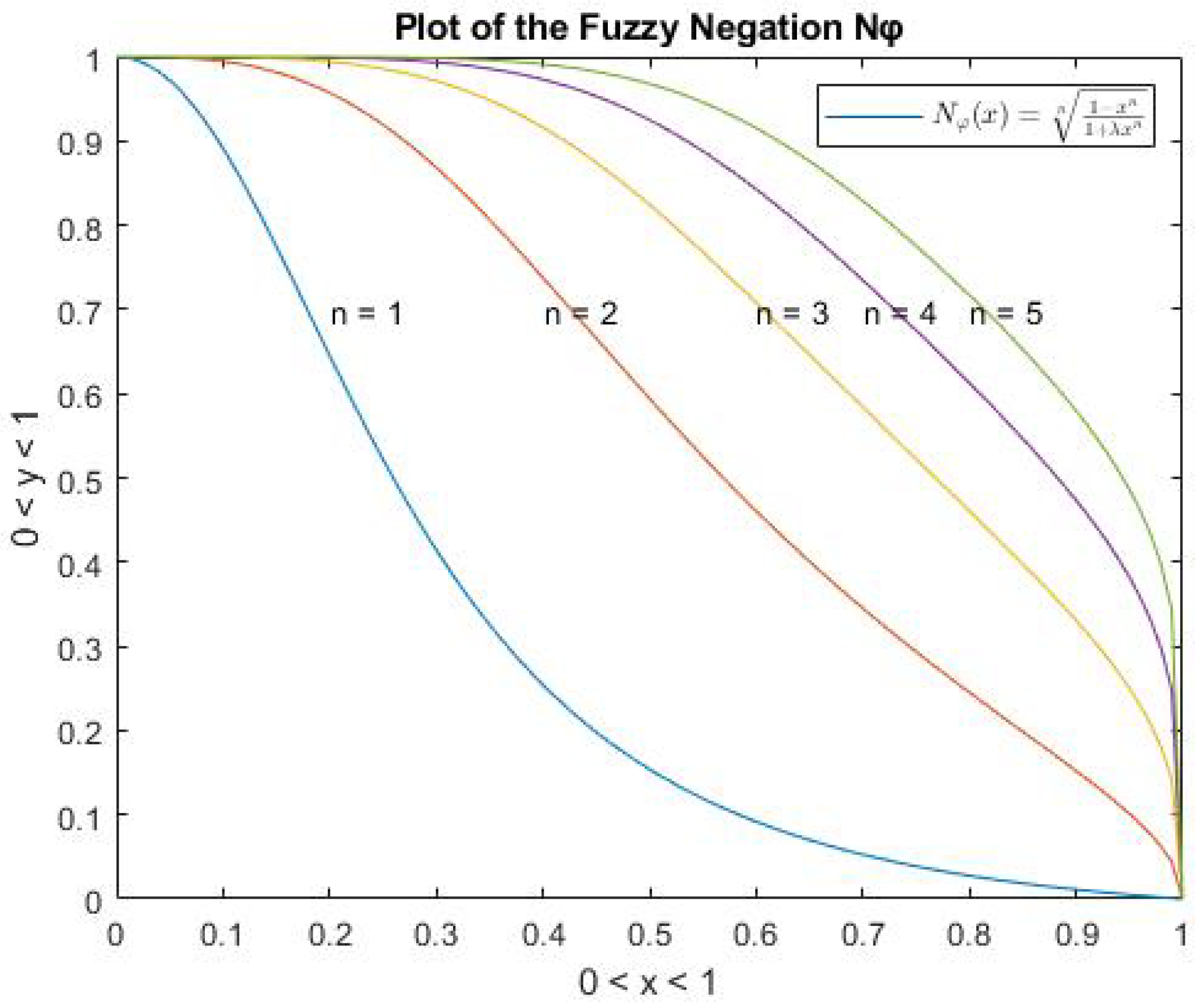
(i). Let N be a strong fuzzy negation of the Sugeno class: $N\left(x\right)=\frac{1-x}{1+\lambda x},\lambda \in (-1,+\infty )$

From Formula (1) of Theorem 1:

$$N_{\phi }\left(x\right)=\sqrt[n]{\frac{1-x^n}{1+\lambda x^n}},\lambda \in (-1,+\infty ),n\in N^{\ast }.$$

(7)

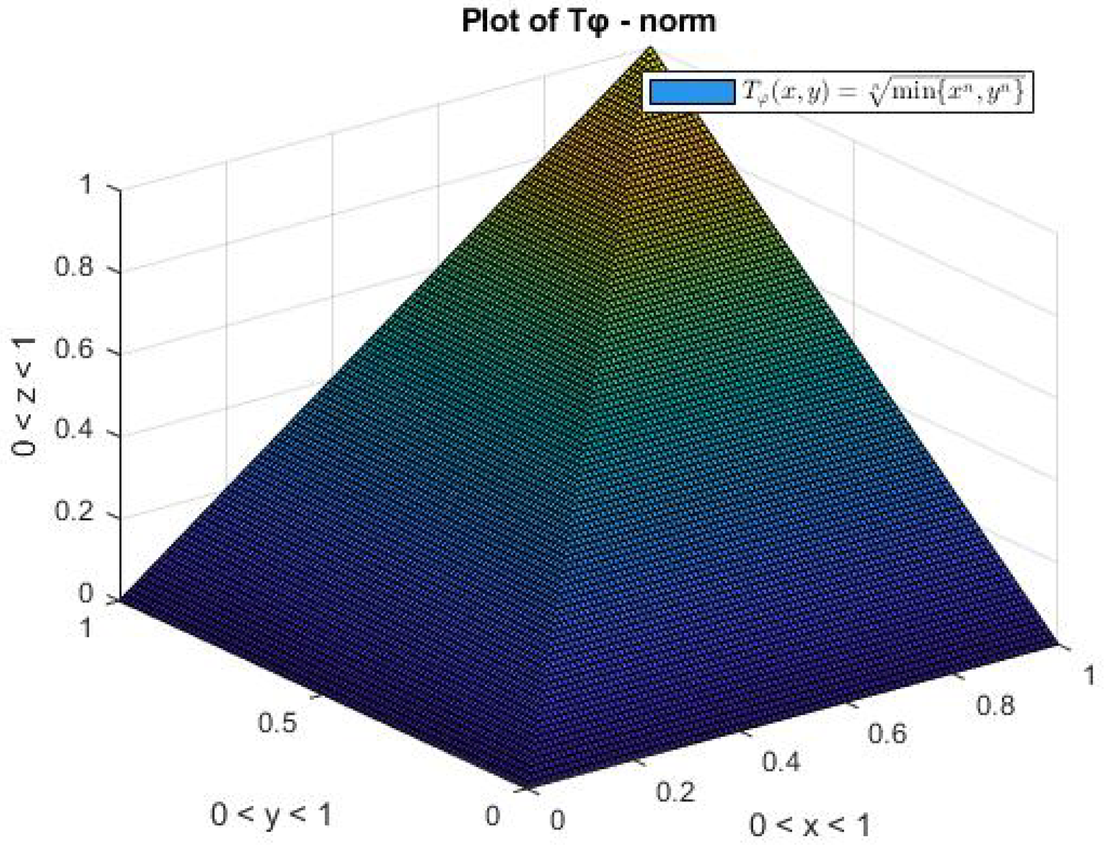
(ii). Let $T_M$ be a strict t-norm $T_M(x,y)=min\{x,y\}$.

From Formula (2) of Theorem 2:

$$T_{\phi }(x,y)=\sqrt[n]{min\{x^n,y^n\}},\forall x,y\in [0,1],n\in N^{\ast }.$$

(8)

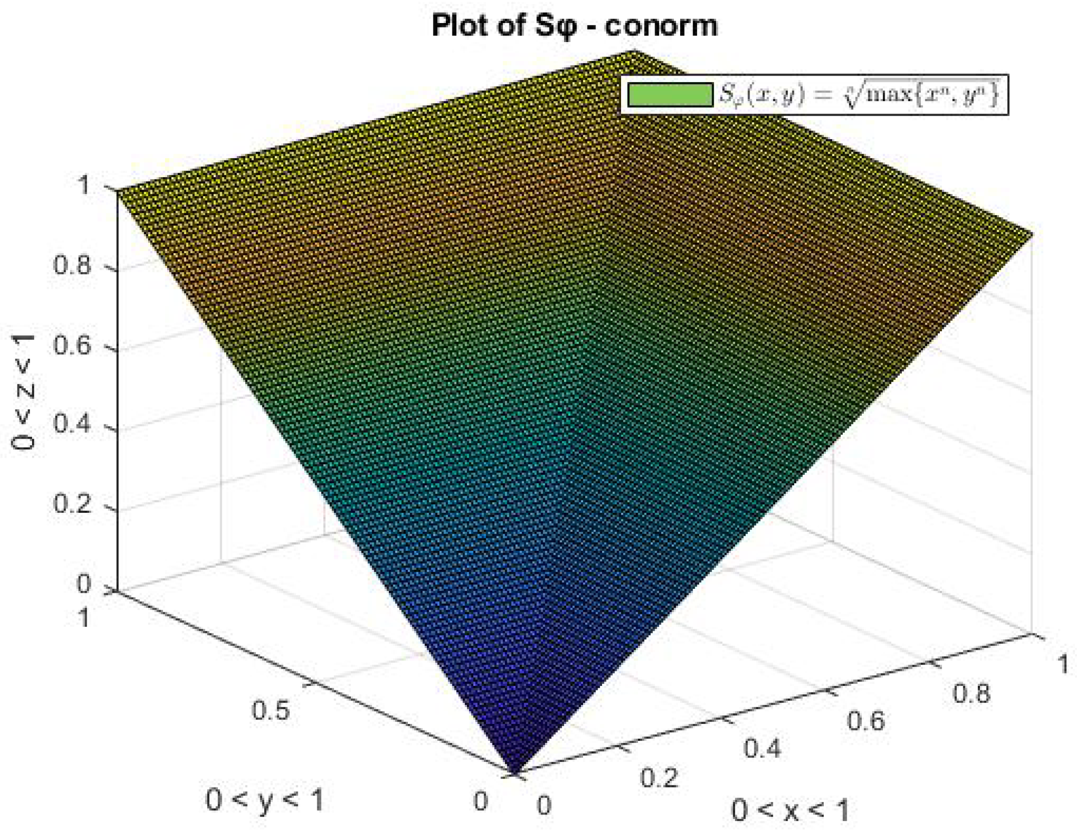
(iii). Let $S_M$ be a strict t-conorm $S_M(x,y)=max\{x,y\}$.

From Formula (3) of Theorem 3:

$$S_{\phi }(x,y)=\sqrt[n]{max\{x^n,y^n\}},\forall x,y\in [0,1],n\in N^{\ast }.$$

(9)

(iv). Alternatively, the S-conorm can be defined from Formula (4) of Theorem 4:

$$S_{\phi }(x,y)=1-\sqrt[n]{min\{{(1-x)}^n,{(1-y)}^n\}},\forall x,y\in [0,1],n\in N^{\ast }.$$

(10)

(v). In addition, the S-conorm can be defined from Formula (5) of Theorem 5:

$$S_{\phi }(x,y)=\sqrt[n]{\frac{1-min\{\frac{1-x^n}{1+\lambda x^n},\frac{1-y^n}{1+\lambda y^n}\}}{1+\lambda min\{\frac{1-x^n}{1+\lambda x^n},\frac{1-y^n}{1+\lambda y^n}\}}},\forall x,y\in [0,1],\lambda \in (-1,+\infty ),n\in N^{\ast }.$$

(11)

(vi). Let N be a strong fuzzy negation of the Sugeno class $N\left(x\right)=\frac{1-x}{1+\lambda x},\lambda \in (-1,+\infty )$, and $T_M$ be a strict t-norm $T_M(x,y)=min\{x,y\}$.

From Formula (6) of Theorem 6:

$$I_{\phi }(x,y)=\sqrt[n]{\frac{1-min\{x^n,\frac{1-y^n}{1+\lambda y^n}\}}{1+\lambda min\{x^n,\frac{1-y^n}{1+\lambda y^n}\}}},\forall x,y\in [0,1],\lambda \in (-1,+\infty ),n\in N^{\ast }.$$

(12)

(i). It is easy to see that a function defined by (7) is an involution with the following properties: $N_{\phi }\left(0\right)=1$ and $N_{\phi }\left(1\right)=0$. It is also strictly decreasing. Hence, $N_{\phi }$ is a strong negation function.

The Figure 2 is shown below.

(ii). It is easy to see that a function defined by (8) is a strict and Archimedean t-norm. The function $T_{\phi }$ is commutative and associative and it satisfies the boundary condition.

The Figure 3 is shown below.

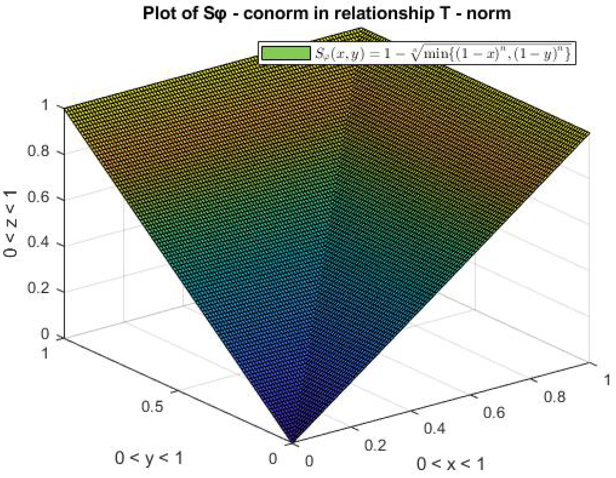
(iii). It is easy to see that a function defined by (9) is a strict and Archimedean t-conorm. The function is commutative, associative and monotonous and it satisfies the boundary condition.

The graph is shown below.

(iv). It is easy to see that a function defined by (10) is a strict and Archimedean t-conorm. The function $S_{\phi }$ is commutative, associative and monotonous and it satisfies the boundary condition.

The graph is shown below.

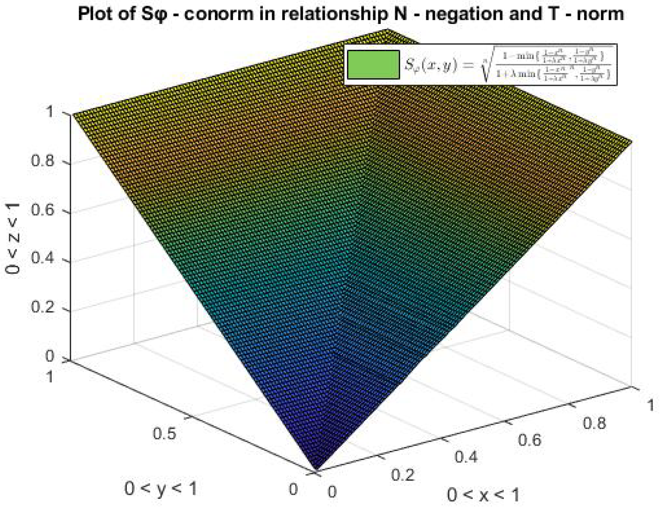
(v). It is easy to see that a function defined by (11) is a strict and Archimedean t-conorm.

The function $S_{\phi }$ is commutative, associative and monotonous and it satisfies the boundary condition.

The graph is shown below.

Remark 1.

Figure 4, Figure 5 and Figure 6 are observed to have the same graph. Therefore, we conclude that the S t-conorms given by Theorems 3–5 express the same S t-conorm.

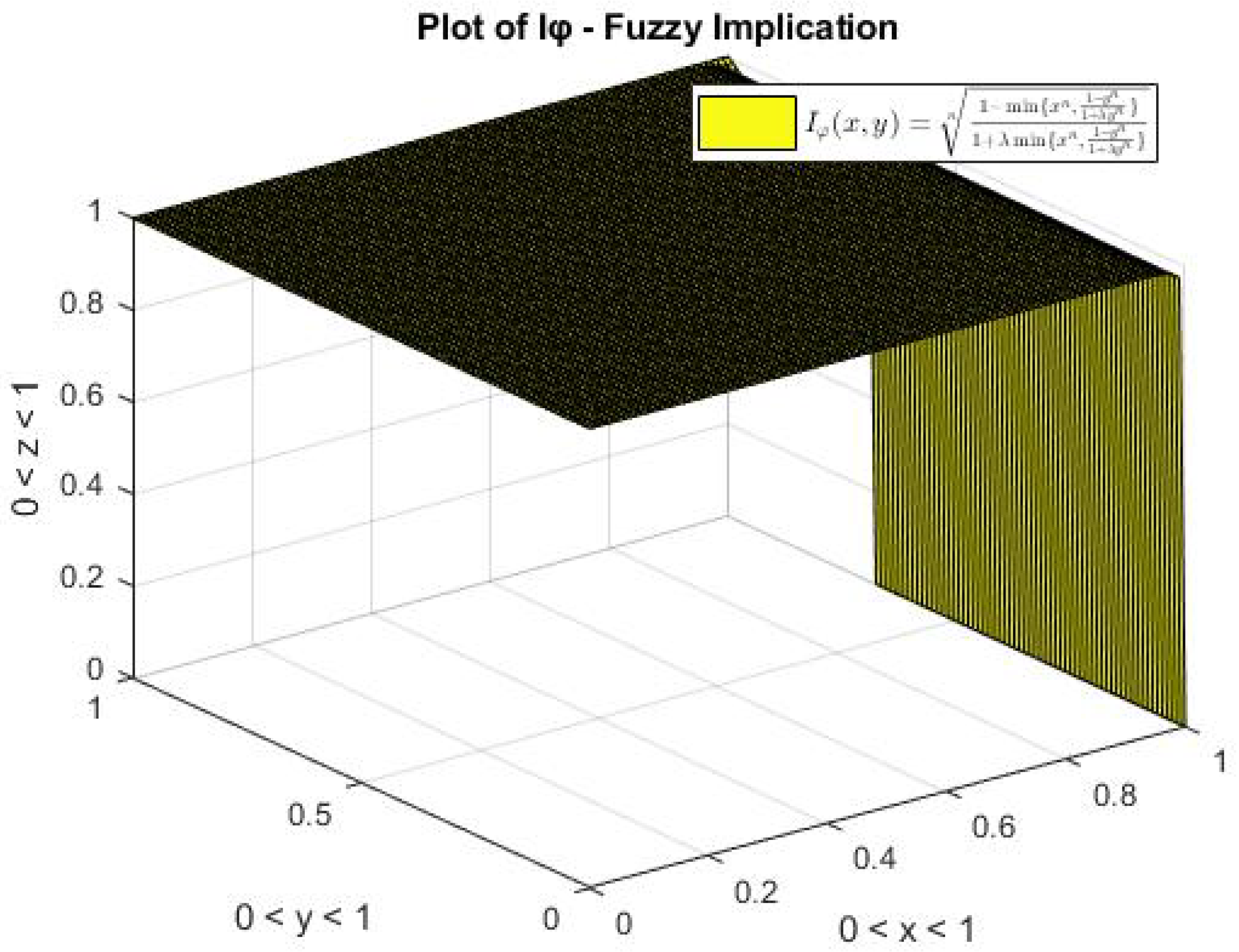
(vi). The function $I_{\phi }$ satisfies the properties of the family of fuzzy implications.

The Figure 7 is shown below.

5. Results

The result of this paper is an improved method of generalizing fuzzy connectives. The way this strategy improves on previous strategies is by being capable of generalizing any fuzzy connective instead of a select few. The conclusion drawn from the creation of this new method is that any fuzzy connective can be generalized (see Equations (1)–(6)).

The motivation behind this paper is the fact that the field of the generalization of fuzzy connectives has been inactive since 2012. Furthermore, the development of the approximate reasoning field, by producing new fuzzy connectives, was another motivation behind our research.

6. Discussion

The field of research of fuzzy connectives has been explored by multiple researchers over the years. As a result, multiple strategies for generalizing fuzzy connectives have been discovered. This paper focused on their limitations and provided solutions, which resulted in the creation of a new strategy. The various applications of this new method, as well a their results, are visible in the following paragraphs.

To be more specific, fuzzy connectives using the natural negation have been generated in the past (see J.C. Fodor and M. Roubens, Theorem 1.1, p. 4, [14]), (Gottwald S., Theorem 5.2.1 p. 86, [6]) and (Fodor J., p. 2077, [19]). However, the limitation is that this strategy involves only the natural negation in the process of generalizing the fuzzy connectives. The strategy presented in this paper, though, is capable of replacing the natural negation with any strong negation. This allows for the creation of new fuzzy connectives capable of involving all negations in the process of generalization.

Furthermore, fuzzy connectives using the T-Minimum, T-Product and T-Lukasiewicz t-norms have been generated in the past (see René B. et al., Theorem 2.3, p. 372, [20]). In addition, Gottwald S., Theorem 5.1.3, p. 82, [6] worked with such functions, but they focused mainly on the specific forms of t-norms (see

Table 4. Basic t-norms.

Designation	Equation
Minimum	$T_M(x,y)=min\{x,y\}$
Algebraic product	$T_p(x,y)=x·y$
Lukasiewicz	$T_{LK}(x,y)=max(x+y-1,0)$

). However, the limitation is that this strategy involves only these specific t-norms in the process of generalizing the fuzzy connectives. The strategy presented in this paper, though, is capable of replacing the T-Minimum, T-Product and T-Lukasiewicz t-norms with any t-norm. This allows for the creation of new fuzzy connectives capable of involving all t-norms in the process of generalization.

Moreover, this paper presents the generalization of fuzzy connectives using S-conorms. The prospect of incorporating S-conorms in the process of generalizing fuzzy connectives has not been explored in the past. In order to achieve this, the new strategy is based on the strategies mentioned before.

In addition, a strategy employing S-conorms, t-norms as well N-negations in the process of generalizing fuzzy connectives is explored in this paper. Such a strategy has not been implemented by someone else before.

Finally, a strategy for generalizing the classes of the I-implications was discovered in the past (see Bustince H., Burillo P. and Soria F. in 2003 ( [17]). Callejas C., Marcos J. and Bedregal B., in 2012, created the fifth strategy (see Figure 8), which generates any fuzzy implication ([18]). In this paper, however, a new method of generalizing I- implications with a combination of N-negations and t-norms is presented. This method will play a crucial role in future research, as it allows for the generalization of I-implications, which, in conjunction with weather data, can provide a better understanding of climate change.

7. Conclusions

The objective of this paper was to create a new strategy for generalizing fuzzy connectives which is more flexible and faster in comparison with the rest. The way this objective was achieved was by solving the limitations of previous methods. To be more specific, with this new strategy, a wider range of fuzzy connectives and automorphisms is utilized in the process of generalization.

References

- Menger, K. A survey on fuzzy implication functions. Proc. Natl. Acad. Sci. USA 1942, 28, 535–537. [Google Scholar] [CrossRef] [PubMed] [Green Version]
- Schweizer, B.; Sklar, A. Probabilistic Metric Spaces; Dover Publications, Inc.: Mineola, NY, USA, 1983. [Google Scholar]
- Ling, C.H. Representation of associative functions. Publ. Math. Debr. 1965, 12, 189–212. [Google Scholar]
- Frank, M.J. On the simultaneous associativity of f(x,y), and x+y-f(x,y). Aequ. Math. 1979, 19, 194–226. [Google Scholar] [CrossRef]
- Mirko, N. Characterization of Measures Based on Strict Triangular Norms. J. Math. Anal. Appl. 1999, 236, 370–383. [Google Scholar]
- Gottwald, S. A Treatise on Many-Valued Logics; Research Studies Press: Baldock, UK, 2001; pp. 63–105. [Google Scholar]
- Klement, E.P.; Mesiar, R.; Pap, E. Triangular Norms; Kluwer: Dordrecht, The Netherlands, 2000; pp. 4–10, 108–110. [Google Scholar]
- Kerre, E.E.; Huang, C.; Ruan, D. Fuzzy Set Theory and Approximate Reasoning; Wu Han University Press: Wuhan, China, 2004. [Google Scholar]
- Trillas, E.; Mas, M.; Monserrat, M.; Torrens, J. On the representation of fuzzy rules. Int. J. Approx. Reason. 2008, 48, 583–597. [Google Scholar] [CrossRef] [Green Version]
- Kerre, E.; Nachtegael, M. Fuzzy techniques in image processing. In Studies in Fuzziness and Soft Computing; Springer: New York, NY, USA, 2000; Volume 52. [Google Scholar]
- Bustince, H.; Mohedano, V.; Barrenechea, E.; Pagola, M. Definition and construction of fuzzy DI-subsethood measures. Inf. Sci. 2006, 176, 3190–3231. [Google Scholar] [CrossRef]
- Baczyński, M.; Jayaram, B. On the characterization of (S,N)-implications. Fuzzy Sets Syst. 2007, 158, 1713–1727. [Google Scholar] [CrossRef]
- Mas, M.; Monserrat, M.; Torrens, J.; Trillas, E. A survey on fuzzy implication functions. Proc. IEEE Trans. Fuzzy Syst. 2007, 15, 1107–1121. [Google Scholar] [CrossRef]
- Fodor, J.C.; Roubens, M. Fuzzy Preference Modelling and Multicriteria Decision Support. In Theory and Decision Library, Serie D: System Theory, Knowledge Engineering and Problem Solving; Kluwer Academic Publishers: Dordrecht, The Netherlands, 1994; Volume D, pp. 3–16. [Google Scholar]
- Mas, M.; Monserrat, M.; Torrens, J. QL versus D-implications. Kybernetika 2006, 42, 351–366. [Google Scholar]
- Yager, R.R. On some new classes of implication operators and their role in approximate reasoning. Inf. Sci. 2004, 167, 193–216. [Google Scholar] [CrossRef]
- Bustince, H.; Burillo, P.; Soria, F. Automorphisms, negations and implication operators. Fuzzy Sets Syst. 2003, 134, 209–229. [Google Scholar] [CrossRef]
- Callejas, C.; Marcos, J.; Bedregal, B. Actions of Automorphisms on Some Classes of Fuzzy Bi-implications. SBMAC 2012, 177, 140–146. [Google Scholar]
- Fodor, J.C. Nilpotent Minimum and Related Connectives for Fuzzy Logics. In Proceedings of the 1995 IEEE International Conference on Fuzzy Systems, Yokohama, Japan, 20–24 March 1995; Volume 4, pp. 2077–2082. [Google Scholar]
- Benjamín, R.; Callejas, B.; Adriana, T. The best interval representations of t-norms and automorphisms. Fuzzy Sets Syst. 2006, 157, 3220–3230. [Google Scholar]
- Alsina, C. As You Like Them: Connectives in Fuzzy Logic. In Proceedings of the 26th International Symposium on Multiple-Valued Logic, Jantiago de Compostela, Spain, 19–31 January 1996; pp. 2–7. [Google Scholar]
- Baczyński, M.; Jayaram, B. Fuzzy Implications. In Studies in Fuzziness and Soft Computing; Springer: Berlin/Heidelberg, Germany, 2008; Volume 231. [Google Scholar]
- Bedregal, B.C. On Fuzzy Negations and Automorphisms. Ana. CNMAC 1984, 2, 1127–1129. [Google Scholar]
- Weber, S. A General Concept of Fuzzy Connectives, Negations and Implications Based on t-norms and T-Conorms On the representation of fuzzy rules. Fuzzy Sets Syst. 1983, 11, 115–134. [Google Scholar] [CrossRef]
- Trillas, E. Sobre funciones de negacin en la teora de conjuntos difusos. Stochastica 1979, III, 47–60. (In Spanish) [Google Scholar]
- Shi, Y. A Deep Study of Fuzzy Implications. Ph.D. Thesis, Ghent University, Ghent, Belgium, 2009; pp. 5–22. [Google Scholar]
- Fodor, J. On fuzzy implication operators. Fuzzy Sets Syst. 1991, 42, 93–300. [Google Scholar] [CrossRef]
Figure 1.
The history and evolution of t-norms.
Figure 2.
Fuzzy negations generated from Sugeno class using an automorphism function.
Figure 3.
t-norm generated from using an automorphism function.
Figure 4.
S-conorm generated from using an automorphism function.
Figure 5.
Figure 6.
Figure 7.
I-implication generated from using an automorphism function.
Figure 8.
The history and evolution of fuzzy implications.