Article

Assessing Environmental Justice at the Urban Scale: The Contribution of Lichen Biomonitoring for Overcoming the Dichotomy between Proximity-Based and Distribution-Based Approaches

Department of Life Sciences, University of Siena, Via P.A. Mattioli 4, 53100 Siena, Italy
*
Author to whom correspondence should be addressed.
Atmosphere 2024, 15(3), 275; https://doi.org/10.3390/atmos15030275
Submission received: 15 January 2024 / Revised: 20 February 2024 / Accepted: 23 February 2024 / Published: 25 February 2024

Abstract

:
In this study, we tested the use of lichen biomonitoring techniques for the assessment of air quality disparities at the urban scale. We based our evaluation on the results of a previous lichen biomonitoring study carried out in Milan (Northern Italy), which estimates the contamination by potentially toxic elements (PTEs) and its distribution over the area, also providing an evaluation of the main emission sources. Therefore, we used the traditional methodologies for environmental justice assessment: the proximity-based and the distribution-based approaches. The workflow we propose is a data-driven selection of emission sources that contributes to overcoming the dichotomy between the two approaches and is now widely debated in the scientific community. A socio-economic deprivation index was elaborated for each census unit of Milan city and then related to the proximity of the emission sources previously selected. The results suggested that in the surrounding of industries and railways, the deprivation is higher, while the proximity of main roads is inhabited by wealthier populations. The distribution-based approach was run through a quantile regression analysis, and the outcome indicated that among the wealthier groups, an increase in contamination is followed by an increase in socio-economic deprivation, whilst among the deprived groups, people with greater economic opportunities tend, however, to live in worse air quality conditions due to the proximity of communication routes. This study poses the potential to review the classical methods of EJ assessment, providing a reliable workflow applicable in urban areas—the most vulnerable in terms of air quality disparities in the present and in the future.

1. Introduction

During recent decades, the relationship between air quality and human life quality has been deeply investigated. Prolonged exposure to polluted air could lead to physical and mental health problems such as asthma, cardiovascular diseases, and even depression and reduced well-being, among many others [1,2]. On the other side, good air quality positively affects several aspects of life, such as personal satisfaction and work productivity [3,4]. However, as a matter of fact, it has become clearly evident worldwide that the costs and benefits of air quality are not evenly distributed among the population, both locally and globally. The first studies about “Environmental Justice” (EJ), i.e., the study of the environmental disparities between population groups, were carried out in the late 1970s in the USA by [5], who showed that the territories with a larger proportion of Afro-American people were more likely to be targeted for dangerous power plants and industries than those with a white majority. Even though in the USA a sort of “Environmental Racism” is still ongoing [6,7], many recent studies carried out in Europe and other Western cities are consistent in stating that, so far, socio-economic status is the main driver for environmental quality disparities [8]. Indeed, ref. [9] evaluated the personal exposure to air pollution in London, concluding that the residential exposure to NO2 was significantly higher in people with a lower income (<GBP 10,000), and similar findings were presented for the metropolitan region of Barcelona by [10], Dunkerque agglomeration (Northeastern France) by [11], and Mexico City by [12]. The disadvantaged groups, therefore, live the so-called “triple jeopardy”, i.e., the combination of low economic power, low environmental quality, and the heavier consequences of both these factors on life and health quality, if compared with wealthier groups [13]. Thus, it is of primary importance to assess these disparities in order to plan specific territorial policies for local and global sustainable development. At an urban scale, this topic is particularly urgent since the urban population is constantly growing, and a well-planned territory might reduce extreme differences, enabling everyone to live in a clean environment and to have a better quality of life [14]. Given the novelty of this discipline, a methodological consensus for its study has not been reached yet; however, two main approaches are now being used to assess the disparities in air pollution exposure between population groups: proximity-based and distribution-based. The “proximity-based” approach relates the socio-economic status of people to the proximity of pollutants plants and/or heavy industrialized areas. This method implicitly takes into account the social organization in urban sites, highlighting aspects as segregation or neighborhood quality, but it fails to enlighten the real exposure of population to air pollution [15]. The “distribution-based” approach, on the contrary, takes into account the real air quality distribution, regardless of the presence or distance to industrial plants. Thus, in this case, the approach better meets the necessity to evaluate the personal exposure to air pollution, with less attention paid to aspects such as segregation and urban organization [15]. However, some considerations should be noted. The proximity-based approach is undergoing an intense debate since it is related to a primary view of EJ that was firstly advanced by [5]. In fact, by considering just the presence but not the real impact of the single emission sources on air quality, there is the risk of simplifying the evaluation of Environmental Justice too much, shifting more to a “urban justice” concept [16,17,18]. For the distribution-based approach, instead, the issue lies in the dealing of air quality data. Many authors, in fact, obtain data on air pollution directly from local repositories or already modeled data, which derive from the traditional monitoring devices deployed in the study area [19,20,21]. These devices are often present in small numbers due to their high costs of installation and maintenance, providing coarse-grained maps of air pollution that fail to catch the small variations inside the city. When matching these coarse data with the very fine-grained data of socio-economic deprivation (which, contrastingly, are elaborated according to census traits or zip codes), a low accuracy of Environmental Justice assessment is often possible. This lack of resolution of air pollution maps is emerging as a very prohibitive and determinant issue to cope with EJ assessment, and many authors report this as one of the main problems in this kind of study [21,22,23]. Moreover, the traditional devices are very accurate in measuring the concentration of specific contaminants, but they cannot provide information on the interaction of compounds and their effect on the biota.
In this work, we propose the use of lichen biomonitoring techniques to contribute to overcoming these flaws. Lichens are symbiotic organisms formed by a mycobiont, generally an ascomycete, and a photobiont, usually green algae. Contrarily to higher plants, lichens lack stomata, waxy cuticles, and roots, and the nutrients are absorbed through the entire surface of their thallus (body) from wet and dry atmospheric depositions. Lacking protective structures, lichens are particularly sensitive to changes in air elemental composition, reflecting rapidly and clearly even air pollution episodes. In addition, many species are great bio-accumulators of potentially toxic elements (PTEs), showing both the presence and the bio-availability of these airborne contaminants [24,25,26]. The cost-effectiveness of the analysis combined with the considerable availability of lichen material make it possible to transplant lichens into the study area according to the aim of the research, improving the sampling effort where it is required and obtaining a fine-grained map of the biological impact of air pollution over the study area. Lichens have been successfully used to biomonitor biological impacts of air pollution in urban [27], rural [28], and industrial [29] areas and even indoors [30]. Notwithstanding the great potential of this approach, lichen biomonitoring techniques are underexploited for EJ assessment, with just a few scientific contributions: A first study was carried out in Dunkerque agglomeration, an industrial and densely populated area (Northern France), by [11], using lichens as bioaccumulators of PTEs. The authors collected samples of native lichens from tree trunks in 60 sampling stations and then compared the bioaccumulation values with the socio-economic status of the population at a very fine level. A second study was carried out by [31] in an area with a municipal solid waste incinerator in Northern Italy. In that case, the authors used lichen transplants following a specific sampling design in order to maximize the sampling effort around the incineration plant. Their findings showed both the biological impact of air pollution and the air quality disparities occurring in the area. Both studies ([11,31]) showed how the lichen biomonitoring provided detailed spatial data of air pollution that were translated into a reliable map of air quality disparities. However, in both cases, the authors only used the “distribution-based” approach, while the main emission sources of air pollution were just hypothesized (industries and the incinerator plant). In our opinion, a novel and more complete approach is possible by including the “distribution-based” and the “proximity-based” approaches in the same study of EJ assessment.
The aim of this study is to propose an approach in which the versatility of lichen biomonitoring techniques is used to overcome the methodological issues in EJ assessment, starting from already published data of lichen biomonitoring campaign. In particular, we test: (i) the “distribution-based” approach by matching the distribution of air contamination measured through lichens with the socio-economic characteristics of the population; and (ii) the “proximity-based” approach by considering the socio-economic characteristics of the population that lives in the surrounding area of the main emission sources of air pollution, detected through lichen biomonitoring.

2. Materials and Methods

2.1. Dataset

For this study, we have used already published data of a lichen biomonitoring study carried out in Milan, Northern Italy, using the lichen species Evernia prunastri (L.) Ach. as a bioaccumulator of PTEs [32]. The details of the lichen biomonitoring procedure are reported in [32]. In brief, lichen samples were collected in an unpolluted area of Tuscany (Central Italy, coordinates: 43°07′31.47″ N, 11°21′43.85″ E) in December 2018 and exposed for 3 months at 50 sampling sites (three lichen bags for each station) in the city of Milan.
After the exposure, the content of Al, As, Cd, Cr, Cu, Fe, Pb, Sb, and Zn was measured by ICP-MS. The samples showed a significant bioaccumulation of Cr, Cu, Fe, Sb, and Pb. The element concentrations served to elaborate the Pollution Factors and the Contamination Index. The Pollution Factors highlighted the spatial patterns of specific contaminations (details below), while the Contamination Index (CI) was calculated as the geometric mean of the bioaccumulated elements according to (1) (an extensive description is reported in [31]) to describe the overall contamination of the study area.
C I i = E C e l 1 × E C e l 2 × E C e l n   n
where CIi is the Contamination Index in the ith site; EC = Exposed-to-Control ratio; that is, the concentration (ppm) in the exposed sample on the concentration (ppm) of the control sample. Those elements with a median EC > 1 in the whole area and an EF > 10 (EF = Enrichment Factor—an index that considers the soil contribution to the final concentration found in lichen samples, see [31]) were considered for the elaboration of the EC in each sampling site.
A scheme of the workflow is reported in Figure 1.
This study [32] has been selected for the following reasons:
-
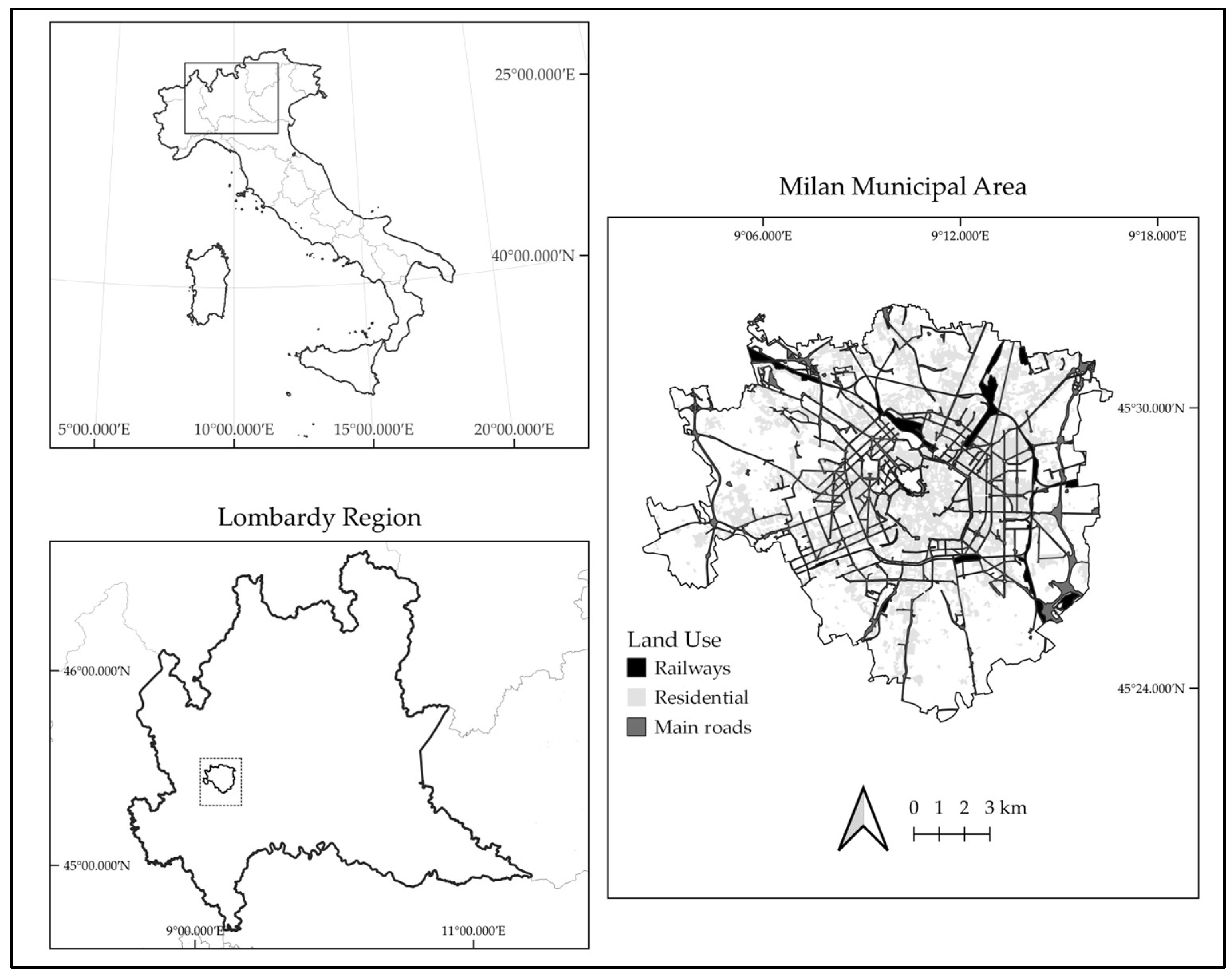
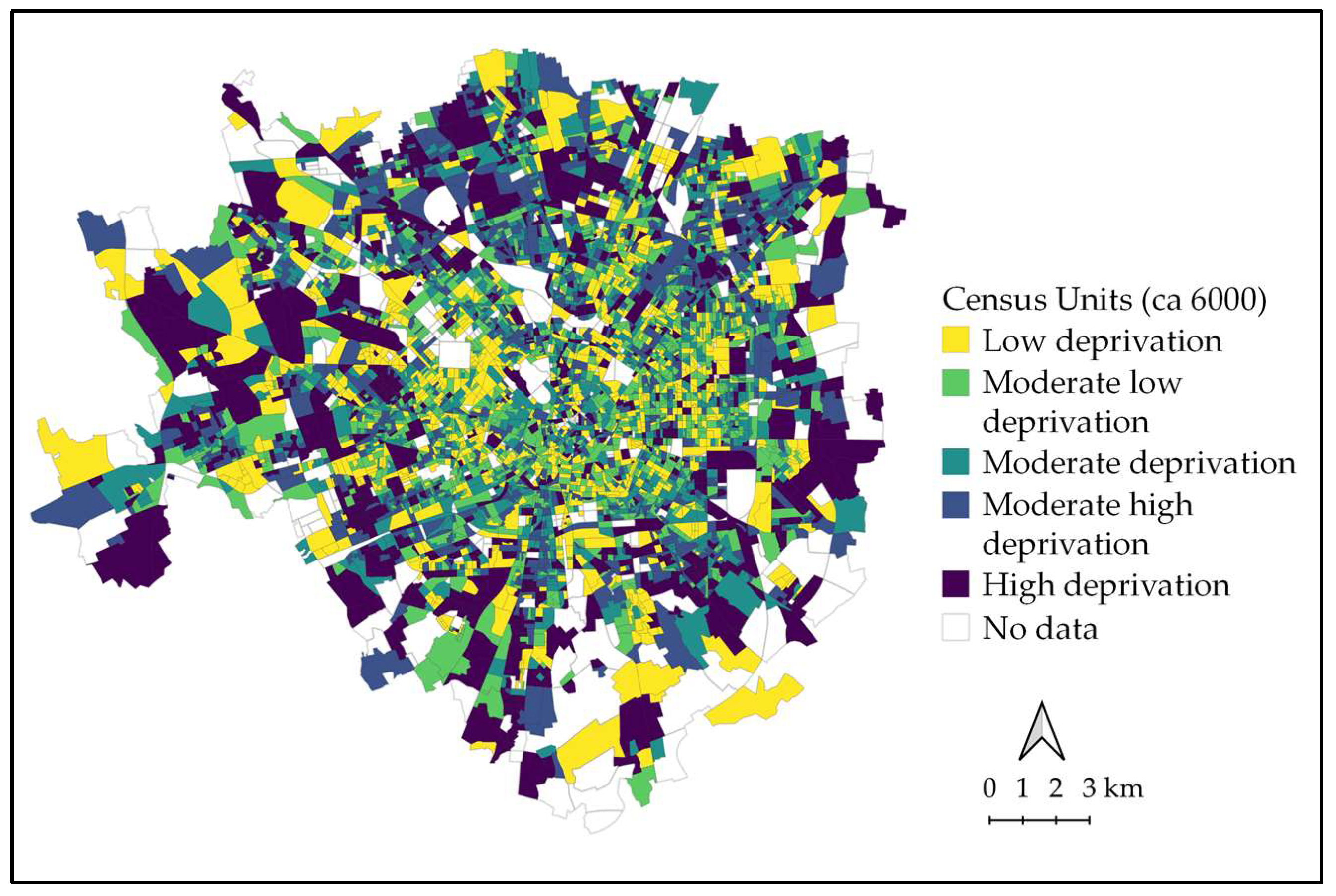
The sampling effort was homogeneous all across the city, with a high number of sampling sites (50 sites over 181 km2) (Figure 2). Therefore, a reliable representation of the city as a whole is provided, and the match with socio-economic variables is not spatially biased by the clustering of the observations. Moreover, the high number of sampling sites allows for a fine-grained map of the results over the area.
-
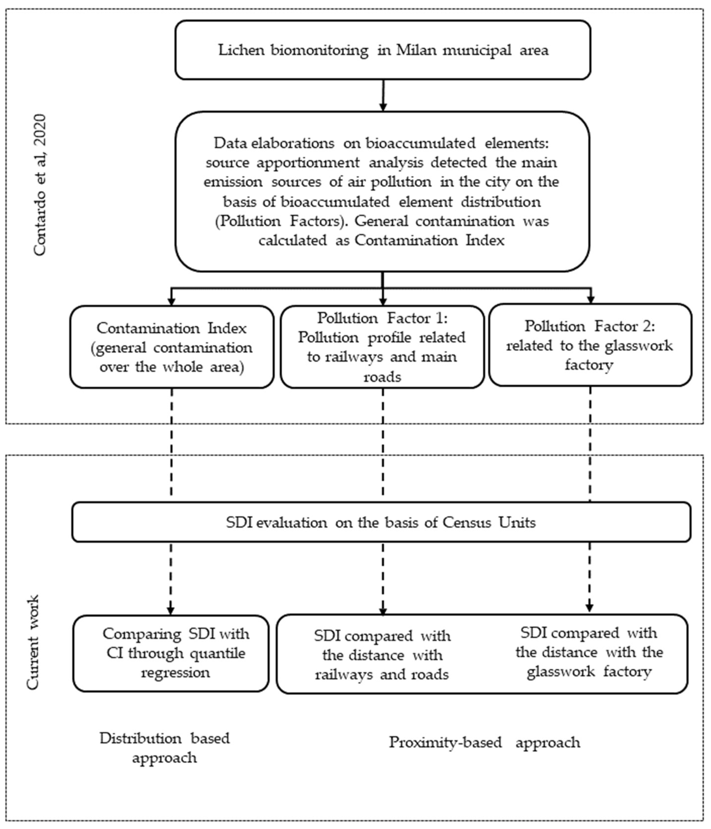
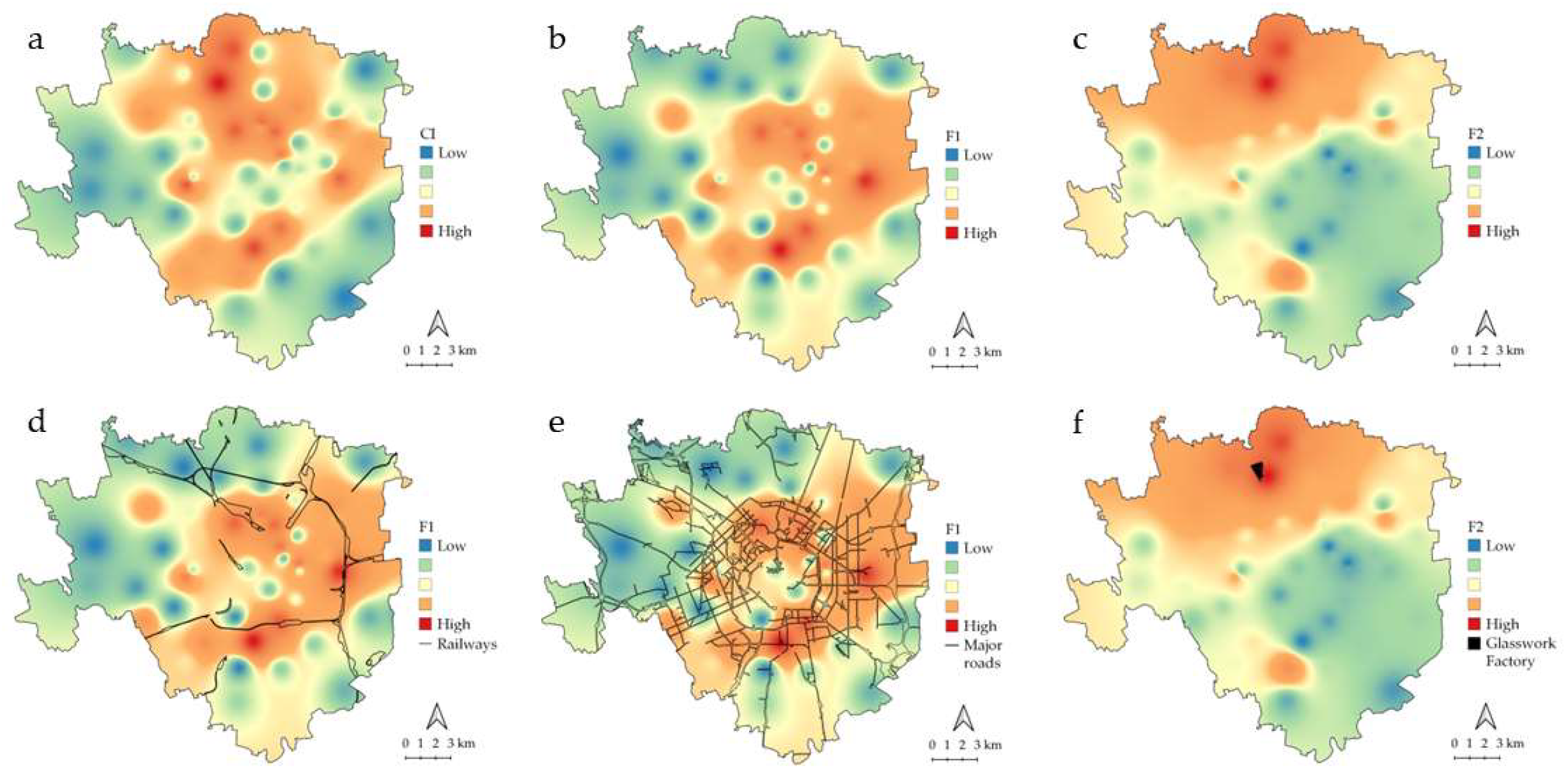
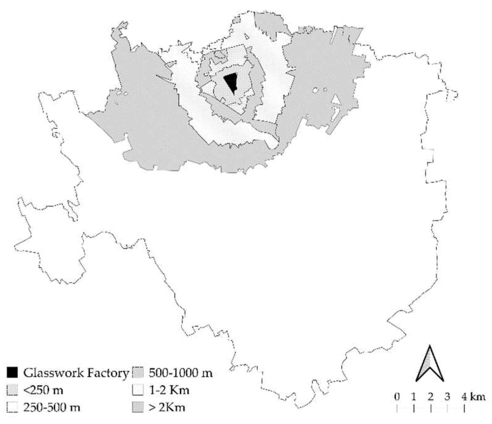
It outlined the main sources of airborne PTEs in Milan and provided spatial patterns of pollution. Namely, a first pollution factor (F1) identified non-exhaust emissions from vehicular traffic and railway lines (Figure 3b), while a second pollution factor (F2) identified the activity of an industrial area located in the northern part of the city, especially a former glasswork factory, as the main emission source (Figure 3c). The details about the statistical method and the individuation of the emission sources are reported in [32].
-
It provided a “general contamination” (Contamination Index, CI) distribution over the city of Milan, elaborated on the basis of all the bioaccumulated elements taken as a whole. These data are used here to apply the distribution-based approach (Figure 3c).
-
Milan urban area is a typical European city; thus, it could be representative of the dynamics occurring in Europe as well as in other large Western cities (see further).

2.2. Study Area

Milan is among the most important Italian cities for its central role in the economy of the country. It hosts 1.4 million inhabitants and 1 million city users every day in an area of 181 km2. This city represents a model case study for the assessment of EJ in urban areas because, in the past century, it went through radical changes in its economy, shifting from an industry-based to a service-based economy. The great transformations modified the urbanistic assets as well as the social organization, with a decrease in primary industry workers and an increase in tertiary industry ones, thus carrying new needs and requirements for the life of citizens. These processes are still ongoing, and the city is facing a fast modernization, periphery renewal, and an increase in green areas [33]. Indeed, Milan is among the most polluted cities in Europe by PM2.5 due to the dense industrial and residential land use in which it is embedded, underpinned by a humid–continental climate that favors air stagnation and thermal inversions, literally keeping air pollution over the area for long periods. The air pollution problem has been addressed by local administrations in many ways, e.g., blocking vehicular traffic on certain days, increasing pedestrian and low-traffic areas, and preventing the most-polluting vehicles from entering the city center. These great changes caused an increase in house prices and the cost of living, pressing the people’s movement into the city, according to their needs and economic possibilities. Based on these features, it is reasonable to hypothesize that wealthier groups tend to live in better areas for air quality and the presence of services, which are more expensive, while the disadvantaged groups occupy lower-quality areas both for services and air quality.

2.3. Evaluating the Socio-Economic Status in the Milan Urban Area

To assess if socio-economic status is a determinant factor for the air quality experienced, we elaborated a socio-economic deprivation index at the smallest spatial scale available for the city, i.e., the census unit scale. Census units in Milan are ~6000 and are not homogeneous in size and number of inhabitants, but they are the basis for regional management. Demographic data were taken from the Italian National Institute of Statistics (ISTAT), and they were available for the census campaign of 2011 [34]. The socio-economic deprivation index (SDI) was elaborated following the method proposed by [35] considering the following factors: unemployment rate, school degree, population density, number of family members, and house renting (Table 1). The index is calculated as the sum of all the ratios within each census unit. For example, the “Low Schooling” parameter was calculated as follows:
(n of illiterate + n of literate + n of people with primary and secondary school)/total of the population of the given census unit.
Accordingly, all the other ratios were calculated and then summed together.
We excluded from the elaborations all the census units with no inhabitants and those with missing parameters, obtaining a final number of ~5500 census units.

2.4. Environmental Justice

On the basis of the lichen biomonitoring results described in [32], we were able to test both the main approaches for EJ assessment, i.e., the proximity-based and the distribution-based approaches.

2.4.1. Proximity-Based Approach

The proximity-based approach was used taking into account the distance (m) from the main pollution sources that emerged from the lichen biomonitoring study: railway lines, main roads, and industry.
The distance to major roads and railways was calculated from the centroid of each census unit to the closest railway line and major roads, separately. Then, the distances were sorted into deciles and the median of each decile was correlated as a response variable with the median of the respective deciles of socio-economic status using the Spearman correlation coefficient.
For the industry, a different approach was used. Since the contamination was mostly concentrated in a specific area, was the most industrialized, and had a clear hotspot corresponding to a glasswork factory, we shaped four different distance classes starting from the glasswork factory, namely 0–250 m, 250–500 m, 500–1000 m, and 1000–2000 m (Figure 4). For each class, the median SDI was calculated. Differences between SDI values within classes of distance were checked using Kruskal–Wallis, ANOVA, and the Conover–Iman test for pos-hoc comparisons.

2.4.2. Distribution-Based Approach

The overall contamination pattern in the study area, as emerged from the lichen biomonitoring survey, was used to run the distribution-based approach. To find a relationship between socio-economic status and air pollution exposure, we assigned to each census unit a value of contamination, calculated as the mean of the values of all the pixels of the contamination raster inside the polygons of census units using the Zonal Statistics geoprocessing tool of QGIS. In this way, for each unit, we obtained both the SDI and the CI. To describe the possible relationship between CI and SDI, we used the quantile regression method. Quantile regression has the advantage of estimating conditional quantile functions, thus providing a suitable method for describing the different responses across quantiles of the distribution of the response variable [36,37]. This method does not require any assumption about the normality of the residuals and is especially robust to extreme values and outliers, allowing us to describe the complex relationship between the variables. In EJ assessment, this method is experiencing an increasing interest [9,12]. We choose to take CI as the independent variable and SDI as the dependent one. This choice was driven by the fact that main pollution sources are, at the moment, quite stable, and we assume that people live and are distributed in the city according to their economic possibilities. Also, in this case, variables were sorted into deciles. An Ordinary Least Square (OLS) regression was run to check for differences between the methods. All statistical evaluations were run using the free R software (R Core Team, Vienna, Austria, 2022. Version 4.0.3), package quantreg [38].

3. Results

The socio-economic deprivation index was elaborated for each census unit and then sorted into quantiles; its distribution is reported in Figure 5.

3.1. Proximity-Based Approach

Features of the SDI within the Milan urban area are reported in Table 2. The mean SDI value for Milan city is 0.82, not considering that the industrial area SDI decreases at 0.81—a value that is significantly (p < 0.05) different from the SDI calculated for the industrial area only (0.87). Within this area, the distance classes showed significant differences in SDI values. The highest deprivations emerged at 500–1000 m (1.06) and 250–500 m from the glasswork factory. Then, after increasing the distance, the deprivation significantly decreases (0.91 for 1–2 km from the glasswork), until it reaches the mean value of Milan (0.82).
The results of the proximity-based approach are reported separately for the two main pollution profiles. The relationship of SDI with distance from major roads and railways as the result of a linear model is shown in Figure 6. A positive and robust (R2 = 0.8) relationship with distance from major roads emerged (Figure 6a), indicating that in the proximity of the main communication routes, the deprivation tends to be smaller, while disadvantaged groups live far (>500 m) from main roads. Opposingly, a still robust (R2 = 0.79) trend emerged for the distance from railway lines (Figure 6b), with higher SDI values in those census units surrounding (<500 m) these infrastructures and increasing the wellness of the population with increasing distances.

3.2. Distribution-Based Approach

The results of the quantile regression for the distribution-based approach (Table 3) show a significant influence of the contamination over the SDI in almost all quantiles. In particular, for the first four quantiles, a positive relationship emerged, while from the seventh onward, a negative relationship was evident between the variables. Thus, increasing the contamination in the less-deprived population, there is just a slight increase in deprivation, while in the most-deprived groups, as contamination increases, the deprivation tends to decrease.

4. Discussion

In this work, we tested the use of lichen biomonitoring techniques for Environmental Justice assessment at the urban scale. In particular, we applied the most common approaches used in EJ studies, i.e., proximity-based and distribution-based, on the basis of a lichen biomonitoring study of air pollution [32]. Indeed, the proximity analysis considers just the presence and distribution of pollution sources, assuming personal exposures are correlated to source proximity [39,40,41] while the distribution-based approach usually refers to coarse-grained data of air pollution from the few scattered monitoring equipment, that scarcely match the EJ assessment requirements [22]. Comparing the two methods, ref. [16] concluded that proximity analysis could be a good predictor of exposure only in some cases and only if flexibility is used, thus highlighting the great uncertainty related to this method. Despite some attempts to incorporate the two methods by including emission data to select the more impacting sources for the successive proximity analysis [42], the lack of fine-grained distribution maps hampers a real matching between methods; thus, more comprehensive methods are required in order to overcome these shortcomings [18].
The workflow suggested in this study is promising. Firstly, the lichen biomonitoring study [32] provided a high-resolution map of air pollution thanks to the high number of sampling sites scattered within the city. In fact, compared to other studies using physical-chemical monitoring devices, the lichen biomonitoring campaign described in [32] provided a density of 0.28 monitoring sites per km2 (50 sampling sites/181 km2), while [21] had just 0.014 monitoring sites per km2 in Hong Kong (15 monitoring sites/1106 km2). Moreover, ref. [22] had, among the investigated cities in their study in the Czech Republic, the highest number of monitoring devices in Praha with a density of 0.030 monitoring sites per km2 (15 monitoring sites in 496 km2), and ref. [23] had 0.006 monitoring devices per km2 in São Paulo (9 monitoring sites/1521 km2). Thus, our air quality biomonitoring network was ca. 20 times denser than in Hong Kong, 45 times denser than in São Paulo, and 9 times denser than in Praha. Secondly, the selection of the emission sources for the proximity analysis was data-driven from the distribution of pollutants, and their disentanglement in emission profiles provided useful information about the type of pollution. One pollution profile, in fact, was related to industry and linked to the industrial history of the city (the glasswork factory was dismissed in 2004), while the other profile was linked to modern pollution by vehicle non-exhaust emissions. Separating the pollution profiles allowed for a deeper and more specific assessment of exposure inequalities between population groups. Following a data-driven approach, this method is unbiased, not based on arbitrary knowledge of the territory, and successfully combines the two traditional methodologies.
Our findings from the proximity analysis around the glasswork factory showed significant differences in SDI values with distance. In particular, census units within the higher concentration area of the pollution profile related to industrial emissions, and the so-called “industrial area” showed a higher SDI than the rest of Milan (0.87 and 0.81, respectively), being in line with the theory of the disproportion of environmental hazards where disadvantaged groups live [43]. Considering the distance classes within the industrial area, an interesting trend was found: the closest census units showed no significant differences with the others, while SDI values increase significantly up to 1000 m [1.06], then decrease until they reach the Milan mean (0.82). These results further confirm the theory that disadvantaged groups experience a higher concentration of polluting sources [6,44]. However, the debate about “who came first: the pollution or the deprivation” is still open, and very rarely it is possible to have a reliable answer [45]. Still, to have a complete picture, one should study the evolution in time of both socio-economic deprivation and urban assets, and this is not always feasible due to the lack of data. It is reasonable to assume that, in our case, people living in this area are the former workers of the factory, who have remained there after industrial closure.
Performing the proximity analysis on the basis of main roads and railways, different and opposite results emerged. Even though both are sources of non-exhaust emissions, it seems that they are differently perceived by citizens. The SDI values are lower closest to the main roads, and they increase with distance, suggesting that house prices and life quality in general are higher near main roads. These results are apparently in contrast to what is commonly shown in the literature—that exposure to traffic-related pollution is higher in disadvantaged groups (e.g., [31,46,47]). However, we hypothesize that the urbanistic history of Milan could explain this result since the city went through radical transformations and a conurbation process in the past century [33], recalling workers from other towns and villages that occupied mainly the peripheries and were certainly less served by communication routes to the center. Opposingly, both the administrative and representative buildings as well as houses of wealthier groups are historically located along the main communication routes connecting to the city center, which now are congested by vehicles (~670,000 vehicles/day circulate into the city). Our results are consistent with those of [48], who studied the traffic exposure of people in Rome (Italy), concluding that medium–high-income populations live closer to main roads and vehicular traffic than disadvantaged ones. They also found a similar explanation of the different proximity by considering the urbanistic history of the city and its organization. In particular, they observed that out of the city center, where the communication routes are less linked to the historic center, the trend was the opposite, i.e., the wealthier population tended to live far from the main roads, corroborating the hypothesis of the closeness to the connections to the city center and services. The positive relationship between road traffic exposure and advantaged neighborhoods was also reported for the city of Paris [49], where wealthier groups were closer to vehicular traffic and its noise, further pinpointing urbanistic history as a key factor. Other authors reported similar results, for example, ref. [22] in the Czech Republic; ref. [50] in New York City; ref. [51] in Toronto; and [52] in the Ontario region. At a wider scale, ref. [53] in a cross-national study conducted in Europe reported that wealthier countries suffer more from air pollution than the poorest, while [54] evaluated the association between ethnic composition and industrial air emissions in the United States, finding that the regions with the higher rate of industrial activity were also those with the higher income for households. This alignment in the results across cities worldwide could be a key factor in EJ assessment evolution but also in the understanding of what people search for more—environmental quality or life quality—which, given the reported results, are still very distant. The use of cars and access to communication routes seem to be an important added value to the quality of life of city inhabitants.
The opposite situation emerged from the relationship between railways and SDI: in this case, a significant positive correlation emerged, indicating that the closest census units to the railways are also the most deprived. These results are not surprising, since the proximity to railways carries also a disturbance of noise, significantly reducing house prices [55], and in addition, the railway stations are perceived by the population as dangerous places, further reducing their neighborhood attractiveness [56]. Environmental Justice studies confirm this trend, showing that deprived groups are usually more exposed to railway noises [9,57,58,59]. Moreover, when considering just the emissions, ref. [57] in Florida showed that a significant reduction in emissions by trains and on-road sources would significantly reduce environmental inequalities. However, emissions from railways are hardly considered in EJ studies [60]. Our findings indicate that emissions from railways are as important as noise, suggesting that they should be taken into account for EJ and air pollution policies.
Through the data-driven proximity analysis, we can assume that people living within 1 km from the industrial area and those living closer to railways are at risk of living the so-called “triple jeopardy” [13]—a combination of a poor environment, poor economic conditions, and the heavier consequences that these factors have on them than the wealthier population. Therefore, these areas should be addressed by specific management policies.
The distribution-based approach treated the contamination as a whole, without any difference between source or type of pollution, but evaluated the exposure of residents to the overall contamination. By considering the effects of contamination on different quantiles of deprivation, significant differences emerged. In particular, the increase in contamination has a positive effect on SDI in the first quantiles (the less-deprived groups), while it has a negative relationship with the most-deprived groups. This result indicates that among the very wealthy groups, mainly located close to the city center, probably the closeness to main roads and noise is de-selected, while more calm neighborhoods are preferred. Contrastingly, among the deprived groups, mainly located away from the city center, the proximity to communication routes and facilities increases house prices or recalls people with higher economic possibilities.
However, some considerations can be noted. Firstly, we considered just the urban area of Milan, without the densely urbanized context in which the city is embedded. This choice removed the evaluation of air pollution in the surroundings, which could be higher or similar to that in the city; therefore, the effective exposure of deprived groups, especially in the outskirts, could be underestimated. But, for the same reasons, facilities, services, and deprivation status could change greatly in the close surroundings of our study area, and for a complete view of Milan city, it is necessary to enlarge the evaluation of EJ to remove this “margin” effect. Secondly, the elaboration of SDI was performed on the basis of the census campaign of 2011, while the lichen biomonitoring was carried out in 2019; thus, some significant mismatch between the periods is possible. Moreover, in the present study, the need for a longitudinal approach over the years emerged, given the emergence of “past” pollution from industries. It would thus be informative to compare the changes in SDI over time, keeping the emission sources that emerged through lichen biomonitoring. Another consideration should be made about the development of the urban areas and the air quality perception of (and the relevance of air quality for) citizens. Moreover, to obtain a more accurate view of the EJ phenomenon, a deeper analysis should be carried out considering the residential versus personal exposure to air pollution, linked to transport to the workplace, as tested in [9]. The spatial elaboration of the biological impact of air pollution should also be improved by considering spatial autocorrelation, as stressed in [58], where it is demonstrated that a great distortion can occur when this factor is not considered, leading to unreliable estimates. Due to the complexity of an urban area, many other elements should be considered in the future for a more complete EJ assessment, i.e., noise, proximity to the services, proximity to green areas, and house prices, for example. Even though the sampling design of the lichen biomonitoring was homogeneous in the area, it was not elaborated for the EJ assessment; thus, it should be implemented considering the specific aim. Although the approach we presented is promising for EJ assessment, the scarcity of similar studies is a limitation for the comparison of the results, and more studies should be carried out in order to verify and test the models and improve the approach. From our findings, it appears that air quality is not preferred over comfort, since those people with higher economic possibilities tend to live near roads and communication routes. On the other hand, better air quality is followed by a lack of services and communication routes. This is a challenging point for the sustainable development of cities, recalling the need for a better distribution of services, but also the decongestion of roads and abatement of vehicular traffic.

5. Conclusions

In this work, we proposed an effective approach to overcome the dichotomy between the proximity-based and the distribution-based approaches for Environmental Justice assessment at an urban scale using the data from a lichen biomonitoring survey. In particular, the data-driven selection of the emission sources allowed us to incorporate effective residential exposure to pollution into the proximity analysis. Thanks to these methods, it was possible to observe the classical relationship between industries (and railways) and higher deprivation status, but also a new pattern of air pollution exposure inequalities, by considering main roads, to which the wealthier are more exposed. The quantile approach satisfactorily described the complex relationship between SDI and CI, demonstrating that, at the moment, higher pollution is related to higher economic possibilities and better life quality, while better air quality is still related to the scarcity of services. Future research should consider the effect of time since the EJ conditions change with the natural re-organization of the city and its inhabitants.
The approach we proposed here could have important implications in urban planning and management since it highlights the most vulnerable fragments of the population, becoming a tool for administration to better address specific economic and environmental policies.

Author Contributions

Conceptualization, T.C. and S.L.; methodology, T.C. and S.L.; software, T.C.; validation, T.C. and S.L.; formal analysis, T.C.; investigation, T.C. and S.L.; resources, S.L.; data curation, T.C. and S.L.; writing—original draft preparation, T.C.; writing—review and editing, S.L.; visualization, T.C.; supervision, S.L.; project administration, S.L.;. All authors have read and agreed to the published version of the manuscript.

Funding

This research received no external funding.

Institutional Review Board Statement

Not applicable.

Informed Consent Statement

Not applicable.

Data Availability Statement

All the data are showed or indicated with references in the main text and in bibliography section.

Conflicts of Interest

The authors declare no conflicts of interest.

References

  1. Iriti, M.; Piscitelli, P.; Missoni, E.; Miani, A. Air Pollution and Health: The Need for a Medical Reading of Environmental Monitoring Data. Int. J. Environ. Res. Public Health 2020, 17, 2174. [Google Scholar] [CrossRef]
  2. Signoretta, P.E.; Buffel, V.; Bracke, P. Mental wellbeing, air pollution and the ecological state. Health Place 2019, 57, 82–91. [Google Scholar] [CrossRef] [PubMed]
  3. Orru, K.; Orru, H.; Maasikmets, M.; Hendrikson, R.; Ainsaar, M. Well-being and environmental quality: Does pollution affect life satisfaction? Qual. Life Res. 2016, 25, 699–705. [Google Scholar] [CrossRef] [PubMed]
  4. Wargocki, P.; Wyon, D.P. Ten questions concerning thermal and indoor air quality effects on the performance of office work and schoolwork. Build. Environ. 2017, 112, 359–366. [Google Scholar] [CrossRef]
  5. Bullard, R.D. Environmental Justice in the 21st Century: Race Still Matters. Phylon 2001, 49, 151. [Google Scholar] [CrossRef]
  6. Kramar, D.E.; Anderson, A.; Hilfer, H.; Branden, K.; Gutrich, J.J. A Spatially Informed Analysis of Environmental Justice: Analyzing the Effects of Gerrymandering and the Proximity of Minority Populations to U.S. Superfund Sites. Environ. Justice 2018, 11, 29–39. [Google Scholar] [CrossRef]
  7. Rosofsky, A.; Levy, J.I.; Zanobetti, A.; Janulewicz, P.; Fabian, M.P. Temporal trends in air pollution exposure inequality in Massachusetts. Environ. Res. 2018, 161, 76–86. [Google Scholar] [CrossRef]
  8. Laurent, E. Issues in environmental justice within the European Union. Ecol. Econ. 2011, 70, 1846–1853. [Google Scholar] [CrossRef]
  9. Tonne, C.; Milà, C.; Fecht, D.; Alvarez, M.; Gulliver, J.; Smith, J.; Beevers, S.; Anderson, H.R.; Kelly, F. Socioeconomic and ethnic inequalities in exposure to air and noise pollution in London. Environ. Int. 2018, 115, 170–179. [Google Scholar] [CrossRef]
  10. Barceló, M.A.; Saez, M.; Saurina, C. Spatial variability in mortality inequalities, socioeconomic deprivation, and air pollution in small areas of the Barcelona Metropolitan Region, Spain. Sci. Total Environ. 2009, 407, 5501–5523. [Google Scholar] [CrossRef]
  11. Occelli, F.; Bavdek, R.; Deram, A.; Hellequin, A.-P.; Cuny, M.-A.; Zwarterook, I.; Cuny, D. Using lichen biomonitoring to assess environmental justice at a neighbourhood level in an industrial area of Northern France. Ecol. Indic. 2016, 60, 781–788. [Google Scholar] [CrossRef]
  12. Lome-Hurtado, A.; Touza-Montero, J.; White, P.C. Environmental injustice in Mexico City: A spatial quantile approach. Expo. Health 2020, 12, 265–279. [Google Scholar] [CrossRef]
  13. Jerrett, M.; Burnett, R.T.; Kanaroglou, P.; Eyles, J.; Finkelstein, N.; Giovis, C.; Brook, J.R. A GIS–Environmental Justice Analysis of Particulate Air Pollution in Hamilton, Canada. Environ. Plan. A 2001, 33, 955–973. [Google Scholar] [CrossRef]
  14. Venkatesan, P. WHO report: Air pollution is a major threat to health. Lancet Respir. Med. 2016, 4, 351. [Google Scholar] [CrossRef]
  15. Maroko, A.R. Using air dispersion modeling and proximity analysis to assess chronic exposure to fine particulate matter and environmental justice in New York City. Appl. Geogr. 2012, 34, 533–547. [Google Scholar] [CrossRef]
  16. Buzzelli, M.; Jerrett, M. Comparing proximity measures of exposure to geostatistical estimates in environmental justice research. Glob. Environ. Chang. Part B Environ. Hazards 2003, 5, 13–21. [Google Scholar] [CrossRef]
  17. Fujita, K. Urban justice and sustainability. Local Environ. 2009, 14, 377–385. [Google Scholar] [CrossRef]
  18. Walker, G. Beyond Distribution and Proximity: Exploring the Multiple Spatialities of Environmental Justice. Antipode 2009, 41, 614–636. [Google Scholar] [CrossRef]
  19. Germani, A.R.; Morone, P.; Testa, G. Environmental justice and air pollution: A case study on Italian provinces. Ecol. Econ. 2014, 106, 69–82. [Google Scholar] [CrossRef]
  20. Grineski, S.E. Incorporating health outcomes into environmental justice research: The case of children’s asthma and air pollution in Phoenix, Arizona. Environ. Hazards 2007, 7, 360–371. [Google Scholar] [CrossRef]
  21. Li, V.O.; Han, Y.; Lam, J.C.; Zhu, Y.; Bacon-Shone, J. Air pollution and environmental injustice: Are the socially deprived exposed to more PM2.5 pollution in Hong Kong? Environ. Sci. Policy 2018, 80, 53–61. [Google Scholar] [CrossRef]
  22. Branis, M.; Linhartova, M. Association between unemployment, income, education level, population size and air pollution in Czech cities: Evidence for environmental inequality? A pilot national scale analysis. Health Place 2012, 18, 1110–1114. [Google Scholar] [CrossRef] [PubMed]
  23. Martins, M.C.H.; Fatigati, F.L.; Vespoli, T.C.; Martins, L.C.; Pereira, L.A.A.; Martins, M.d.A.; Saldiva, P.H.N.; Braga, A.L.F. Influence of socioeconomic conditions on air pollution adverse health effects in elderly people: An analysis of six regions in Sao Paulo, Brazil. J. Epidemiol. Community Health 2004, 58, 41–46. [Google Scholar] [CrossRef] [PubMed]
  24. Bačkor, M.; Loppi, S. Interactions of lichens with heavy metals. Biol. Plant. 2009, 53, 214–222. [Google Scholar] [CrossRef]
  25. Loppi, S.; Paoli, L. Comparison of the trace element content in transplants of the lichen Evernia prunastri and in bulk atmospheric deposition: A case study from a low polluted environment (C Italy). Biologia 2015, 70, 460–466. [Google Scholar] [CrossRef]
  26. Budzyńska-Lipka, W.; Świsłowski, P.; Rajfur, M. Biological Monitoring Using Lichens as a Source of Information About Contamination of Mountain with Heavy Metals. Ecol. Chem. Eng. S 2022, 29, 155–168. [Google Scholar] [CrossRef]
  27. Winkler, A.; Contardo, T.; Vannini, A.; Sorbo, S.; Basile, A.; Loppi, S. Magnetic emissions from brake wear are the major source of airborne particulate matter bioaccumulated by lichens exposed in Milan (Italy). Appl. Sci. 2020, 10, 2073. [Google Scholar] [CrossRef]
  28. Brunialti, G.; Frati, L. Biomonitoring with Lichens and Mosses in Forests. Forests 2023, 14, 2265. [Google Scholar] [CrossRef]
  29. Parviainen, A.; Casares-Porcel, M.; Marchesi, C.; Garrido, C.J. Lichens as a spatial record of metal air pollution in the industrialized city of Huelva (SW Spain). Environ. Pollut. 2019, 253, 918–929. [Google Scholar] [CrossRef]
  30. Paoli, L.; Maccelli, C.; Guarnieri, M.; Vannini, A.; Loppi, S. Lichens “travelling” in smokers’ cars are suitable biomonitors of indoor air quality. Ecol. Indic. 2019, 103, 576–580. [Google Scholar] [CrossRef]
  31. Contardo, T.; Giordani, P.; Paoli, L.; Vannini, A.; Loppi, S. May lichen biomonitoring of air pollution be used for environmental justice assessment? A case study from an area of N Italy with a municipal solid waste incinerator. Environ. Forensics 2018, 19, 265–276. [Google Scholar] [CrossRef]
  32. Contardo, T.; Vannini, A.; Sharma, K.; Giordani, P.; Loppi, S. Disentangling sources of trace element air pollution in complex urban areas by lichen biomonitoring. A case study in Milan (Italy). Chemosphere 2020, 256, 127155. [Google Scholar] [CrossRef]
  33. Armondi, S.; Bruzzese, A. Contemporary production and urban change: The case of Milan. J. Urban Technol. 2017, 24, 27–45. [Google Scholar] [CrossRef]
  34. Istat.it—Censimento Permanente Popolazione e Abitazioni. Available online: https://www.istat.it/it/censimenti/popolazione-e-abitazioni (accessed on 1 January 2020).
  35. Caranci, N.; Biggeri, A.; Grisotto, L.; Pacelli, B.; Spadea, T.; Costa, G. The Italian deprivation index at census block level: Definition, description and association with general mortality. Epidemiol. Prev. 2010, 34, 167–176. [Google Scholar]
  36. Cade, B.S.; Noon, B.R. A gentle introduction to quantile regression for ecologists. Front. Ecol. Environ. 2003, 1, 412–420. [Google Scholar] [CrossRef]
  37. Koenker, R. Quantile Regression; Cambridge University Press: Cambridge, UK, 2005; Volume 38. [Google Scholar] [CrossRef]
  38. Koenker, R. Quantile Regression in R: A Vignette. 2015. Available online: https://cran.r-project.org/web/packages/quantreg/vignettes/rq.pdf (accessed on 28 February 2018).
  39. Chakraborty, J.; Maantay, J.A. Proximity Analysis for exposure assessment in Environmental Health Justice Research. In Geospatial Analysis of Environmental Health; Maantay, J., McLafferty, S., Eds.; Springer: Dordrecht, The Netherlands, 2011; Volume 4, pp. 111–138. ISBN 978-94-007-0328-5. [Google Scholar] [CrossRef]
  40. Jacobson, J.O.; Hengartner, N.W.; Louis, T.A. Inequity Measures for Evaluations of Environmental Justice: A Case Study of Close Proximity to Highways in New York City. Environ. Plan. A 2005, 37, 21–43. [Google Scholar] [CrossRef]
  41. Rowangould, G.M. A census of the US near-roadway population: Public health and environmental justice considerations. Transp. Res. Part D Transp. Environ. 2013, 25, 59–67. [Google Scholar] [CrossRef]
  42. Pollock, P.H.; Vittas, M.E. Who Bears the Burdens of Environmental Pollution? Race, Ethnicity, and Environmental Equity in Florida. Soc. Sci. Q. 1995, 76, 294–310. [Google Scholar]
  43. Brulle, R.J.; Pellow, D.N. Environmental justice: Human health and environmental inequalities. Annu. Rev. Public Health 2006, 27, 103–124. [Google Scholar] [CrossRef] [PubMed]
  44. Mennis, J. Using Geographic Information Systems to Create and Analyze Statistical Surfaces of Population and Risk for Environmental Justice Analysis. Soc. Sci. Q. 2002, 83, 281–297. [Google Scholar] [CrossRef]
  45. Pastor, M.; Sadd, J.; Hipp, J. Which Came First? Toxic Facilities, Minority Move-In, and Environmental Justice. J. Urban Aff. 2001, 23, 1–21. [Google Scholar] [CrossRef]
  46. Jerrett, M. Global geographies of injustice in traffic-related air pollution exposure. Epidemiology 2009, 20, 231–233. [Google Scholar] [CrossRef] [PubMed]
  47. Kingham, S.; Pearce, J.; Zawar-Reza, P. Driven to injustice? Environmental justice and vehicle pollution in Christchurch, New Zealand. Transp. Res. Part D Transp. Environ. 2007, 12, 254–263. [Google Scholar] [CrossRef]
  48. Cesaroni, G.; Badaloni, C.; Romano, V.; Donato, E.; Perucci, C.A.; Forastiere, F. Socioeconomic position and health status of people who live near busy roads: The Rome Longitudinal Study (RoLS). Environ. Health 2010, 9, 41. [Google Scholar] [CrossRef]
  49. Havard, S.; Reich, B.J.; Bean, K.; Chaix, B. Social inequalities in residential exposure to road traffic noise: An environmental justice analysis based on the RECORD Cohort Study. Occup. Environ. Med. 2011, 68, 366–374. [Google Scholar] [CrossRef]
  50. Hajat, A.; Diez-Roux, A.V.; Adar, S.D.; Auchincloss, A.H.; Lovasi, G.S.; O’Neill, M.S.; Sheppard, L.; Kaufman, J.D. Air pollution and individual and neighborhood socioeconomic status: Evidence from the Multi-Ethnic Study of Atherosclerosis (MESA). Environ. Health Perspect. 2013, 121, 1325–1333. [Google Scholar] [CrossRef]
  51. Buzzelli, M.; Jerrett, M. Geographies of susceptibility and exposure in the city: Environmental inequity of traffic-related air pollution in Toronto. Can. J. Reg. Sci. 2007, 30, 195–210. [Google Scholar]
  52. Jerrett, M.; Eyles, J.; Cole, D.; Reader, S. Environmental Equity in Canada: An Empirical Investigation into the Income Distribution of Pollution in Ontario. Environ. Plan. A 1997, 29, 1777–1800. [Google Scholar] [CrossRef]
  53. Richardson, E.A.; Pearce, J.; Tunstall, H.; Mitchell, R.; Shortt, N.K. Particulate air pollution and health inequalities: A Europe-wide ecological analysis. Int. J. Health Geogr. 2013, 12, 34. [Google Scholar] [CrossRef]
  54. Perlin, S.A.; Setzer, R.W.; Creason, J.; Sexton, K. Distribution of industrial air emissions by income and race in the United States: An approach using the toxic release inventory. Environ. Sci. Technol. 1995, 29, 69–80. [Google Scholar] [CrossRef]
  55. Day, B.; Bateman, I.; Lake, I. Beyond implicit prices: Recovering theoretically consistent and transferable values for noise avoidance from a hedonic property price model. Environ. Resour. Econ. 2007, 37, 211–232. [Google Scholar] [CrossRef]
  56. Cozens, P.; van der Linde, T. Perceptions of Crime Prevention Through Environmental Design (CPTED) at Australian Railway Stations. J. Public Transp. 2015, 18, 73–92. [Google Scholar] [CrossRef]
  57. Marshall, J.D.; Swor, K.R.; Nguyen, N.P. Prioritizing Environmental Justice and Equality: Diesel Emissions in Southern California. Environ. Sci. Technol. 2014, 48, 4063–4068. [Google Scholar] [CrossRef] [PubMed]
  58. Verbeek, T. Unequal residential exposure to air pollution and noise: A geospatial environmental justice analysis for Ghent, Belgium. SSM-Popul. Health 2019, 7, 100340. [Google Scholar] [CrossRef]
  59. Lakes, T.; Brückner, M.; Krämer, A. Development of an environmental justice index to determine socio-economic disparities of noise pollution and green space in residential areas in Berlin. J. Environ. Plan. Manag. 2014, 57, 538–556. [Google Scholar] [CrossRef]
  60. Mitchell, G.; Norman, P. Longitudinal environmental justice analysis: Co-evolution of environmental quality and deprivation in England, 1960–2007. Geoforum 2012, 43, 44–57. [Google Scholar] [CrossRef]
Figure 1. Figure shows the workflow of the work. Lichen biomonitoring was carried out in the city of Milan by [32] disentangling the main emission source of air pollution. This study focuses on the even distribution of environmental benefits and hazards, combining socio-economic deprivation and the results of the lichen biomonitoring study already carried out.
Atmosphere 15 00275 g001
Figure 2. Study area. On the left, we depict Italy and the details of the Lombardy Region. On the right, we provide the particulars of Milan municipality with main roads, railways, and residential land use in evidence.
Atmosphere 15 00275 g002
Figure 3. Milan municipality is represented with the spatial elaboration of Pollution Factors and Contamination Index from [32]. Spatial distribution of the Factors and the CI were elaborated through deterministic method of Inverse Distance Weighting (IDW) on the basis of the bioaccumulated PTEs. (a) Contamination Index, (b) Factor 1: main roads and railways, (c) Factor 2: glasswork, (d) railway lines, (e) network of main roads of Milan, (f) location of the glasswork factory. Figures from [32], with permission.
Atmosphere 15 00275 g003
Figure 4. Visualization of the distance classes within the industrial area described by the lichen biomonitoring study.
Atmosphere 15 00275 g004
Figure 5. For each census unit, a value of SDI was elaborated and reported in the map sorted into quantiles.
Atmosphere 15 00275 g005
Figure 6. (a) Linear relation between the distance from major roads and SDI. (b) linear relation between distance from railways and SDI values.
Atmosphere 15 00275 g006
Table 1. Indicators used for the description of the socio-economic deprivation index at the level of census units.
AreaIndicatorParameters and Elaboration
EducationLow schoolingRate of illiterate + literate + primary and secondary school /n the population with 6 and more years
Exclusion from employmentUnemploymentUnemployed people in total work force
Income housingOwning housesRate of families that stay in rental properties /n the total number of families
Family compositionNumerosity of familiesRate of families with five members + families with six or more members /n the total number of families
OverpopulationDensityTotal population /n total surface of inhabited houses
Table 2. Features of SDI in the Milan area as a whole, without the industrial area, only in the industrial area, and for the distance classes from the industrial area. * = statistically (p < 0.05) significant difference between the SDI of the Milan area and that of the industrial area. Different letters indicate statistically (p < 0.05) significant differences among distance classes within the industrial area.
AreaSDI
Milan (n = 5567)0.82
Milan (w/o industrial area n = 3981)0.81
Industrial area (total, n = 1586)0.87 *
<250 mt from glasswork (n = 27)0.84
250–500 mt (n = 39)1.02 bc
500–1000 m (n = 145)1.06 c
1–2 km (n = 485)0.91 b
>2 km, inside the industrial area (n = 890)0.82 a
Table 3. Summary results of OLS and quantile regressions of CI with SDI (* = p < 0.05). In brackets are the values of the adjusted R2.
OLS0.10.20.30.40.50.60.70.80.9
CI−0.06 *0.03 *0.05 *0.04 *0.02 *0.01−0.01−0.05 *−0.11 *−0.29 *
Adjusted R2(0.02)(0.01)(0.01)(0.01)(0.01)(0.01)(0.01)(0.02)(0.03)(0.06)
Constant1.51 *0.91 *0.92 *1.03 *1.14 *1.24 *1.37 *1.57 *1.85 *2.67 *
Adjusted R2(0.04)(0.03)(0.03)(0.03)(0.03)(0.04)(0.04)(0.05)(0.07)(0.15)
Observations5567
R20.0002
Adjusted R20.002
Residual Std. Error0.41 (df = 5565)
Disclaimer/Publisher’s Note: The statements, opinions and data contained in all publications are solely those of the individual author(s) and contributor(s) and not of MDPI and/or the editor(s). MDPI and/or the editor(s) disclaim responsibility for any injury to people or property resulting from any ideas, methods, instructions or products referred to in the content.

