
Experimental Characterization of Propeller-Induced Flow (PIF) below a Multi-Rotor UAV
by
 , , ,
, , ,
Alexander A. Flem
1,
Mauro Ghirardelli
1,
Stephan T. Kral
2,
Etienne Cheynet
1 ,
,
Tor Olav Kristensen
3 and
Joachim Reuder
2,* 1
Geophysical Institute and Bergen Offshore Wind Centre, University of Bergen, 5007 Bergen, Norway
2
Geophysical Institute and Bergen Offshore Wind Centre, University of Bergen, and Bjerknes Centre for Climate Research, 5007 Bergen, Norway
3
Geophysical Institute, University of Bergen, and Bjerknes Centre for Climate Research, 5007 Bergen, Norway
*
Author to whom correspondence should be addressed.
Atmosphere 2024, 15(3), 242; https://doi.org/10.3390/atmos15030242
Submission received: 8 January 2024
/
Revised: 7 February 2024
/
Accepted: 16 February 2024
/
Published: 20 February 2024
(This article belongs to the Special Issue Unmanned Aerial Systems for Investigating the Troposphere: Developments and Applications)
Abstract
:The availability of multi-rotor UAVs with lifting capacities of several kilograms allows for a new paradigm in atmospheric measurement techniques, i.e., the integration of research-grade sonic anemometers for airborne turbulence measurements. With their ability to hover and move very slowly, this approach yields unrevealed flexibility compared to mast-based sonic anemometers for a wide range of boundary layer investigations that require an accurate characterization of the turbulent flow. For an optimized sensor placement, potential disturbances by the propeller-induced flow (PIF) must be considered. The PIF characterization can be done by CFD simulations, which, however, require validation. For this purpose, we conducted an experiment to map the PIF below a multi-rotor drone using a mobile array of five sonic anemometers. To achieve measurements in a controlled environment, the drone was mounted inside a hall at a 90° angle to its usual flying orientation, thus leading to the development of a horizontal downwash, which is not subject to a pronounced ground effect. The resulting dataset maps the PIF parallel to the rotor plane from two rotor diameters, beneath, to 10 D, and perpendicular to the rotor plane from the center line of the downwash to a distance of 3 D. This measurement strategy resulted in a detailed three-dimensional picture of the downwash below the drone in high spatial resolution. The experimental results show that the PIF quickly decreases with increasing distance from the centerline of the downwash in the direction perpendicular to the rotor plane. At a distance of 1 D from the centerline, the PIF reduced to less than 4 ms−1 within the first 5 D beneath the drone, and no conclusive disturbance was measured at 2 D out from the centerline. A PIF greater than 4 ms−1 was still observed along the center of the downwash at a distance of 10 D for both throttle settings tested (35% and 45%). Within the first 4 D under the rotor plane, flow convergence towards the center of the downwash was measured before changing to diverging, causing the downwash to expand. This coincides with the transition from the four individual downwash cores into a single one. The turbulent velocity fluctuations within the downwash were found to be largest towards the edges, where the shear between the PIF and the stagnant surrounding air is the largest.
Keywords:
UAS; UAV; drone; multi-rotor RPAS; propeller-induced flow; sensor placement; sonic anemometer1. Introduction
The proper characterization of atmospheric turbulence is a critical factor for the understanding of the structure and dynamics of the atmospheric boundary layer (ABL) [1,2]. Accurate wind and temperature measurements with high spatial and temporal resolution are thus crucial for a wide range of scientific applications in basic and applied ABL research. Mast-, tower- and bridge-based measurements with ultrasonic anemometers [3,4,5,6] have over more than five decades developed into the golden standard for turbulence measurements in experimental ABL research [7].
Ultrasonic anemometers sample the three-dimensional flow field and the sonic temperature with a high temporal resolution of typically 10 to 100 Hz. The latest generation of research-grade ultrasonic anemometers from various providers has a rated accuracy in the order of ms−1 and ms−1 for the vertical and horizontal wind velocity components, respectively. The combined accuracy and robustness (no moving parts) of these instruments establish them as state-of-the-art sensors for high-resolution in-situ observation of turbulent velocity and temperature fluctuations. However, masts or towers as sensor carriers for sonic anemometers considerably limit the measurement flexibility. Recent studies in basic ABL meteorology [8,9] and wind energy meteorology [10,11] highlight the need for an enhanced comprehension of key ABL processes. This necessitates the advancement of our measurement techniques beyond the traditional mast-based approach.
LiDAR remote sensing offers one pathway in this direction. Although scanning Doppler wind LiDARs, such as short-range or long-range WindScanner systems, offer valuable wind measurements [12,13], their flexibility and applicability are constrained by several factors. Unlike ultrasonic anemometers, they do not capture the virtual temperature, which is a crucial parameter for comprehensive ABL studies. Their high cost and lower effective sampling frequency limit widespread usage. In addition, the inherent spatial averaging over the probe volume, typically in the order of 20 m for pulsed LiDAR systems, hampers the analysis of higher-frequency turbulence characteristics.
A first step towards increased measurement flexibility using sonic anemometers was their deployment with the help of tethered balloons [14,15,16] and kites or blimps [17,18]. These studies have demonstrated that these systems can provide reliable turbulence data when the sensor is mounted correctly, i.e., far enough from the carrier platform to avoid flow distortion and when the sensor’s motion is recorded and corrected. Lifting a sonic anemometer with a battery power supply for an appropriate measurement time of at least 30 min demands kites, balloons, or blimps of considerable size. The deployment of such systems brings additional infrastructural and logistical requirements, concerning, e.g., winch systems and gas supply, limiting the flexibility of deployment. For many of the tethered systems, there is also an upper operational limit of wind speed in the order of 10 ms−1.
As a consequence of the rapid development in the field of uncrewed aerial vehicles (UAVs) over the last two decades, drones have also found their way as flexible, mobile, and cost-efficient sensor carriers in atmospheric research [19,20,21]. The commercial availability of corresponding airframes with sufficient payload capacities and the accessibility of freely programmable open-source autopilot solutions make UAVs now also well-suited as sensor platforms for atmospheric turbulence measurements. Turbulence measurements on fixed-wing systems, with typical cruising speeds of 15 ms−1 to 25 ms−1, usually rely on multi-hole probes [22,23,24,25,26,27,28] and require complex correction and compensation algorithms for the attitude and, in particular, the relatively high horizontal speed of the aircraft [29,30,31,32]. With typical flight times ranging from 30 min to several hours, those systems can measure turbulence along the flight path over larger areas. For applications that require stationary measurements, e.g., for the determination of coherence of turbulence for structural design [13,33], for missions over highly heterogeneous surfaces, or atmospheric profiling with high spatial resolution, i.e., slow ascent rates over a fixed point, e.g., for the investigation of the stable ABL [8,9], rotary-wing UAVs are the obvious choice. The reduced endurance compared to fixed-wing systems, in the order of half an hour to an hour, is compensated for by the ability to hover or move very slowly for such applications. This makes rotary-wing UAVs also suitable for operating very accurately close to the ground or in the vicinity of buildings or other structures, such as wind turbines.
Multi-rotor drones consequently bear a large potential as suitable sensor-carrier for sonic anemometers, and corresponding approaches are reported in the literature [34,35,36,37,38,39]. So far, those approaches focus primarily on the measurement of the mean horizontal wind speed, often carrying miniaturized sonic anemometers with measurement geometries not fully capable of providing reliable measurements of the vertical wind component. The few studies applying research-grade sonic anemometers [35,36,37] on the UAVs have not yet proven the ability to measure the full spectrum of undisturbed ambient turbulence.
To reach that goal, the sensor must be placed well outside the propeller-induced flow (PIF). This can be realized by either mounting the sonic anemometer on a sufficiently long extension arm beside or above the drone or by flying it as a sling load far below the UAV. Both strategies require information on the PIF created by the drone in operation to select positions with undisturbed conditions or at least minimize flow distortion of an acceptable level. In general, the PIF decreases with distance from the propellers. Placing the wind sensor far away from the rotors is thus a simple and effective strategy to mitigate the PIF influence on the wind measurements [36,40]. A rigidly attached mass, positioned away from an airframe’s center of gravity, e.g., by a fixed boom, introduces, however, angular momentum and inertia that complicate in-flight stabilization and negatively impact flight dynamics. Locating optimal positions near the drone’s center of mass that minimize flow distortion from the PIF can enhance the design of drone-based systems for accurate ambient turbulence measurement with sonic anemometers.
Computational fluid dynamics (CFD) studies offer a practical alternative to wind tunnel tests [41] for in-flight measurements of drones capable of carrying research-grade sonic anemometers, which would otherwise necessitate very large wind tunnel facilities. Corresponding CFD simulations are well established in the field of UAVs [42], and their application spans from the investigation of propeller efficiency, performances, and workloads [43,44] to the characterization of the PIF. However, the latter studies investigate the PIF features, mainly concerning its effect on flight stability, and are thus focusing on the near-field flow around the drone rather than for distances relevant for ultrasonic sensor placement [45,46,47,48]. To the authors’ knowledge, the first attempt to use CFD for sensor placement considerations on a large multi-rotor drone has been described in Ghirardelli et al. [49]. The simulations are performed for an airframe of the size and properties identical to the one used in the experimental study presented hereinafter. In this study, we carry out a first evaluation of the corresponding numerical simulations. For this, we have designed and performed a low-cost experiment to directly measure the PIF under controlled indoor conditions.
The manuscript is organized as follows: Section 2 details the experimental setup, covering the selected UAV, its positioning, and the anemometer-equipped measurement-rack design. Section 3 outlines the measurement strategy, the experiment execution, and the data processing techniques. Section 4 discusses the PIF measurement results and compares them with CFD simulations and environmental visualizations. Section 5 presents a conclusion and outlook.
2. Experimental Setup
2.1. UAV Description
The UAV chosen as a potential sensor-carrier for a sonic anemometer is the Foxtech D130 X8 (Figure 1), a multicopter with coaxial contra-rotating 28-inch (71 cm) propellers, arranged in four pairs that share the same axis of rotation. The propellers in each pair spin in a contra-rotating setup driven by eight brushless electric motors (T-MOTOR U10II KV100). In its default flying configuration, it is powered by two 6S LiPo batteries. The weight of the frame, including the motors, is approximately 9 . Together with the batteries, the system has, without scientific payload, a take-off weight (TOW) of about 15 and a maximum endurance in hovering mode of 45 , depending on the atmospheric conditions. With a maximum TOW of 36 , the system leaves a large margin for either additional scientific payload or added battery capacity to extend the flight time. More information on the UAV’s specifications can be found in Table 1, and a more detailed description of the system is given in Ghirardelli et al. [49].
2.2. Drone Mounting
Outdoor spaces offer enough room for the airflow from drone propellers to spread. However, these areas also bring unpredictable ambient air movement, making it challenging to identify the specific effects of the propellers on the airflow. Experimenting indoors, within a confined and largely controlled environment, also raises certain challenges. Indoor environments are subject to secondary air circulations created by the interaction of the generated flow within the boundaries of the limited indoor space (i.e., floor, walls, and ceiling), potentially leading to largely disturbed measurements of the targeted PIF. Despite these potential challenges, we opted for an indoor setting, focusing on a design that minimizes the potential flow disturbances discussed above.
We found that the drone’s size, compared to the hall’s ceiling height, was too large for indoor hovering without significant interference between the PIF and the floor. By positioning the drone at a 90-degree angle to its normal flying direction (as shown in Figure 2), which aligns the downwash with the ground, we anticipated a notable reduction in disturbances caused by ground effects.
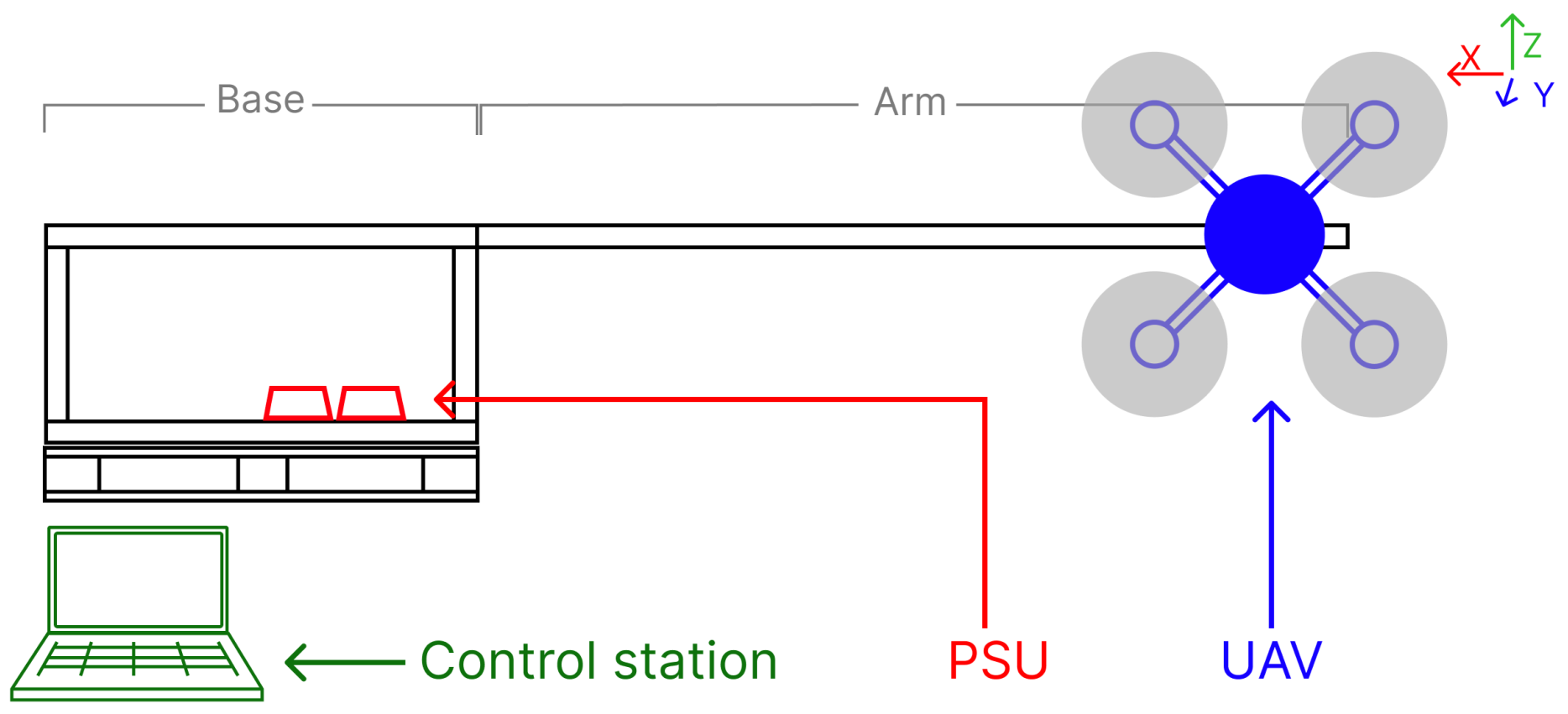
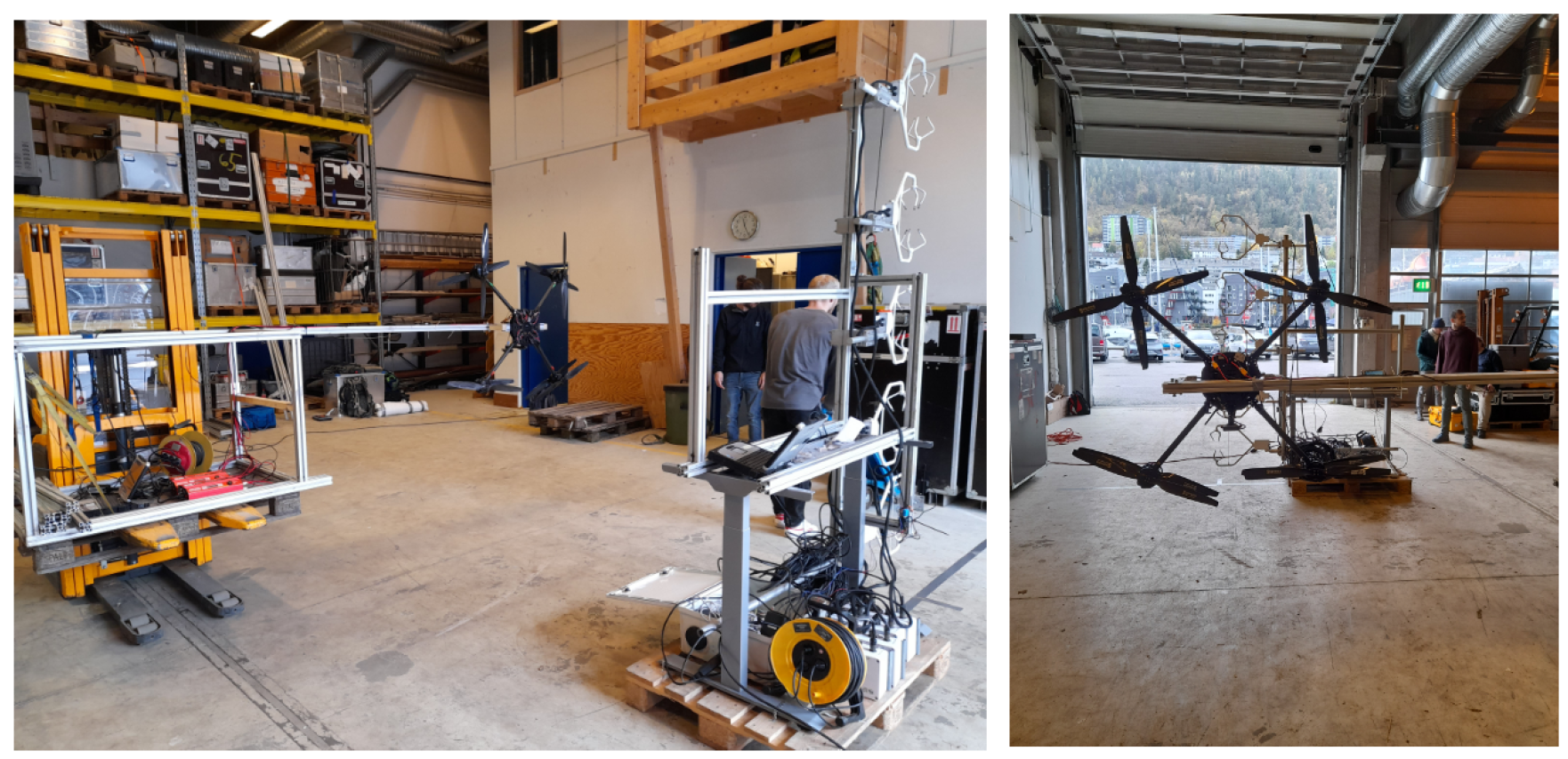
The mounting rack, sketched in Figure 2, consisted of a frame housing the ground control station (GCS), two power supplies units (PSU), and a horizontal extension arm holding the drone, placing its center away from the base. The rack was attached to a forklift, enabling both vertical and horizontal positioning upfront in the experiment. The UAV was oriented centrally towards the large bay door to direct the downwash out of the hall (see the right panel in Figure 3).Opening the door during the experiments allowed the far downwash to exit the enclosed hall volume, while the primary area of interest for our PIF measurements, a few rotor diameters beneath the drone, remained indoors, well shielded from external factors.
The fixed mounting of the drone during the experiments had additional benefits, including absolute stability for precise flow sensor positioning, continuous power from two SkyRC Technology eFUEL power supplies with a maximum output of 50 at 25 DC, and wired connection from a Panasonic TOUGHBOOK running Mission Planner GCS software (https://ardupilot.org/copter/docs/common-install-gcs.html) to the ArduPilot-based flight controller to regulate the throttle settings for the motors.
2.3. Sonic Anemometer Measurement Rig
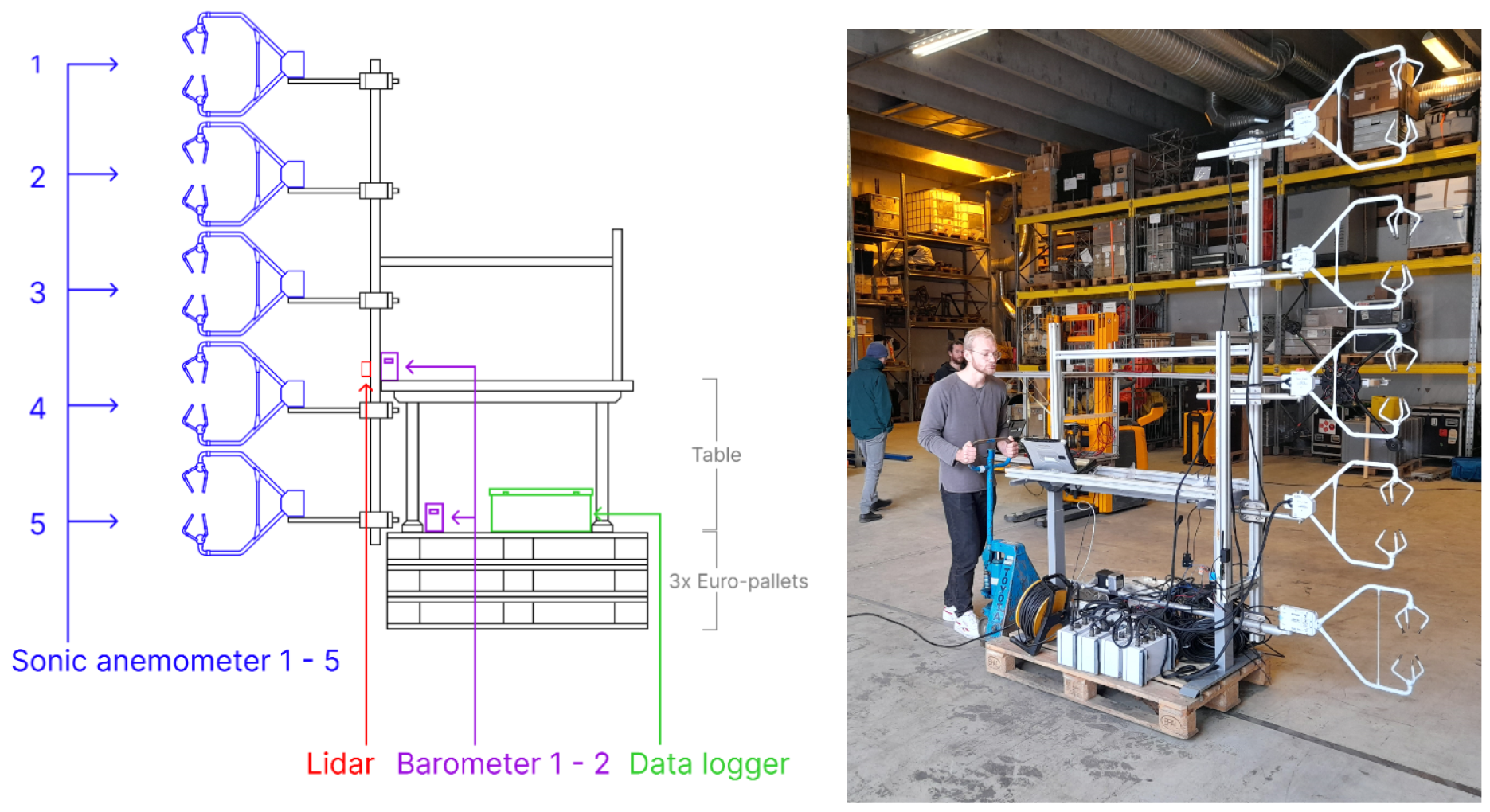
Five Campbell Scientific CSAT3 ultrasonic anemometers were used to measure the PIF. The anemometers were mounted to a mast with vertical spacing increments of , resulting in a measurement range from 0.60 to 2.70 above the ground. The mast was attached to the undercarriage of a height-adjustable table, allowing for an additional of vertical adjustment, extending the maximum measuring height to above ground. The whole measurement rig was then attached to a Euro-pallet and could thus be moved manually with a hydraulic jacklift (see also right panel in Figure 4). Each of the sonic anemometers sampled the 3D wind vector and the sonic temperature at a frequency of 10 and was connected to a Campbell Scientific CR3000 data logger for data storage and synchronization.
To associate velocity measurements to spatial points, distance measurements to a reference surface located at the respective wall of the hall perpendicular to the movement of the rig were taken using the Benewake TF02 LIDAR range finder. Those data were also recorded by the Campbell Scientific CR3000 data logger and thus exactly synchronized with the sonic anemometer data. The height of the sonic anemometers was noted down manually for each series of 2 D scans (see Section 4) and for redundancy, also measured by two barometers (one at a fixed level and one attached to the height-adjustable measurement mast). Both the LIDAR range finder and the two barometers were logged at a sampling frequency of 1 . The sensor assembly was placed on three Euro-pallets for mobility and the desired starting height. A schematic of the sensor setup is shown in Figure 4. Real-time data access and visualization were achieved using a Panasonic TOUGHBOOK running LoggerNet software (https://www.campbellsci.com/loggernet) and connected to the CR3000.
3. PIF Measurements
3.1. Measurement Pattern
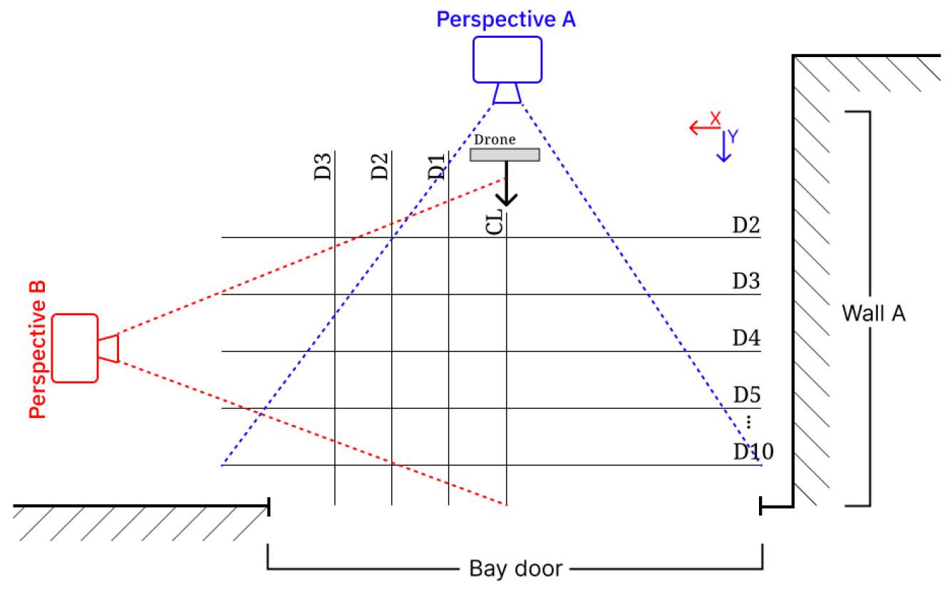
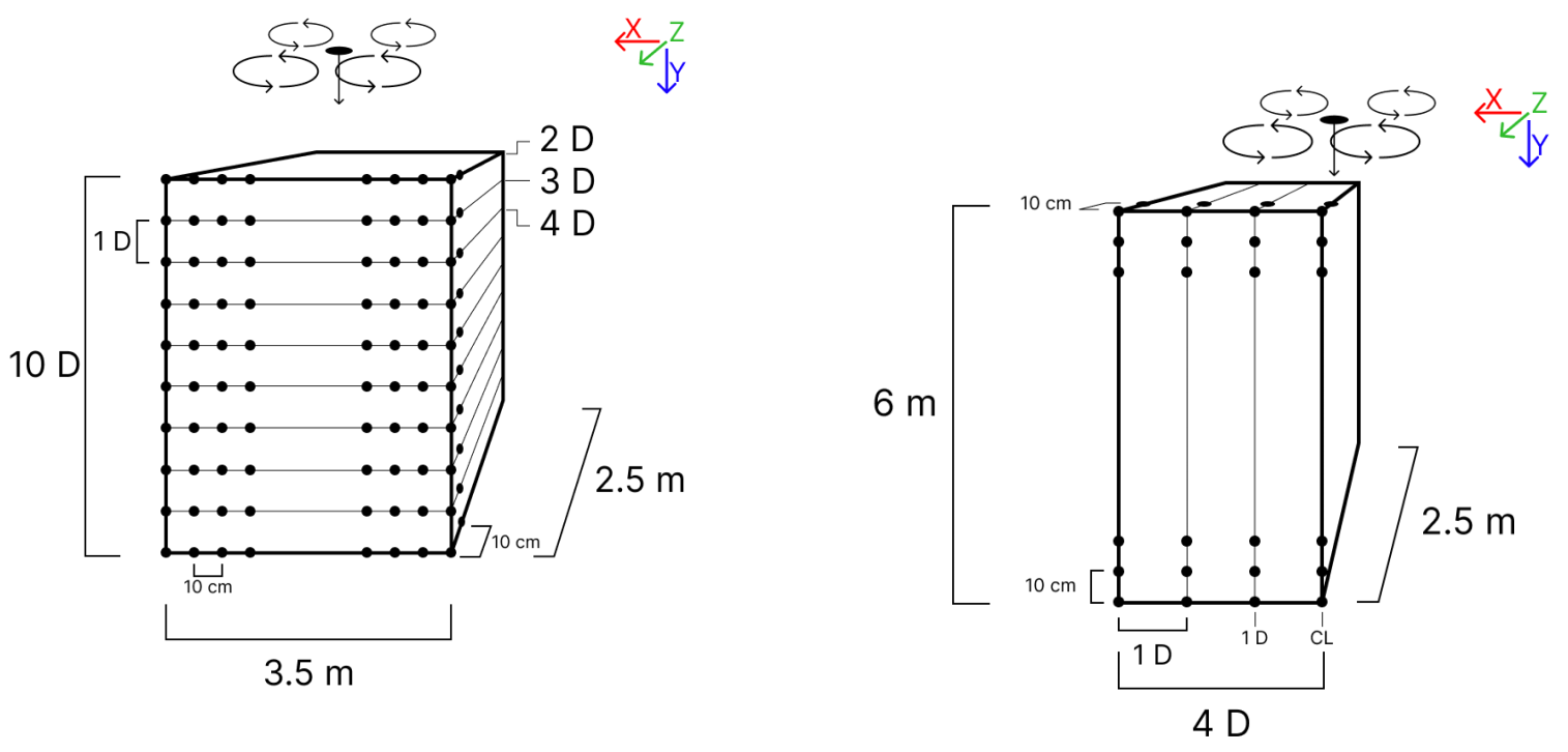
Figure 5 depicts the experimental coordinate system and its location in the hall. The z-axis is chosen to be normal to the floor, increasing with height above the hall surface. The downwash propagates along the y-axis in the positive direction, whereas the x-axis is parallel to the rotor plane, with the positive direction pointing away from Wall A. The measurement planes, designed to intersect the downwash across the x–z plane, were defined at intervals equivalent to the drone’s rotor diameter, D, of 71 cm. The first cross-section was placed at 2 D downstream from the rotor plane, the last one at 10 D. Additionally, measurement planes tangential to the downwash, spanning the y–z plane, were defined along the centerline of the downwash, i.e., , and at . All measurement planes cover the height interval between 0.60 to 3.10 above ground. The solid black lines in Figure 5 represent the chosen measurement pattern, each line corresponding to one x–z or y–z cross-section. At each cross-section, the array of anemometers was manually moved back and forth with a velocity in the order of ms−1 using a jacklift. For robust statistics, this measurement pattern was repeated 3 times for a given altitude setting of the height-adjustable table, thus sampling every point along the height of the 5 sonic anemometers 6 times. After that, the height-adjustable table was raised by , and the procedure was repeated until the whole cross-section was sampled in a vertical resolution of . Assuming quasi-stationary flow conditions, this measurement approach is expected to provide detailed insights into the average speed and structure of the drone downwash.
The entire measurement pattern was carried out for two different throttle settings of 35% and 45%, corresponding to a TOW of roughly 15 kg and 20 .
3.2. Data Processing
Upon the completion of data collection, two data sets were gathered. Data set 1 (DS1) contains all the velocity vectors , , and collected by the five sonic anemometers with a sampling frequency of 10 . The vectors , , and describe the measured wind speed relative to the coordinate system used for the experiment, where refers to the wind speed along the x-axis, along the y-axis, and perpendicular to the ground. The second data set (DS2), important for the exact localization of the flow measurements, contains the distance measurement to the relevant reference point and was gathered at 1 . The data were recorded over two days, the 24th and 25th of October 2022. In total, about 6 h of measurements resulted in 219,760 relevant wind velocity vectors in 10 resolution in DS1 for each of the 5 anemometers, corresponding to 21,976 spatial data points in DS2. To ensure the viability of the collected data points, the resulting data sets were first cleaned for missing data and physical outliers. The LiDAR distance measurements in DS2 contained several unphysical jumps and spikes. Considering that the data points were collected in a continuous and monotonous movement of a few cm s−1, all consecutive data points moving more than were dismissed and replaced by linearly interpolated values. For sequences of data points where the neighbors were also not deemed viable, a linear motion profile was fitted based on the start and end time and position of that corresponding pass. In DS2, 12% of data points were initially recorded as ‘not a number’ (NaN). The distribution of these measurements throughout the time series was uniform, displaying no discernible pattern in their occurrences. The cause behind this substantial number of faulty measurements remains unknown and can only be subject to speculation. However, after applying linear interpolation, the occurrence of NaN measurements decreased to zero.
Following the correction of the spatial data set, DS1 and DS2 were merged based on their recorded common timestamps. DS2 was linearly interpolated from the 1 original data onto the 10 resolution of DS1, resulting in a positioning of each wind measurement. The wind velocity vectors parallel to the motion of the anemometer assembly were adjusted by subtracting the calculated velocity of the assembly movement. For further analysis and interpretation, the flow measurements were now binned over spatial intervals. This results in two multi-dimensional arrays: one for the y–z cross-section and another for the x–z cross-section. Each two-dimensional array in the x–z plane spanned in the y-direction and in the z-direction, while in the arrays in the y–z plane spanned 6 in the x-direction and in the z-direction (Figure 6). Each matrix within these arrays represents a measurement plane, with each cell storing all velocity vectors captured over the corresponding spatial interval (Figure 6). On average, each cell contained about 35 velocity vectors. Each spatial cell was individually checked for velocity data outliers employing a 2.5 median absolute deviation threshold. This test identified, however, not a single exceedance of this threshold.
In the next step, the mean velocity and mean velocity variance were calculated for each cell. The cell-averaged mean PIF was estimated as the magnitude of the mean velocity vector of that cell using
The PIF variability of each cell was estimated using turbulent kinetic energy (TKE) per unit mass calculated using the following equation:
applying cell-wise Reynolds decomposition,
with .
4. Results and Discussion
4.1. Mean PIF
For the x–z measurement planes, the perspective of the plotted results is looking from the UAV along the y-axis downstream through the relevant plane, as indicated by “Perspective A” in Figure 5. Conversely, for the y–z measurement planes, the perspective is looking at the downwash along the x-axis from a location of positive x-value, as indicated by “Perspective B” in Figure 5, i.e., representing cross-sections of the main downwash at different distances from the center line of the drone.
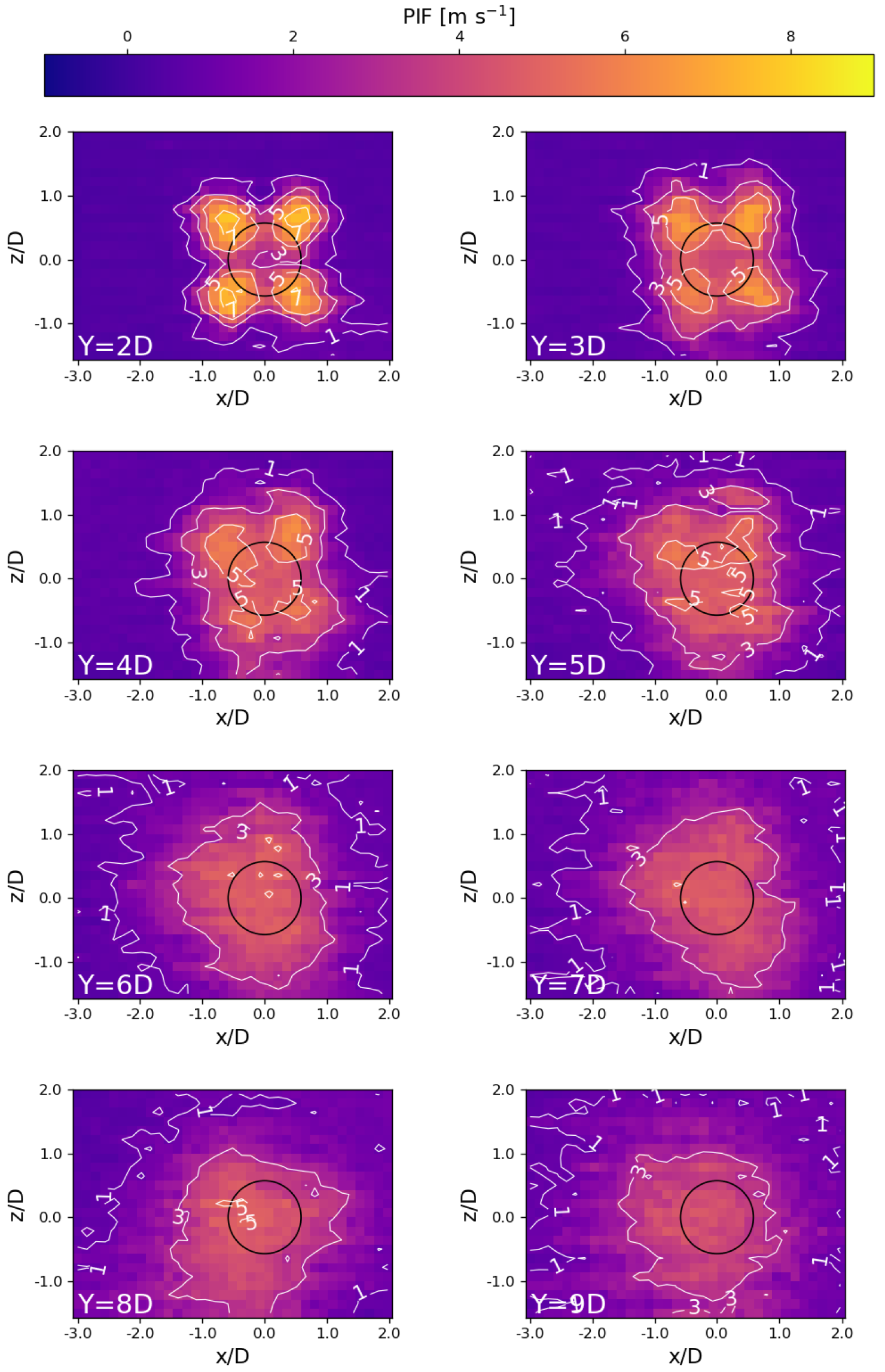
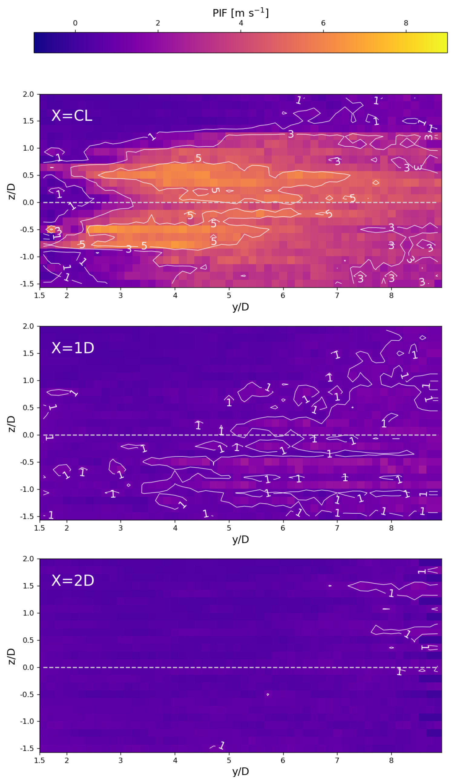
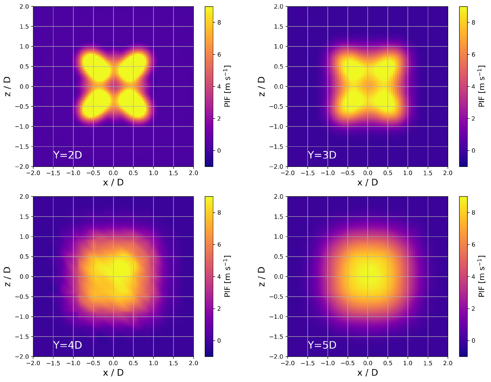
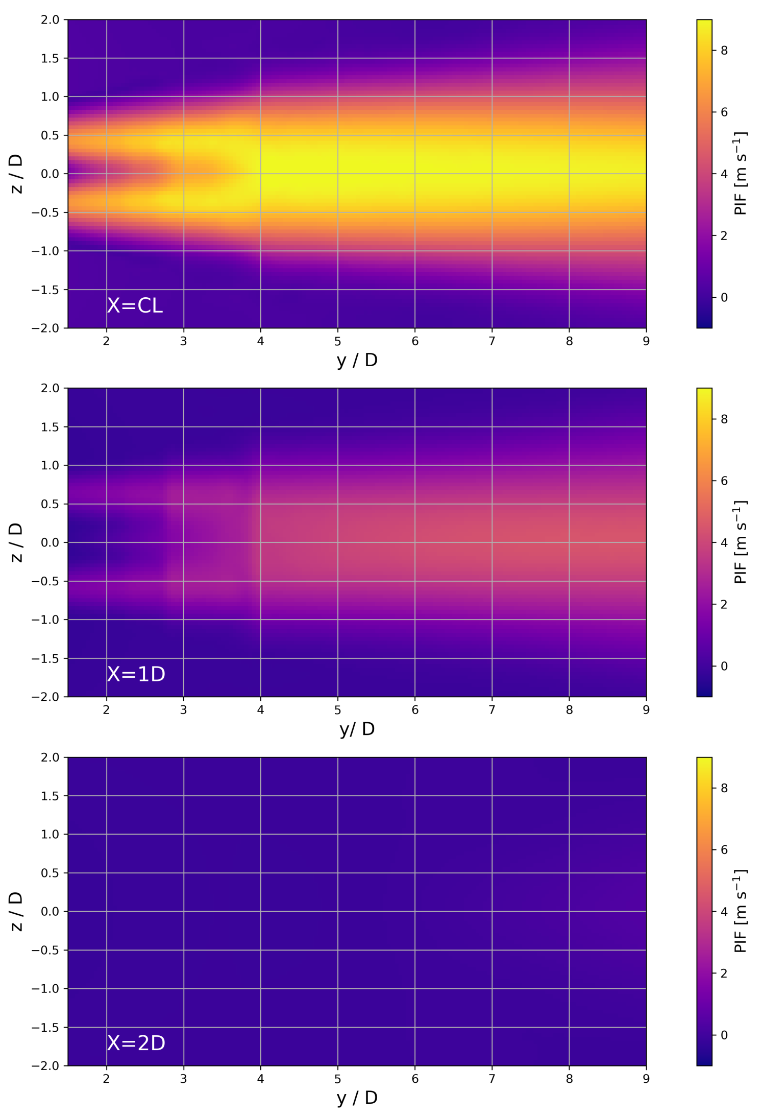
Visualizing the matrices within these tensors as heat maps, we obtain a good visual representation of the PIF produced by the drone as it propagates downstream. In these visualizations, the PIF corresponds to the cell-averaged velocity magnitude (Equation (1)), where brighter colors denote higher values. The depicted results, showcased in Figure 7 and Figure 8, illustrate the progression of the PIF for a throttle setting of 35 %. Figure 7 depicts the mean PIF measured across the x–z planes, employing “Perspective A” in Figure 5. These planes are set at increments of one rotor diameter, beginning at a distance of two rotor diameters downstream of the mean rotor plane, , and extending to . Figure 8 depicts the y–z planes, parallel to the main downwash direction seen from “Perspective B” in Figure 5. The first plane is at the center line (CL, at ) of the UAV, and subsequent planes are measured at and from the center. Each colored cell in both figures corresponds to a 10 by 10 cm cell within their respective matrices.
The development of the PIF can be characterized as follows:
- Distinct hotspots of high PIF are clearly visible, one for each rotor set. The peak velocities within the range of 6 ms−1 to 7 ms−1 are observed at the center of the four hotspots. Beyond a distance equivalent to rotor diameter in x- or z-direction from the drone’s center, there is no substantial observed flow disturbance.
- The initially distinct hotspots begin to converge, forming a more consolidated and uniform downwash structure. The region with the highest velocities is centered behind the drone, with peak velocities of 5 ms−1 to 6 ms−1 for a throttle setting of 35%. The data indicate a more pronounced onset of downwash expansion at this stage. The figures also show that the air between the downwash and the floor starts to speed up.
- The hotspots corresponding to the four-rotor sets have now completely dissipated. The downwash center, marked by the region of greatest velocities, remains largely centered relative to the drone. Notably, the downwash starts to expand asymmetrically, indicating the potential effect of walls, floors, and ceilings in the far flow of the downwash.
- At this stage, the downwash center has shifted towards the left by about . Peak velocities around 4 ms−1 were observed. The edges of the downwash lean more towards the bottom left.
It is worth noting here that both the acceleration of the air under the downwash at a y-position of to and the predominant expansion of the downwash in the negative x-direction, can likely be attributed to the specifics of the test setup and the available space. The asymmetric expansion of the downwash in the z-direction is probably a consequence of the drone not being mounted at a sufficient height, leading to air acceleration between the ground and the downwash. The expansion of the downwash in the negative y-direction is most likely a result of inflow through the bay door, driven by the need to maintain mass equilibrium as the drone displaces air out of the confined space through the bay door. Qualitative measurements of this compensation flow were conducted, indicating its presence but not exactly quantifying its strength and extension.
4.2. PIF Variabillity
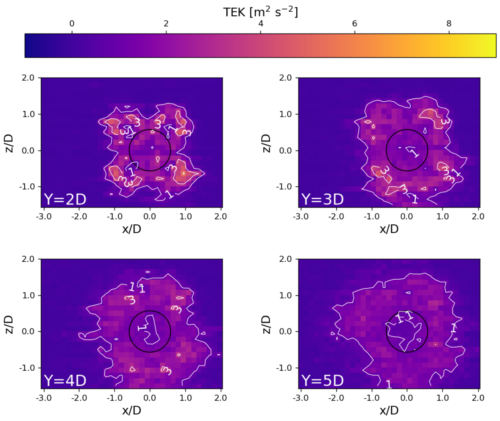
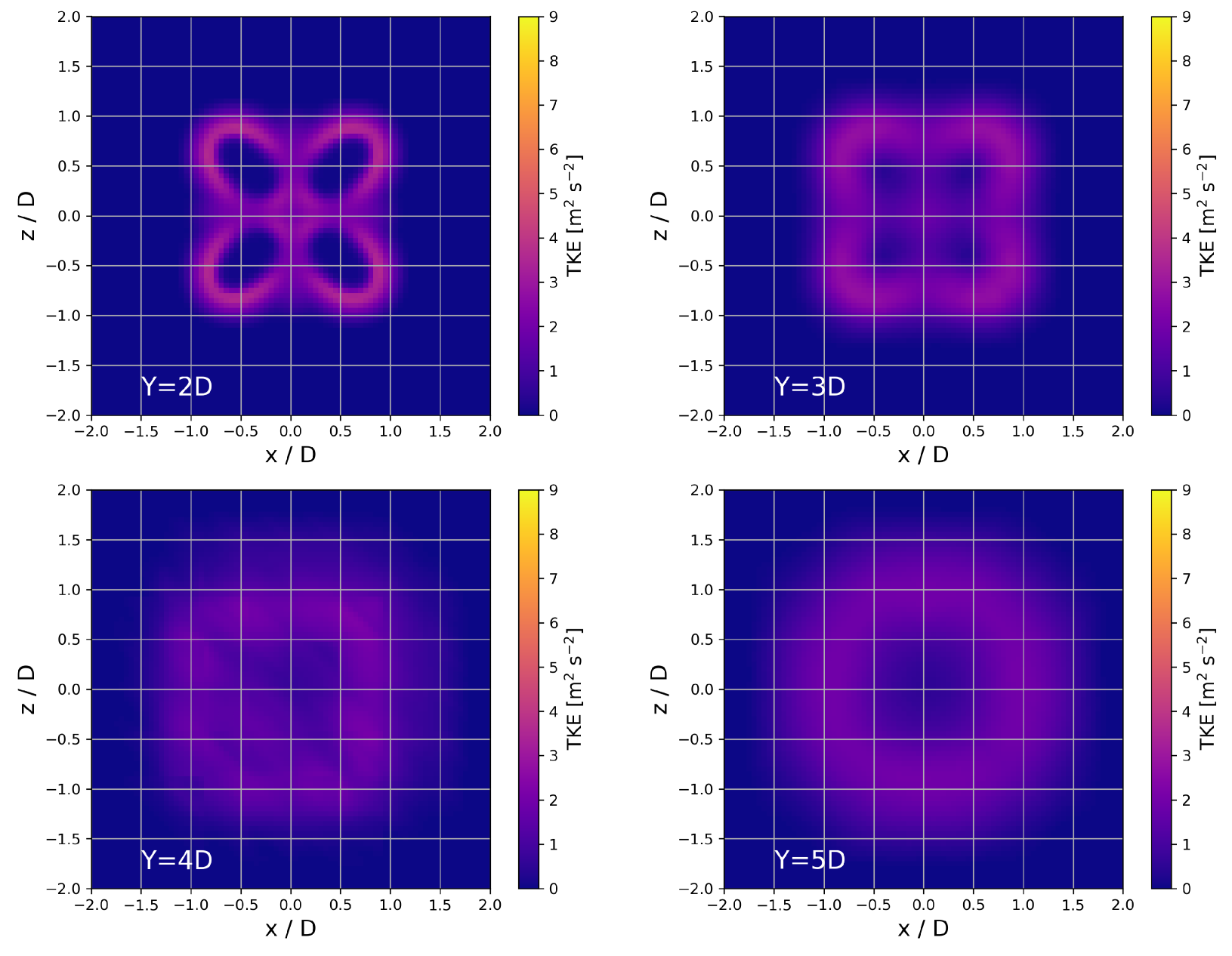
Observing the trends discerned from the results thus far and keeping in mind that the primary area of interest for sensor placement of a boom-mounted wind sensor is within the first few D downstream of the rotor plane, the PIF effect on the flow will be analyzed by TKE cross-sections up to a downstream distance of (Figure 9).
The results demonstrate that the region with the most significant variability in PIF lies at the interface where the faster-moving downwash meets the stagnant surrounding air, i.e., the area with the strongest velocity shear. It is also important to highlight that the variations in PIF are predominantly concentrated within the downwash region. This underpins the idea that a substantial portion of PIF disturbance for a boom-mounted sonic anemometer can be effectively mitigated by citing the sensor below the rotor plane at a distance of 1D to 2D away from the drone’s center.
4.3. Comparison with CFD Simulations and Environmental Observations
One main motivation for the low-cost experiment presented in this study was to provide a first evaluation of the realism of CFD simulations for the modeling of PIF of our chosen multicopter setup. Corresponding simulations for this system, with a focus on wind sensor placement, have recently been performed by [49].
4.3.1. CFD Simulations
The simulations presented and discussed in the following have been performed by Ansys Fluent. It must be noted that the actual geometry of the drone is simplified, e.g., by assuming an actuator disc instead of rotating propellers [50,51,52], and neglecting the body of the drone. Thus, the drone is represented by eight two-dimensional discs that create an instantaneous pressure jump in the flow. In the simulation, the domain is a cube with each side measuring . Within this cubic domain, the drone is modeled with its rotors plane oriented horizontally, ensuring that the downwash is directed vertically downward. The drone is positioned precisely in the horizontal center of the cube, equidistant at from each side wall. Vertically, it is placed slightly towards the top, from the ceiling and from the bottom, allowing for ample space for airflow and downwash development. To enhance the stability and convergence of the solution, the top surface of the cube is defined with an inlet velocity of ms−1. Conversely, the opposite face at the bottom is designated as a pressure outlet. Results are rotated to align with the experimental measurements’ reference frame, and PIF values are refined by subtracting the background flow.
Figure 10 shows the resulting vertical velocities in the downwash modeled at different distances below the drone. The distances presented are chosen in accordance with the upper four panels in Figure 7. The modeled vertical velocities are, in general, higher (max. values of around 9 ms−1 for a distance of ) than our measurements in the hall (max. around 7 ms−1). This might mainly be explained by the simplified representation of the drone in the model simulations, in particular, the intrinsic uncertainty in relating the chosen throttle setting for the drone motors in the experiment to an exact value of the instantaneous pressure jump of the actuator discs in the CFD simulations. In addition, the flow is simulated with a constant background turbulence of 5 %, a value that might underestimate ambient turbulence conditions. Despite this difference in the flow magnitude, it compares the structure and dimension of the downwash between the model and measurement very well. Both identify four clearly separated downwash areas at distances of and . The slightly elliptical shape is caused by the tilt angle of 8° for the propellers of our Foxtech drone, which is also implemented as a corresponding tilt of the actuator discs in the CFD. For distances beyond , the individual downwash centers have clearly merged into a single, large, and rather homogenous downwash zone.
The general overestimation in the downwash velocity described above can also be seen in the comparison of the cross-sections along the y–z plane along the center line of the drone (upper panels in Figure 8 for the measurements and Figure 11 for the CFD simulations). The consecutive cross-section at distance shows a fast decrease of the downwash effect that has nearly fully disappeared at . The width of the downwash area and its structure are rather similar. Some minor differences observed in the experiment can be associated with the interaction of the downwash with the floor of the hall at the lower boundary and the observed counterflow entering the open bay door close to the ceiling, inhibiting the widening of the downwash at the top.
Figure 12 shows the TKE output of the CFD simulations in the x–z plane for distances from the rotor plane between and . The absolute values correspond well with the measurements in magnitude, although it must be kept in mind that they are calculated in two different ways. The measured values presented in Figure 9 are based on the velocity variances for each spatial bin following Equation (2), while the simulated ones represent the solution of the steady-state simulations of the CFD code based on the k- model. The TKE from the model simulations is, in particular, closer to the rotor plane and considerably sharper concentrated, indicating a lower diffusion in the model compared to the flow in our laboratory measurements. However, there are a few striking and interesting similarities that can be highlighted. The first is the transition from four slightly elliptical and clearly separated areas of enhanced TKE at below the rotor plane into a single and rather homogeneous donut-shaped TKE structure at . The second is related to the detailed structure of the four areas of enhanced TKE at a distance of , where both simulation and the measurements indicate a varying level of TKE along the ellipse, with the corresponding maximum values towards the outer edges.
4.3.2. Outdoor Observations
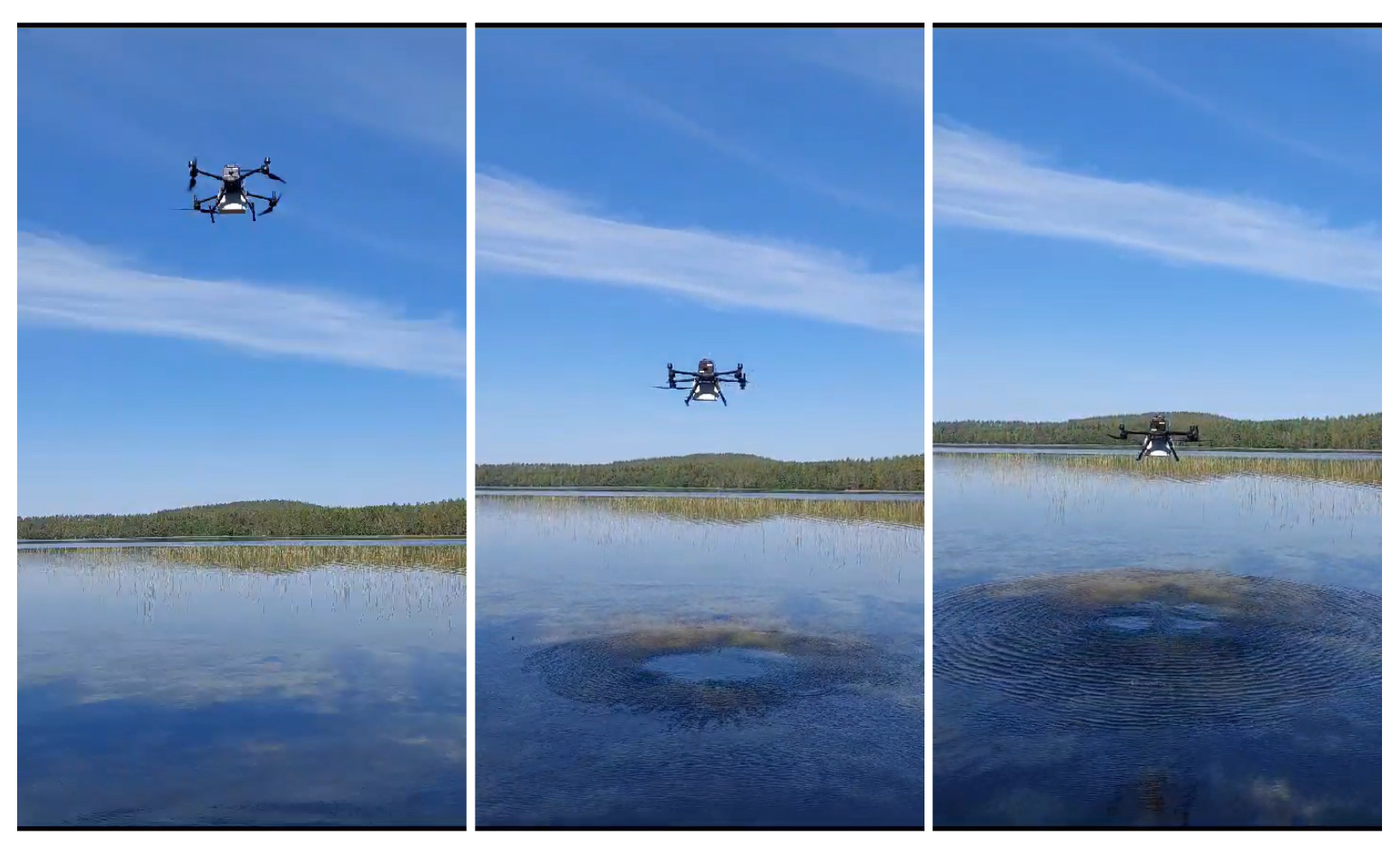
Another possibility of a qualitative comparison and validation of our measurement results arises from a visualization of the PIF of a hovering multi-rotor drone over a calm water surface in low-wind conditions. Figure 13 shows three consecutive still pictures extracted from a video of a slowly descending drone above a lake. At heights above , the downwash at the surface is not strong enough to create any visual disturbance (picture to the left). Closer to the surface, visualized in the picture in the center for a height of , a clear single central downwash appears, surrounded by a ring of small surface waves indicating the flow divergence in the outflow region. At a level of around , the single downwash quickly transforms into four separated downwash zones created by the individual propellers (picture to the right). Although created by rather different drone systems (the Foxtech D130 octocopter in X8 configuration for the laboratory tests and the DJI Matrice 300 RTK quadcopter hovering over the lake), the resulting flows show quite intriguing similarities that indicate a considerable degree of generality in the PIF created by a drone with four centers of rotation. The most prominent one is the transformation of the individual rotor flows to one combined downwash flow area, occurring in a distance of approximately below the rotor plane, in good agreement with both our measurements and the CFD simulations.
5. Conclusions
Given the need to understand how drone systems affect the surrounding air to ensure optimal sensor placement and the lack of an adequate wind tunnel facility at hand, this paper has shown that there are ways to obtain the desired measurements and information on a shoestring budget. The described approach of tilting the drone by 90 degree and measuring the now horizontal downwash with a rig of five sonic anemometers in cross-sections in various distances perpendicular and parallel to the downwash direction has shown that it is possible to obtain reliable and realistic measurements of the PIF generated by the drone. Some distortions in the results were observed at locations further away from the rotor plane, which can be attributed to the specific constraints of the available experimental indoor space. Despite those unavoidable constraints and the implied potential interactions with ceilings, walls, and floors, we are confident that the approach of conducting the experiment in a controlled environment poses more advantages than backdraws.
The data obtained from this experiment corroborated the results obtained from precursory CFD simulations Ghirardelli et al. [49]. The characteristics of the experimental results matched well with the characteristics of the simulations, even though the conditions of the two environments differed slightly. An observed overestimation of the CFD modeled downwash velocities in the order of 20% can be mainly attributed to the uncertain relationship between the throttle setting of the drone and the chosen pressure jump prescribed at the location of the actuator discs in the CFD simulations. With respect to our sensor placement considerations, this overestimation indicates that following the CFD simulations will provide a rather conservative approach to the flow disturbances created by the PIF.
The retrieved dataset can serve as an expansion of the existing foundation to be used for future analysis and comparison with other model simulations, e.g., in combination with a complementary experimental dataset of high-resolution, in-flight measurements of the drone downwash of the Foxtech D130 X8 drone by a short-range LiDAR WindScanner system described by Jin et al. [53].
The combination of CFD simulations with targeted measurements provides, in our opinion, a reliable and cost-efficient framework to address the topic of optimal sensor placement on multi-rotor drones. Simulations can be efficiently performed for many drone configurations and environmental flight conditions, thus identifying potential sweet spots for the sensor mounting. Those areas have then to be investigated in more detail by corresponding high-quality measurements.
Author Contributions
Conceptualization, A.A.F., M.G., S.T.K. and J.R.; methodology, A.A.F., M.G., S.T.K., T.O.K. and J.R.; software, A.A.F., M.G., S.T.K. and E.C.; formal analysis, A.A.F., M.G. and S.T.K.; resources, M.G., S.T.K. and J.R.; data curation, A.A.F., M.G. and J.R.; writing—original draft preparation, A.A.F., M.G., S.T.K., E.C. and J.R.; writing—review and editing, A.A.F., M.G., S.T.K., E.C., T.O.K. and J.R.; visualization, A.A.F., M.G., S.T.K., E.C. and J.R.; supervision, M.G., S.T.K. and J.R.; project administration, J.R. and S.T.K.; funding acquisition, J.R. and S.T.K. All authors have read and agreed to the published version of the manuscript.
Funding
Parts of this research was funded by the European Union Horizon 2020 research and innovation program as part of the Marie Skłodowska-Curie Innovation Training Network Train2Wind (grant no. 861291;https://www.train2wind.eu/, last access: 13 October 2023).
Institutional Review Board Statement
Not applicable.
Informed Consent Statement
Not applicable.
Data Availability Statement
The data are available from the corresponding author upon request due to time issue. The data presented in this study are now prepared for publication in an open data repository. Until then they are available on request from the corresponding author.
Acknowledgments
Many thanks to our institute engineers Anak Bhandari, Helge Bryhni, and Tor de Lange for their help and assistance in preparing the measurement setup and accepting the several-day blockage of our storage hall at Marinoholmen for the experiment. The authors are also very grateful to Alizee Lehoux from Uppsala University for the provision of the video material of a hovering drone that formed the basis for Figure 13 in the manuscript.
Conflicts of Interest
The authors declare no conflict of interest. The funders had no role in the design of the study, in the collection, analyses, or interpretation of data, in the writing of the manuscript, or in the decision to publish the results.
Abbreviations
The following abbreviations are used in this manuscript:
| ABL | atmospheric boundary layer |
| CFD | computational fluid dynamic |
| GCS | ground control station |
| PIF | propeller-induced flow |
| PSU | power supply unit |
| RPAS | remotely piloted aircraft system |
| TKE | turbulent kinetic energy |
| TOW | take-off weight |
| UAS | uncrewed aerial system |
| UAV | uncrewed aerial vehicle |
References
- Stull, R.B. An Introduction to Boundary Layer Meteorology; Springer: Dordrecht, The Netherlands, 1988. [Google Scholar]
- Wyngaard, J.C. Turbulence in the Atmosphere; Cambridge University Press: Cambridge, UK, 2010. [Google Scholar]
- Jensen, N.; Hjort-Hansen, E. Turbulence and Response Measurements at the Sotra Bridge: Dynamic Excitation of Structures by Wind; Report No. STF71 A; SINTEF: Trondheim, Norway, 1977; Volume 78003. [Google Scholar]
- Kristensen, L.; Jensen, N. Lateral coherence in isotropic turbulence and in the natural wind. Bound.-Layer Meteorol. 1979, 17, 353–373. [Google Scholar] [CrossRef]
- Kaimal, J.C.; Wyngaard, J.; Izumi, Y.; Coté, O. Spectral characteristics of surface-layer turbulence. Q. J. R. Meteorol. Soc. 1972, 98, 563–589. [Google Scholar]
- Jensen, N.O. Simultaneous measurements of turbulence over land and water. Bound.-Layer Meteorol. 1978, 15, 95–108. [Google Scholar] [CrossRef]
- Mauder, M.; Foken, T.; Aubinet, M.; Ibrom, A. Eddy-Covariance Measurements. In Springer Handbook of Atmospheric Measurements; Foken, T., Ed.; Springer: Cham, Switzerland, 2021; Chapter 55. [Google Scholar]
- Mahrt, L. Stably Stratified Atmospheric Boundary Layers. Annu. Rev. Fluid Mech. 2014, 46, 23–45. [Google Scholar] [CrossRef]
- Kral, S.T.; Reuder, J.; Vihma, T.; Suomi, I.; Haualand, K.F.; Urbancic, G.H.; Greene, B.R.; Steeneveld, G.J.; Lorenz, T.; Maronga, B.; et al. The Innovative Strategies for Observations in the Arctic Atmospheric Boundary Layer Project (ISOBAR): Unique Finescale Observations under Stable and Very Stable Conditions. Bull. Am. Meteorol. Soc. 2021, 102, E218–E243. [Google Scholar] [CrossRef]
- Porté-Agel, F.; Bastankhah, M.; Shamsoddin, S. Wind-Turbine and Wind-Farm Flows: A Review. Bound.-Layer Meteorol. 2020, 174, 1–59. [Google Scholar] [CrossRef] [PubMed]
- Veers, P.; Dykes, K.; Lantz, E.; Barth, S.; Bottasso, C.L.; Carlson, O.; Clifton, A.; Green, J.; Green, P.; Holttinen, H.; et al. Grand challenges in the science of wind energy. Science 2019, 366, eaau2027. [Google Scholar] [CrossRef] [PubMed]
- Mikkelsen, T.; Sjöholm, M.; Angelou, N.; Mann, J. 3D WindScanner lidar measurements of wind and turbulence around wind turbines, buildings and bridges. In Proceedings of the IOP Conference Series: Materials Science and Engineering; IOP Publishing: Bristol, UK, 2017; Volume 276, p. 012004. [Google Scholar]
- Cheynet, E.; Flügge, M.; Reuder, J.; Jakobsen, J.B.; Heggelund, Y.; Svardal, B.; Saavedra Garfias, P.; Obhrai, C.; Daniotti, N.; Berge, J.; et al. The COTUR project: Remote sensing of offshore turbulence for wind energy application. Atmos. Meas. Tech. 2021, 14, 6137–6157. [Google Scholar] [CrossRef]
- Ogawa, Y.; Ohara, T. Observation of the turbulent structure in the planetary boundary layer with a kytoon-mounted ultrasonic anemometer system. Bound.-Layer Meteorol. 1982, 22, 123–131. [Google Scholar] [CrossRef]
- Hobby, M.J. Turbulence Measurements from a Tethered Balloon. Ph.D. Thesis, University of Leeds, Leeds, UK, 2013. [Google Scholar]
- Canut, G.; Couvreux, F.; Lothon, M.; Legain, D.; Piguet, B.; Lampert, A.; Maurel, W.; Moulin, E. Turbulence fluxes and variances measured with a sonic anemometer mounted on a tethered balloon. Atmos. Meas. Tech. 2016, 9, 4375–4386. [Google Scholar] [CrossRef]
- Blanc, T.V.; Plant, W.J.; Keller, W.C. The Naval Research Laboratory’s Air-Sea Interaction Blimp Experiment. Bull. Am. Meteorol. Soc. 1989, 70, 354–365. [Google Scholar] [CrossRef]
- Nambiar, M.K.; Byerlay, R.A.E.; Nazem, A.; Nahian, M.R.; Moradi, M.; Aliabadi, A.A. A Tethered Air Blimp (TAB) for observing the microclimate over a complex terrain. Geosci. Instrum. Methods Data Syst. 2020, 9, 193–211. [Google Scholar] [CrossRef]
- Elston, J.; Argrow, B.; Stachura, M.; Weibel, D.; Lawrence, D.; Pope, D. Overview of small fixed-wing unmanned aircraft for meteorological sampling. J. Atmos. Ocean. Technol. 2015, 32, 97–115. [Google Scholar] [CrossRef]
- Pinto, J.O.; O’Sullivan, D.; Taylor, S.; Elston, J.; Baker, C.B.; Hotz, D.; Marshall, C.; Jacob, J.; Barfuss, K.; Piguet, B.; et al. The Status and Future of Small Uncrewed Aircraft Systems (UAS) in Operational Meteorology. Bull. Am. Meteorol. Soc. 2021, 102, E2121–E2136. [Google Scholar] [CrossRef]
- de Boer, G.; Argrow, B.; Cassano, J.; Cione, J.; Frew, E.; Lawrence, D.; Wick, G.; Wolff, C. Advancing Unmanned Aerial Capabilities for Atmospheric Research. Bull. Am. Meteorol. Soc. 2019, 100, ES105–ES108. [Google Scholar] [CrossRef]
- Båserud, L.; Reuder, J.; Jonassen, M.O.; Kral, S.T.; Paskyabi, M.B.; Lothon, M. Proof of concept for turbulence measurements with the RPAS SUMO during the BLLAST campaign. Atmos. Meas. Tech. 2016, 9, 4901–4913. [Google Scholar] [CrossRef]
- Mansour, M.; Kocer, G.; Lenherr, C.; Chokani, N.; Abhari, R.S. Seven-Sensor Fast-Response Probe for Full-Scale Wind Turbine Flowfield Measurements. J. Eng. Gas Turbines Power 2011, 133, 081601. [Google Scholar] [CrossRef]
- Calmer, R.; Roberts, G.C.; Preissler, J.; Sanchez, K.J.; Derrien, S.; O’Dowd, C. Vertical wind velocity measurements using a five-hole probe with remotely piloted aircraft to study aerosol–cloud interactions. Atmos. Meas. Tech. 2018, 11, 2583–2599. [Google Scholar] [CrossRef]
- Alaoui-Sosse, S.; Durand, P.; Medina, P.; Pastor, P.; Lothon, M.; Cernov, I. OVLI-TA: An Unmanned Aerial System for Measuring Profiles and Turbulence in the Atmospheric Boundary Layer. Sensors 2019, 19, 581. [Google Scholar] [CrossRef]
- Witte, B.; Singler, R.; Bailey, S. Development of an Unmanned Aerial Vehicle for the Measurement of Turbulence in the Atmospheric Boundary Layer. Atmosphere 2017, 8, 195. [Google Scholar] [CrossRef]
- Wildmann, N.; Hofsäß, M.; Weimer, F.; Joos, A.; Bange, J. MASC—A small Remotely Piloted Aircraft (RPA) for wind energy research. Adv. Sci. Res. 2014, 11, 55–61. [Google Scholar] [CrossRef]
- Wildmann, N.; Ravi, S.; Bange, J. Towards higher accuracy and better frequency response with standard multi-hole probes in turbulence measurement with remotely piloted aircraft (RPA). Atmos. Meas. Tech. 2014, 7, 1027–1041. [Google Scholar] [CrossRef]
- Lenschow, D.H.; Spyers-Duran, P. Research Aviation Facility Bulletin 23: Measurement Techniques, Air Motion Sensing; NCAR: Broomfield, CO, USA, 1989. [Google Scholar]
- Crawford, T.L.; McMillen, R.T.; Dobosy, R.J.; MacPherson, I. Correcting airborne flux measurements for aircraft speed variation. Bound.-Layer Meteorol. 1993, 66, 237–245. [Google Scholar] [CrossRef]
- Drüe, C.; Heinemann, G. A Review and Practical Guide to In-Flight Calibration for Aircraft Turbulence Sensors. J. Atmos. Ocean. Technol. 2013, 30, 2820–2837. [Google Scholar] [CrossRef]
- Vellinga, O.S.; Dobosy, R.J.; Dumas, E.J.; Gioli, B.; Elbers, J.a.; Hutjes, R.W.a. Calibration and quality assurance of flux observations from a small research aircraft. J. Atmos. Ocean. Technol. 2013, 30, 161–181. [Google Scholar] [CrossRef]
- Davenport, A.G. The response of slender, line-like structures to a gusty wind. Proc. Inst. Civ. Eng. 1962, 23, 389–408. [Google Scholar] [CrossRef]
- Shimura, T.; Inoue, M.; Tsujimoto, H.; Sasaki, K.; Iguchi, M. Estimation of Wind Vector Profile Using a Hexarotor Unmanned Aerial Vehicle and Its Application to Meteorological Observation up to 1000 m above Surface. J. Atmos. Ocean. Technol. 2018, 35, 1621–1631. [Google Scholar] [CrossRef]
- Hofsäß, M.; Bergmann, D.; Denzel, J.; Cheng, P.W. Flying UltraSonic—A new way to measure the wind. Wind Energy Sci. Discuss. 2019, 1–21. [Google Scholar] [CrossRef]
- Thielicke, W.; Hübert, W.; Müller, U.; Eggert, M.; Wilhelm, P. Towards accurate and practical drone-based wind measurements with an ultrasonic anemometer. Atmos. Meas. Tech. 2021, 14, 1303–1318. [Google Scholar] [CrossRef]
- Bailey, S.C.C.; Sama, M.P.; Canter, C.A.; Pampolini, L.F.; Lippay, Z.S.; Schuyler, T.J.; Hamilton, J.D.; MacPhee, S.B.; Rowe, I.S.; Sanders, C.D.; et al. University of Kentucky measurements of wind, temperature, pressure and humidity in support of LAPSE-RATE using multisite fixed-wing and rotorcraft unmanned aerial systems. Earth Syst. Sci. Data 2020, 12, 1759–1773. [Google Scholar] [CrossRef]
- McConville, A.; Richardson, T. High-altitude vertical wind profile estimation using multirotor vehicles. Front. Robot. AI 2023, 10, 1112889. [Google Scholar] [CrossRef]
- Li, Z.; Pu, O.; Pan, Y.; Huang, B.; Zhao, Z.; Wu, H. A Study on Measuring the Wind Field in the Air Using a Multi-rotor UAV Mounted with an Anemometer. Bound.-Layer Meteorol. 2023, 187, 1–27. [Google Scholar] [CrossRef]
- Prudden, S.; Fisher, A.; Mohamed, A.; Watkins, S. A flying anemometer quadrotor: Part 1. In Proceedings of the 7th International Micro Air Vehicle Conference and Competition—Past, Present and Future, Toulouse, France, 18–21 September 2017. [Google Scholar]
- Fabrizio Schiano, J.A.M. Towards Estimation and Correction of Wind Effects on a Quadrotor UAV. In Proceedings of the 2014 International Micro Air Vehicle Conference and Competition—Past, Present and Future, Delft, The Netherlands, 12–15 August 2014. [Google Scholar]
- Paz, C.; Suárez, E.; Gil, C.; Vence, J. Assessment of the methodology for the CFD simulation of the flight of a quadcopter UAV. J. Wind Eng. Ind. Aerodyn. 2021, 218, 104776. [Google Scholar] [CrossRef]
- Deters, R.W.; Krishnan, G.K.A.; Selig, M.S. Reynolds number effects on the performance of small-scale propellers. In Proceedings of the 32nd AIAA Applied Aerodynamics Conference, Atlanta, GA, USA, 16–20 June 2014. [Google Scholar]
- Kutty, H.A.; Rajendran, P. 3D CFD Simulation and Experimental Validation of Small APC Slow Flyer Propeller Blade. Aerospace 2017, 4, 10. [Google Scholar] [CrossRef]
- Zheng, Y.; Yang, S.; Liu, X.; Wang, J.; Norton, T.; Chen, J.; Tan, Y. The computational fluid dynamic modeling of downwash flow field for a six-rotor UAV. Front. Agric. Sci. Eng. 2018, 5, 159–167. [Google Scholar] [CrossRef]
- Guo, Q.; Zhu, Y.; Tang, Y.; Hou, C.; He, Y.; Zhuang, J.; Zheng, Y.; Luo, S. CFD simulation and experimental verification of the spatial and temporal distributions of the downwash airflow of a quad-rotor agricultural UAV in hover. Comput. Electron. Agric. 2020, 172, 105343. [Google Scholar] [CrossRef]
- Guillermo, P.P.H.; Daniel, A.M.V.; Eduardo, G.G.E. CFD Analysis of Two and Four Blades for Multirotor Unmanned Aerial Vehicle. In Proceedings of the 2018 IEEE 2nd Colombian Conference on Robotics and Automation (CCRA), Barranquilla, Colombia, 1–3 November 2018; pp. 1–6. [Google Scholar] [CrossRef]
- Lei, Y.; Lin, R. Effect of wind disturbance on the aerodynamic performance of coaxial rotors during hovering. Meas. Control 2019, 52, 665–674. [Google Scholar] [CrossRef]
- Ghirardelli, M.; Kral, S.T.; Müller, N.C.; Hann, R.; Cheynet, E.; Reuder, J. Flow Structure around a Multicopter Drone: A Computational Fluid Dynamics Analysis for Sensor Placement Considerations. Drones 2023, 7, 467. [Google Scholar] [CrossRef]
- Rankine, W.J.M. On the mechanical principles of the action of propellers. Trans. Inst. Nav. Archit. 1865, 6, 13–39. [Google Scholar]
- Froude, R.E. On the part played in propulsion by differences of fluid pressure. Trans. Inst. Nav. Archit. 1889, 30, 390. [Google Scholar]
- Sayigh, A. Comprehensive Renewable Energy; Elsevier: Amsterdam, The Netherlands, 2012; Volume 2. [Google Scholar]
- Jin, L.; Ghirardelli, M.; Mann, J.; Sjöholm, M.; Kral, S.T.; Reuder, J. Rotary-wing drone-induced flow—Comparison of simulations with lidar measurements. EGUsphere 2023. preprint. [Google Scholar] [CrossRef]
Figure 1.
Image of the rotary-wing UAV Foxtech D130 X8 and its overall dimensions.

Figure 2.
Schematics of the mounting rack for the drone with the control station, the power supply unit (PSU), and the unmanned aerial vehicle (UAV).
Figure 2.
Schematics of the mounting rack for the drone with the control station, the power supply unit (PSU), and the unmanned aerial vehicle (UAV).

Figure 3.
Mounting rack for the drone assembled to a forklift and the sonic rig used during the experiment (left panel) and view from behind through the 90∘ tilted drone towards the bay door that was open during the measurements (right panel).
Figure 3.
Mounting rack for the drone assembled to a forklift and the sonic rig used during the experiment (left panel) and view from behind through the 90∘ tilted drone towards the bay door that was open during the measurements (right panel).

Figure 4.
Schematic of the ultrasonic anemometer assembly (left panel) and its realization in action during the measurements (right panel).
Figure 4.
Schematic of the ultrasonic anemometer assembly (left panel) and its realization in action during the measurements (right panel).

Figure 5.
Sketch of the measurement setup with perspective A: View across the downwash along the y-axis downstream for the x–z measurement planes; and perspective B: Side-view of the downwash along the x-axis for the y–z measurement planes.
Figure 5.
Sketch of the measurement setup with perspective A: View across the downwash along the y-axis downstream for the x–z measurement planes; and perspective B: Side-view of the downwash along the x-axis for the y–z measurement planes.

Figure 6.
Schematics of the tensor structure of the measurement volume for the cross-sections in the x–z (left) and y–z planes (right). The measurements in the x–z planes correspond to the movement of the sonic rig at different distances from the rotor plane perpendicular through the PIF, while the measurements in the y–z planes are parallel to the mean flow direction of the PIF at various distances from its centerline.

Figure 7.
Total PIF across x−z planes measured at different distances Y below the drone at 35% throttle setting. The corresponding distances along the y-axis are given in the lower left corner of each panel. The black circles mark the position and extent of the UAV frame (without propellers).
Figure 7.
Total PIF across x−z planes measured at different distances Y below the drone at 35% throttle setting. The corresponding distances along the y-axis are given in the lower left corner of each panel. The black circles mark the position and extent of the UAV frame (without propellers).

Figure 8.
Total PIF across y−z planes measured at different distances X from the vertical plane that cuts through the center of the drone at 35% throttle setting. The corresponding distances along the x-axis are given in the top left corner of each panel.
Figure 8.
Total PIF across y−z planes measured at different distances X from the vertical plane that cuts through the center of the drone at 35% throttle setting. The corresponding distances along the x-axis are given in the top left corner of each panel.

Figure 9.
Total TKE across x−z planes at different distances Y below the drone at 35% throttle setting.
Figure 9.
Total TKE across x−z planes at different distances Y below the drone at 35% throttle setting.

Figure 10.
Total PIF across x–z planes from CFD simulations at different distances Y below the drone.
Figure 10.
Total PIF across x–z planes from CFD simulations at different distances Y below the drone.

Figure 11.
Total PIF across y–z planes from CFD simulations at different distances X from the centerline (CL) of the drone.
Figure 11.
Total PIF across y–z planes from CFD simulations at different distances X from the centerline (CL) of the drone.

Figure 12.
Total TKE from the steady-state CFD simulations using the k- model.

Figure 13.
Visualization of the downwash of a DJI Matrice 300 RTK quadcopter drone hovering at different heights above a calm lake surface. For levels above (rotor diameters), the downwash does not reach the surface (picture to the left). At , a clear single central downwash is visible (picture in the center) that transforms quickly to four individual downwash zones at around above the surface (picture to the right). The stills have been extracted from a video gratefully provided by Alizee Lehoux, Uppsala University.


Table 1.
Key technical specifications of the Foxtech D130 X8 UAV.
| Dimensions | |
|---|---|
| Width (tip to tip with 28-inch propellers) | |
| Height | |
| Diagonal wheelbase | |
| Weight frame | 9 |
| Weight with batteries | 15 |
| Frame arm length | |
| Propeller size | 28 inch ( ) |
| Propeller pitch | 8° |
| Propulsion System and Autopilot | |
| Speed Controller | T-MOTOR Flame 80A ESC |
| MOTOR | T-MOTOR U10II KV100 |
| Propeller | Foxtech Supreme 2880 Pro CF |
| Flight Controller | Pixhawk Cube Orange |
Disclaimer/Publisher’s Note: The statements, opinions and data contained in all publications are solely those of the individual author(s) and contributor(s) and not of MDPI and/or the editor(s). MDPI and/or the editor(s) disclaim responsibility for any injury to people or property resulting from any ideas, methods, instructions or products referred to in the content. |
© 2024 by the authors. Licensee MDPI, Basel, Switzerland. This article is an open access article distributed under the terms and conditions of the Creative Commons Attribution (CC BY) license (https://creativecommons.org/licenses/by/4.0/).
Share and Cite
MDPI and ACS Style
Flem, A.A.; Ghirardelli, M.; Kral, S.T.; Cheynet, E.; Kristensen, T.O.; Reuder, J. Experimental Characterization of Propeller-Induced Flow (PIF) below a Multi-Rotor UAV. Atmosphere 2024, 15, 242. https://doi.org/10.3390/atmos15030242
AMA Style
Flem AA, Ghirardelli M, Kral ST, Cheynet E, Kristensen TO, Reuder J. Experimental Characterization of Propeller-Induced Flow (PIF) below a Multi-Rotor UAV. Atmosphere. 2024; 15(3):242. https://doi.org/10.3390/atmos15030242
Chicago/Turabian StyleFlem, Alexander A., Mauro Ghirardelli, Stephan T. Kral, Etienne Cheynet, Tor Olav Kristensen, and Joachim Reuder. 2024. "Experimental Characterization of Propeller-Induced Flow (PIF) below a Multi-Rotor UAV" Atmosphere 15, no. 3: 242. https://doi.org/10.3390/atmos15030242
Note that from the first issue of 2016, this journal uses article numbers instead of page numbers. See further details here.