Article

Assessment and Prediction of Future Climate Change in the Kaidu River Basin of Xinjiang under Shared Socioeconomic Pathway Scenarios

1
School of Water Resources and Hydropower Engineering, North China Electric Power University, Beijing 102206, China
2
Nanjing Institute of Geography and Limnology, Chinese Academy of Sciences, Nanjing 210008, China
*
Author to whom correspondence should be addressed.
Atmosphere 2024, 15(2), 208; https://doi.org/10.3390/atmos15020208
Submission received: 6 December 2023 / Revised: 17 January 2024 / Accepted: 24 January 2024 / Published: 7 February 2024
(This article belongs to the Section Climatology)

Abstract

:
Xinjiang, located in the arid region of the northwest, is one of the areas most sensitive to global changes. The Kaidu River Basin, situated in the heart of Xinjiang, is one of the sources of China’s largest inland river—the Tarim River. The Kaidu River not only bears the responsibility for supplying water for industrial use and agricultural production and people’s daily life in the basin, but also plays a crucial role in ecological water supply to the Tarim River. Studying and analyzing the characteristics and trends of meteorological condition in the future under climate change can provide important references and a basis for a deeper understanding of changes in the hydrological process and water resources in the basin. Therefore, this paper selects seven precipitation bias correction methods and four temperature bias correction methods to adjust the precipitation and temperature output data of eight general circulation models of the Sixth Coupled Model Intercomparison Project (CMIP6) within the Kaidu River Basin. The applicability of different bias correction methods in the study area is evaluated, and based on the corrected future meteorological data and calculated extreme meteorological index, the trends of meteorological data (precipitation, temperature) in the future period (2025–2050) under four SSP scenarios (SSP1-2.6, SSP2-4.5, SSP3-7.0, SSP5-8.5) in the Kaidu River Basin are analyzed. The results show that: (1) Different types of bias correction methods have different correction focus and effects; their reflections on evaluation indicators are also different. (2) In the future period (2025–2050), the annual precipitation and average temperature in the Kaidu River Basin are higher than those in the historical period (1975–2014). The average annual temperature shows an upward trend in the future, but the annual precipitation shows a downward trend in the future except for the SSP2-4.5 scenario. (3) Compared with the historical period, the extreme precipitation in the future period under the SSP1-2.6, SSP2-4.5, and SSP5-8.5 scenarios is higher than that in the historical period, and the number of rainless days decreases. In the future, under the SSP1-2.6 and SSP5-8.5 scenarios, the probability of meteorological drought events occurring due to high temperatures in the basin may further increase, while under the SSP2-4.5 scenario, the situation of high temperatures and heavy rain in the basin may continue to increase.

1. Introduction

As human activities intensify their impact on the climate, the effects of climate change and human activities on water resource systems are becoming increasingly apparent. The hydrological cycle system in river basins is undergoing significant and profound changes, with climate change primarily affecting and altering factors such as precipitation and temperature, thereby affecting the terrestrial water cycle system and the process of hydrological runoff [1,2,3]. The Intergovernmental Panel on Climate Change (IPCC) pointed out in its Sixth Assessment Report (AR6) that climate change has significantly altered the global water cycle process since the mid-20th century, causing serious negative impacts on water resources [4]. Extreme weather and climate events caused by climate change are undergoing drastic changes in frequency, intensity, and spatiotemporal scope, affecting not only the global distribution of water resources and ecological environment systems, but also the sustainable development of the global economy and society [5]. Therefore, it is necessary to predict the future climate conditions and extreme meteorological events caused by global warming [6]. Currently, extreme weather indices are one of the principal tools for investigating extreme weather events. The 27 indices recommended by the World Meteorological Organization (WMO) are extensively utilized in the study of such events.
General Circulation Models (GCMs) provide detailed depictions of the temporal variations in atmospheric circulation, heat exchange, and interactions among the ocean, land, and ice [7,8]. They are pivotal tools for studying the mechanisms of past climate changes and for projecting future climatic shifts. These models have been adept at simulating large-scale changes in meteorological elements such as atmospheric circulation, global precipitation and temperature, and have been widely applied over the past decade or so [9,10,11,12]. The Sixth Coupled Model Intercomparison Project (CMIP6) has introduced Shared Socioeconomic Pathways (SSPs), which illustrate the relationship between future societal radiative forcing and socioeconomic development [13]. The GCM data released by CMIP6 offer robust support for future climate change research. However, due to their low resolution and uncertainty, they cannot provide reliable information on local scales [14,15,16], thus it is not recommended to directly apply them in regional climate change studies. Additionally, in the unique terrain of China, with its complex climate types and circulation patterns, different general circulation models also yield varying simulation results in different regions. Given the substantial uncertainties in the structure and parameters of GCMs, downscaling techniques are commonly employed to transform large-scale information from GCMs to regional scales, thereby enhancing their resolution [12]. Popular downscaling methods include dynamic and statistical downscaling; the latter requires less computational effort, with models that are easier to construct, offering a variety of methods with flexible forms [17,18]. Bias correction methods, a type of empirical statistical downscaling, primarily involve adjustments based on mean, variance, and other statistical parameters, as well as probability distribution corrections [19]. These methods effectively reduce discrepancies between simulated and observed values, forming the foundational premise for utilizing GCM data in assessing the impacts of climate change.
The arid region of Northwest China is located in the mid-latitude region, with vast territory, complex terrain, uneven distribution of meteorological conditions, and scarce precipitation [20,21]. It is one of the driest regions in the world at the same latitude, and due to its inherent climatic conditions and water resource constraints, this region is one of the most sensitive areas in response to global climate change [22]. Xinjiang, serving as the strategic barrier in the northwest of China, is not only the crucial core area of the Belt and Road Initiative and the base of strategic resources, but also an important national reserve granary. The Tarim River, located in Xinjiang, is the largest inland river in China and the most important water resource and core guarantee for regional development. The Kaidu River Basin is one of the four sources of the Tarim River Basin, and it plays a decisive role in the water resources supply for the production, domestic, economic development, and ecological civilization construction of the Basin. Since the year 2000, the Kaidu River has also taken on the vital task of ecological water conveyance to the Tarim River. And with the growth of the population and large-scale development, the basin’s water resources are also facing new crises under the impact of climate change and human activities. It is urgent to solve the problem of reasonable development and utilization of basin water resources and maintain the ecological health of the basin [23,24].
Therefore, under the background of global climate change, analyzing the characteristics and changes of meteorological conditions in the Xinjiang Kaidu River Basin will help to study the process of runoff changes in the basin in the future period and provide a solid foundation for coping with the impact of climate change on water resources in the basin and sustainable management of water resources. Specifically, this paper takes the Kaidu River Basin in the arid region of Northwest China as the research area. The main objectives of this study include: (1) in the Kaidu River Basin of Xinjiang, comparing station observation data and applying different bias correction methods to separately adjust errors in the temperature and precipitation data outputted by CMIP6; (2) evaluating and analyzing the effects, intrinsic reasons, and applicability of bias correction methods within the study area; (3) based on the corrected data for future periods, analyzing the trends and evolution patterns of meteorological elements within the basin, as well as future climatic characteristics; (4) selecting extreme precipitation elements such as the total precipitation amount for days exceeding the 95% percentile of daily rainfall (R95p), Consecutive Dry Days (CDD), and the daily maximum average temperature element to further study and analyze the evolution patterns of these extreme meteorological elements during future periods. The innovation of this study lies in the in-depth analysis and evaluation of the applicability of different bias correction methods in the typical basins of the arid northwest region where site data are scarce. Furthermore, it deciphers the changes and trends of future extreme climate events in the basin under the SSP scenarios, providing robust support for researching future water resource changes in the arid northwest region’s basins.

2. Study Area and Data
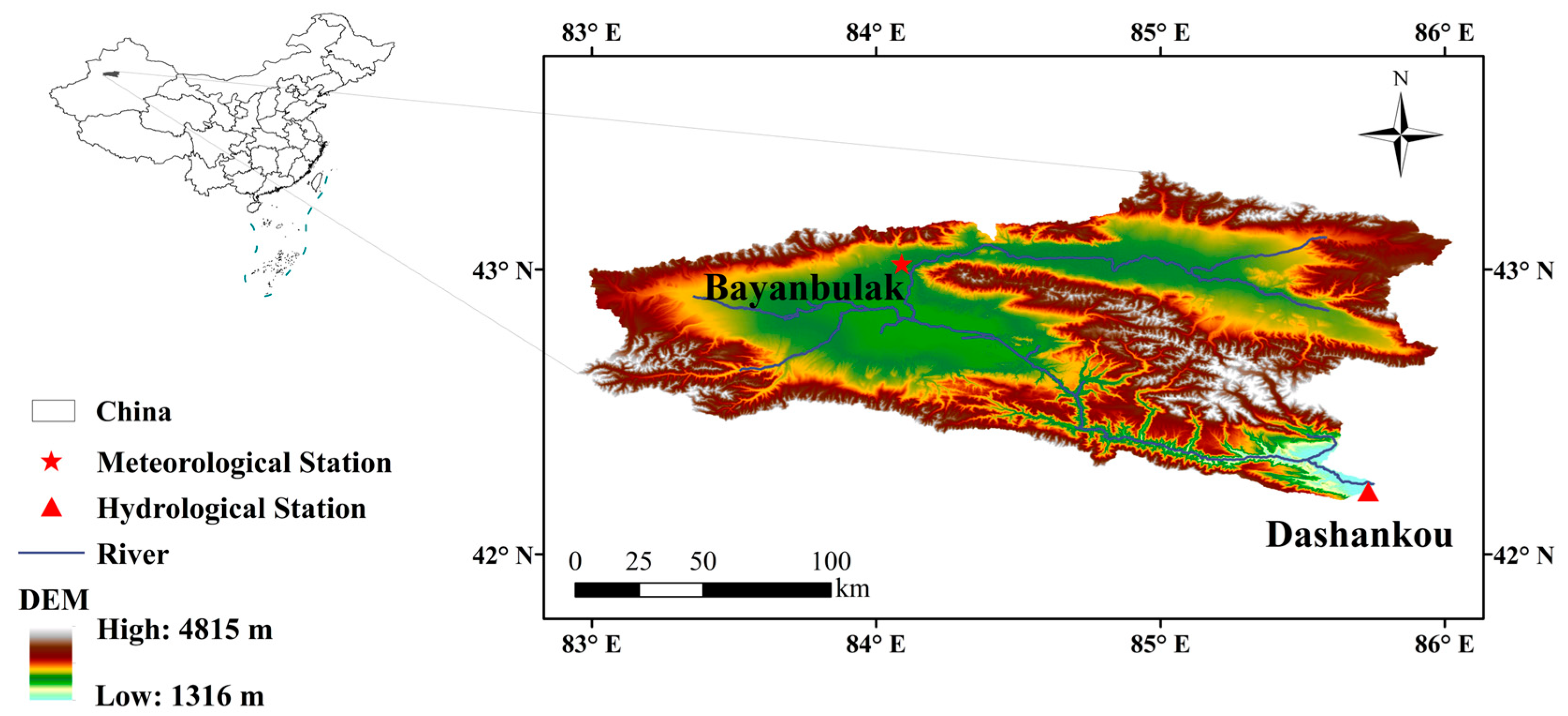
2.1. Study Area

Situated on the southern slope of Xinjiang’s Tianshan Mountains and the northern fringe of the Yanqi Basin, the Kaidu River Basin spans between 82°52′–86°55′ E and 41°47′–43°21′ N. It accounts for a large amount of the water production in the Bayingolin Mongol Autonomous Prefecture in Xinjiang. It is also the largest river flowing into the Yanqi Basin. The mountainous region of the basin boasts an average altitude of 3100 m, with a topography that descends from north to south, exhibiting a complex terrain. The catchment area above the mountain outlet approximates 1.9 × 10⁴ km2, and the river stretches 560 km from its source to the point where it feeds into the lake. It is the sole river that perennially replenishes Bosten Lake, China’s largest inland freshwater lake [25,26]. The Kaidu river is a mixed-type river, replenished by both snowmelt and precipitation. Seasonal snowmelt in spring and high mountain snowmelt coupled with mountain precipitation in summer primarily contribute to the river’s flow. Mixed rain and snow precipitation constitute 45.3% of the total runoff, while glacier meltwater accounts for 14.1%. The basin experiences an uneven distribution of annual precipitation, with noticeable seasonal influences. The maximum precipitation occurs from May to August. The distribution of evaporation throughout the year is uneven, with an annual evaporation of about 680 mm. The average annual runoff over multiple years is approximately 35.31 × 10⁸ m3, with 73.8% occurring during the flood season from April to September, and 26.2% during the dry season from October to March of the following year. A detailed overview of the basin is depicted in Figure 1.

2.2. Data

The research basin has only one meteorological station—the Bayanbulak Station. The Bayanbulak Station serves as the meteorological control station for the entire basin, with long-term series of observed data such as precipitation and temperature. Currently, many studies on the Kaidu River Basin also use data from this station to calculate and analyze the meteorological conditions and changes within the basin [27,28]. This study utilizes meteorological data from the Bayanbulak station in the Kaidu River Basin, encompassing daily temperature and precipitation measurements from 1975 to 2014, sourced from the China Meteorological Data website (http://data.cma.cn (accessed on 20 November 2018)). To analyze future meteorological changes, the Shared Socioeconomic Pathway (SSP) scenario (https://wcrp-cmip.org/model-intercomparison-projects-mips/scenariomip/ (accessed on 30 November 2023)) data under the IPCC’s sixth Coupled Model Intercomparison Project (CMIP6) were used in this study. The Shared Socioeconomic Pathways (SSPs), developed from the Representative Concentration Pathways (RCPs), quantitatively depict the interplay between climate change and socioeconomic trajectories, reflecting future societal challenges in climate change adaptation and mitigation [29,30]. These scenarios provide detailed projections of future population, economic growth, technological advancement, lifestyle, policy, and other social factors, outlining five socioeconomic development pathways: the sustainable development pathway (SSP1), the middle-of-the-road pathway (SSP2), the regional rivalry pathway (SSP3), the inequality pathway (SSP4), and the fossil-fueled development pathway (SSP5) [13,31,32,33]. We selected the CMIP6 model dataset released by eight global research institutions, which includes daily temperature and precipitation data for the Kaidu River Basin from 2025 to 2050 under four scenarios: SSP1-2.6, SSP2-4.5, SSP3-7.0, and SSP5-8.5. These data serve to analyze the basin’s future climate change patterns and trends (Table 1). The reference period is 1975–2014, and 2025–2050 is the future period.

3. Methods

3.1. Bias Correction Methods

Bias correction theory is based on the assumption that the statistical relationship between the data obtained from the current data sequence is still valid under future climate change scenarios, and uses statistical methods to reduce the bias between simulated values and observed values. The commonly used bias correction methods can be divided into two categories, one of which is based on statistical parameters such as mean and variance for correction, and the other is mainly based on probability distribution for correction [12]. In this study, seven methods that are both based on statistical parameter correction and probability distribution correction, such as linear scaling method (LS method) [34], DT method [35], EQM method [36,37], LOCI method [38], Gamma distribution mapping method [39,40], LOCI_QM combination method, and LOCI_Gamma combination method, are used to correct precipitation, and four methods such as linear scaling method (LS method), DT method, EQM method, and Normal distribution mapping method [41] are used to correct temperature. The specific introduction is as follows.

3.1.1. LS Method

The Linear Scaling method conducts a monthly-scale adjustment based on the discrepancy between the actual measured data and the original data, ensuring that the revised simulated monthly averages align with the actual measurements. Specifically, precipitation is adjusted using a factor derived from the ratio of the long-term monthly average of actual measurements to the simulated values. Meanwhile, temperature is corrected through the difference between the average actual observation data and the simulated values [42,43]. The detailed formula is presented below.
P r c o r , f u r , d = P r r a w , f u r , d × ( μ ( P r o b s , r e f , m ) / μ ( P r r a w , r e f , m ) )
T c o r , f u r , d = T r a w , f u r , d + μ ( T o b s , r e f , m ) μ ( T r a w , r e f , m )
In the formula, “Pr” and “T” represent precipitation and temperature, respectively, “raw” and “cor” represent the original output data of CMIP6 and bias-corrected data, respectively, “ref” and “fur” represent reference period and future period, respectively, “d” and “m” represent day and month, respectively, “μ” represents mean.

3.1.2. DT Method

The DT method is a technique that establishes the relationship between the actual measured daily precipitation or temperature (at different percentiles) and the raw simulated data through distribution mapping technology. This method corrects the errors in the raw simulated data by multiplying or adding the percentile ratio (for precipitation) or difference (for temperature) between the actual measured data and the raw simulated data to each percentile of the future time series [19,44,45]. The specific formula is as follows.
P r c o r , f u r , d = P r r a w , f u r , d × ( Q ( P r o b s , r e f , m ) / Q ( P r r a w , r e f , m ) )
T c o r , f u r , d = T r a w , f u r , d + Q ( T o b s , r e f , m ) Q ( T r a w , r e f , m )
In the formula, “Q” represents percentile, others are as Formulas (1) and (2).

3.1.3. EQM Method

The QM method is a non-parametric bias correction method, generally applicable to all possible distributions of precipitation or temperature, without the need for assumptions [46,47]. The QM method corrects meteorological data based on the daily empirical cumulative distribution functions (ECDFs) constructed at each point. In Empirical Quantile Mapping (EQM), the error correction of meteorological data is achieved by calculating the empirical cumulative distribution functions (ECDFs) based on the measured and simulated values, and taking the inverse function of the empirical cumulative distribution functions [36,37,48]. The specific formula is as follows.
P r c o r , f u r , d = e c d f o b s , r e f , m 1 ( e c d f r a w , r e f , m ( P r r a w , f u r , d ) )
T c o r , f u r , d = e c d f o b s , r e f , m 1 ( e c d f r a w , r e f , m ( T r a w , f u r , d ) )
In the formula, “ecdf” stands for empirical cumulative distribution functions. The rest is as Formulas (1) and (2).

3.1.4. DM Method

The Distribution Mapping (DM) method is a technique that assumes that the actual measured data and the model output values follow the same distribution. This method can be used to adjust the mean, standard deviation, and percentiles, and it retains extreme cases. For precipitation, the gamma distribution with shape parameters and scale parameters is commonly used and has been proven to be the most effective [39,46]. Due to the fact that the annual temperature in this research area shows a characteristic of being high in the middle and low at both ends, it conforms to the normal distribution based on the assumption of mean and standard deviation. Therefore, this study uses normal distribution to correct temperature [42,46]. The specific correction-transformation process is illustrated in Figure 2, exemplified by the Gamma partial mapping method. The specific formula is as follows.
P r c o r , f u r , d = F o b s , r e f , m 1 ( F r a w , r e f , m ( P r r a w , f u r , d ; α r a w , r e f , m , β r a w , r e f , m ) ; α o b s , r e f , m , β o b s , r e f , m )
T c o r , f u r , d = F o b s , r e f , m 1 ( F r a w , r e f , m ( T r a w , f u r , d ; μ r a w , r e f , m , σ r a w , r e f , m ) ; μ o b s , r e f , m , σ o b s , r e f , m )
In the formula “F” represents cumulative distribution functions. Assuming that precipitation follows Gamma distribution, “α” and “β” stand for shape parameter and scale parameter. Temperature follows Normal distribution and “μ” and “σ” stand for mean value and standard deviation. The rest is as Formulas (1) and (2).

3.1.5. LOCI Method

The LOCI method is a technique for correcting the frequency and intensity of wet days, aiming to effectively improve the excessive “drizzle” in the simulated raw data. This method usually includes two steps: (1) determining the wet-day threshold for each month based on the original precipitation series, to ensure that the frequency exceeding the threshold matches the measured wet-day frequency; (2) calculating the scale factor Sm based on the wet-day threshold, and applying it to the correction of future precipitation series [38,49,50]. The specific formula is as follows.
s m = μ ( P r o b s , r e f , d P r o b s , t h r e s ) P r o b s , t h r e s μ ( P r r a w , r e f , d P r r a w , t h r e s ) P r r a w , t h r e s
P r c o r , f u r , d = m a x [ ( P r o b s , t h r e s + ( P r r a w , f u r , d P r r a w , t h r e s ) ) × s m , 0 ]
In this formula “S” stands for scaling factor and “thres” stands for precipitation threshold, other terms are similar to Formulas (1) and (2).

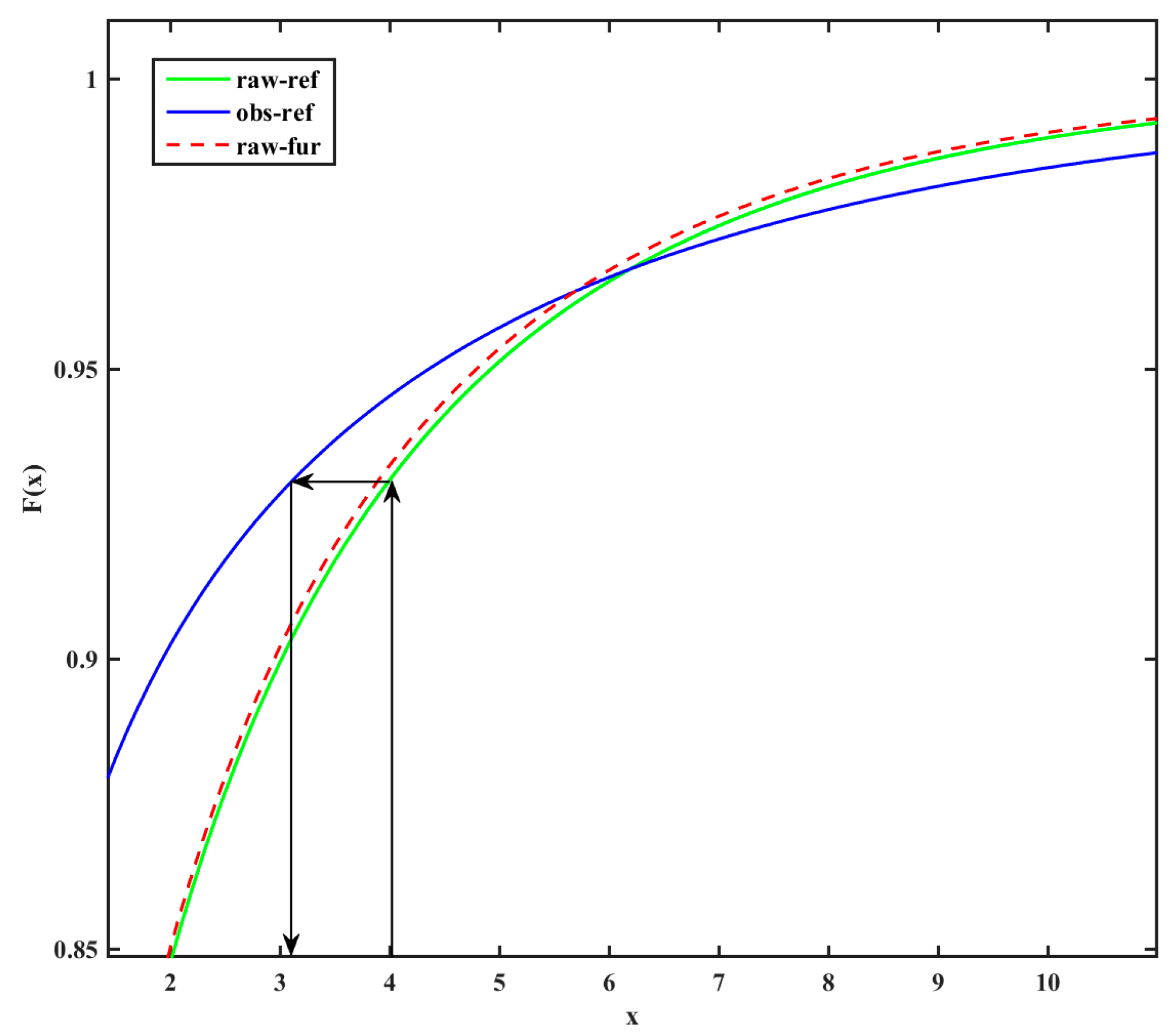
3.1.6. Combine Method

In this study, based on the individual application of the LOCI method, EQM method, and Gamma distribution mapping method for the correction of precipitation series, the combines of the LOCI method with the QM method and the combines of Gamma method were further developed, respectively. The LOCI_QM combination method and the LOCI_Gamma combination method are used, respectively, for the correction of the precipitation series. The specifics are as follows.
P r c o r , f u r , d = c d f o b s , r e f , m 1 ( c d f L O C I , r e f , m ( P r L O C I , f u r , d ) )
P r c o r , f u r , d = F o b s , r e f , m 1 ( F L O C I , r e f , m ( P r L O C I , f u r , d ; α L O C I , r e f , m , β L O C I , r e f , m ) ; α o b s , r e f , m , β o b s , r e f , m )
In the formula “F” denotes cumulative distribution functions, “LOCI” represent data corrected by the LOCI method. “ c d f o b s , r e f , m ” is calculated from observed data during reference period, “ c d f L O C I , r e f , m ” represents the cumulative distribution function calculated from data corrected by the LOCI method during the reference period. The rest is as Formulas (1) and (2).

3.1.7. Evaluation Indicators

This study selects indicators based on frequency and time series to evaluate the performance of bias correction methods. The frequency indicators mainly include mean, standard deviation, median, percentiles, frequency of wet days (precipitation), intensity of wet days (precipitation), etc. The time-series indicators mainly include Mean Absolute Error (MAE) and Root Mean Squared Error (RMSE), etc. Among them, the smaller the values of MAE and RMSE, the closer the bias-corrected values are to the measured values. The specific formula is as follows.
M A E = i = 1 n | Y i o b s Y i c o r | n
R M S E = i = 1 n ( Y i c o r Y i o b s ) 2 n
Y i o b s and Y i c o r refer to the ith elements of the data series.

3.2. Extreme Climate Indicators

In order to better understand and analyze the future trend of meteorological conditions in the Kaidu River Basin, in this study, based on the analysis of precipitation and temperature trends, the extreme climate indicators were selected to study future extreme climate events in the Kaidu River Basin. For precipitation, in order to explore the trend of extreme precipitation intensity and frequency in the future, we selected indicators such as R95p and CDD for analysis, where the total precipitation amount for days exceeding the 95% percentile of daily rainfall is denoted as R95p, while CDD represents the maximum number of consecutive days with precipitation less than 1 mm [51,52,53,54]. For temperature, based on daily average temperature data, the maximum daily average temperatures of each month were selected for the analysis.

4. Results

4.1. Analysis of Bias Correction Methods

For precipitation, this paper evaluates the correction effects of various methods based on frequency evaluation indicators such as mean, standard deviation, median, percentiles, wet-day frequency and intensity, and time-series evaluation indicators such as RMSE and MAE. Table 2 presents the evaluation metrics following the correction of output data by seven different precipitation bias correction methods from various institutions, as well as the average results after computing the mean of the metrics from eight institutions. Specifically, Nos. 1–9 display the results of the evaluation metrics after bias correction for each institution’s data, while No. 10 shows the result after averaging the evaluation metrics from all eight institutions. The purpose is to eliminate the influence of individual institutional data to more clearly assess the corrective effectiveness of the bias correction methods. As can be seen from Table 2, all seven correction methods have a certain corrective effect on the frequency and time-series indicators of raw data outputs, and after corrections by various methods, each metric has become more closely aligned with the observed values. Compared with raw data, the LS method has the best correction effect on the mean with a relative deviation of 0. However, the LS method has unsatisfactory correction effects on other indicators and has a larger error compared to the measured data. The DT method has obvious correction effects on the median, 90% percentile and 75% percentile with their relative deviations being, respectively, 0%, 1.5%, and −5%. The EQM method and LOCI_QM method have effects on the standard deviation and 95% percentile with their relative deviations both being 0 and −1.36%. Additionally, a comparison between the two methods reveals that combining LOCI with QM yields correction results that are essentially similar to those of the EQM method. Meanwhile, the Gamma distribution mapping method and LOCI_Gamma method have optimal corrections for wet-day intensity and frequency with their respective relative deviations being approximately 4.29% and 0.4%. Moreover, when examining the results of wet-day frequency correction, the LOCI_Gamma method outperforms the Gamma method. It can be seen that different methods have different focuses in correcting frequency indicators based on their principles.
In terms of evaluation metrics for time series, compared to the raw data series, all seven bias correction methods show improvements, with the RMSE and MAE values of the seven methods not differing significantly. The results corrected by the LOCI method, when compared with actual measured data, yield the smallest RMSE and MAE. This indicates that the LOCI method outperforms the other six methods in time-series correction. Based upon bias correction methodology assessment results, LOCI_Gamma is selected to correct the precipitation data for subsequent analysis.
Regarding temperature, the four correction methods employed in this study all demonstrated effective correction results. The frequency indicators included mean, standard deviation, median, and percentiles, while the time-series indicators comprised MAE and RMSE. Subsequently, these indicators were used to evaluate the calibration effectiveness of various bias correction methods. Table 3 displays the evaluation metrics results for four temperature bias correction methods applied to the output data from various institutions, as well as the average results after calculating the mean of the metrics from eight institutions. Specifically, Nos. 1–9 show the individual results of the evaluation metrics after error adjustment for each institution’s data, while No. 10 presents the result after averaging the evaluation metrics across all eight institutions.
As can be seen from Table 3, the four correction methods used all have a certain correction effect on the frequency and time-series indicators on the raw data. The four methods exhibit minimal differences in their bias correction effectiveness, and compared to the original data, the improvements in frequency indicators by each bias correction method are modest. However, the frequency indicators of the corrected data are relatively close to the observed data, and the temperature series overall demonstrates a good simulation effect. Among them, the DT method has the best correction effects on frequency indicators such as the mean, standard deviation, median, 95%, 90%, and 75% percentiles, with their relative deviations being 0, 0, −10%, −0.49%, −0.18%, and −0.62%, respectively. At the same time, the Normal distribution mapping method exhibits mediocre performance in terms of the median, with certain errors compared to the observed data, while it performs well in other aspects. The LS method shows good results for the mean and standard deviation, but is mediocre for the median and percentiles, presenting a larger discrepancy in correction effectiveness when compared to the other three methods. For the evaluation indicators of the time series, the LS method has an RMSE value of 6.27, which is the lowest among the four methods, indicating the most optimal correction effect in terms of RMSE. Both the EQM and Normal distribution mapping methods have the lowest MAE value at 4.67 among the four methods, and their RMSE values are 6.3, differing by only 0.03 from the LS method. Overall, the EQM and Normal distribution mapping methods perform well in terms of time-series indicators. Based on the evaluation results of the bias correction method, considering that the EQM method has certain limitations for extreme value correction, the Normal distribution mapping method is selected in this study to correct the temperature data for subsequent analysis.
Next, this study calculated the correlation coefficients between the corrected monthly precipitation, temperature data and the measured data. Table 4 and Table 5, respectively, display the monthly scale correlation coefficients between the original output data and the meteorological data corrected by seven methods, compared with the observed meteorological data, using the averaged results from eight institutions. As indicated in Table 4, the monthly scale correlation coefficient between the original precipitation data and the observed precipitation data is 0.33. It is evident that due to the variation in precipitation sequences and the uncertainty of climate model predictions, the original output of precipitation data from GCMs is generally quite coarse, differing significantly from measured values, and cannot be used directly. After bias correction, all correlation coefficients have improved to above 0.7, showing a marked enhancement, which further indicates an increase in the reliability of data after bias correction. In addition, although there is not much difference in correlation coefficients between various bias correction methods, compared to using the Gamma distribution mapping method or LOCI method alone, the combined LOCI_Gamma method has slightly improved correlation coefficients with the measured data. Meanwhile, as shown in Table 5, the monthly correlation coefficient between the original temperature data and the measured temperature data is 0.94. It can be seen that the simulation effect of the temperature data output by GCMs is better. Compared with the raw data, the correlation coefficient of the corrected data has been improved, both of which are 0.97.

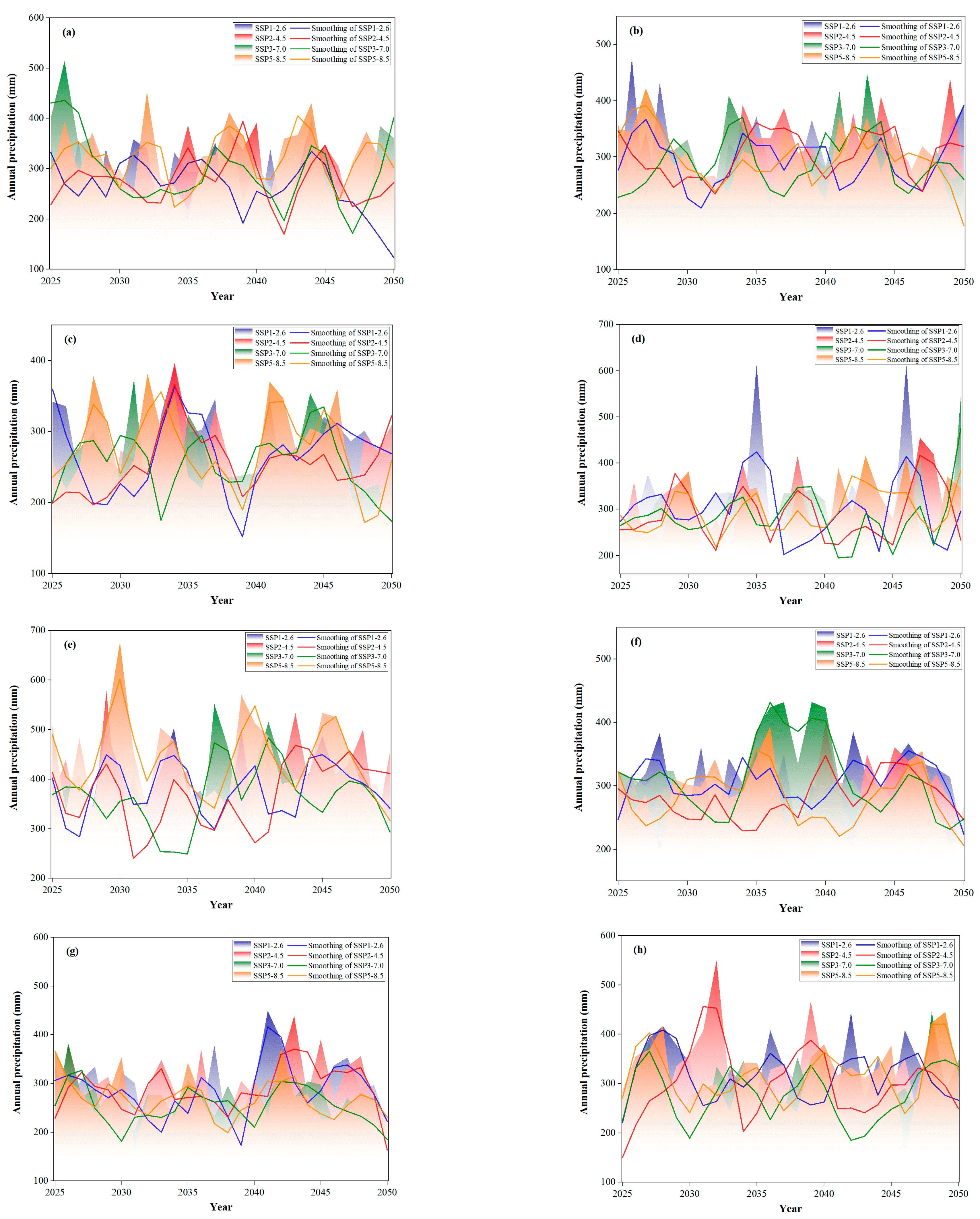
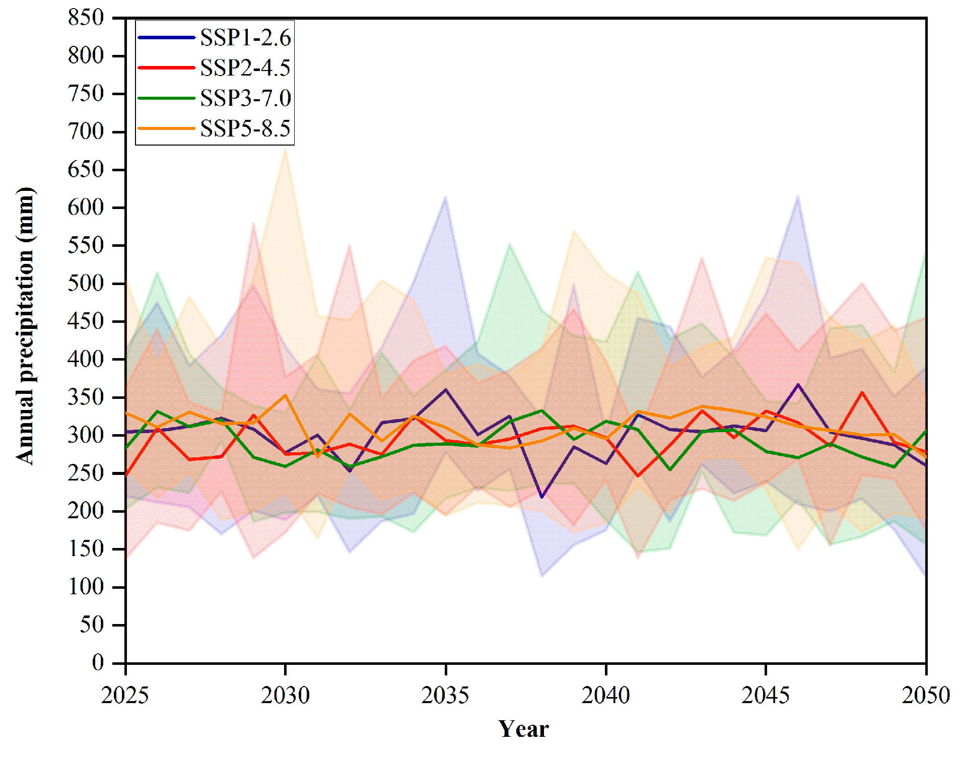
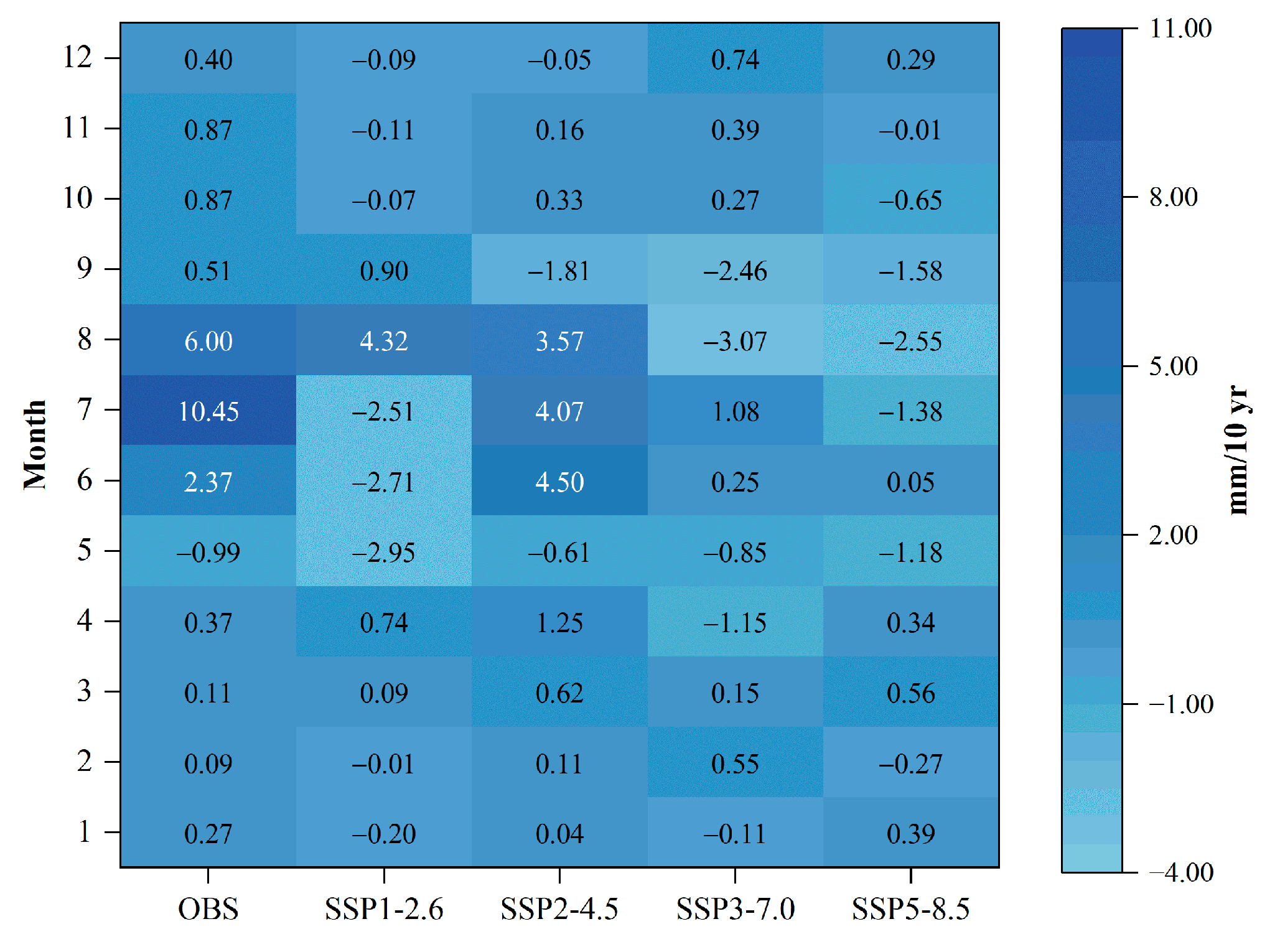
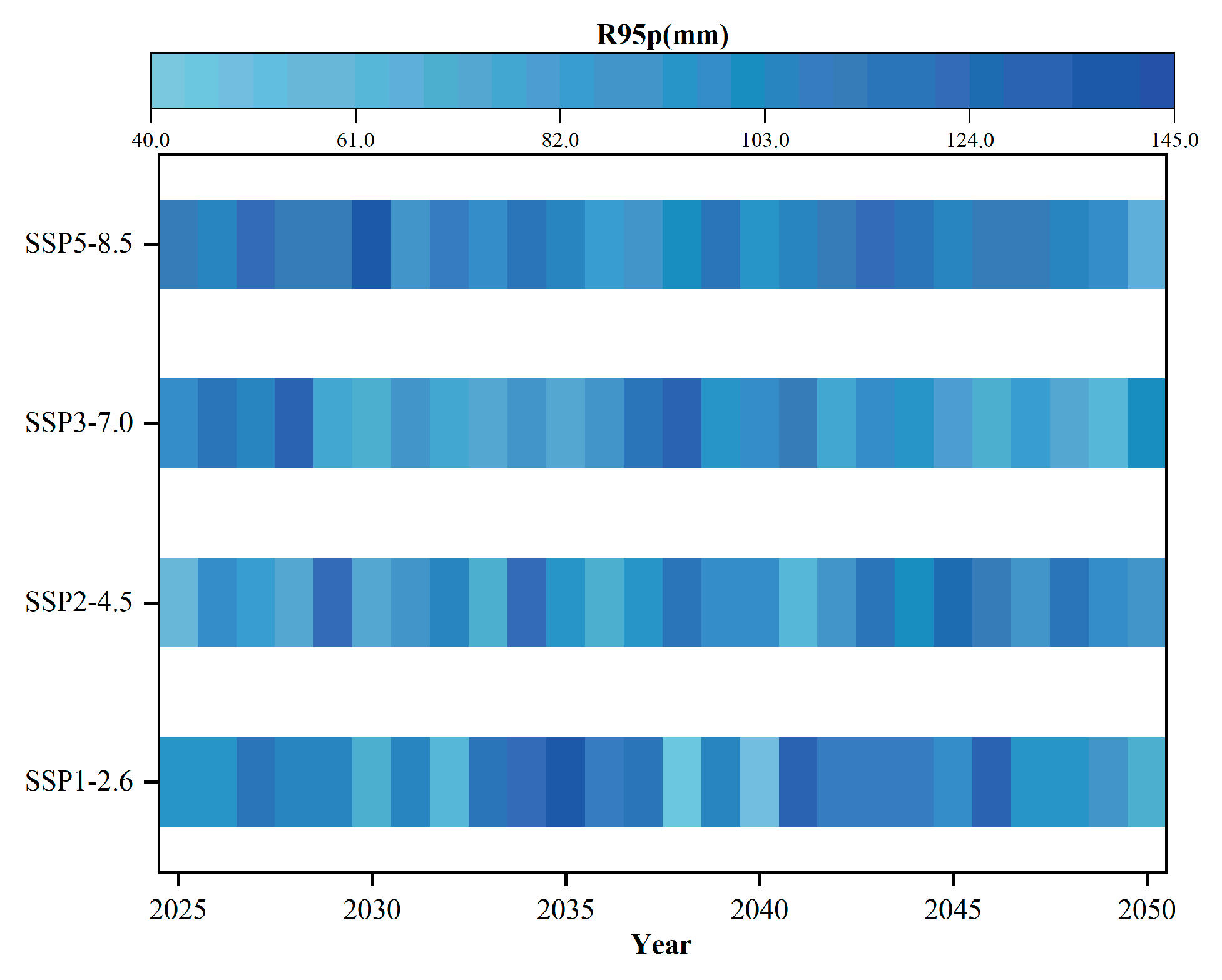
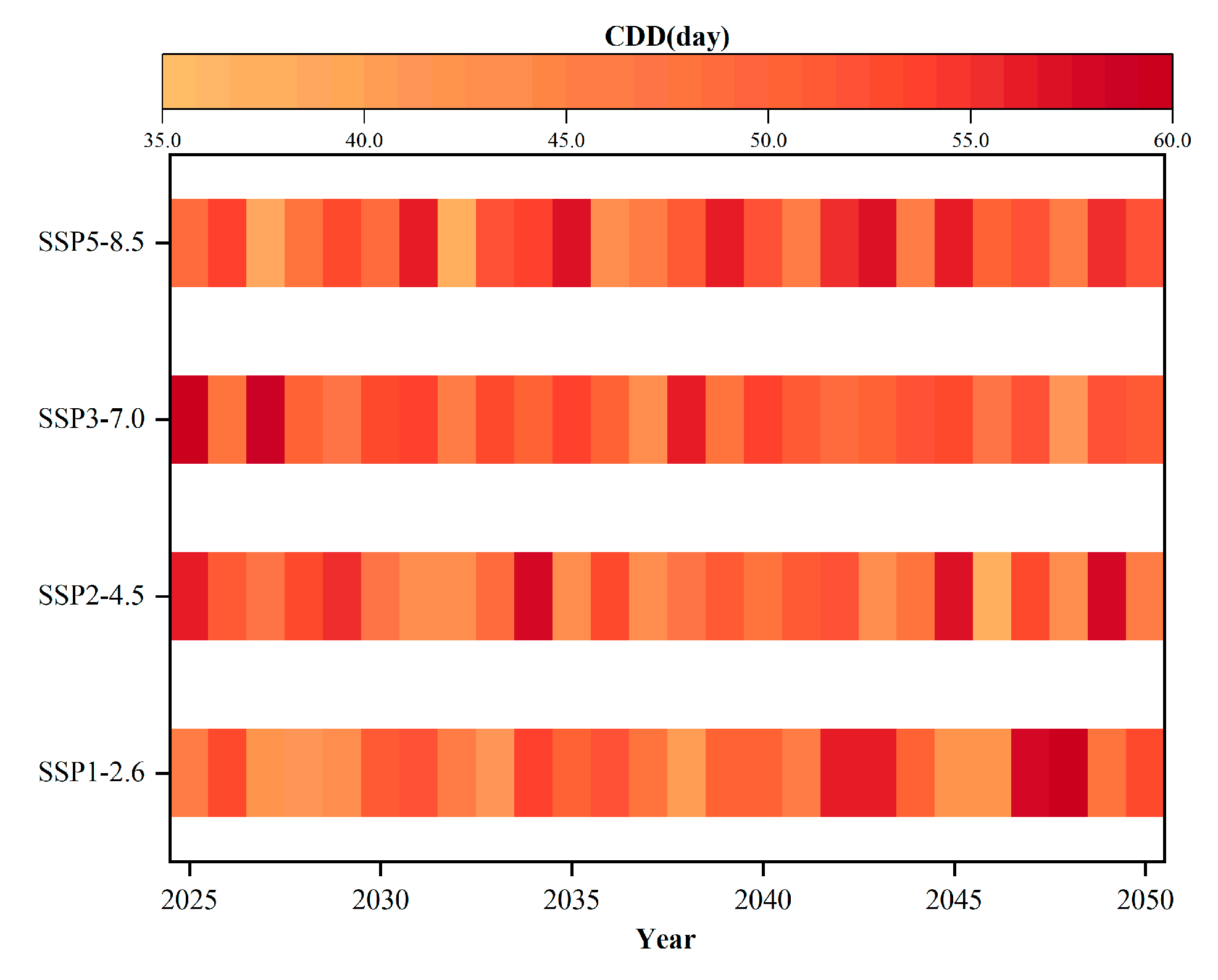
4.2. Precipitation Trend and Extreme Value Analysis

Next, this study employed linear regression analysis to examine the changes in annual precipitation totals in the Kaidu River Basin during the historical period (1975–2014) and the future period (2025–2050). It can be seen that the annual precipitation in the research basin during the historical period shows a basically upward trend, with a change rate of 21.32 mm/10 yr and an average annual precipitation of 272.94 mm. According to the evaluation results of the bias correction method, the LOCI_Gamma correction result (Figure 3 and Figure 4) is selected for analysis (the same as below). In Figure 3, the changes in annual precipitation for future periods, as corrected for bias in the output data from eight institutions, are displayed. Four color bands represent the variations in precipitation under four scenarios: SSP1-2.6, SSP2-4.5, SSP3-7.0, and SSP5-8.5. The peaks of the color bands correspond to the annual precipitation for each year, while the line graph represents the smoothed trends of annual precipitation changes. Figure 4 illustrates the changes in annual precipitation averaged across eight institutions, with four color bands representing the range of precipitation changes under four scenarios: SSP1-2.6, SSP2-4.5, SSP3-7.0, and SSP5-8.5. The low peaks within the color bands indicate the minimum annual precipitation values among the eight institutions, while the high peaks represent the maximum values. The line graph depicts the trend of the averaged annual precipitation changes. It can be seen that the total annual precipitation under the SSP1-2.6, SSP3-7.0, and SSP5-8.5 scenarios in the future period shows a downward trend, with change rates of −2.59 mm/10 yr, −4.22 mm/10 yr, and −5.98 mm/10 yr, respectively. The total annual precipitation under the SSP2-4.5 scenario shows an upward trend, with a change rate of 12.17 mm/10yr. The average annual precipitation under the four scenarios of SSP1-2.6, SSP2-4.5, SSP3-7.0, and SSP5-8.5 is 301.95 mm, 295.57 mm, 291.05 mm, and 311.52 mm, respectively. By analyzing the precipitation change trend, it can be seen that, in the future period, precipitation is projected to exhibit an increasing trend under the SSP2-4.5 scenario. Conversely, a declining trend in multi-year average precipitation is anticipated across the remaining three scenarios. Specifically, in terms of precipitation, compared with the historical period, the average annual precipitation in the future period is higher than that in the historical period under the SSP1-2.6, SSP2-4.5, SSP3-7.0, and SSP5-8.5 scenarios, and the average annual precipitation values under the four scenarios are 10.63%, 8.29%, 6.64%, and 14.13% higher than those in the historical period, respectively. Further, the monthly precipitation change trends in the historical and future periods are shown in Figure 5 and Figure 6. Compared with the historical period, the monthly precipitation from January to December basically increases, but the monthly precipitation increase rate has a clear decreasing trend in total in the future period. In addition, it can be seen that, in July, the precipitation increase rate has decreased from 10.45 mm/10 yr in the historical period to −2.51 mm/10 yr (SSP1-2.6), 4.07 mm/10 yr (SSP2-4.5), 1.08 mm/10 yr (SSP3-7.0), and −1.38 mm/10 yr (SSP5-8.5).
Further, this paper calculates the extreme precipitation indicator R95p for both historical and future periods based on the analysis of total amount of annual precipitation and their trends, thereby reflecting the situation of extreme precipitation within the basin. The calculation results (Figure 7) show that the R95p in the historical period is on an upward trend, with a maximum value of 219.2 mm in 1999 and a minimum value of 9.8 mm in 1979. In the future period (2025–2050), the R95p shows a downward trend under the SSP1-2.6, SSP3-7.0, and SSP5-8.5 scenarios, while it shows an upward trend under the SSP2-4.5 scenario, consistent with the trend of annual precipitation. The maximum values of R95p under the four scenarios of SSP1-2.6, SSP2-4.5, SSP3-7.0, and SSP5-8.5 in the future period are 139.09 mm (2035), 126.71 mm (2045), 130.57 mm (2038), and 140.94 mm (2030), respectively, and the minimum values are 44.67 mm (2038), 59.58 mm (2025), 62.90 mm (2049), and 64.66 mm (2050), respectively. Compared with the historical period, the R95p values in the future period under the four scenarios are generally distributed between 80–130 mm. By comparing the averages, it can be seen that the average R95p values under the SSP1-2.6, SSP2-4.5, and SSP5-8.5 scenarios in the future period are higher than those in the historical period, and they show an increase trend under the SSP5-8.5 scenario, with extreme precipitation values generally higher than 100 mm, an increase of 15.04% compared to the historical period. In terms of temporal distribution, extreme precipitation in the historical period mainly occurs from June to August, while in the future period, the months with extreme precipitation increase markedly, basically concentrated from May to September, and the time range expands more obviously with the increase in radiative forcing.
In addition, this paper calculates the extreme precipitation index CDD to reflect the number of consecutive dry days within the basin. Figure 8 shows the CDD under different scenarios in the future period. According to the calculation, the CDD in the historical period is on a downward trend, with a maximum value of 107 days in 1989 and a minimum value of 30 days in 2010. In the future period, the CDD shows an upward trend under the SSP1-2.6 and SSP5-8.5 scenarios, while it shows a downward trend under the SSP2-4.5 and SSP3-7.0 scenarios. By comparison, it can be seen that the changes in CDD under the four scenarios are relatively small, with the number of dry days basically around 50 days, and compared to the historical period CDD (68 days), the CDD in the future period under the four scenarios has decreased, indicating a reduction in the number of consecutive dry days in the future.

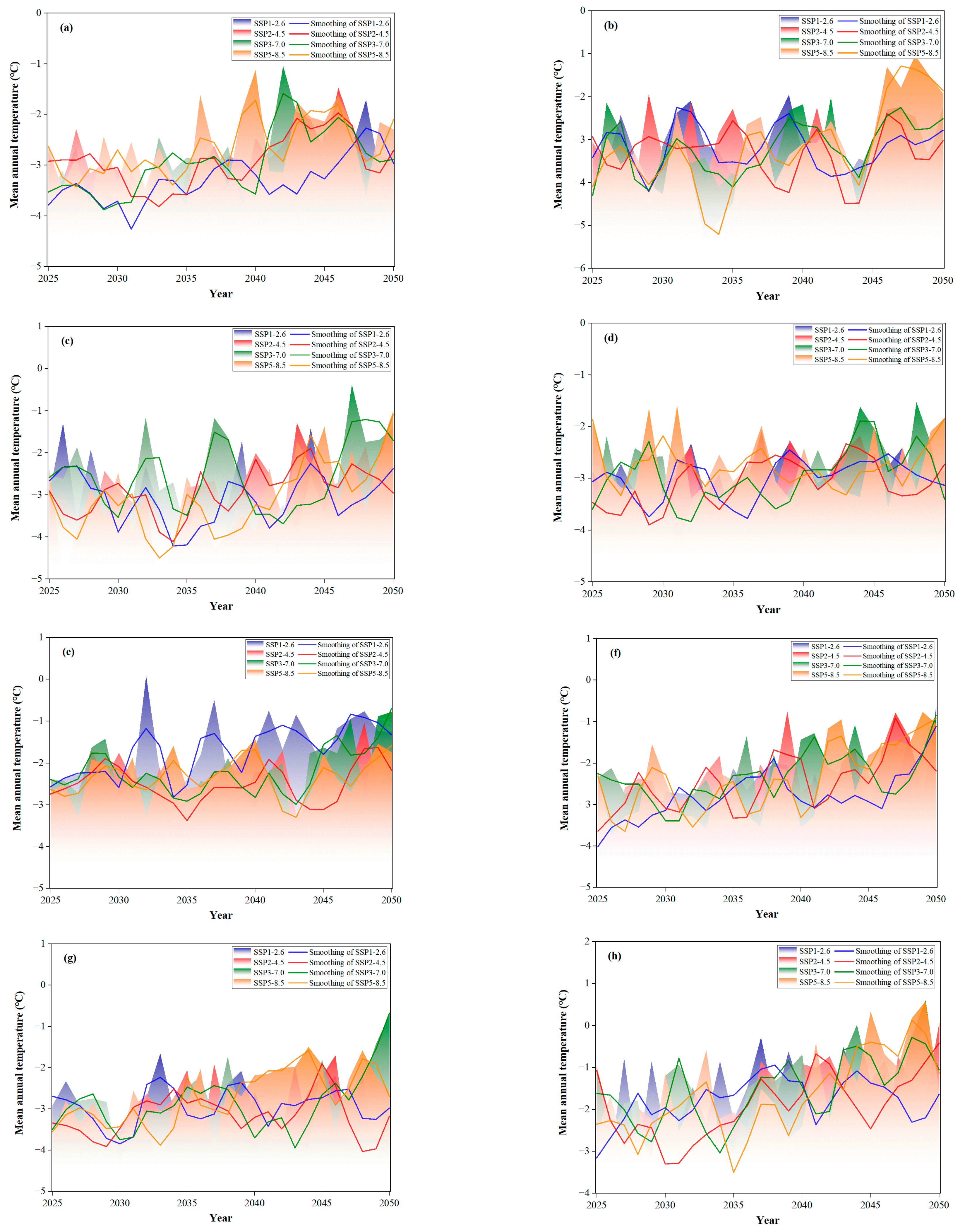
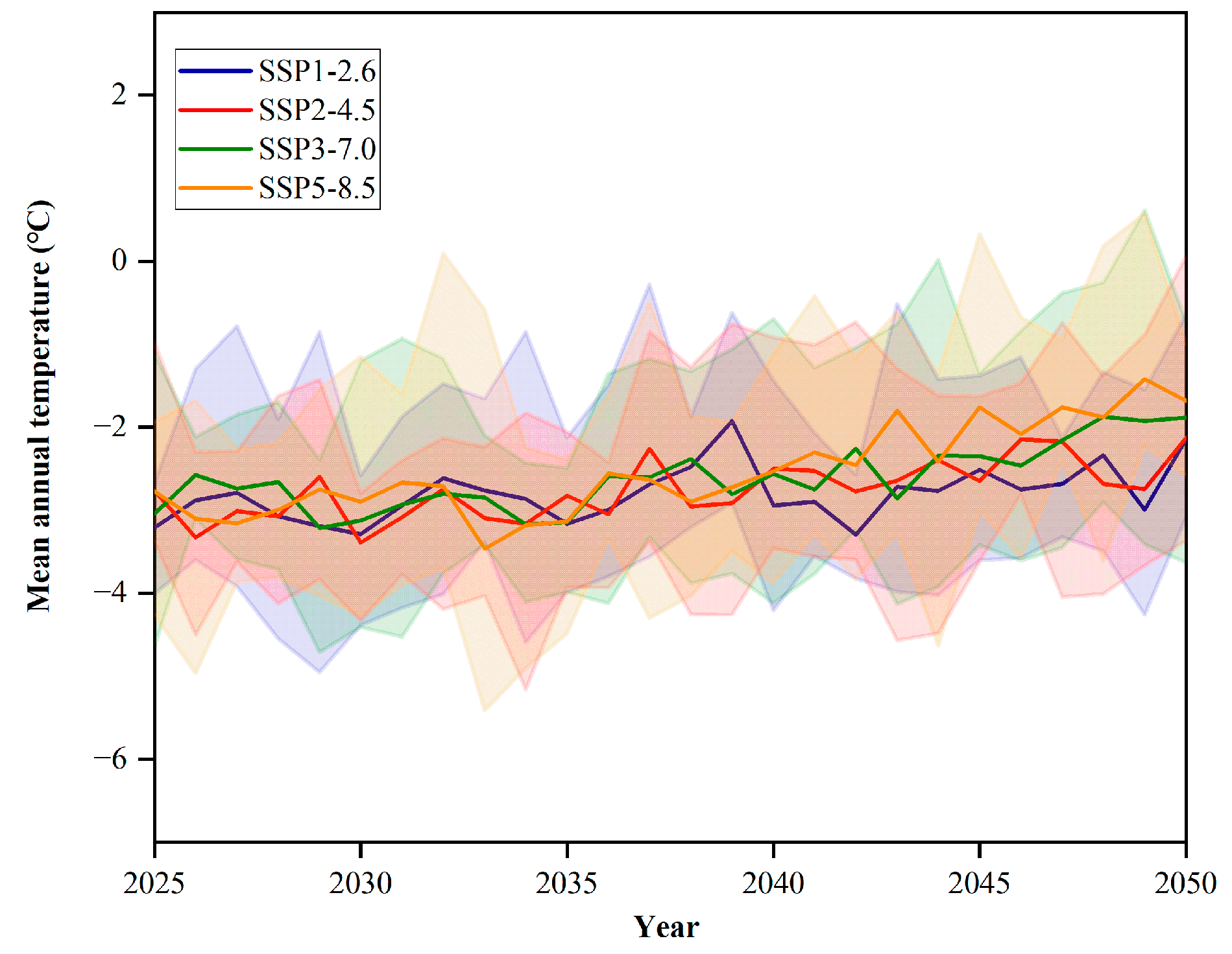
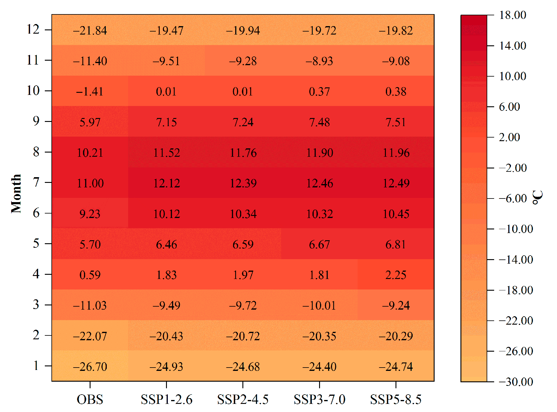
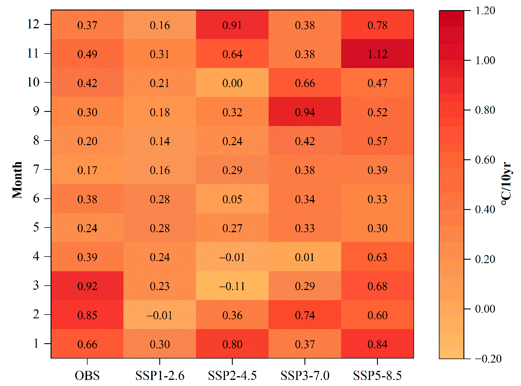
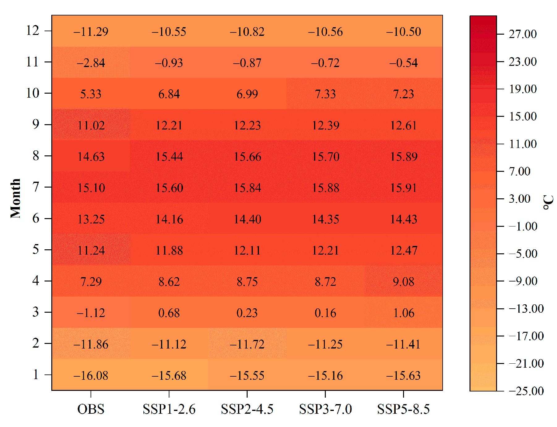
4.3. Temperature Trend and Extreme Value Analysis

Similarly, this study utilized linear regression analysis to examine the annual average temperature changes during the historical period (1975–2014) and the future period (2025–2050). It is evident that the annual average temperature during the historical period shows a obvious upward trend, with a rate of change of 0.45 °C/10 yr and a multi-year average temperature of −4.24 °C. Based on the results of the bias correction method evaluation, the Normal distribution mapping method correction results (Figure 9 and Figure 10) are selected for analysis. In Figure 9, the changes in the annual average temperature for future periods, as corrected by the output data from eight institutions, are depicted. Four color bands represent the variations in temperature under four scenarios: SSP1-2.6, SSP2-4.5, SSP3-7.0, and SSP5-8.5. The peaks of the color bands correspond to the annual average temperature values for each year, while the line graph represents the smoothed trends of annual average temperature changes. Figure 10 illustrates the changes in the annual average temperature after averaging the data from eight institutions. Four color bands represent the temperature variation ranges under four scenarios: SSP1-2.6, SSP2-4.5, SSP3-7.0, and SSP5-8.5. The low peaks within the bands indicate the minimum annual average temperatures recorded by the institutions, while the high peaks represent the maximum values. The line graph depicts the trend of change in the averaged annual average temperatures. It can be seen that under the SSP1-2.6, SSP2-4.5, SSP3-7.0, and SSP5-8.5 scenarios, the annual average temperatures in the future period all show an upward trend, with rates of change of 0.21 °C/10 yr, 0.31 °C/10 yr, 0.39 °C/10 yr, and 0.60 °C/10 yr, respectively. The multi-year average temperatures under the four scenarios of SSP1-2.6, SSP2-4.5, SSP3-7.0, and SSP5-8.5 are −2.80 °C, −2.76 °C, −2.62 °C, and −2.53 °C, respectively. Comparative analysis shows that, compared with the historical period, the annual average temperature in the future period under the four scenarios is higher than that in the historical period, and the higher the radiative forcing, the more obvious the warming. It can be calculated that the multi-year average temperature values under the four scenarios are 33.96%, 34.91%, 38.21%, and 40.33% higher than those in the historical period, respectively. Furthermore, by analyzing the trends of monthly average temperature changes in the historical and future periods, it can be seen from Figure 11 that during the historical period and future periods under four different SSP scenarios, the monthly average temperatures from January to December show different changes. In addition, the OBS column represents the multi-year average of monthly average temperatures for the historical period (1975–2014), while columns SSP1-2.6 to SSP5-8.5 represent the multi-year averages of monthly average temperatures for eight institutions in future periods (2025–2050). Overall, Figure 11 and Figure 12 illustrate that the monthly average temperatures in all months from January to December in the future period under the four scenarios have increased. The monthly average temperature increase rates under different scenarios show irregular trends, but in the SSP5-8.5 scenario, except for February, March, and June, the temperature increase rates in the remaining months have increased markedly. In August and November, the rates have increased from 0.20 °C/10 yr and 0.49 °C/10 yr to 0.57 °C/10 yr and 1.12 °C/10 yr, respectively, with increases of 185% and 129%, respectively.
Building on the analysis of the trends in annual average temperature changes, this study further calculated the maximum daily average temperatures for both the historical and future periods. Specifically, the maximum daily average temperatures for each month were calculated and then averaged over multiple years, with the detailed results presented in Figure 13. The figure indicates that, compared to the historical period, the maximum daily average temperatures for each month have increased under all four future scenarios, with the SSP5-8.5 scenario showing a particularly notable rise in temperatures. Additionally, the most significant increase in the maximum daily average temperature is observed in March, with the increments under the four scenarios SSP1-2.6, SSP2-4.5, SSP3-7.0, and SSP5-8.5 being 160.71%, 120.54%, 114.29%, 194.64%, respectively. This indicates that not only is there a rising trend in the annual average temperature for future periods, but also a notably pronounced increase in the maximum daily average temperatures.

5. Discussion

5.1. The Applicability of Bias Correction Methods for CMIP6 in the Arid Area of Northwest China

The Kaidu River Basin is located in the arid region of northwest China. Within the research area, there are few on-site meteorological and hydrological stations, making data acquisition difficult, which is one of the challenges in studying this region. There is only one meteorological station in the Kaidu River Basin—Bayanbulak Station, which is situated upstream of the basin and serves as a controlling meteorological site for the entire basin with long-term recorded precipitation and temperature data. Therefore, this study uses historical precipitation and temperature measurements from Bayanbulak Station to correct CMIP6 original data using different bias correction methods, aiming to investigate and compare the applicability of these methods within the research basin. The analysis in this manuscript finds that overall, this meteorological station has a certain representativeness and applicability for the overall meteorological conditions of the basin; hence, in the absence of additional data supplementation, it can be used to represent conditions across the basin.
This study found that by analyzing the correlation coefficients between CMIP6 raw data and measured data, the GCM temperature simulation results are relatively close to actual conditions, while precipitation simulation results differ significantly from reality, which is consistent with other related studies [55,56]. For precipitation, all eight institutions overestimated precipitation to some extent and also overestimated wet-day frequency. Based on bias correction results and evaluation indicators, further analysis shows that using bias correction methods has a more apparent effect on correcting precipitation; for temperature data, there is also some improvement after correction but it is not very significant since the original data themselves are not far off from actual observations. At the same time, due to the different principles behind various bias correction methods, their effects on different evaluation indicators also vary. For example, for precipitation, the LS method based on mean values provides optimal mean value correction for model output precipitation sequences but only corrects raw data based on mean comparisons. Therefore, compared with other methods, the LS method’s performance in correcting other frequency indicators such as standard deviation, median value, wet-day frequency and intensity is poorer. The DT method based on quantile mapping principles along with the EQM and LOCI_QM combined methods provide optimal corrections for percentiles of model output precipitation sequences as well as median values and standard deviations. Further comparison between the EQM method and LOCI_QM method reveals that both yield essentially identical results in terms of corrections made and evaluation indicator outcomes; combining them does not modify the distribution of original rainfall; when applied together their corrective effect shows no difference from EQM alone without any definite improvement noted. The Gamma distribution mapping method combined with LOCI_Gamma optimally corrects wet-day intensity and frequency. Compared to the Gamma method alone, LOCI_Gamma further improves corrections made to wet-day frequency and intensity while simultaneously modifying the distribution of original rainfall somewhat during its adjustments for wet-day frequency/intensity metrics; however, when applying Gamma distribution it assumes future periods share identical distribution functions with historical periods which does not fully align with reality, hence this approach still has certain flaws in this respect. In the context of extreme value correction, the EQM method tends to underestimate the range of extreme values due to its inherent characteristics, which may result in significantly underestimated maximums or overestimated minimums in the corrected data. Therefore, when dealing with extreme values in meteorological data, the applicability of the EQM method for extreme value processing should be carefully considered. Consequently, for different bias correction objectives, an appropriate error correction method should be selected based on a comprehensive consideration of watershed characteristics and target requirements.

5.2. Future Changes of Extreme Climatic Events in River Basins

By analyzing the historical and future changes of meteorological data such as precipitation and temperature in the basin, it can be seen that the annual average precipitation and temperature in the future period are higher than those in the historical period. Based on further analysis, it can be seen that under the moderate development scenario (SSP2-4.5), the annual precipitation in the study area shows an upward trend. Under the sustainable development scenario (SSP1-2.6), regional competition development scenario (SSP3-7.0), and traditional fossil fuel-dominated development scenario (SSP5-8.5), despite the total precipitation still being higher than the historical period, over the next 26 years, there is an overall downward trend in annual precipitation. So, more attention should be paid to the availability of future water resource in the basin.
Regarding extreme precipitation events, historically, they mainly occurred between June and August. However, in the future, the months during which extreme precipitation events occur are expected to increase significantly, primarily concentrating between May and September. Additionally, as radiative forcing intensifies, the temporal range of extreme precipitation events is also likely to expand. Therefore, it is necessary to plan and arrange water resources in advance for future extreme precipitation events. At the same time, the number of dry days in the future period (50 days) is reduced compared to the historical period (68 days). We speculate that this may be due to an increase in total precipitation in the future compared to the historical period, as well as a longer distribution of precipitation events, which consequently reduces the number of consecutive dry days in the future.
Further analysis of future precipitation extremes reveals that under the SSP1-2.6 and SSP5-8.5 scenarios, as temperatures continue to rise, a declining trend in basin precipitation is expected, with an increasing occurrence of high temperatures and scarce rainfall within the basin. This may lead to a higher probability of meteorological drought events. Such conditions are likely to result in a shortage of water resources in the future and affect the basin’s self-regulation capacity. On the other hand, considering the Kaidu River’s role in providing ecological water supply to Bosten Lake, it is essential to plan and manage the river basin’s water resources rationally to mitigate the decline in water levels of Bosten Lake and maintain its normal ecological functions. In summary, it is evident that future development scenarios will significantly impact the water resource changes within the Kaidu River Basin, and maintaining a stable and sustainable development within the basin is crucial for preserving its self-regulation capabilities and ensuring the supply of water to downstream Bosten Lake.

6. Conclusions

This study selected precipitation and temperature data for the future period (2025–2050) under four different SSP scenarios from eight institutions in CMIP6. These data were compared with the observed precipitation and temperature data for the historical period (1975–2014) in the Kaidu River Basin. Various bias correction methods were applied to correct the raw precipitation and temperature data output by the GCMs. The applicability of different bias correction methods was analyzed, and the evolution patterns of important meteorological elements and extreme values in the basin during the future period were further interpreted. The conclusions are as follows:
(1) Based on the correction results and evaluation indicators of precipitation and temperature, it is known that due to the different principles of various bias correction methods, their effects during the correction process also vary. The bias correction method adopted in this paper has a certain corrective effect on both precipitation and temperature. Compared to temperature, the corrective effect of each method on precipitation is more obvious. For temperature, although there is not much difference in the effects of different bias correction methods, there is a slight improvement in the accuracy of overall temperature data after correction. The LS method shows better results in terms of mean values but performs poorly on other evaluation indicators; its corrective effect is somewhat lacking. When using the EQM method for corrections, special attention should be paid to its effectiveness in correcting extreme values. Meanwhile, for precipitation, by comparing and analyzing combined methods with original methods based on evaluation indicator results, it can be seen that compared to single methods, the LOCI_QM method does not show much difference in corrective effect from single methods. However, the LOCI_Gamma method can further modify precipitation based on single methods and therefore exhibits better overall corrective performance.
(2) In the future period, the annual precipitation and average temperature in the Kaidu River Basin are higher than in the historical period. The average annual temperature shows an upward trend in the future period, but the overall trend of annual precipitation decreases in the future period, except for the SSP2-4.5 scenario. Compared with the historical period, the frequency of extreme precipitation events under the SSP1-2.6, SSP2-4.5, and SSP5-8.5 scenarios in the future period is higher than in the historical period, and the number of rainless days has decreased. In the future, under the SSP1-2.6 and SSP5-8.5 scenarios, the probability of high-temperature drought events in the basin may further increase, while, under the SSP2-4.5 scenario, the situation of high temperature and heavy rainfall in the basin may become more prominent. This reminds us that we need to pay more attention to the effective regulation and management of water resources in river basins and regions.

Author Contributions

Conceptualization, C.C., Y.W. and L.F.; methodology, C.C.; validation, C.C. and Y.W.; formal analysis, C.C. and Y.W.; investigation, C.C.; resources, Y.W.; data curation, C.C. and J.D.; writing—original draft preparation, C.C. and Y.W.; writing—review and editing, C.C., Y.W. and L.F.; project administration, W.C. and Y.W. All authors have read and agreed to the published version of the manuscript.

Funding

This research was funded by the Strategic Priority Research Program of the Chinese Academy of Sciences, grant number XDA23020102; Jiangsu Natural Resources Development Special Fund for Marine Science and Technology Innovation, grant number JSZRHYKJ202205; the Jiangsu Province Natural resources Science and Technology Project, grant number 2022016; the Guangdong Foundation for Program of Science and Technology Research, grant numbers 2019B121201004, 2019QN01L682; the National Natural Science Foundation of China, grant number 42177065; National Key Research and Development Project, grant number 2023YFC3205701; the GDAS Special Project of Science and Technology Development, grant number 2020GDASYL-20200102013.

Institutional Review Board Statement

Not applicable.

Informed Consent Statement

Not applicable.

Data Availability Statement

The meteorological data for the study period were provided by the corresponding author (http://data.cma.cn, accessed on 20 November 2018). The CMIP6 data utilized in this study were downloaded from the official CMIP6 website (https://aims2.llnl.gov/search, accessed on 27 March 2023).

Conflicts of Interest

The authors declare no conflicts of interest.

References

  1. Wang, Y.; Qin, D. Influence of climate change and human activity on water resources in arid region of Northwest China: An overview. Adv. Clim. Chang. Res. 2017, 8, 268–278. [Google Scholar] [CrossRef]
  2. Dong, L.; Xiong, L.; Yu, K.; Li, S. Research advances in effects of climate change and human activities on hydrology. Adv. Water Sci. 2012, 23, 278–285. [Google Scholar] [CrossRef]
  3. Yang, P.; Zhang, S.; Xia, J.; Chen, Y.; Zhang, Y.; Cai, W.; Wang, W.; Wang, H.; Luo, X.; Chen, X. Risk assessment of water resource shortages in the Aksu River basin of northwest China under climate change. J. Environ. Manag. 2022, 305, 114394. [Google Scholar] [CrossRef]
  4. Liu, J.; Chen, H.; Tian, Z. Interpretation of IPCC AR6: Climate change and water security. Clim. Chang. Res. 2022, 18, 405–413. [Google Scholar] [CrossRef]
  5. Zhao, L.; Liu, J.; Jin, C. Evaluation and projection of climate change in Jiangsu Province based on the CMIP5 multi-model ensemble mean datasets. J. Meteorol. Sci. 2019, 39, 739–746. [Google Scholar]
  6. Jose, D.M.; Dwarakish, G.S. Bias Correction and Trend Analysis of Temperature Data by a High-Resolution CMIP6 Model over a Tropical River Basin. Asia-Pac. J. Atmos. Sci. 2021, 58, 97–115. [Google Scholar] [CrossRef]
  7. Gleick, P.H. Climate change, hydrology, and water resources. Rev. Geophys. 1989, 27, 329–344. [Google Scholar] [CrossRef]
  8. Zhou, J.; Lu, H.; Yang, K.; Jiang, R.; Yang, Y.; Wang, W.; Zhang, X. Projection of China’s future runoff based on the CMIP6 mid-high warming scenarios. Sci. China-Earth Sci. 2023, 66, 528–546. [Google Scholar] [CrossRef]
  9. Chen, X.; Xu, Y.; Xu, C.; Yao, Y. Assessment of Precipitation Simulations in China by CMIP5 Multi-models. Progress. Inquisitiones De Mutat. Clim. 2014, 10, 217–225. [Google Scholar] [CrossRef]
  10. Sonali, P.; Kumar, D.N. Review of recent advances in climate change detection and attribution studies: A large-scale hydroclimatological perspective. J. Water Clim. Chang. 2020, 11, 1–29. [Google Scholar] [CrossRef]
  11. Jose, D.M.; Dwarakish, G.S. Uncertainties in predicting impacts of climate change on hydrology in basin scale: A review. Arab. J. Geosci. 2020, 13, 1037. [Google Scholar] [CrossRef]
  12. Yue, S.; Hu, S.; Mo, X.; Zhan, C.; Liu, S. Improved frequency-dependent bias correction method for GCM daily precipitation and its application in Yangtze River Basin. Geogr. Res. 2021, 40, 1432–1444. [Google Scholar] [CrossRef]
  13. Cao, L.; Fang, Y.; Jiang, T.; Luo, Y. Advances in Shared Socio-economic Pathways for Climate Change Research and Assessment. Progress. Inquisitiones De Mutat. Clim. 2012, 8, 74–78. [Google Scholar] [CrossRef]
  14. Xiao, Y.; Li, J.; Li, N. Evaluation of CMIP6 HighResMIP models in Simulating Precipitation over Tibetan Plateau. Torrential Rain Disasters 2022, 41, 215–223. [Google Scholar] [CrossRef]
  15. Zhang, X.; Chen, H. Assessment of warm season precipitation in the eastern slope of the Tibetan Plateau by CMIP6 models. Clim. Chang. Res. 2022, 18, 129–141. [Google Scholar] [CrossRef]
  16. Chokkavarapu, N.; Mandla, V.R. Comparative study of GCMs, RCMs, downscaling and hydrological models: A review toward future climate change impact estimation. SN Appl. Sci. 2019, 1, 1698. [Google Scholar] [CrossRef]
  17. Zhang, M.; Peng, D.; Hu, L. Research Progress on Statistical Downscaling Methods. South-North Water Transf. Water Sci. Technol. 2013, 11, 118–122. [Google Scholar]
  18. Liu, Y.; Guo, W.; Feng, J.; Zhang, K. A Summary of Methods for Statistical Downscaling of Meteorological Data. Adv. Earth Sci. 2011, 26, 837–847. [Google Scholar]
  19. Chen, J.; Brissette, F.P.; Chaumont, D.; Braun, M. Performance and uncertainty evaluation of empirical downscaling methods in quantifying the climate change impacts on hydrology over two North American river basins. J. Hydrol. 2013, 479, 200–214. [Google Scholar] [CrossRef]
  20. Yao, J.; Yang, Q.; Chen, Y.; Hu, W.; Liu, Z.; Zhao, L. Climate change in arid areas of Northwest China in past 50 years and its effects on the local ecological environment. Chin. J. Ecol. 2013, 32, 1283–1291. [Google Scholar] [CrossRef]
  21. Chen, Y.; Chen, Y.; Zhu, C.; Li, W. The concept and mode of ecosystem sustainable management in arid desert areas in northwest China. Acta Ecol. Sin. 2019, 39, 7410–7417. [Google Scholar]
  22. Chen, Y. Impacts of Climate Change on the Water Cycle Mechanism and Water Resources Security in the Arid Region of Northwest China. China Basic Sci. 2015, 17, 15–21+12. [Google Scholar]
  23. Cui, Z.; Tan, H.; Du, Q. A review on ecological water requirement in river basin. J. Cap. Norm. Univ. 2010, 31, 70–74+87. [Google Scholar] [CrossRef]
  24. Chen, Y.; Li, Y.; Li, Z.; Liu, Y.; Huang, W.; Liu, X.; Feng, M. Analysis of the Impact of Global Climate change on Dryland Areas. Adv. Earth Sci. 2022, 37, 111–119. [Google Scholar] [CrossRef]
  25. Xie, Y.; Zhu, J. Hydrological Characteristics of Kaidou River Basin. J. China Hydrol. 2011, 31, 92–96. [Google Scholar]
  26. Qiu, H.; Liu, J. Study on Variation Characteristics of Runoff Kaidu River Over 60 Years. Yellow River 2016, 38, 22–26. [Google Scholar]
  27. Liu, Z.; Huang, Y.; Liu, T.; Bao, A.; Feng, X.; Xing, W.; Duan, Y.; Guo, C. Climate response of runoff variation in the source area of the Kaidu River. Arid. Zone Res. 2020, 37, 418–427. [Google Scholar]
  28. Sun, Y.; Liu, S.; Xing, K.; Xie, L.; Zheng, L.; Liu, Y. Quantitative Analysis of Discharge and Driving Factors in the Headwaters of Kaidu River over 60 Years. J. Hydroecol. 2023, 44, 10–18. [Google Scholar] [CrossRef]
  29. Eyring, V.; Bony, S.; Meehl, G.A.; Senior, C.A.; Stevens, B.; Stouffer, R.J.; Taylor, K.E. Overview of the Coupled Model Intercomparison Project Phase 6 (CMIP6) experimental design and organization. Geosci. Model Dev. 2016, 9, 1937–1958. [Google Scholar] [CrossRef]
  30. O’Neill, B.C.; Tebaldi, C.; van Vuuren, D.P.; Eyring, V.; Friedlingstein, P.; Hurtt, G.; Knutti, R.; Kriegler, E.; Lamarque, J.F.; Lowe, J.; et al. The Scenario Model Intercomparison Project (ScenarioMIP) for CMIP6. Geosci. Model Dev. 2016, 9, 3461–3482. [Google Scholar] [CrossRef]
  31. O’Neill, B.C.; Kriegler, E.; Riahi, K.; Ebi, K.L.; Hallegatte, S.; Carter, T.R.; Mathur, R.; van Vuuren, D.P. A new scenario framework for climate change research: The concept of shared socioeconomic pathways. Clim. Chang. 2014, 122, 387–400. [Google Scholar] [CrossRef]
  32. O’Neill, B.C.; Kriegler, E.; Ebi, K.L.; Kemp-Benedict, E.; Riahi, K.; Rothman, D.S.; van Ruijven, B.J.; van Vuuren, D.P.; Birkmann, J.; Kok, K.; et al. The roads ahead: Narratives for shared socioeconomic pathways describing world futures in the 21st century. Glob. Environ. Chang. 2017, 42, 169–180. [Google Scholar] [CrossRef]
  33. Riahi, K.; van Vuuren, D.P.; Kriegler, E.; Edmonds, J.; O’Neill, B.C.; Fujimori, S.; Bauer, N.; Calvin, K.; Dellink, R.; Fricko, O.; et al. The Shared Socioeconomic Pathways and their energy, land use, and greenhouse gas emissions implications: An overview. Glob. Environ. Chang. 2017, 42, 153–168. [Google Scholar] [CrossRef]
  34. Leander, R.; Buishand, T.A. Resampling of regional climate model output for the simulation of extreme river flows. J. Hydrol. 2007, 332, 487–496. [Google Scholar] [CrossRef]
  35. Mpelasoka, F.S.; Chiew, F.H.S. Influence of Rainfall Scenario Construction Methods on Runoff Projections. J. Hydrometeorol. 2009, 10, 1168–1183. [Google Scholar] [CrossRef]
  36. Themeßl, M.J.; Gobiet, A.; Leuprecht, A. Empirical-statistical downscaling and error correction of daily precipitation from regional climate models. Int. J. Climatol. 2011, 31, 1530–1544. [Google Scholar] [CrossRef]
  37. Themeßl, M.J.; Gobiet, A.; Heinrich, G. Empirical-statistical downscaling and error correction of regional climate models and its impact on the climate change signal. Clim. Chang. 2012, 112, 449–468. [Google Scholar] [CrossRef]
  38. Schmidli, J.; Frei, C.; Vidale, P.L. Downscaling from GCM precipitation: A benchmark for dynamical and statistical downscaling methods. Int. J. Climatol. 2006, 26, 679–689. [Google Scholar] [CrossRef]
  39. Block, P.J.; Souza Filho, F.A.; Sun, L.; Kwon, H.H. A Streamflow Forecasting Framework using Multiple Climate and Hydrological Models1. J. Am. Water Resour. Assoc. 2009, 45, 828–843. [Google Scholar] [CrossRef]
  40. Piani, C.; Haerter, J.O.; Coppola, E. Statistical bias correction for daily precipitation in regional climate models over Europe. Theor. Appl. Climatol. 2010, 99, 187–192. [Google Scholar] [CrossRef]
  41. Schoenau, G.J.; Kehrig, R.A. A Method for Calculating Degree-days to any Base Temperature. Energy Build 1990, 14, 299–302. [Google Scholar] [CrossRef]
  42. Teutschbein, C.; Seibert, J. Bias correction of regional climate model simulations for hydrological climate-change impact studies: Review and evaluation of different methods. J. Hydrol. 2012, 456–457, 12–29. [Google Scholar] [CrossRef]
  43. Xiang, Y.; Wang, Y.; Chen, Y.; Zhang, Q. Impact of Climate Change on the Hydrological Regime of the Yarkant River Basin, China: An Assessment Using Three SSP Scenarios of CMIP6 GCMs. Remote Sens. 2021, 14, 115. [Google Scholar] [CrossRef]
  44. Liu, Q.; Gao, L.; Ma, M.; Wang, L.; Lin, H. Downscaling of temperature and precipitation in the Daling River Basin, Liaoning Province. Water Resour. Hydropower Eng. 2021, 52, 16–31. [Google Scholar]
  45. Zhang, M.; Xu, W.; Hu, Z.; Merz, C.; Ma, M.; Wei, J.; Guan, X.; Jiang, L.; Bao, R.; Wei, Y.; et al. Projection of future climate change in the Poyang Lake Basin of China under the global warming of 1.5–3 °C. Front. Environ. Sci. 2022, 10, 985145. [Google Scholar] [CrossRef]
  46. Fang, G.; Yang, J.; Chen, Y.; Zammit, C. Comparing bias correction methods in downscaling meteorological variables for a hydrologic impact study in an arid area in China. Hydrol. Earth Syst. Sci. 2015, 19, 2547–2559. [Google Scholar] [CrossRef]
  47. Han, Z.; Tong, Y.; Gao, X.; Xu, Y. Correction based on quantile mapping for temperature simulated by the RegCM4. Clim. Chang. Res. 2018, 14, 331–340. [Google Scholar] [CrossRef]
  48. Mishra, V.; Bhatia, U.; Tiwari, A.D. Bias-corrected climate projections for South Asia from Coupled Model Intercomparison Project-6. Sci. Data 2020, 7, 338. [Google Scholar] [CrossRef]
  49. Chen, J.; Brissette, F.P.; Leconte, R. Uncertainty of downscaling method in quantifying the impact of climate change on hydrology. J. Hydrol. 2011, 401, 190–202. [Google Scholar] [CrossRef]
  50. Tian, L.; Liu, T.; Bao, A.; Huang, Y. Application of CFSR Precipitation Dataset in Hydrological Model for Arid Mountainous Area: A Case Study in the Kaidu River Basin. Arid. Zone Res. 2017, 34, 755–761. [Google Scholar]
  51. Wang, S.; Ding, Y.; Jiang, F.; Wu, X.; Xue, J. Identifying hot spots of long-duration extreme climate events in the northwest arid region of China and implications for glaciers and runoff. Res. Cold Arid. Reg. 2022, 14, 347–360. [Google Scholar] [CrossRef]
  52. Wu, X.; Luo, M.; Meng, F.; Sa, C.; Yin, C.; Bao, Y. New characteristics of spatio-temporal evolution of extreme climate events in Xinjiang under the background of warm and humid climate. Arid. Zone Res. 2022, 39, 1695–1705. [Google Scholar] [CrossRef]
  53. Wang, L.; Li, Y.; Li, M.; Li, L.; Liu, F.; Liu, D.L.; Pulatov, B. Projection of precipitation extremes in China’s mainland based on the statistical downscaled data from 27 GCMs in CMIP6. Atmos. Res. 2022, 280, 106462. [Google Scholar] [CrossRef]
  54. Zhang, Y.; Ge, J.; Qi, J.; Liu, H.; Zhang, X.; Marek, G.W.; Yuan, C.; Ding, B.; Feng, P.; Liu, D.L.; et al. Evaluating the effects of single and integrated extreme climate events on hydrology in the Liao River Basin, China using a modified SWAT-BSR model. J. Hydrol. 2023, 623, 129772. [Google Scholar] [CrossRef]
  55. Hu, Y.; Xu, Y.; Li, J.; Han, Z. Evaluation on the performance of CMIP6 global climate models with different horizontal resolution in simulating the precipitation over China. Clim. Chang. Res. 2021, 17, 730–743. [Google Scholar] [CrossRef]
  56. Xiang, J.; Zhang, L.; Deng, Y.; She, D.; Zhang, Q. Projection and evaluation of extreme temperature and precipitation in major regions of China by CMIP6 models. Eng. J. Wuhan Univ. 2021, 54, 46–57+81. [Google Scholar] [CrossRef]
Figure 1. Overview map of Kaidu river basin.
Atmosphere 15 00208 g001
Figure 2. Schematic diagram of Gamma distribution mapping method correction process.
Atmosphere 15 00208 g002
Figure 3. Future annual precipitation changes in A (a), B (b), C (c), D (d), E (e), F (f), G (g), H (h) under the SSP1-2.6, SSP2-4.5, SSP3-7.0 and SSP5-8.5 scenarios.
Atmosphere 15 00208 g003
Figure 4. Trend of annual precipitation-Ave changes in the future period (2025–2050). Note: precipitation-Ave means “the value obtained after averaging the future annual precipitation amounts, following corrections for 8 institutions”.
Atmosphere 15 00208 g004
Figure 5. Multi-year monthly precipitation change trend in the future period (2025–2050).
Atmosphere 15 00208 g005
Figure 6. Decadal increase rate of monthly precipitation in the future period (2025–2050).
Atmosphere 15 00208 g006
Figure 7. R95p under four SSP scenarios in the future period (2025–2050).
Atmosphere 15 00208 g007
Figure 8. CDD under four SSP scenarios in the future period (2025–2050).
Atmosphere 15 00208 g008
Figure 9. Future mean annual temperature changes in A (a), B (b), C (c), D (d), E (e), F (f), G (g), H (h) under the SSP1-2.6, SSP2-4.5, SSP3-7.0 and SSP5-8.5 scenarios.
Atmosphere 15 00208 g009
Figure 10. Trend of mean annual temperature-Ave change in the future period (2025–2050). Note: temperature-Ave means “the value obtained after averaging the future annual temperature amounts, following corrections for 8 institutions”.
Atmosphere 15 00208 g010
Figure 11. Multi-year monthly temperature change trend in the future period (2025–2050).
Atmosphere 15 00208 g011
Figure 12. Decadal increase rate of monthly temperature in the future period (2025–2050).
Atmosphere 15 00208 g012
Figure 13. Maximum daily temperature under four SSP scenarios in the future period (2025–2050).
Atmosphere 15 00208 g013
Table 1. List of selected CMIP6 models used in this study.
IDModel NameCountryInstitutionExperimentResolution
ABCC-CSM2-MRChinaBeijing Climate Centerr1i1p1f1100 km
BCAMS-CSM1-0ChinaChinese Academy of Meteorological Sciencesr2i1p1f1100 km
CCAS-FGOALS-g3ChinaChinese Academy of Sciencesr1i1p1f1250 km
DMPI-ESM1-2-HRGermanyMax Planck Institute for Meteorologyr1i1p1f1100 km
EMRI-ESM2-0JapanMeteorological Research Instituter1i1p1f1100 km
FIPSL-CM6A-LRFranceInstitut Pierre Simon Laplacer1i1p1f1250 km
GGFDL-ESM4USAGeophysical Fluid Dynamics Laboratoryr1i1p1f1100 km
HUKESM1-0-LLUKMet Office Hadley Centrer1i1p1f2250 km
Table 2. Comparation of evaluation results of observed, raw and corrected daily precipitation at Bayanbulak station (1975–2014).
No.GCMMethodMeanStandard DeviationMedianPercentileFrequency of Wet DaysIntensity of Wet DaysRMSEMAE
95%90%75%
1Observed 0.752.450.004.402.000.2032.122.33
2BCC-CSM2-MRraw1.002.060.194.702.891.0657.581.733.191.47
DT0.762.410.004.492.000.2028.602.643.261.23
LS0.752.410.063.771.770.4243.891.683.271.19
EQM0.742.450.004.351.960.1827.422.683.291.21
Gamma0.752.440.004.222.070.2731.292.393.281.21
LOCI0.742.470.004.001.970.3332.362.283.311.21
LOCI_QM0.742.450.004.351.960.1827.422.683.291.21
LOCI_Gamma0.762.440.004.282.140.2629.882.533.281.22
3CAMS-CSM1-0raw1.332.680.136.924.351.3152.312.523.721.82
DT0.742.520.004.401.990.1024.093.073.361.24
LS0.753.170.023.301.070.2735.652.073.861.27
EQM0.892.440.004.351.951.2039.472.253.241.24
Gamma0.712.450.004.221.740.1125.222.813.311.22
LOCI0.592.070.043.071.270.1543.461.353.091.12
LOCI_QM0.892.440.004.351.951.2039.472.253.241.24
LOCI_Gamma0.812.420.004.171.760.7240.272.003.261.23
4CAS-FGOALS-g3raw1.372.750.366.233.711.4168.921.983.581.66
DT0.772.550.004.502.050.2028.502.703.341.24
LS0.751.850.123.532.000.5952.981.392.851.13
EQM0.742.450.004.341.950.1727.322.683.271.20
Gamma0.732.490.013.811.720.2832.822.203.301.19
LOCI0.752.300.004.052.020.3632.202.313.161.19
LOCI_QM0.742.450.004.341.950.1727.272.693.271.20
LOCI_Gamma0.752.450.004.202.000.2629.262.573.261.21
5MPI-ESM1-2-HRraw2.194.120.0311.147.512.7246.004.765.082.64
DT0.762.520.004.441.950.1925.852.913.381.24
LS0.753.000.013.361.220.3036.242.053.751.25
EQM0.822.440.004.331.950.5535.822.263.281.23
Gamma0.722.420.004.311.680.1627.112.643.311.22
LOCI0.662.270.043.511.430.1645.721.433.221.16
LOCI_QM0.822.440.004.331.950.5535.842.263.281.23
LOCI_Gamma0.802.410.004.291.700.5841.811.913.281.23
6MRI-ESM2-0raw3.755.141.5214.3710.805.5377.854.816.133.62
DT0.812.680.004.672.090.2028.192.843.471.27
LS0.751.250.193.482.400.8958.561.262.521.07
EQM0.732.450.004.351.950.1727.222.693.311.21
Gamma0.762.230.004.442.140.3333.352.263.131.20
LOCI0.751.820.004.532.580.4632.172.322.861.16
LOCI_QM0.732.450.004.351.950.1727.242.693.311.21
LOCI_Gamma0.792.340.004.982.390.2228.132.813.201.24
7IPSL-CM6A-LRraw2.004.210.199.136.002.2453.873.714.872.28
DT0.782.510.004.532.080.2028.332.723.321.24
LS0.752.080.033.892.320.4340.811.813.021.17
EQM0.732.450.004.351.940.1727.282.683.281.20
Gamma0.762.440.004.062.290.2328.802.623.271.21
LOCI0.752.130.003.972.420.3835.532.103.051.18
LOCI_QM0.732.450.004.351.940.1727.292.683.281.20
LOCI_Gamma0.762.440.004.052.300.2227.972.703.271.22
8GFDL-ESM4raw1.542.650.466.334.411.9766.252.323.611.87
DT0.782.520.004.622.060.2028.232.753.331.25
LS0.751.910.113.731.980.5651.731.432.891.15
EQM0.742.450.004.351.950.1827.292.693.271.21
Gamma0.752.440.004.061.950.3232.882.263.261.21
LOCI0.75 2.200.004.182.160.4032.202.313.091.20
LOCI_QM0.742.450.004.351.950.1827.282.693.271.21
LOCI_Gamma0.772.430.004.332.150.2528.582.673.261.23
9UKESM1-0-LLraw0.792.380.034.212.070.3737.662.063.351.29
DT0.752.380.004.482.000.2029.692.503.261.21
LS0.752.890.023.521.580.2833.372.213.641.23
EQM0.732.450.004.301.940.1827.482.663.301.21
Gamma0.762.440.004.112.090.3333.352.273.291.21
LOCI0.752.880.053.551.600.2432.532.253.641.23
LOCI_QM0.732.450.004.301.940.1827.482.663.301.21
LOCI_Gamma0.762.440.004.152.120.3032.112.373.291.21
10Averageraw1.753.250.367.885.222.0857.552.994.192.08
DT0.772.510.004.522.030.1927.692.773.341.24
LS0.752.320.073.571.800.4744.151.743.231.18
EQM0.762.450.004.341.950.3529.912.573.281.21
Gamma0.742.420.004.151.960.2530.602.433.271.21
LOCI0.722.270.023.861.930.3135.772.043.181.18
LOCI_QM0.762.450.004.341.950.3529.912.573.281.21
LOCI_Gamma0.782.420.004.312.070.3532.252.443.261.22
Table 3. Comparation of evaluation results of observed, raw and corrected daily temperature data at Bayanbulak station (1975–2014).
No.GCMMethodMeanStandard DeviationMedianPercentileRMSEMAE
95%90%75%
1Observed −4.2414.04−0.2012.3011.008.10
2BCC-CSM2-MRraw1.6212.391.6820.1317.8212.259.477.56
DT−4.2514.03−0.2112.2210.978.036.334.70
LS−4.2314.26−1.2114.4912.447.916.765.27
EQM−4.2714.04−0.2412.2110.968.046.324.70
Normal−4.2314.04−0.1712.4011.148.086.324.70
3CAMS-CSM1-0raw0.1811.060.8116.1214.209.498.616.44
DT−4.2314.04−0.2112.2710.988.076.324.70
LS−4.2414.02−0.5413.3611.657.676.294.80
EQM−4.2814.04−0.2512.2110.978.036.314.70
Normal−4.2414.04−0.2312.4611.187.946.324.71
4CAS-FGOALS-g3raw−1.8111.58−1.6815.1513.358.687.825.85
DT−4.2414.05−0.2112.2510.998.066.354.68
LS−4.2314.03−0.5513.2211.747.996.304.78
EQM−4.2714.04−0.2412.2110.978.046.324.66
Normal−4.2314.04−0.0212.4011.188.056.324.65
5MPI-ESM1-2-HRraw−1.2411.95−1.4117.0314.859.078.016.15
DT−4.2514.05−0.2612.2110.988.076.314.67
LS−4.2414.07−0.8713.7612.077.846.354.90
EQM−4.2814.04−0.2612.2110.968.036.284.66
Normal−4.2414.04−0.0912.4211.187.976.284.65
6MRI-ESM2-0raw−2.999.91−2.8711.5110.025.977.565.68
DT−4.2314.04−0.2112.2510.988.056.254.63
LS−4.2413.79−0.6513.0111.618.055.774.43
EQM−4.2814.04−0.2612.2110.978.046.234.62
Normal−4.2414.04−0.1012.4011.188.096.224.63
7IPSL-CM6A-LRraw−6.7611.93−6.0210.708.932.468.316.54
DT−4.2514.06−0.2412.2510.978.056.404.72
LS−4.2414.26−0.2713.3911.837.736.815.12
EQM−4.2814.04−0.2512.2110.968.046.384.71
Normal−4.2414.04−0.0112.3711.277.816.404.72
8GFDL-ESM4raw−3.5810.33−2.9311.419.625.477.515.76
DT−4.2214.03−0.2212.2710.998.076.454.76
LS−4.2313.86−0.5613.3011.627.766.084.69
EQM−4.2714.04−0.2412.2110.968.046.444.76
Normal−4.2314.040.0712.3611.078.006.444.76
9UKESM1-0-LLraw2.1812.014.0718.3716.8112.828.967.24
DT−4.2314.01−0.2012.2510.998.046.164.56
LS−4.2313.84−0.6013.1311.657.985.834.47
EQM−4.2714.02−0.2212.2010.968.026.144.55
Normal−4.2314.03−0.0412.2411.118.076.144.55
10Averageraw−1.5511.40−1.0415.0513.208.288.286.40
DT−4.2414.04−0.2212.2410.988.056.324.68
LS−4.2314.02−0.6613.4611.837.876.274.81
EQM−4.2714.04−0.2512.2110.968.036.304.67
Normal−4.2314.04−0.0712.3811.178.006.304.67
Table 4. Correlation coefficient between monthly scale corrected precipitation series and observation data at Bayanbulak station (1975–2014).
R-MonthRawDTEQMLSGammaLOCILOCI_QMLOCI_Gamma
R-Pr0.330.720.740.740.730.730.740.74
Table 5. Correlation coefficient between monthly scale corrected temperature series and observation data at Bayanbulak station (1975–2014).
R-MonthRawDTEQMLSNormal
R-Tas0.940.970.970.970.97
Disclaimer/Publisher’s Note: The statements, opinions and data contained in all publications are solely those of the individual author(s) and contributor(s) and not of MDPI and/or the editor(s). MDPI and/or the editor(s) disclaim responsibility for any injury to people or property resulting from any ideas, methods, instructions or products referred to in the content.

