

Multi-Time-Scale Analysis of Chaos and Predictability in vTEC
by
 , , , and
Massimo Materassi
1,
Yenca Migoya-Orué
2,
Sandro Maria Radicella
3,
Tommaso Alberti
4,5 and
Giuseppe Consolini
5,*
1
Institute for Complex Systems of the National Research Council CNR ISC, Via Madonna del Piano 10, 50019 Sesto Fiorentino, Italy
2
STI Unit, The Abdus Salam International Centre for Theoretical Physics (ICTP), Strada Costiera 11, 34151 Trieste, Italy
3
Visiting Research Scholar, Institute of Scientific Research, Boston College, Newton, MA 02459, USA
4
Istituto Nazionale di Geofisica e Vulcanologia (INGV), Via di Vigna Murata, 605, 00143 Rome, Italy
5
INAF-Istituto di Astrofisica e Planetologia Spaziali, Via del Fosso del Cavaliere 100, 00133 Rome, Italy
*
Author to whom correspondence should be addressed.
Atmosphere 2024, 15(1), 84; https://doi.org/10.3390/atmos15010084
Submission received: 19 November 2023
/
Revised: 23 December 2023
/
Accepted: 3 January 2024
/
Published: 9 January 2024
(This article belongs to the Special Issue Ionospheric Irregularity)
Abstract
:Theoretical modelling of the local ionospheric medium (LIM) is made difficult by the occurrence of irregular ionospheric behaviours at many space and time scales, making prior hypotheses uncertain. Investigating the LIM from scratch with the tools of dynamical system theory may be an option, using the vertical total electron content (vTEC) as an appropriate tracer of the system variability. An embedding procedure is applied to vTEC time series to obtain the finite dimension () of the phase space of an LIM-equivalent dynamical system, as well as its correlation dimension () and Kolmogorov entropy rate (). In this paper, the dynamical features are studied for the vTEC on the top of three GNSS stations depending on the time scale () at which the vTEC is observed. First, the vTEC undergoes empirical mode decomposition; then are calculated as functions of . This captures the multi-scale structure of the Earth’s ionospheric dynamics, demonstrating a net distinction between the behaviour at and . In particular, sub-diurnal-scale modes are assimilated to much more chaotic systems than over-diurnal-scale modes.
1. Introduction
The occurrence of space and time irregularities in terms of ionospheric variability makes it extremely difficult to build up models of the Earth’s ionosphere from first principles.
The theoretical frameworks available to describe the ionospheric medium, e.g., multi-fluid representation [1,2], give rise to physical models that are very complicated and highly demanding in terms of integration time, as well as initial and boundary data. Moreover, ionospheric space and time irregularities cannot be transparently predicted by such physical models, which may be able to explain the appearance of irregularities only if suitable initial conditions are assumed (e.g., local fluctuations from initially “seeded” plasma instabilities (Chapter 11 in [2])), despite the inability to analytically follow their full development and to consistently represent their intermittent occurrence.
The Earth’s ionosphere is highly structured throughout space and time scales such that when observed at different space or time resolutions, its behaviour is completely different [1,3,4,5,6,7,8]. At some scales and under quiet solar and geomagnetic conditions, the ionosphere resembles a fluid system that can be described by smooth local variables undergoing classical partial derivative equations. However, when smaller scales are considered or disturbed geomagnetic conditions are studied, smoothness disappears, with emerging fractal features due to high gradients of the ionisation density () that induce irregular phenomena such as radio scintillation (Chapters 13 and 18 in [2]). Due to this wide range of behaviours of the ionospheric medium, it is advisable to imagine the system at different resolutions and under different physical conditions as represented by quite different mathematical pictures, possibly ranging from kinetic theory to fluid systems, i.e., from large sets of particles to low-dimensional dynamical systems.
A paradigm-changing approach is to generate data-driven theoretical pictures of the local ionospheric medium (LIM), that is, treating the LIM in a certain region as a basically unknown physical system to be modelled from scratch and investigating its dynamical features using real data; the set of “dynamical features” () includes whatever one needs to identify the theoretical model (this does not mean renouncing comprehensive fundamental theory; it just means working it out from experimental observations as much as possible).
For a finite-dimensional dynamical system (FDDS), the set includes the dimension () of its phase space () and the geometrical–topological entities () describing the structures in the phase space, such as the equilibrium positions, their Lyapunov exponents, etc. In the presence of chaotic regions in , must include their Hausdorff dimensions. The use of FDDSs potentially paves the way for low-dimensional chaos to describe ionospheric irregularities, without the need to assume special initial “seeding”conditions [8]. If the theoretical picture is a kinetic theory (KT) or a field theory (FT), instead, its set is much richer, as may be a functional space of measures.
The FDDS approach has been used to study the LIM around a mid-latitude location, i.e., the GNSS station in Matera (Italy) [9]: this was achieved by applying the widely known embedding procedure to the time series of the vertical total electron content (vTEC), which was assumed to represent the state of the LIM on the top of the station location. By employing two yearly vTEC time series at resolution, corresponding to solar cycle (SC) minimum and maximum conditions (2008 and 2001, respectively), the dimension was found to be the same, i.e., . The same embedding dimension suggests that there is a common space of states of the system where the dynamics can be confined and described using (at least) three variables. This is the lowest (minimum) dimensional dynamical system that can capture dynamical features. Then, through the Grassberger–Procaccia method [10], the correlation dimension () was calculated; this is the Hausforff dimension of the trajectory of the FDDS through its m-dimensional phase space (). The surprisingly identical result was . The fact that and have identical values suggests that at large scales, the LIM can be described in a similar way, independent of the phase of the solar cycle (Although disturbed geomagnetic conditions are expected to be more frequent during solar maxima than solar minima, when considering a yearly time series, their contribution is cancelled as far as the dynamical features are concerned). Finding close to the embedding dimension (m) means that the system is highly chaotic (unpredictable) and suggests that the trajectories are space-filling, i.e., they resemble those of a noise (for which would hold), but they are not exactly stochastic. Finally, the Kolmogorov entropy rate () was calculated; its inverse represents the predictability horizon, i.e., the time up to which a reliable prediction can be made. If at time , the state of the FDDS in is known with infinite precision, at time , the state of the system is unknown, and affected by a Shannon entropy of 1 bit; the extent of this ignorance grows over time. The two yearly vTEC series have basically the same value of ().
To further inspect how the elements of depend on the geomagnetic conditions, one should construct them by extracting shorter time series of geomagnetically stormy and quiet periods.
The results reported in [9] were preliminary results, paving the way for a long-term program involving the dynamical characterization () of the LIM so that important elements of ionospheric physics can be better understood. In this specific work, the question is considered as to how depends on the time scale () at which the vTEC is observed. As the Earth’s ionosphere is a system structured at many time scales, one may expect that may depend on . This aspect is investigated starting from a 30 s resolution vTEC time series, followed by the construction of its single time-scale version via empirical mode decomposition (EMD), as illustrated in detail in Section 2. Once the reduction of the vTEC series is selected, the values of the elements of are calculated using an embedding procedure applied to this version of the vTEC; this produces -dependent parameters , and (see also [11,12]). When different time scales are considered with respect to the LIM, completely different dynamics appear, in terms of phase-space topology. This means that the different scale-dependent forcing processes act on the system in a very different way, changing the active number of degrees of freedom. Indeed, our analysis (Section 3) highlights that the values of , and show a reduction in predictability from large to small time scales at different geographical locations; this is the central result of the present work, as discussed with physical reasoning in Section 4. Conclusions are also drawn in this section from the point of view of what can be learned about space weather physics through analysis tools and the results obtained herein, as well as possible applications in terms of ionospheric modelling. A proposal for a future line of research is also presented.
2. Data and Methods
2.1. Data
We use three vTEC yearly time series from three GNSS stations, i.e., Matera (mid-latitude, northern hemisphere; coordinates: , Italy), Ohrid (mid-latitude, northern hemisphere; coordinates: , North Macedonia) and Harbour (low geographic latitude, southern hemisphere; coordinates: , South Africa) collected during the solar maximum year of 2001. The sampling time of all the time series is , as in [9].
The choice of these three GNSS stations depends on data availability, on the one hand, and on the possibility of assorting the position of the analysed LIM, expecting similar behaviour in the Matera and Ohrid vTEC time series, with some difference in the dynamics of the vTEC on the top of Harbour. The choice of the Harbour GNSS station is due to the fact that it has practically the same modified dip angle (MODIP, see [13]) and longitude as the other two stations in the northern hemisphere; any differences between Harbour and the other two stations are due to being located in the magnetically opposite hemisphere rather than the geographic latitude. Moreover, we focus only on the solar maximum year time series, since it shows similarity with those of the solar minimum [9], as long as quiet and stormy periods are not separated, despite allowing us to consider a greater fraction of time during disturbed geomagnetic conditions, which partially affects the time-scale behaviour of near-Earth space plasma (e.g., [14]).
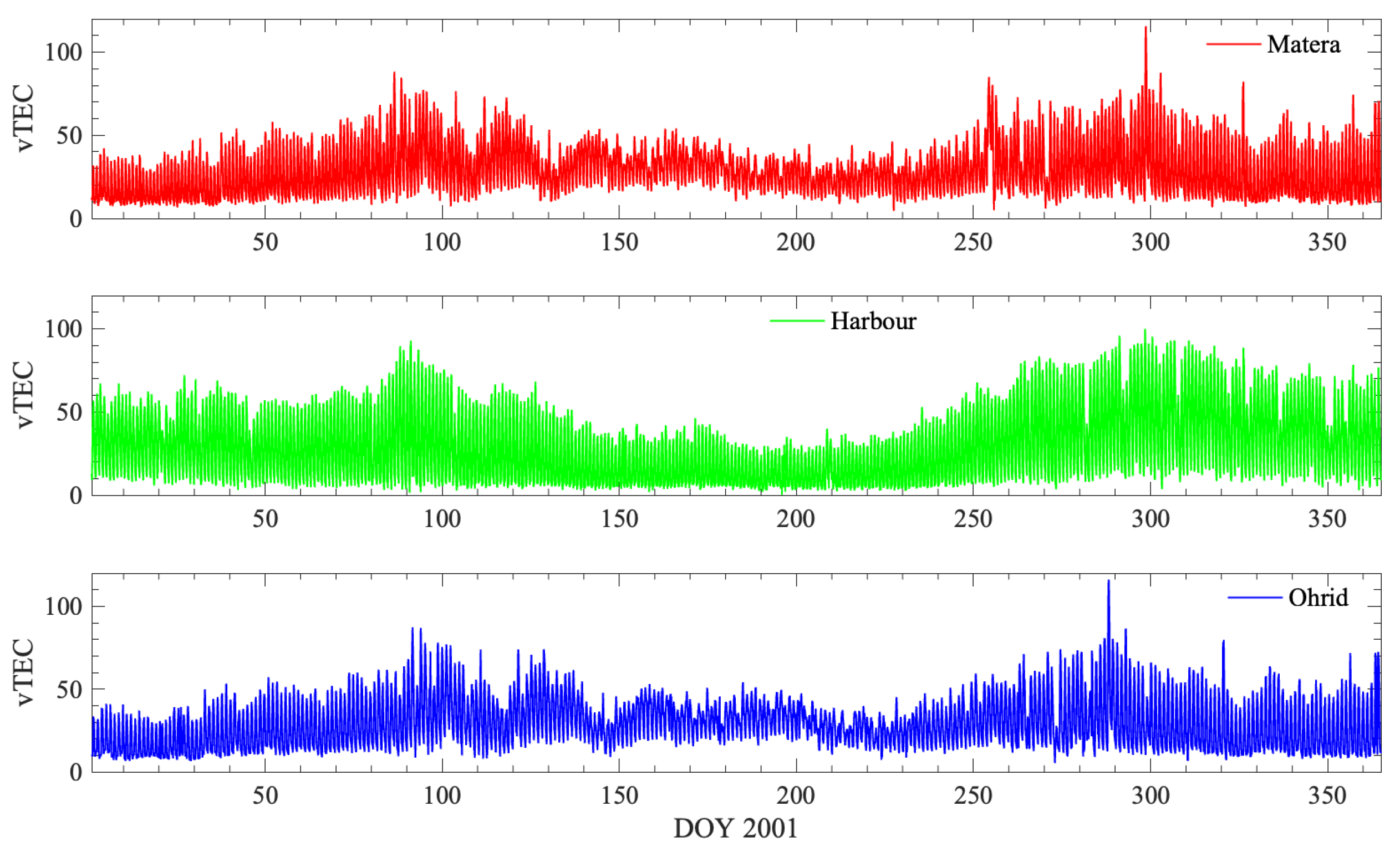
The differences in the behaviour of the LIM on the top of the three locations is evident at a glance in Figure 1, where the raw time series are directly reported. The dynamics of Matera (red) and Ohrid (blue) are very similar, while the vTEC time series on the top of Harbour (green) exhibits considerably different behavior, even if periods of maxima and minima within the year coincide.
2.2. Empirical Mode Decomposition (EMD)
The behavior of the vTEC series at different time scales is inspected via empirical mode decomposition (EMD, see for instance, [15]), through which is decomposed into a sum of a certain number of components ():
Note that in (1), the set of time scales () depends on the collection of values () of the decomposed time series, i.e., it depends on y in a functional way, as mimicked by ; this is because EMD is a data-driven method in the sense that both the form of the functions () and the characteristic scale () of each depend functionally on (this is also what means in Equation (1)). This is not, for instance, a feature of Fourier or wavelet decomposition, in which the period or the scale of the components is determined based on the size of the time-series domain.
Larger scales (s) correspond to slower modes:
as the larger the considered scale, the slower the mode, on average (as denoted by in (2)).
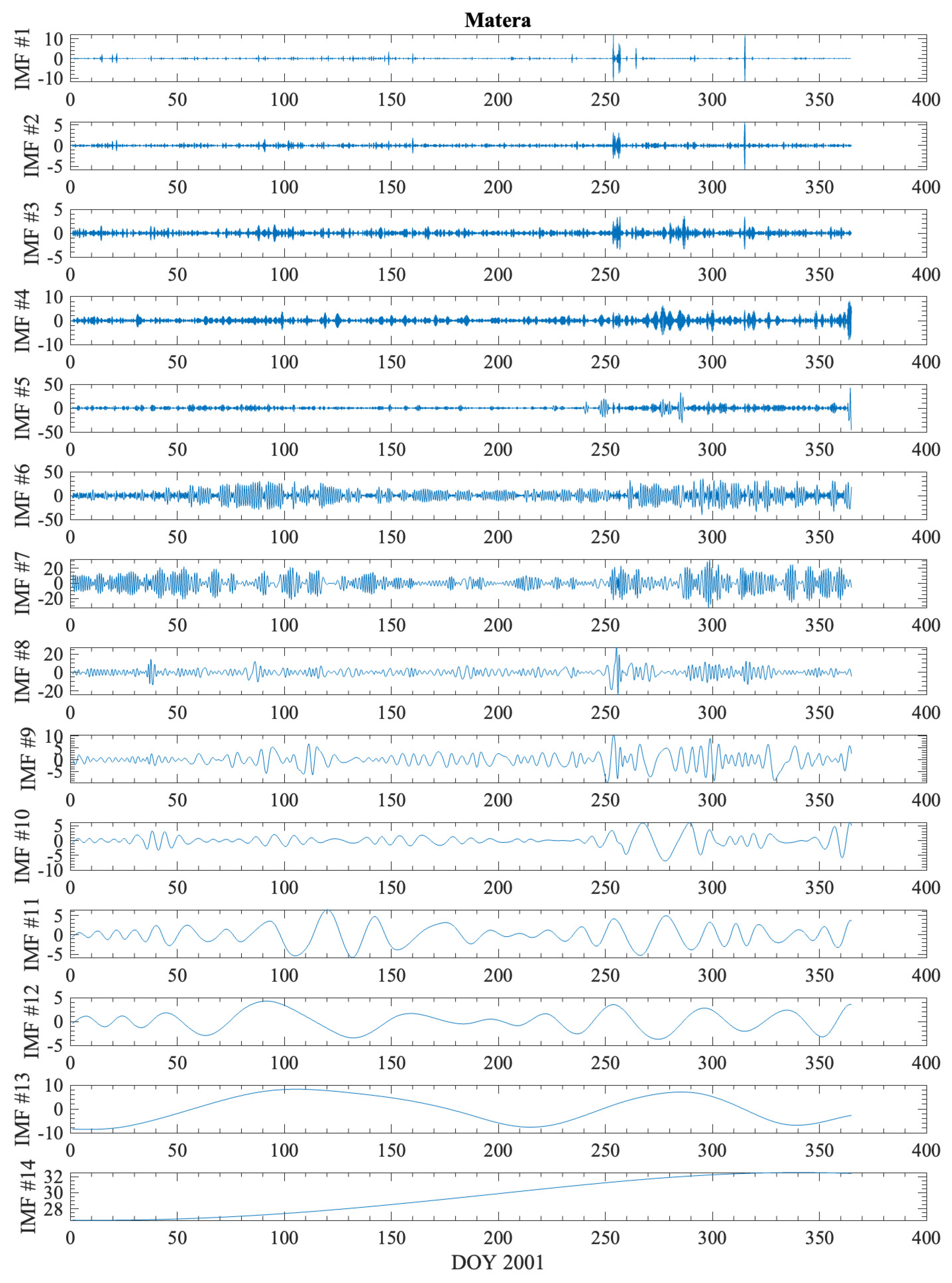
In order to get a pictorial idea of the components () into which the EMD splits the time series at hand, Figure 2 reports the different components for the time series on the top of the Matera GNSS station.
After decomposition (1), a “-cumulative partial time series” () is defined as the sum of the components () with a characteristic time scale smaller than or equal to , i.e., neglecting the modes pertaining to scales larger than :
Of course, this definition makes depend functionally on precisely as each , but this “square bracket dependence” is not highlighted in (3) in order to keep notations reasonably simple.
In the the time series, the original is considered, and all time modes “slower than” in the sense of Equation (2) are discarded. Therefore, the time series is the vTEC without the slow modes, and the scale pertains to the slowest admitted mode. If is the largest time scale admitted in the modes ) in (1), clearly, one may write
As the functions () are calculated, each of them may undergo an embedding procedure applied to the whole vTEC time series reported in [9], as well as the subsequent calculation of and . The main difference here is that this analysis of “chaos degree” and predictability of the LIM is performed at each different time scale () for each (see also [11,12]). The embedding procedure à la Grassberger–Procaccia [10], applied to the partial series () determines a trajectory () moving through an dimensional real space:
which represents the evolution of a suitable FDDS and produces the -resolved vTEC (). This trajectory () lives in a phase space ( of dimension) . As underlined by the bracket in , the dimension of the FDDS also depends on the time scale () because observing the LIM at different time resolutions, the system may look like different dynamical systems, with many or few dynamical variables, so that each has a different dimension.
The coarse graining of defines the Hausdorff dimension of the curve, which is well approximated by the correlation dimension of (see [9,10]), namely ( for simplicity). This dimension () is, in practice, the fractal dimension of the attractor containing , where the FDDS dynamics live. As discussed in [9], is bounded from above by
the closer it is to 1, the more regular the dynamics of the FDDS; for , the FDDS becomes more chaotic as approaches ; for , the FDDS is simply stochastic.
Following the prescriptions proposed in [10], the calculation of the Kolmogorov entropy rate () is applied to the single- time series (), i.e., to its -embedded version (), yielding a value of , representing the rate at which the coarse-grained version of is located less precisely than on bit, i.e., the time () after which the position () is known less precisely than of one bit. This time () is understood as the predictability time horizon of the FDDS. For , the FDDS is fully unpredictable, while for , it is completely deterministic. Our FDDS will shows a finite value of , indicating the typical finite predictability behaviour of a chaotic system.
Once the -FDDS characteristics () are calculated as functions of the time scale (), it is possible to draw physical conclusions considering those functions (). In particular, the number of dynamical degrees of freedom of the LIM as a function of the time scale, as well as degree of chaos of their dynamics, may highlight critical scales in these complex dynamics as changes in the behaviour of take place in the correspondence with changes in the value of . We report on this further in our analysis presented in Section 3. In the case reported in Figure 3, the pseudospectrum
is plotted, where is the standard deviation for the set of values of the time series of the single- components in (1) (). This pseudospectrum is useful because its dependence on corresponds approximately to the value of the Fourier spectrum of the from which the are calculated at a frequency of . Directly using the pseudospectrum instead of the Fourier spectrum is motivated by its availability once EMD is performed and by the ease of comparison with the other results obtained via the same functions. In Figure 3 and in all the subsequent analysis, components with approximately are considered, even if TEC variations with time scales of 5–20 min are linked to atmospheric waves; these components are of particular interest with respect to ionospheric dynamics. The reason to disregard those important short time scales here is related to the calculation of the correlation integrals. The latter can be affected by high-frequency contents of the time series. For this reason, modes () whose time scales are below one order of magnitude the time resolution, i.e., , are excluded. Components () can definitely be interesting in terms of ionospheric dynamics, and surely, their behaviour deserves further study, as well as additional investigation of parameters related to irregularities and radio scintillation. Moreover, the vTEC time series processed here are the result of a “calibration procedure” [16] that employs dual-frequency carrier-phase and code-delay GNSS observations related to the total electron content (TEC) along the satellite–receiver line of sight. As a consequence, the obtained vTEC is a linear combination of many TEC measurements, each including some random instrumental and processing errors. The exclusion of those high-frequency contributions () eliminates this additive, purely stochastic process resulting from calibration.
Before moving to results, it is of use to recall the formulae due proposed by Grassberger and Procacci and used in [9] for the whole yearly time series and adapted here to treat the motions () in . The central quantity of all the calculations is the correlation integral () pertaining to the relationship between two points ( and in ) along the trajectory of the FDDS, separated by an -dimensional distance equal to r:
In (6), the number of times considered is N; hence, the points of the trajectory () are , corresponding to “an enormous number” () of points. In practice, (6) represents the number of trajectory points closer than r to each other, which is normalized with respect to the number of point couples ().
Once is calculated as in (6) for the -dimensional FDDS, and are calculated as proposed by Grassberger and Procaccia [10]:
The expression of in (7) qualifies it as the Hausdorff dimension of the r-coarse-grained trajectory () within , while the expression of indicates that for each FDDS, one has to calculate for various tentative embedding dimensions (n), selecting as the value of n for which the growth of reaches a plateau (see [9,10] for more details).
As a concluding remark, it is worth stressing again that all the quantities calculated by embedding the -limited time series () are constrained by the limit relationship (4). As the -limited time series includes all ,
where and are the correlation dimension and Kolmogorov entropy rate obtained by embedding the whole original time series () into a suitable m-dimensional FDDS, respectively. Therefore, the topological characteristics of the FDDS, i.e., of the -limited that includes all the -fixed components (1), are simply those of the undecomposed (m, and of Matera are the same as those found in [9]).
3. Results
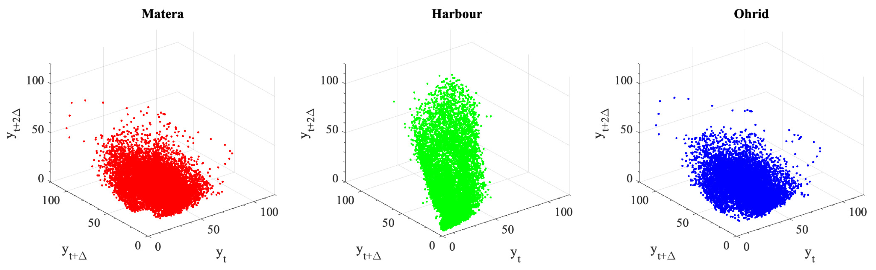
Figure 4 reports the results of the embedding procedure described in [9], applied to the time series analysed here and shown in Figure 1, where the trajectory () associated with the whole time series () is reported in the space for Matera, Harbour and Ohri. These trajectories are simply the time vector series , i.e., their components are suitably delayed copies of the original observed time series . As explained in [9] and references therein, if the FDDS equivalent to that yielding is diffeomorphic to the vector of the delayed copies of the time series, it is possible to visualise the FDDS trajectories throughout the phase space. The lag reduces the -delayed self-mutual information of the to less than bit.
The three s in Figure 4 all have an embedding dimension of 3. The result represented in Figure 4 is consistent with the appearance of the time series in Figure 1, with an apparently more elongated and flatter region of attraction for the low-geographic-latitude LIM on Harbour with respect to those on Matera and Ohrid.
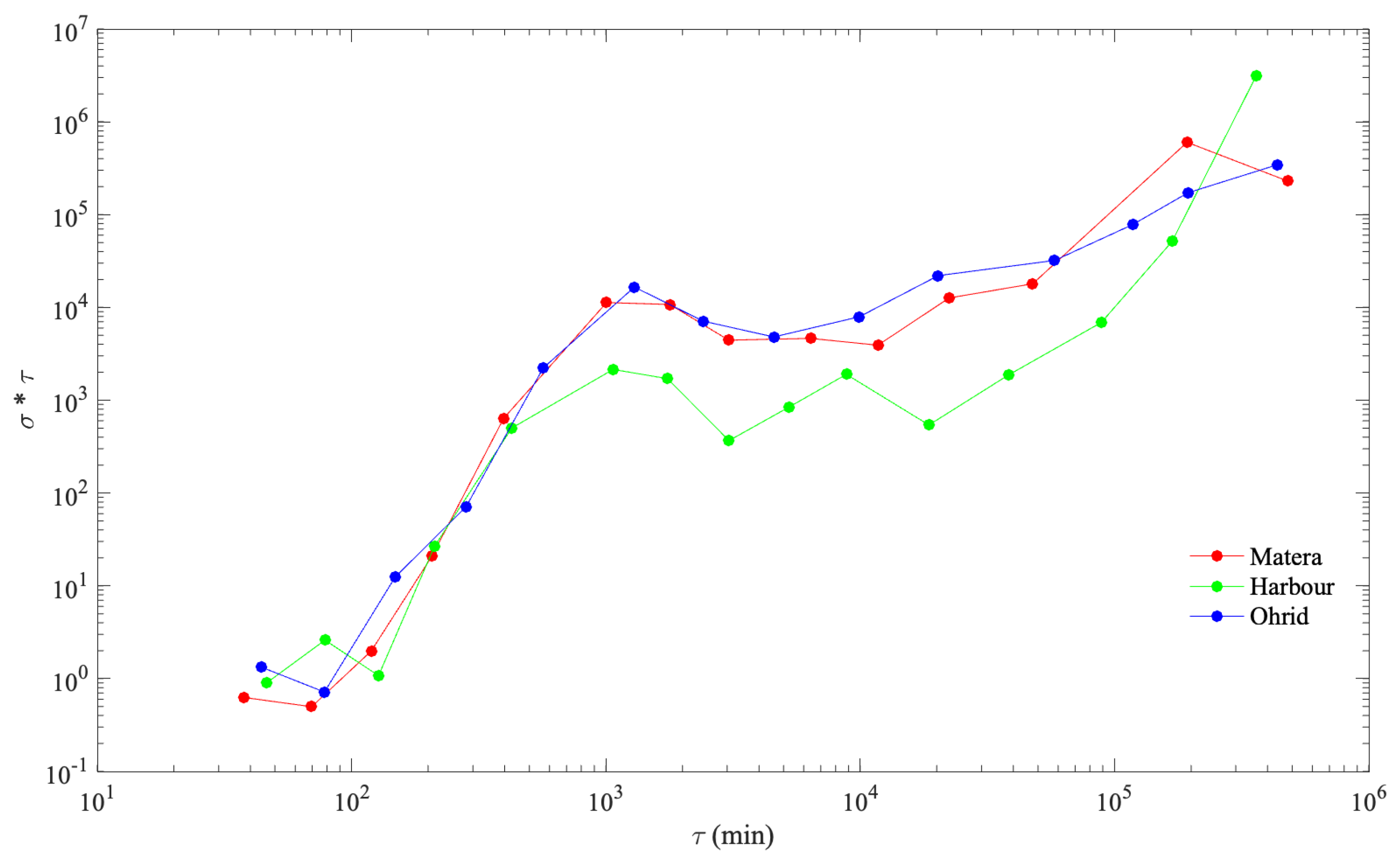
The first notable result of the decomposition (1) is the behaviour with of the pseudospectrum () calculated as in (5) and reported in Figure 3, where the pseudospectrum is shown for the three time series (, and ). With respect to the general behaviour, the three pseudospectra are rather similar, while in the details, they differ quite a bit, with a stricter resemblance between Matera and Ohrid than relative to Harbour. Besides the differences among the three curves, one observes a considerable change in regime at , which is close to the corresponding to the length of one terrestrial day. The slopes of for and for are different; in particular, the short time components () exhibit steeper growth with than the slower ones. Moreover, a local maximum of appears at . The pseudospectrum of the Harbour vTEC is lower than that of Matera and Ohrid vTECs, and for , the growth associated with seems “less monotonic”, with a local maximum at about . Whether this maximum at a scale of about days has a physical meaning or not and what that meaning might be deserve a much deeper study consulting more statistics of the GNSS stations. Figure 3 shows the two slope regimes separated by the time scale of the Earth’s rotation.
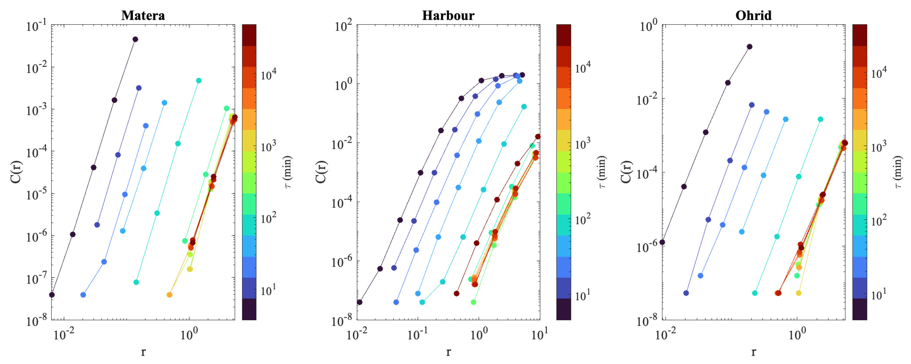
Once the -limited series () are composed, (6) is applied to define the correlation integrals (), as reported in Figure 5, where the curves () correspond to , and different colours correspond to different values of the time-scale . The value of varies as a function of for a fixed r, as do the characteristics of the FDDS, as they depend on according to Formula (7). Again, the similarity between the LIM on the top of the two mid-latitude stations (Matera and Ohrid) and the difference with respect to the low-latitude station (Harbour) are evidenced in Figure 5.
Once the quantities are calculated, it is possible to explore the degree of chaoticity of the different FDDSs by calculating the dimension () and their predictability by calculating the entropy rate (), applying the Grassberger–Procaccia formulae (7).
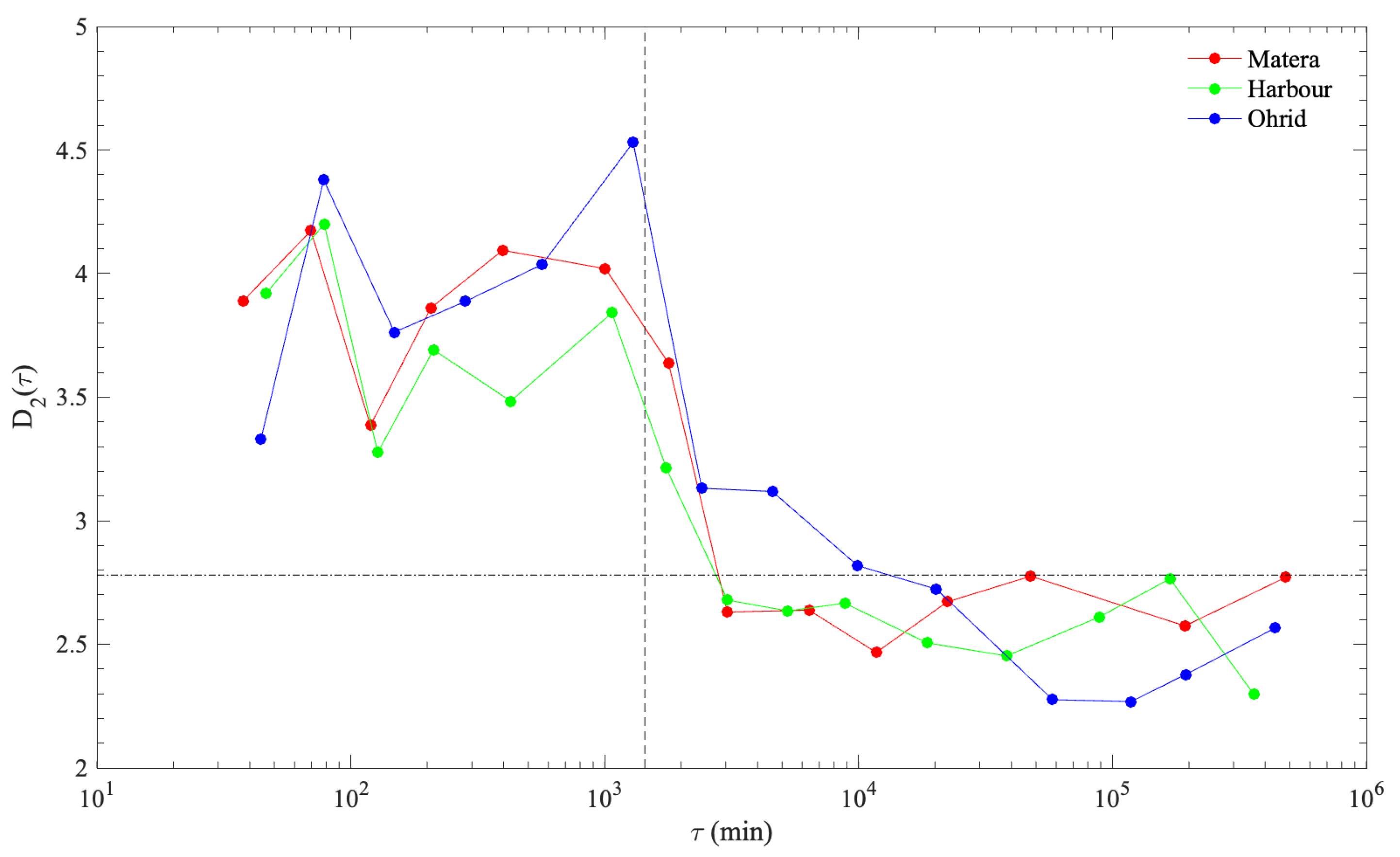
The dependence () is plotted in Figure 6 for the three GNSS stations. The 1-day scale break appears again, with (slightly) different behaviour for the three different stations. The similarities between the two mid-latitude stations and the difference between those two and the low-latitude station appear to be less important here than in the pseudospectra shown in Figure 3. It can be concluded that the representation of the LIM by FDDSs is limited to scales smaller than , reaching values higher than 3; therefore, excluding scales larger than , the effective dynamical system representing the local ionosphere needs more than three independent dynamical variables to be described. In addition to , when including much slower s in , rapidly decreases, reaching almost for Matera, nearly for Ohrid and as low as for Harbour. This result is in agreement with what is illustrated in Figure 4, where the three whole time series (, and ) appear to be embedded in a three-dimensional FDDS. Moreover, as apparent in the same Figure 4, the degree of chaos at Harbour is (slightly) lower than at the mid-latitude LIMs.
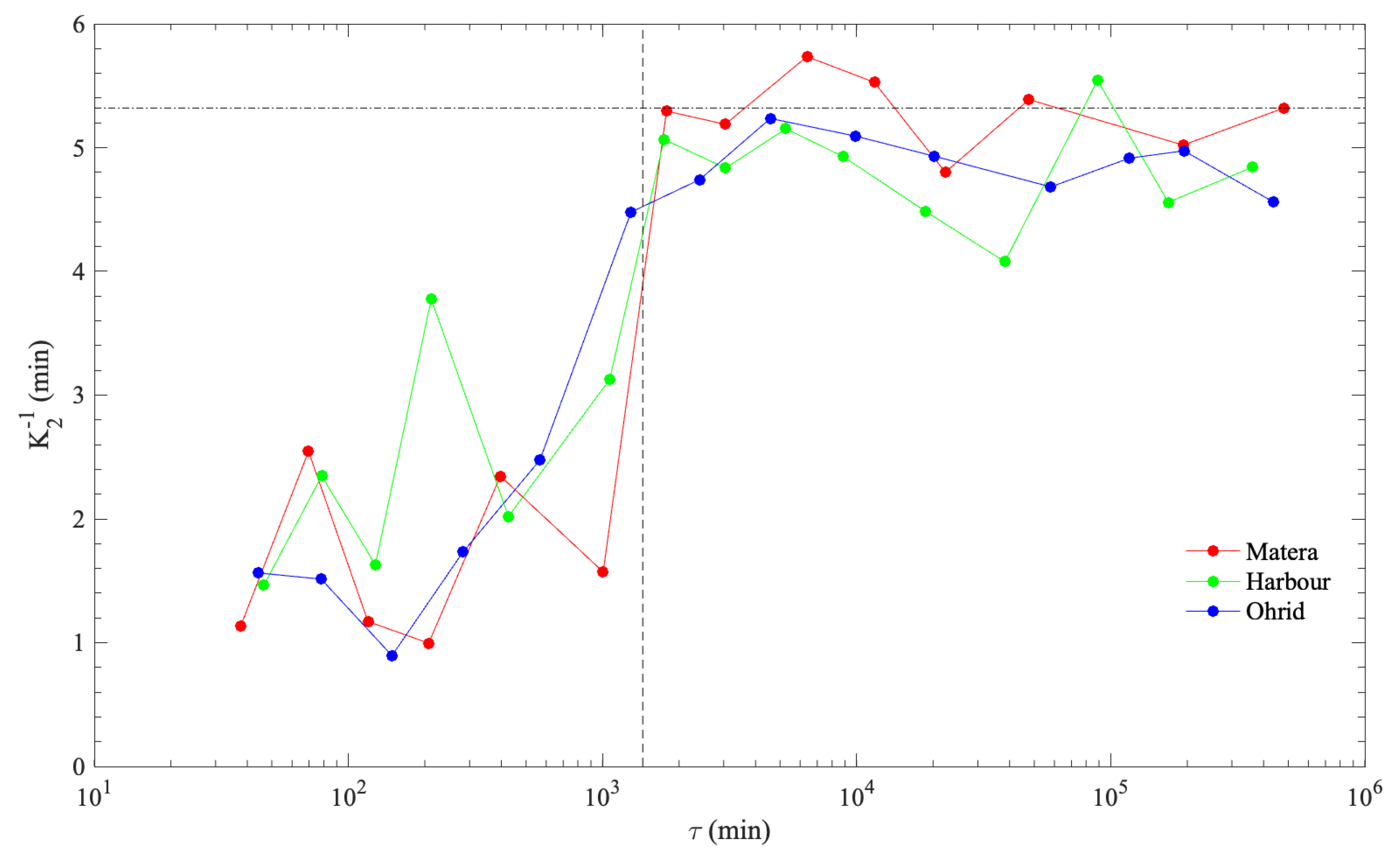
The dynamical behaviour of the vTEC on the top of the three considered GNSS stations, appearing to be richer and more chaotic at shorter than at longer time scales, with a drastic separation into and , is also reflected by the -dependent predictability time horizon (), as represented in Figure 7. For -limited dynamics with , the highest value of is about , corresponding to on the top of Harbour, and generally remaining below 3 min. This predictability time horizon grows abruptly by as much as for , increasing to almost 6 min for on the top of Matera.
The dependence of and on reported in Figure 6 and Figure 7 not only shows a qualitative transition between and but also some kind of “saturation” for . This may sound surprising, mainly for , as increasing values correspond to components with longer “periods”, namely increased predictability. However, here, we are calculating and for the FDDS equivalent to in Equation (3), which represents the cumulative contributions of . The series still encodes the chaotic properties of all the time scales (), and increasing does not exclude those highly irregular components, preventing the indefinite growth of the predictability time horizon beyond saturation.
4. Discussion and Conclusions
Herein, we present here a step forward in describing the local ionospheric medium (LIM) in a brand-new and deeply dynamic theoretical manner.
Data-conditioned representations of the LIM are traditionally empirical models constructed through the collection of huge datasets referring to suitably assorted ionospheric locations and conditions [17,18]. Despite their success in describing the average climatological behaviour of systems, they are neither able to take into account suddenly developing irregularities nor focus on theoretical explanations of LIM dynamics. In this study, we interrogated ionospheric data in order to evaluate quantities pointing to describe the LIM as a dynamical system from scratch. This attitude, on the one hand, allows results to be obtained based on reality rather than (even physically reasonable) assumptions and, on the other hand, the LIM to invoke representations with the goal of tracing detailed physical mechanisms.
The physical data representing LIM evolution are time series of the vertical total electron content (vTEC) on the tops of three considered stations. Our aim was to describe the LIM dynamics as those of a finite dimensional dynamical system (FDDS). These time series are embedded into a suitable phase space according to the Grassberger–Procaccia procedures [10], and the Hausdorff dimensions of their strange attractors, as well as the Kolmogorov entropy rate, are calculated.
In [9], raw yearly time series of a vTEC () were analysed so to ensure an equivalent FDDS of trajectory , ; here, we decompose time series into empirical modes (), each with a characteristic time scale (), then use them to define -limited time series () as in (3) so that includes all the modes () from faster than . Each of the -limited vTEC series () is ultimately embedded as , and the dynamical proxies () of the scale-dependent embedding dimension, correlation dimension and Kolmogorov entropy rate are calculated. Excluding from all the slower components () reveals the faster motion details of the LIM dynamics. In fact, slower modes tend to have larger amplitudes, masking the faster, weak-amplitudevariability.
The interest in assigning a distinct equivalent FDDS to each is twofold. On the one hand, the LIM may look very different at different time scales; identifying the dependence of the dynamical quantities (, and ) on time scales rephrases this statement in a precise and quantitative way. On the other hand, values of discriminating different behaviours of , or should represent characteristic time scales of the local ionospheric physics that are useful in singling out important processes influencing the LIM.
Our results suggest that (1) there is an expected similarity between the vTEC dynamics above Matera and Ohrid, while the vTEC above Harbour behaves a slightly differently, indicating hemispheric variation and (2) a time scale of about 1 day represents a threshold at which the characteristics of the FDDS change.
The take-home message of these results is that multi-scale analysis calculating the quantities of , and unveils very important new details about LIM dynamics as represented by vTEC time series. According to the findings presented here, the LIM is a complex dynamical system that has finite dimensional representations depending on the time scale. The smaller the time scale (), the higher the number of dynamical variables necessary to describe the LIM at that scale. Moreover, all FDDSs representing the LIM evolve along chaotic trajectories (), filling -dimensional attractors with and increasing with smaller scales; therefore, the smaller the , the more chaotic the LIM-equivalent FDDS. Lastly, the predictability time horizon () decreases with smaller scales; therefore, the smaller the , the more unpredictable the LIM-equivalent FDDS. The picture presented herein is that of a chaotic and unpredictable system at all time scales, although it is more chaotic and less predictable in its fast modes than in its slow modes. When examining the LIM at a more detailed time scale, one is able to distinguish the action of independent dynamical variables that are undetectable at large time scales, i.e.,
and one finds that such “fast modes” are invisible at large s, resulting in a higher level of chaos, i.e.,
and unpredictability, i.e.,
Equations (9)–(11) refer to the “trends” of , and , while oscillations and local peaks and valleys with may appear. These tendencies abruptly increase at about . In accordance with Earth’s rotation period, and decrease abruptly with increasing , while exhibits a sudden increase. This has a precise physical meaning: sunlight is the natural time scale that separates fast modes from slow modes in the vTEC dynamics, which sounds very reasonable due to the role played by insolation in ionospheric physics.
All the conclusions just reported apply slightly differently to the two northern hemisphere, mid-latitude locations than to the southern hemisphere location examined herein, with the caveat that such a difference is an interhemispheric difference. However, geomagnetic latitude should be expected to influence the detailed behaviour of , and , probably more than other local conditions. This calls for a systematic extension of the present study in order to confirm our findings.
Based on the results reported in [9] and those presented here, our attempt to construct an FDDS equivalent to the local ionospheric medium portrays the system as chaotic and unpredictable to a certain extent, appearing richer and less predictable in its fast modes than in its slow modes, corresponding to the period of the Earth’s daily rotation, i.e., the separation time scale. The details of these findings depend on the location under consideration. The emergence of this complex behaviour is witnessed here for yearly time series () of vTEC above the three investigated stations. Therefore, we suggest (1) an extension of this analysis to many more locations in order to more consistently how the , and vary with geomagnetic coordinates; (2) time-limited studies concentrating on geomagnetically homogeneous periods in order to determine how the multi-scale complexity of vTEC series depends on present geomagnetic activity, as well as techniques compatible with shorter time series and the expression of FDDS quantities as functions of the present (e.g., ; see [19]), which can help to monitor LIM complexity above a given location throughout the various phases of a geomagnetic storm [20].
The very difficult challenge of this line of research is to pass from knowledge of for an FDDS to a possible set of m-coupled ordinary differential equations:
where represent independent dynamical variables moving along a -dimensional attractor within , with a Kolmogorov entropy rate [21]. Mapping into the suitable system (12) is all but a trivial challenge in general, and in the case of the LIM, one has a different FDDSs, i.e., a different (12) at each scale () and probably also differing under the various geomagnetic conditions. The theoretical sense of arriving at a system like (12) for the LIM is to produce, for the ionosphere, what the Lorenz system equations [22] represent for the physics of the neutral atmosphere.
In principle, within a geomagnetically homogeneous period, after collecting all the dynamics (s) and finding what (12) looks like for ,
(that is, the Lorenz equivalent of the LIM system at scale (τ)), keeping track of the function , (13) is an analytical/numerical predictor of the -limited vTEC within the time interval under consideration. Despite the loftiness of the goal, this program, when fully pursued, may represent a striking breakthrough in ionospheric modelling.
Author Contributions
Conceptualization, M.M. and S.M.R.; methodology, T.A. and G.C.; software, T.A.; validation, M.M., Y.M.-O. and S.M.R.; formal analysis, M.M. and T.A; data curation, Y.M.-O.; writing—original draft preparation, M.M.; writing—review and editing, Y.M.-O., S.M.R., T.A. and G.C. All authors have read and agreed to the published version of the manuscript.
Funding
T.A. acknowledges funding from the “Bando per il finanziamento di progetti di Ricerca Fondamentale 2022” of the Italian National Institute for Astrophysics (INAF)—Mini Grant: “The predictable chaos of Space Weather events”.
Institutional Review Board Statement
Not applicable.
Informed Consent Statement
Not applicable.
Data Availability Statement
The vTEC data series were obtained from the ICTP Calibrated GNSS TEC data service and are available at https://arplsrv.ictp.it, accessed on 10 January 2022.
Conflicts of Interest
The authors declare no conflicts of interest.
References
- Kelley, M.C. The Earth’s Ionosphere—Plasma Physics and Electrodynamics; Elsevier Inc.: Amsterdam, The Netherlands, 1989; ISBN 978-0-12-404013-7. [Google Scholar]
- Materassi, M.; Forte, B.; Coster, A.; Skone, S. (Eds.) The Dynamical Ionosphere—A Systems Approach to Ionospheric Irregularity; Elsevier Inc.: Amsterdam, The Netherlands, 2020; ISBN 978-0-12-814782-5. [Google Scholar]
- Goodman, J.M. The Ionosphere. In Space Weather & Telecommunications; The International Series in Engineering and Computer Science; Springer: Boston, MA, USA, 2005; Volume 782. [Google Scholar] [CrossRef]
- Hunsucker, R.D. Radio Techniques for Probing the Terrestrial Ionosphere; Springer Science & Business Media: Berlin/Heidelberg, Germany, 2013; Volume 22. [Google Scholar]
- Lilensten, J.; Blelly, P.L. The TEC and F2 parameters as tracers of the ionosphere and thermosphere. J. Atmos. Sol.-Terr. Phys. 2002, 64, 775–793. [Google Scholar] [CrossRef]
- Bolzan, M.J.A.; Tardelli, A.; Pillat, V.G.; Fagundes, P.R.; Rosa, R.R. Multifractal analysis of vertical total electron content (VTEC) at equatorial region and low latitude, during low solar activity. Ann. Geophys. 2013, 31, 127–133. [Google Scholar] [CrossRef]
- Chandrasekhar, E.; Prabhudesai, S.S.; Seemala, G.K.; Shenvi, N. Multifractal detrended fluctuation analysis of ionospheric total electron content data during solar minimum and maximum. J. Atmos. Sol.-Terr. Phys. 2016, 149, 31–39. [Google Scholar] [CrossRef]
- Kumar, K.S.; Kumar, C.V.A.; George, B.; Renuka, G.; Venugopal, C. Analysis of the fluctuations of the total electron content (TEC) measured at Goose Bay using tools of nonlinear methods. J. Geophys. Res. 2004, 109, A02308. [Google Scholar] [CrossRef]
- Materassi, M.; Alberti, T.; Migoya-Orué, Y.; Radicella, S.M.; Consolini, G. Chaos and Predictability in Ionospheric Time Series. Entropy 2023, 25, 368. [Google Scholar] [CrossRef] [PubMed]
- Grassberger, P.; Procaccia, I. Characterization of strange attractors. Phys. Rev. 1983, 50, 346. [Google Scholar] [CrossRef]
- Alberti, T.; Consolini, G.; Ditlevsen, P.D.; Donner, R.V.; Quattrociocchi, V. Multiscale measures of phase-space trajectories. Chaos Interdiscip. J. Nonlinear Sci. 2020, 30, 123116. [Google Scholar] [CrossRef] [PubMed]
- Alberti, T.; Donner, R.V.; Vannitsem, S. Multiscale fractal dimension analysis of a reduced order model of coupled ocean-atmosphere dynamics. Earth Syst. Dyn. 2021, 12, 837–855. [Google Scholar] [CrossRef]
- Rawer, K. Meteorological and Astronomical Influences on Radio Wave Propagation; Landmark, B., Ed.; Academic Press: New York, NY, USA, 1963; pp. 221–250. [Google Scholar]
- Consolini, G.; Alberti, T.; De Michelis, P. On the Forecast Horizon of Magnetospheric Dynamics: A Scale-to-Scale Approach. J. Geophys. Res. 2018, 123, 9065–9077. [Google Scholar] [CrossRef]
- Huang, N.E.; Shen, Z.; Long, S.R.; Wu, M.C.; Shih, H.H.; Zheng, Q.; Yen, N.-C.; Tung, C.C.; Liu, H.H. The empirical mode decomposition and the Hilbert spectrum for nonlinear and non-stationary time series analysis. Proc. R. Soc. Lond. Ser. A 1998, 454, 903. [Google Scholar] [CrossRef]
- Ciraolo, L.; Azpilicueta, F.; Brunini, C.; Meza, A.; Radicella, S.M. Calibration errors on experimental slant total electron content (TEC) determined with GPS. J. Geod. 2007, 81, 111–120. [Google Scholar] [CrossRef]
- Bilitza, D. IRI the International Standard for the Ionosphere. Adv. Radio Sci. 2018, 16, 1–11. [Google Scholar] [CrossRef]
- Radicella, S.M. The NeQuick model, genesis, uses and evolution. Ann. Geophys. 2009, 52, 417–422. [Google Scholar]
- Alberti, T.; Faranda, D.; Lucarini, V.; Donner, R.V.; Dubrulle, B.; Daviaud, F. Scale dependence of fractal dimension in deterministic and stochastic Lorenz-63 systems. Chaos Interdiscip. J. Nonlinear Sci. 2023, 33, 023144. [Google Scholar] [CrossRef] [PubMed]
- Ogunsua, B.O.; Laoye, J.A.; Fuwape, I.A.; Rabiu, A.B. The comparative study of chaoticity and dynamical complexity of the low-latitude ionosphere, over Nigeria, during quiet and disturbed days. Nonlinear Process. Geophys. 2014, 21, 127–142. [Google Scholar] [CrossRef]
- Brunton, S.L.; Proctor, J.L.; Kutz, J.N. Discovering governing equations from data by sparse identification of nonlinear dynamical systems. Proc. Natl. Acad. Sci. USA 2016, 113, 3932–3937. [Google Scholar] [CrossRef] [PubMed]
- Lorenz, E.N. Deterministic non periodic flow. J. Atmos. Sci. 1963, 20, 130–141. [Google Scholar] [CrossRef]
Figure 1.
The three yearly time series of vTEC during solar maximum year 2001: from the tops of the Matera, Harbour and Ohrid GNSS stations.
Figure 1.
The three yearly time series of vTEC during solar maximum year 2001: from the tops of the Matera, Harbour and Ohrid GNSS stations.

Figure 2.
The different components () into which the EMD splits the time series () plotted in Figure 1. The convention here is to count the s from the shortest value to the longest one so that .
Figure 2.
The different components () into which the EMD splits the time series () plotted in Figure 1. The convention here is to count the s from the shortest value to the longest one so that .

Figure 3.
Plot of the pseudospectrum as defined in (5) for the three time series reported in Figure 1. The remarkable feature of these plots is the break at , corresponding to the rotation period of the planet, resulting in the insolation tempo (see text for details).

Figure 4.
The three-dimensional trajectories resulting from the embedding procedure as described in [9] applied to the whole yearly time series plotted in Figure 1. Note the strong similarity between the trajectories () for Matera and Ohrid, while the LIM on the top of Harbour appears to correspond to a differently shaped attractor. See the text for details.

Figure 5.
The correlation integrals () depending on the time scale () for the three considered GNSS stations.
Figure 5.
The correlation integrals () depending on the time scale () for the three considered GNSS stations.

Figure 6.
The dependence () for the FDDS representing the LIM on the top of the three GNSS stations (Matera, Ohrid and Harbour). The horizontal dashed line represents the value of for a large value for the Matera LIM, taken as a reference; and the vertical dashed line marks the scale. See the text for details.

Figure 7.
The dependence () for the a FDDS representing the LIM on the top of the three GNSS stations (Matera, Ohrid and Harbour). The horizontal dashed line represents the value of for a large value for the Matera LIM, taken as a reference; and the vertical dashed line marks the scale. See the text for details.

Disclaimer/Publisher’s Note: The statements, opinions and data contained in all publications are solely those of the individual author(s) and contributor(s) and not of MDPI and/or the editor(s). MDPI and/or the editor(s) disclaim responsibility for any injury to people or property resulting from any ideas, methods, instructions or products referred to in the content. |
© 2024 by the authors. Licensee MDPI, Basel, Switzerland. This article is an open access article distributed under the terms and conditions of the Creative Commons Attribution (CC BY) license (https://creativecommons.org/licenses/by/4.0/).
Share and Cite
MDPI and ACS Style
Materassi, M.; Migoya-Orué, Y.; Radicella, S.M.; Alberti, T.; Consolini, G. Multi-Time-Scale Analysis of Chaos and Predictability in vTEC. Atmosphere 2024, 15, 84. https://doi.org/10.3390/atmos15010084
AMA Style
Materassi M, Migoya-Orué Y, Radicella SM, Alberti T, Consolini G. Multi-Time-Scale Analysis of Chaos and Predictability in vTEC. Atmosphere. 2024; 15(1):84. https://doi.org/10.3390/atmos15010084
Chicago/Turabian StyleMaterassi, Massimo, Yenca Migoya-Orué, Sandro Maria Radicella, Tommaso Alberti, and Giuseppe Consolini. 2024. "Multi-Time-Scale Analysis of Chaos and Predictability in vTEC" Atmosphere 15, no. 1: 84. https://doi.org/10.3390/atmos15010084
Note that from the first issue of 2016, this journal uses article numbers instead of page numbers. See further details here.