

Comparative Analysis of Starlight Occultation Data Processing

1
China Research Institute of Radiowave Propagation, Qingdao 266107, China
2
Deep Space Exploration Laboratory, Beijing 100041, China
*
Author to whom correspondence should be addressed.
Atmosphere 2023, 14(12), 1818; https://doi.org/10.3390/atmos14121818
Submission received: 16 October 2023
/
Revised: 2 December 2023
/
Accepted: 11 December 2023
/
Published: 13 December 2023
(This article belongs to the Section Atmospheric Techniques, Instruments, and Modeling)
Abstract
:In order to improve the inversion accuracy of stellar occultation data and to provide a reference for the selection of inversion methods with higher accuracy in the future, this study compared and analyzed the inversion effects of two different methods on the same set of data, which are the effective cross-section method and the onion-peeling method, respectively. Firstly, the inversion principle of the effective cross-section method is introduced in detail. The regularisation parameters and screening conditions for the observation data in the inversion process were clarified based on the ozone observation characteristics. Second, the algorithm was applied to invert the GOMOS observational data from 1 December 2002. The atmospheric radiative transmittance obtained from the observations was filtered, and the inversion results were compared with those obtained using the onion-peeling method. Third, the errors in the height distribution obtained by both methods were calculated using the GOMOS secondary results from 1 December 2002 as the reference value. Finally, the inversion errors of other trace components were computed to further validate the accuracy of the two methods. The results demonstrate that the effective cross-sectional method is more accurate for the inversion of ozone, particularly in low-altitude regions affected by refraction. The method achieved a maximum error of 1.2%, with an apparent magnitude of 2, an effective temperature greater than 10,000 K, and a regularisation parameter of 1015. Furthermore, when applying the same method to the inversion of nitrogen trioxide and calculating the error, it was observed that the results of both methods were comparable at altitude of 30–60 km, with an error value ranging from 0 to 2%. However, at approximately 25 km, the inversion accuracy of the onion-peeling method surpassed that of the effective cross-sectional method. This research provides a theoretical foundation for further investigation of the stellar occultation inversion method and enhancing the accuracy of inversions.
1. Introduction
The stellar occultation technique is crucial for studying the atmospheres of planets such as Earth [1,2], Mars [3,4,5], and Venus [6]. This technique indirectly measures the stellar spectra to obtain a global distribution of planetary atmospheric trace components. The inversion results were then used to analyse the composition of planetary atmospheres, track evolutionary trends, and develop atmospheric models. Therefore, it is important to accurately invert the vertical profiles of the trace components from the measured spectra to ensure inversion quality. Currently, the quality of starlight occultation inversion is affected by the occultation mode, stellar brightness, stellar temperature, and occultation inclination. These factors are also significant for screening the inversion data.
According to the research, five main inversion methods for stellar occultation data have been identified [7]. These methods are as follows: the onion-peeling method, Tikhonov regularization method, Tikhonov-type regularization, maximum a posteriori (MAP) estimation, and the classical MAP method. Methods that rely on a priori information are limited, because such information is not available at high altitudes [8]. The Tikhonov regularisation method has a predetermined vertical resolution, whereas the resolution of the MAP method depends on the noise level. The MAP method is suitable when the data are heavily contaminated by noise. However, it cannot currently be used because of the ozone variability, unless the satellite observatory site coincides with the ozone observatory. Methods 2 and 3 offer grid-independent forms that are crucial for highly inhomogeneous measurements.
This section focuses on the two methods used in this study.
- Onion-peeling method: This method does not require any prior information and provides good vertical resolution. However, it is observed that the inversion of faint star data is noisy at low altitudes due to the strong influence of the observed star source, such as the apparent star. Therefore, it is preferable to use the observed data of bright stars for the inversion.
- Tikhonov-type regularization: Regularization, in linear algebra theory, refers to the fact that an ill-posed problem is usually defined by a set of linear algebraic equations, and that this set of equations usually stems from an ill-posed inverse problem with a large condition number. A large condition number means that rounding or other errors can seriously affect the outcome of the problem. As stellar occultation data inversion causes ill-posed problems, Tikhonov proposed using the A, method, called the Tikhonov matrix (Tikhonov matrix) [8]. Its advantage is its simplicity, but its disadvantage is that resolution is not taken into account and the optimal inversion wavelength depends on the spectral signal, as well as the tilt of the occultation.
In our previous research, we utilised the onion-peeling method, a single inversion method, to accurately invert the oxygen components [9,10,11]. This study investigates a new inversion algorithm, the effective cross-sectional method, to achieve the high-precision inversion of components in near-space. The structure of this paper is as follows: Section 2 introduces the principle of the effective cross-sectional method; Section 3 presents a comparison of inversion results and errors between the effective cross-sectional method and onion-peeling method; and Section 4 provides the conclusions and outlook.
2. Inversion Methodology
This section explores the principles of the effective cross-sectional method. It is employed to determine the atmospheric component density through a two-step process. The first involves using the observed transmittance to derive the line density along the line-of-sight direction, known as spectral inversion. The second step utilises the line density to obtain the number density profile, which is referred to as vertical inversion. These two steps effectively connect spectral inversion and vertical inversion by utilising the physical quantity of the effective cross-section. Consequently, this method is referred to as the effective cross-sectional method.
According to Beer’s law, Equation (1) [12] defines T as the atmospheric radiant transmittance, which is determined by wavelength and height. is optical depth, is density of atmospheric composition, is absorption cross-section, s is the light transmission path during an occultation event, is effective absorption cross-section, and is column density along the line of sight. By utilizing Equation (1) and T, the for different heights can be calculated. Consequently, with a known effective cross-section , the column density can be calculated. The absorption cross-section at the tangent point can be read from the observation data. The above implements the first step of the algorithm. Assuming that the Earth has local spherical symmetry, Equation (2) [12] can be used to inversely obtain the vertical density profile of component j. This completes the second step of the algorithm.
In order to avoid the error caused by the observed absorption cross-sections, we use the and , obtained from Equations (1) and (2), respectively, and bring them into Equation (3) [12] to calculate the effective absorption cross-sections corresponding to different heights of the tangent points. Finally, the obtained effective absorption cross-sections are brought into Equation (1) to obtain the new . Based on the density results obtained with different numbers of cycles, we obtain the following conclusions, and repeat steps (1) and (2) at least once, and, at most, two times; at this point, the error is minimized.
Here are the specific calculations for this two-step process.
The line density at tangent height z of an occultation event can be obtained using Formula (4) [12]:
Assuming that the vertical density is a function of successive heights (used as an alternative to onion peeling) [12]:
Combining Equations (4) and (5) allows for and to be written in matrix form [12]:
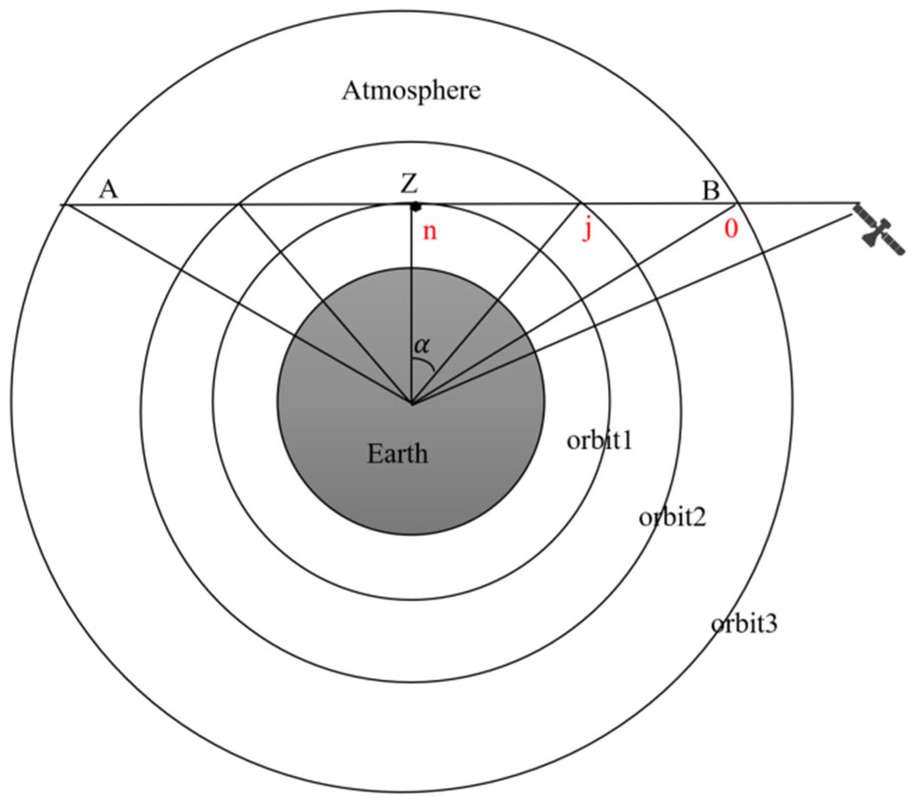
where K denotes the kernel matrix. Therefore, the core of the solution lies in the solution of the kernel matrix and line density matrix. The starlight occultation schematic is shown in Figure 1, AB is the integral effective path, Z is the height of the tangent point of the occultation event, and 0, n, and j are the occultation event stratifications.
The problem of inversion falls into the category of undesirable problems, because the measurements themselves cannot be uniquely determined. This leads to unphysical oscillations in the inversion results [13,14,15]. Moreover, the signal-to-noise ratio of the occultation measurements is strongly dependent on the apparent magnitude and effective temperature of the star, which also affect the inversion error of the vertical profile. For stars with apparent magnitudes greater than 2.5, the inversion results exhibit significant unphysical oscillations below 18 km and above 80 km. Therefore, a form of constraint must be applied to address this issue. Several solutions are currently available.
The atmosphere was divided into layers based on the measurement structure, with certain assumptions made for each layer to convert uncertainty into certainty. This discretisation process helps avoid noise or noise amplification. In this study, we assumed a linear vertical inversion in which the atmosphere was discretised into layers based on the number of measurements. The number density was then set as a function of the successive heights. This approach is similar to the onion-peeling method [9] and will not be further discussed here.
In addition, we introduce a special constraint that involves smoothing the results using a Tikhonov-type regularisation method. By utilising a priori information about the atmosphere and assuming a Gaussian noise distribution, this method provides a solution with minimal variance. Consequently, Equation (6) can be transformed into [12]:
where H denotes the height of each tangent point in Equation (8) [12].
where is a shorthand for all matrix elements divided by the square of the local altitude difference, hj = z(j − 1) − z(j). is the diagonal matrix, and the covariance matrix is generated. is related to the vertical resolution and is a regularisation parameter with a value of 1015 [16,17]. At this point, the apparent magnitude of the corresponding target star is two (other conditions are described in Section 3).
Matrices K and N are solved as follows and, from Equation (6), the density can be written as a function of the height. The derivation is as follows:
where a and b are constants related to the tangent height. This can be substituted into Equation (2) as follows:
where A is the relationship between the occultation path and tangent point; S is the effective path length of the occultation, which can be calculated based on the location of the tangent point and the coordinates of the receiving satellite position in the dataset. Z represents the height of the tangential point. For heights greater than 20 km, the light path deviation caused by refractive bending can be disregarded. This process is substituted into Equation (10) as follows:
Using Equation (6), matrix K can be obtained. After the number density was obtained, the result was substituted into Equation (3) to obtain a new effective cross-section. The effective cross-section obtained from the calculation was substituted to obtain the vertical density profile, and the cycle was repeated once to obtain the desired result.
The onion-peeling method utilises atmospheric transmittance to directly obtain the vertical profile of a component without solving the line density. The inversion principle and an accuracy analysis of this method can be found in other articles published by the author [9] and will not be presented in detail here.
3. Analysis of Results
3.1. Observation Data Sets
Global Ozone Monitoring by Occultation of Stars (GOMOS) is a medium-resolution spectrometer onboard the ESA satellite ENVISAT, launched on 1 March 2002. This instrument is dedicated to exploring the Earth’s atmosphere using the stellar occultation technique. GOMOS has accumulated observational data for over 10 years. The monitoring bands of the instrument include the following: 250–675 nm, 756–773 nm, and 926–952 nm. It measures various components, such as ozone, , and aerosols [18,19,20,21,22]. The main objective of GOMOS is to study global stratospheric ozone evolution trends and develop prediction models. The monitoring error of ozone is estimated to be 1–5% in the stratosphere at night, 10% at 20 km, and approximately 8% at 100 km [23].
In this paper, the secondary product set of GOMOS is utilized for inversion and error calculation, and the main utilized datasets are GOM_EXT_2P and GOM_NL_2P. The main contents of the two datasets are as follows.
The GOM_EXT_2P dataset includes the wave assignment, transmission corrected for scintillation and dilution, and an attachment flag. In this study, we used the transmission as the input and performed inversion using different methods.
The GOM_NL_2P dataset includes the local density of species, tangent line density, aerosols, high-resolution temperature, and geolocation. In this study, we mainly utilised the local density of species to analyse errors in the inversion results.
3.2. Observation Data Processing
First, the dataset was screened according to the conditions affecting the quality of the occultation inversion and regularisation parameters. The dataset screening conditions were as follows [24,25]:
- (1)
- The apparent magnitude of the observed source was mag = 2.
- (2)
- Latitude selection was in the mid-latitude range of 30~60.
- (3)
- Occultation observation conditions: darklimb.
- (4)
- Temperature of the observed star source: greater than or equal to 10,000 K.
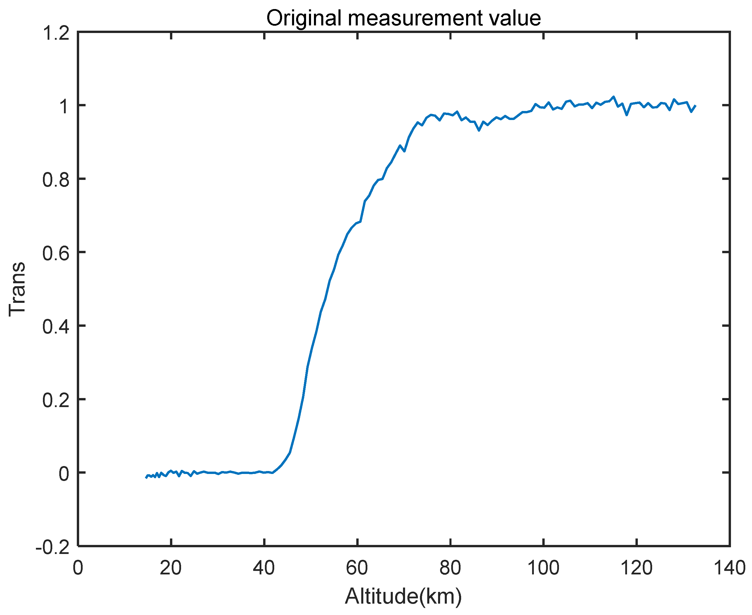
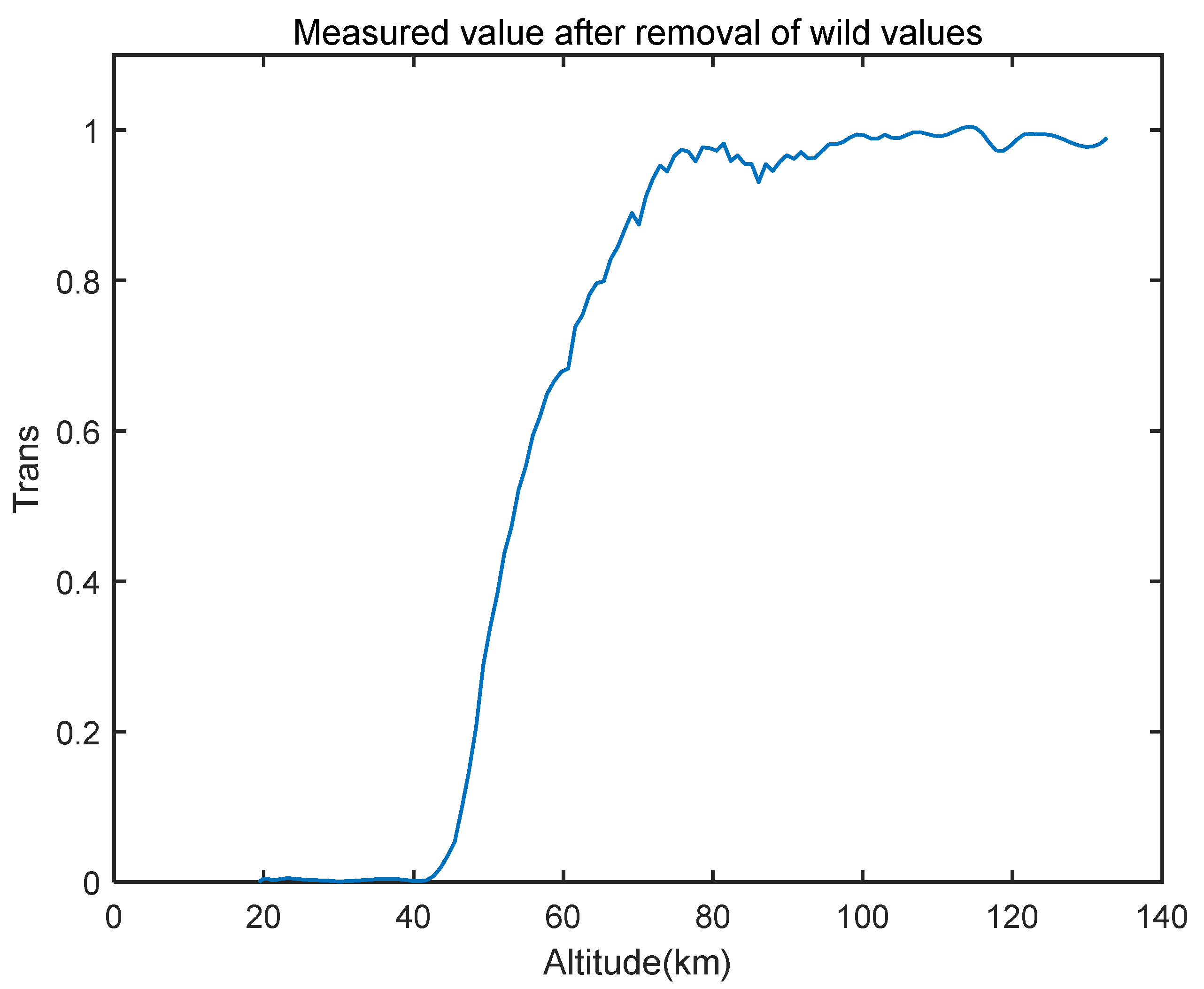
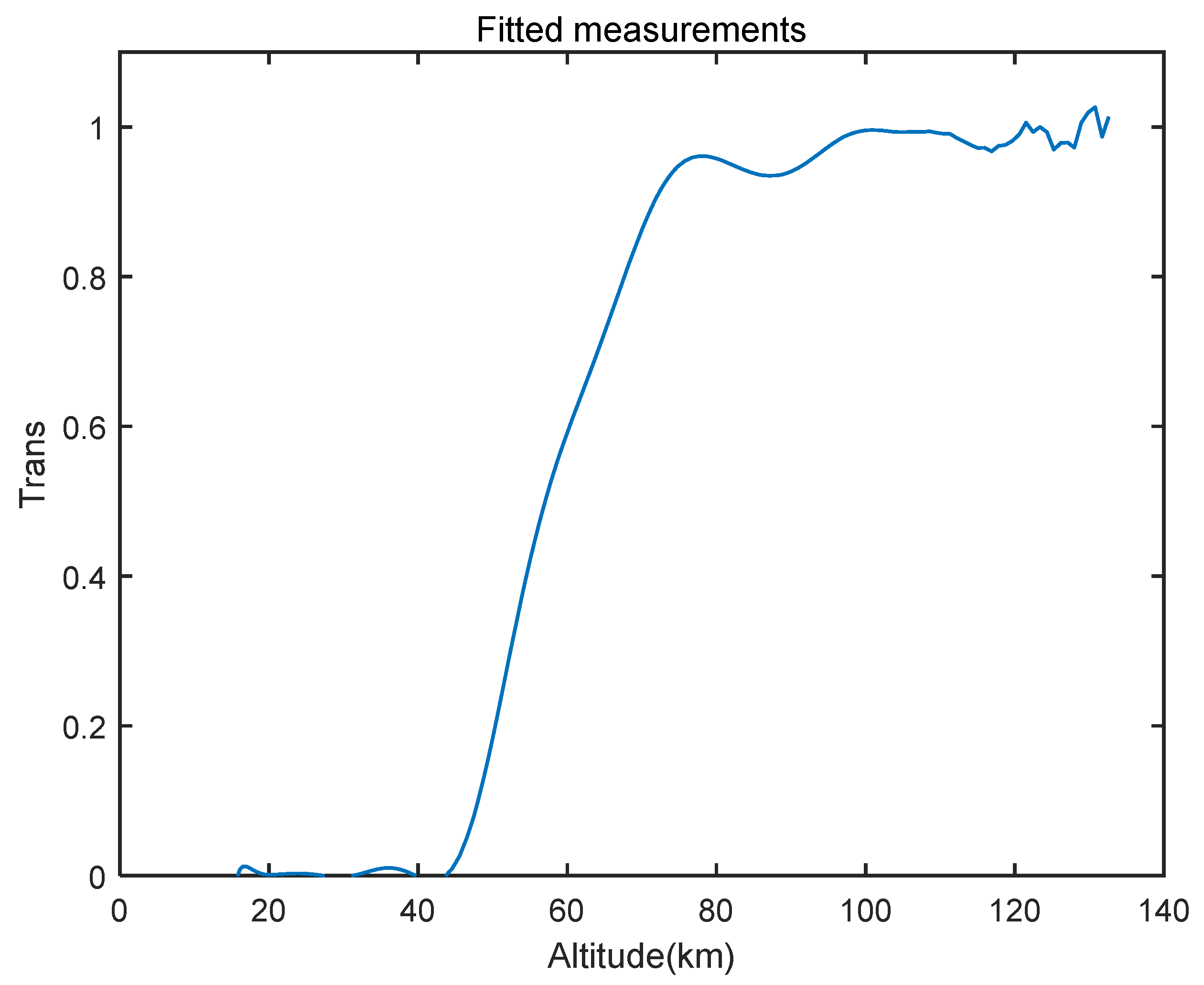
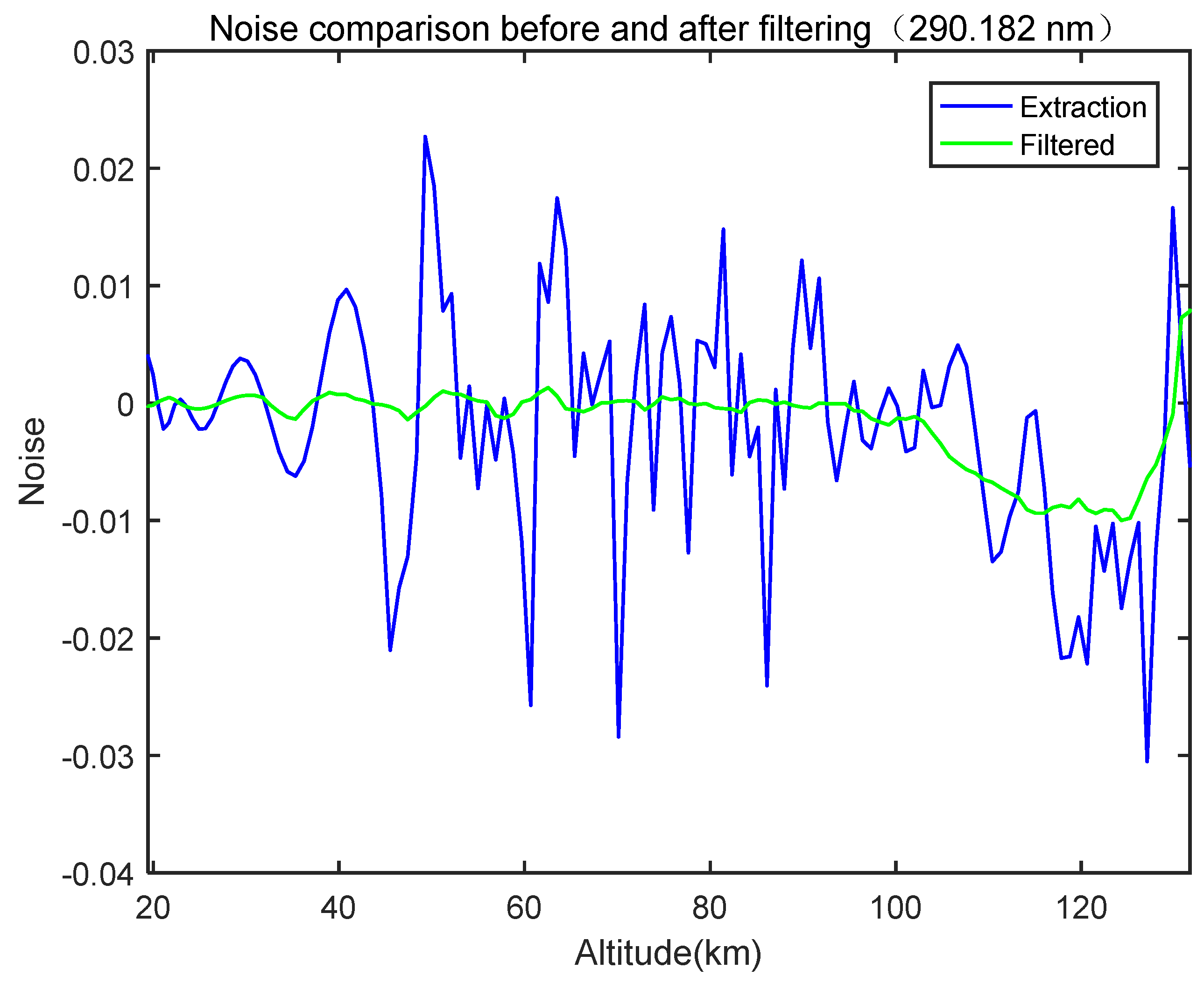
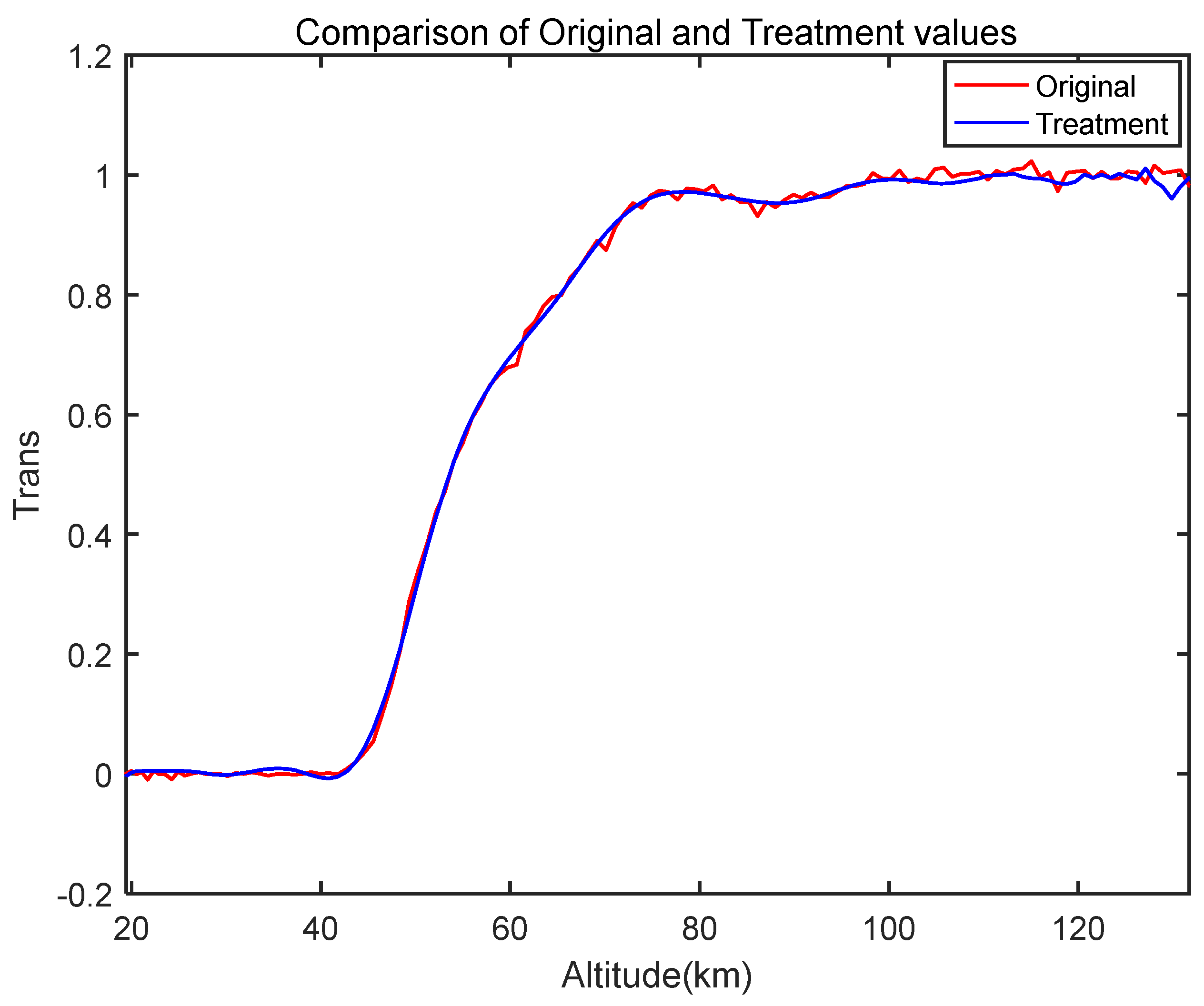
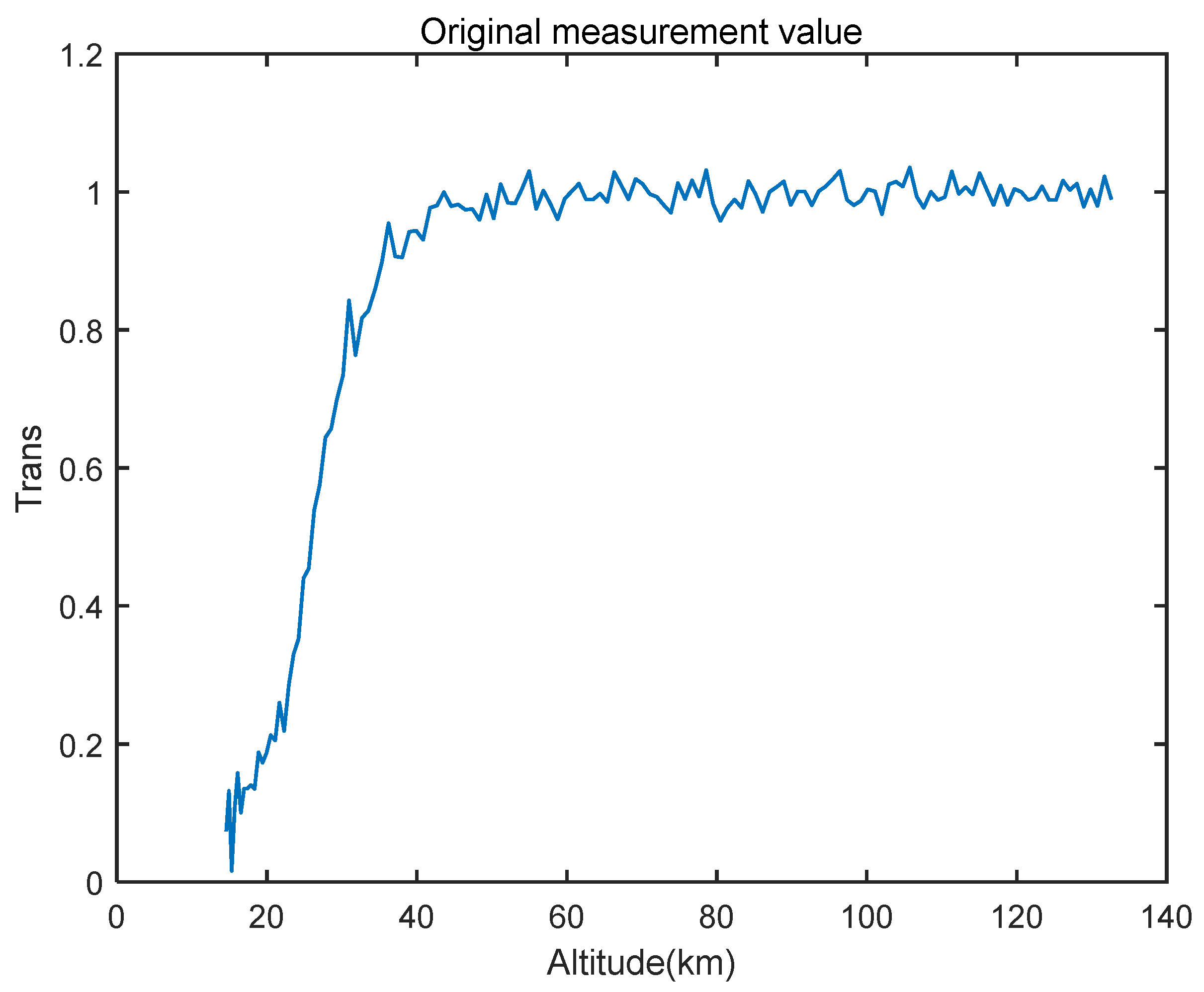
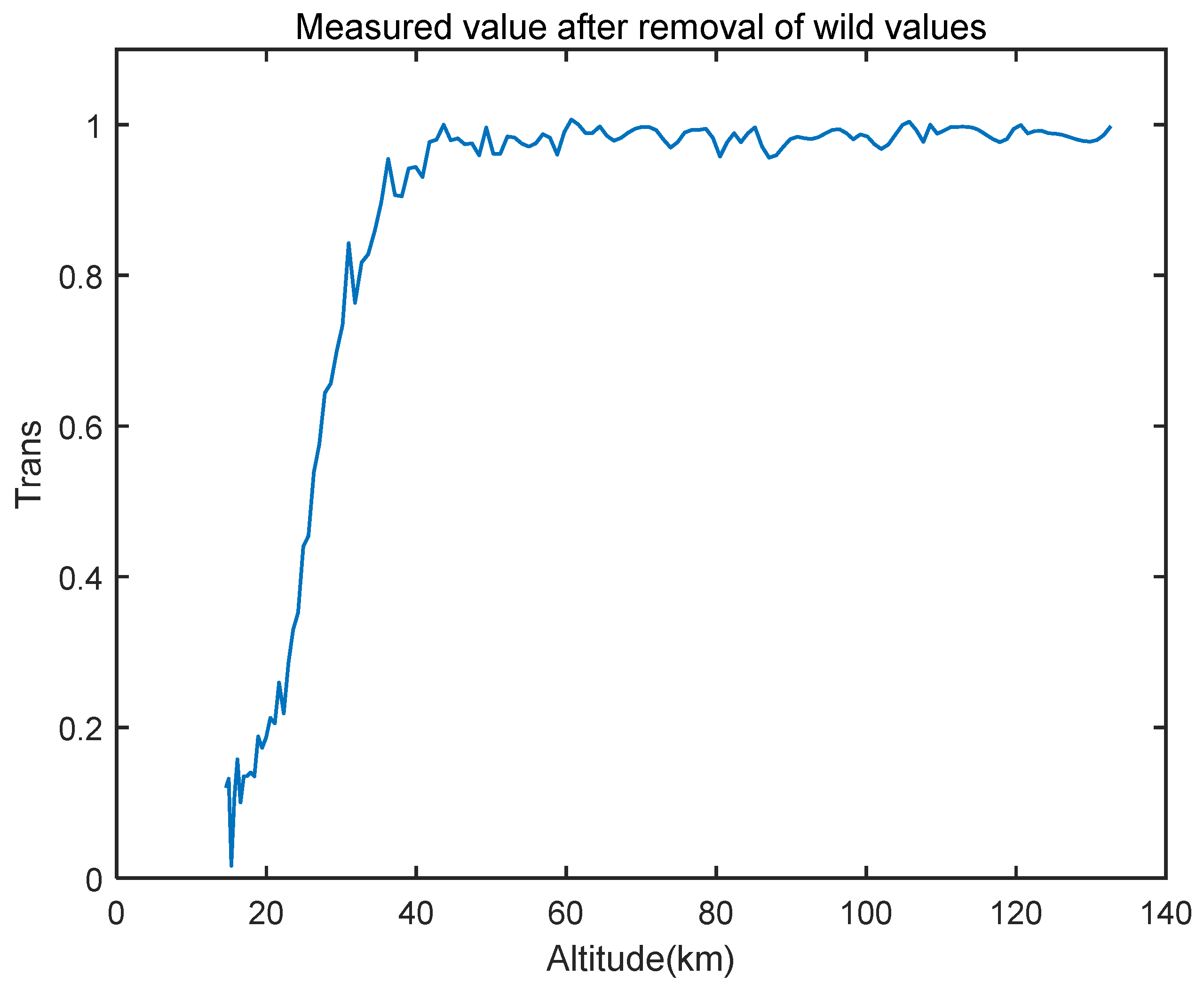
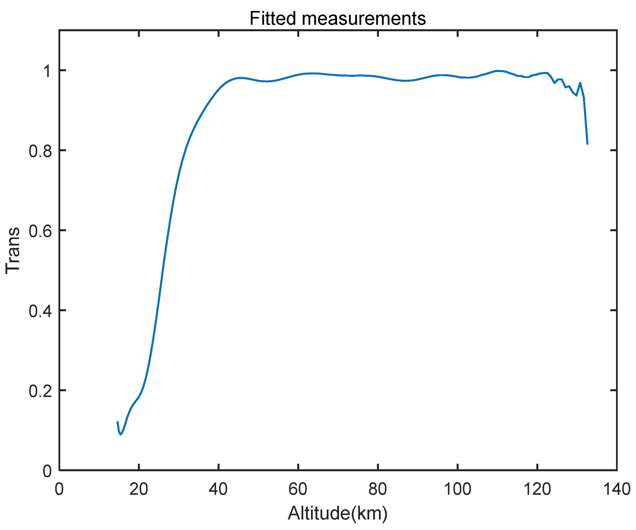
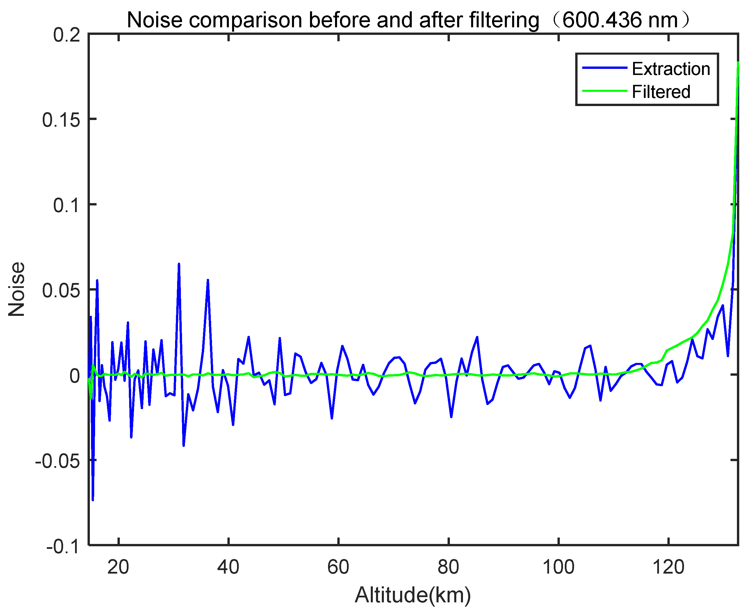
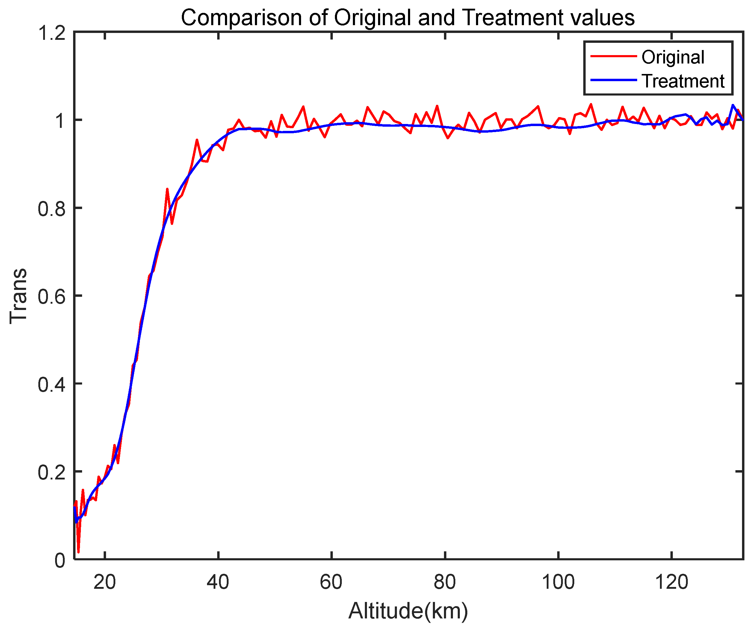
The observed transmittance was obtained directly from the dataset. Prior to inversion, the data were processed as follows: a cubic spline function was used to fit the data and determine the main trend, and the residual data were then Fourier-filtered. Finally, the filtered residual data were combined with a fitted function to obtain the final transmittance curve for data processing. Figure 2, Figure 3, Figure 4, Figure 5 and Figure 6 illustrate the original transmittance at 290.182 nm within the ozone absorption band of 250–300 nm, the transmittance after removing outliers and performing linear interpolation, the fitted transmittance, the extraction and filtering of noise, and the fitting of the observed values.
The following Figure 7, Figure 8, Figure 9, Figure 10 and Figure 11 show the original transmittance, transmittance after removing the wild values and linear interpolation, fitted transmittance, noise extraction and filtering, and observation fitting for the ozone 550–600 nm absorption band at 600.124 nm, respectively.
The noise value determines the quality of the inversion data and, through a noise-filtering process, we controlled the noise value between 0 and 0.01. Therefore, according to the noise value and the results of multi-data processing, we used 50 km as the dividing line, and a short wavelength was used to invert the ozone in the altitude range of 50–130 km. A long wavelength was used to invert the ozone in the altitude range of 15–50 km.
3.3. Comparison of the Results of the Two Inversion Methods
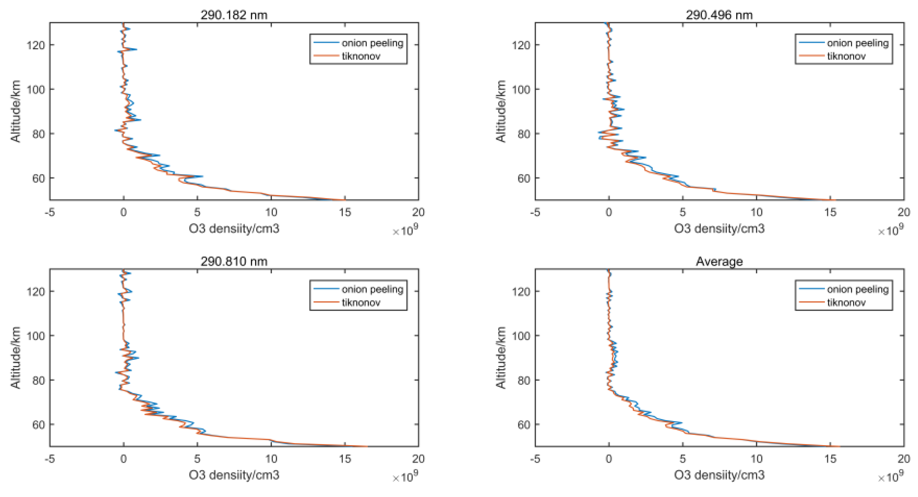
The inversion accuracy for each wavelength varied at different heights. Therefore, it is necessary to select appropriate inversion wavelengths. Ozone exhibits strong absorption bands at 250–300 nm and 550–600 nm. Specifically, there were 162 wavelengths between 250 and 300 nm and 151 wavelengths between 550 and 600 nm. Based on the aforementioned analysis, wavelengths of 290.182 nm, 290.496 nm, and 290.810 nm were chosen to invert the ozone number density at altitudes between 50 and 130 km, while wavelengths of 600.124 nm, 600.436 nm, and 600.747 nm were selected for inversion below 50 km. To accomplish this, a generalised adaptive wild-value rejection algorithm was employed that utilises three times the standard deviation of five consecutive measured data points as the threshold value. This algorithm determined whether the next data point was an outlier or not, and ultimately performed real-time wild-value rejection throughout the process.
The validity of the inversion method was demonstrated using error estimates. Effective cross-sectional and onion-peeling methods were used to invert the same data and calculate the inversion error. The error analysis method involved calculating the single-wavelength inversion results and mean profile relative errors using the GOMOS secondary dataset GOM_NL_2P as the true value.
Comparisons of the inversion results and relative error values for the effective cross-sectional and onion-peeling methods are shown in Figure 12 and Figure 13, respectively.
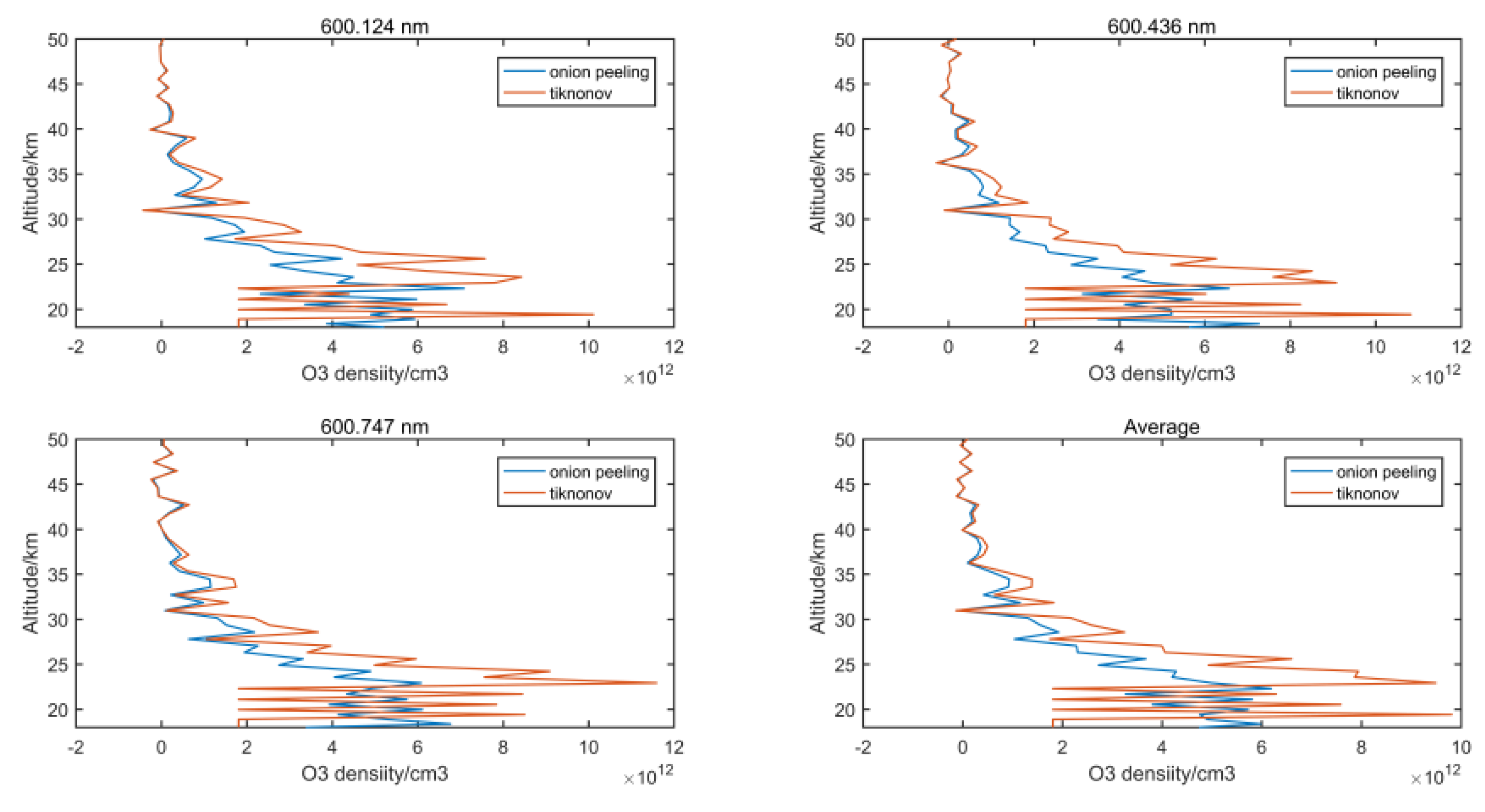
Upon analysing the results presented in the above figures, it is evident that the outcomes obtained from both inversion methods are in strong agreement above an altitude of 30 km. However, at lower altitudes, the deviations between the two methods became more pronounced. Figure 14 and Figure 15 illustrate the error distribution at various altitudes.
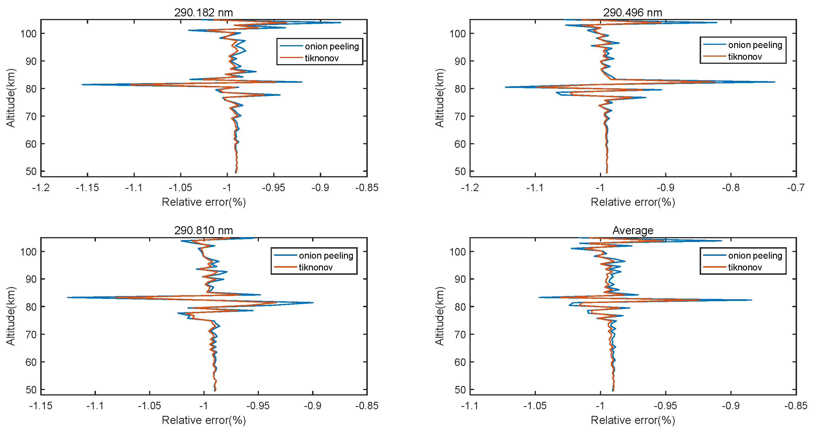
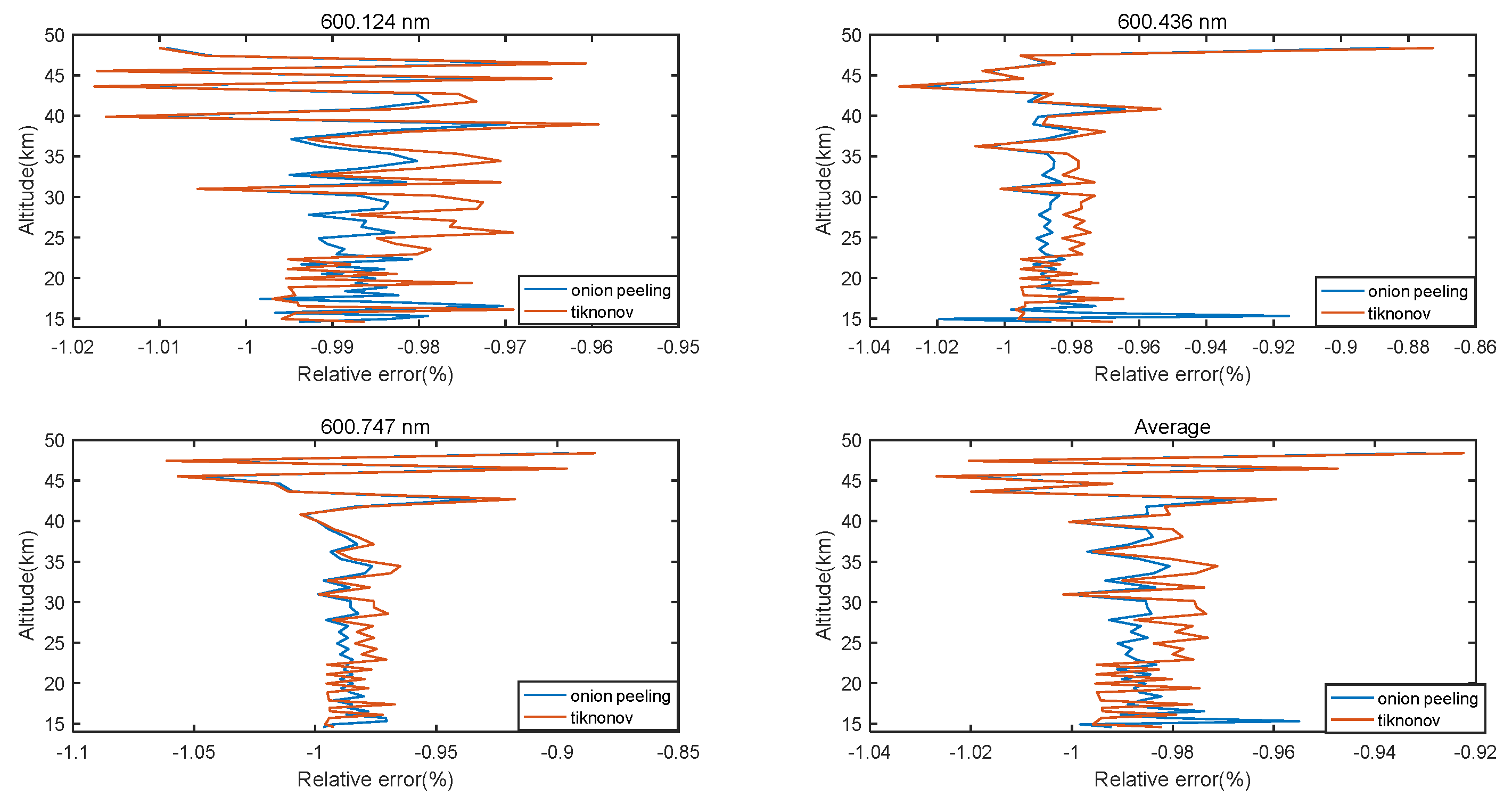
At heights greater than 50 km, the errors of the two inversions were approximately 1%, with a maximum of no more than 1.2%. In general, the errors of the inversions using the effective cross-sectional method were smaller at that height; however, the difference was not significant. Below 50 km, the errors were approximately 1%. In terms of averages, the results of the methodological inversions utilising the effective cross-sectional method were much more accurate, especially at 20–45 km.
3.4. Inversion Results for Other Components
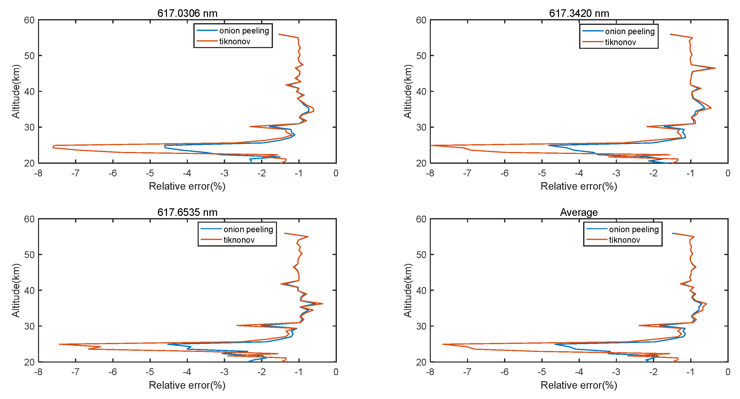
The previous section presented the results of the inversion accuracy. However, further validation is required to compare the results of these two algorithms. and are primarily involved in the catalytic cycling process of . The former is primarily distributed in the stratosphere and has a broad absorption spectrum in the visible region. In contrast, the latter exhibited rapid photodissociation, which occurred only at night, and showed strong absorption peaks at 617 and 655 nm. Therefore, it was unaffected by other components during the inversion process. To illustrate the main idea of this study, we performed the inversion using the same method and observation data from the same time period, and analysed the results. The absorption spectral lines near this peak were observed at 617.0306, 617.3420, and 617.6535 nm. In this study, the error distributions obtained from the two inversion methods were directly compared with the true values. The results are shown in Figure 16.
The results provided the inversion results at the three wavelengths and the error distribution of the mean values. At 30–60 km altitude, the results of the two inversion methods are comparable, with error values between 0 and 2%. However, at approximately 25 km, the inversion accuracy of the onion-peeling method was significantly higher than that of the regularised method, with the former having an error of less than 5% and the latter having an error of up to 8%.
4. Conclusions
Based on the analysis, it can be concluded that:
- The inversion results obtained through the effective cross-sectional method exhibited higher accuracy than the onion-peeling method when the inversion component was ozone, the observed source had an apparent magnitude of 2, the effective temperature exceeded 10,000 K, and the regularisation parameter was set to 1015. This is particularly evident in cases of low-altitude ozone inversion, for which an effective cross-sectional method is recommended. It is crucial to enhance the accuracy of the inversion within an altitude range of 20–45 km, which represents low-altitude regions in the adjacent space.
- Under the same observational conditions used for the inversion of other components, such as nitric oxide, the precision obtained by the onion-peeling method at 25 km was approximately 4% higher than that obtained by the effective cross-sectional method. However, there was little difference between the two methods at other altitudes. This suggests that the parameters and conditions of the effective cross-sectional method are only suitable for ozone inversion, whereas the onion-peeling method is more versatile and applicable to a wider range of components.
Based on these conclusions, we suggest that an effective cross-sectional method is preferred for inverting ozone only if the conditions outlined in this study are satisfied. When inverting other components, it is necessary to modify the regularisation parameter, which depends on the vertical resolution of the different components. However, determining which method exhibits a higher inversion accuracy under different apparent magnitudes and effective temperature conditions requires further investigation. Furthermore, the determination of the regularisation parameter warrants further study to invert the other components using an effective cross-sectional method.
Author Contributions
Conceptualization, M.S. and X.D.; methodology, M.S. and B.X.; software, X.C.; validation, M.S., Q.Z. and X.D.; formal analysis, M.S.; investigation, M.S. and B.X.; resources, Q.Z.; data curation, M.S.; writing—original draft preparation, M.S.; writing—review and editing, X.D. and H.-G.W.; visualization, X.C.; supervision, Q.Z.; project administration, X.C.; funding acquisition, Q.Z. All authors have read and agreed to the published version of the manuscript.
Funding
This research was funded by National Natural Science Foundation of China (Grant No. A072202429 and Grant No. 61971385).
Institutional Review Board Statement
Not applicable.
Informed Consent Statement
Not applicable.
Data Availability Statement
The data presented in this study are available on request from the corresponding author or the official ESA website. The data are publicly available.
Conflicts of Interest
The authors declare no conflict of interest.
References
- Kyrölä, E.; Tamminen, J.; Leppelmeier, G.W.; Sofieva, V.; Hassinen, S.; Bertaux, J.L.; Hauchecorne, A.; Dalaudier, F.; Cot, C.; Korablev, O.; et al. GOMOS on Envisat: An overview. Adv. Space Res. 2004, 33, 1020–1028. [Google Scholar] [CrossRef]
- Kyrölä, E.; Tamminen, J.; Leppelmeier, G.W.; Sofieva, V.; Hassinen, S.; Seppälä, A.; Verronen, P.T.; Bertaux, J.L.; Hauchecorne, A.; Dalaudier, F.; et al. Nighttime ozone profiles in the stratosphere and mesosphere bythe Global Ozone Monitoring by Occultation of Stars on Envisat. J. Geophys. Res. 2006, 111. [Google Scholar] [CrossRef]
- Quémerais, E.; Bertaux, J.L.; Korablev, O.; Dimarellis, E.; Cot, C.; Sandel, B.R.; Fussen, D. Stellar Occultations observed by SPICAM on Mars Express. J. Geophys. Rev. 2006, in press.
- Lebonnois, S.; Quémerais, E.; Montmessin, F.; Lefèvre, F.; Perrier, S.; Bertaux, J.L.; Forget, F. Vertical distribution of ozone on Mars as measured by SPICAM/Mars-Express using stellar occultations. J. Geophys. Rev. 2006, in press.
- Gröller, H.; Montmessin, F.; Yelle, R.V.; Lefèvre, F.; Forget, F.; Schneider, N.M.; Koskinen, T.T.; Deighan, J.; Jain, S.K. MAVEN/IUVS stellar occultation measurements of Mars atmospheric structure and composition. J. Geophys. Res. Planets 2018, 123, 1449–1483. [Google Scholar] [CrossRef]
- Jean-Loup Bertaux, D.; Nevejans, O.; Korablev, E.; Villard, E.; Quémerais, E.; Neefs, F.; Montmessin, F.; Leblanc, J.P.; Dubois, E.; Dimarellis, A.; et al. SPICAV on Venus Express: Three spectrometers to study the global structure and composition of the Venus atmosphere. Planet. Space Sci. 2007, 55, 1673–1700. [Google Scholar] [CrossRef]
- Twomey, S. Introduction to the Mathematics of Inversion in Remote Sensing and Indirect Measurements; Elsevier Science: New York, NY, USA, 1977. [Google Scholar]
- Rodgers, C. Characterization and Error Analysis of Profifiles Retrieved from Remote Sounding Measurements. J. Geophys. Res. 1990, 95, 5587–5595. [Google Scholar] [CrossRef]
- Sun, M.; Dong, X.; Zhu, Q.; Cheng, X.; Wang, H.; Wu, J. Comparison and Analysis of Stellar Occultation Simulation Results and SABER-Satellite-Measured Data in Near Space. Remote Sens. 2022, 14, 5065. [Google Scholar] [CrossRef]
- Zhu, Q.; Sun, M.; Dong, X.; Zhu, P. Design and Simulation of Stellar Occultation Infrared Band Constellation. Remote Sens. 2022, 14, 3327. [Google Scholar] [CrossRef]
- Sun, M.C.; Zhu, Q.L.; Dong, X.; Wu, J.J. Analysis of inversion error characteristics of stellar occultation simulation data. Earth Planet. Phys. 2022, 6, 61–69. [Google Scholar] [CrossRef]
- Kyrölä, E.; Tamminen, J.; Sofieva, V.; Bertaux, J.L.; Hauchecorne, A.; Dalaudier, F.; Fussen, D.; Vanhellemont, F.; Fanton d’Andon, O.; Barrot, G.; et al. Retrieval of atmospheric parameters from GOMOS data. Atmos. Chem. Phys. 2010, 10, 11881–11903. [Google Scholar] [CrossRef]
- Morozov, V.A. Regularization Methods for Ill-Posed Problems; CRC Press: Boca Raton, FL, USA, 1993. [Google Scholar]
- Tikhonov, A.; Arsenin, V. Solutions of Ill-Posed Problems; Wiley: New York, NY, USA, 1977. [Google Scholar]
- Tamminen, J.; Kyrölä, E. Bayesian solution for nonlinear and non-Gaussian inverse problems by Markov chain Monte Carlo method. J. Geophys. Res. 2001, 106, 14377–14390. [Google Scholar] [CrossRef]
- Sofieva, V.F.; Tamminen, J.; Haario, H.; Kyrölä, E.; Lehtinen, M. Ozone profile smoothness as a priori information in the inversion of limb measurements. In Annales Geophysicae; Copernicus Publications: Göttingen, Germany, 2004; Volume 22, pp. 3411–3420. [Google Scholar]
- Honerkamp, J.; Weese, J. Tikhonovs regularization method for ill-posed problems: A comparison of different methods for the determination of the regularization parameter. Contin. Mech. Thermodyn. 1990, 2, 17–30. [Google Scholar] [CrossRef]
- Bertaux, J.L. GOMOS Mission objectives. In Proceedings of the ESAMS99, European Symposium on Atmospheric Measurements from Space, Noordwijk, The Netherlands, 18–22 January 1999; WPP-161. ESA: Noordwijk, The Netherlands, 1999; pp. 79–87. [Google Scholar]
- Bertaux, J.L.; Pellinen, R.; Simon, P.; Chassefière, E.; Dalaudier, F.; Godin, S.; Goutail, F.; Hauchecorne, A.; Le Texier, H.; Mégie, G.; et al. GOMOS, proposal in response to ESA EPOP-1, A.O.1, January, 1988.
- Bertaux, J.L.; Mégie, G.; Widemann, T.; Chassefiere, E.; Pellinen, R.; Kyrölä, E.; Korpela, E.; Simon, P.C. Monitoring of ozone trend by stellar occultations: The Gomos instrument. Adv. Space Res. 1991, 11, 237–242. [Google Scholar] [CrossRef]
- Bertaux, J.L.; Kyrölä, E.; Wehr, T. Stellar Occultation Technique for Atmospheric Ozone Monitoring: GOMOS on Envisat. Earth Obs. Q. 2000, 67, 17–20. [Google Scholar]
- Bertaux, J.L.; Dalaudier, F.; Hauchecorne, A.; et al. Envisat: GOMOS-An instrument for global atmosphere ozone monitoring, edited by: Harris, RA[J]. ESA SP, 1244: 109.
- Bertaux, J.L.; Kyrölä, E.; Fussen, D.; Hauchecorne, A.; Dalaudier, F.; Sofieva, V.; Tamminen, J.; Vanhellemont, F.; Fanton d’Andon, O.; Barrot, G.; et al. Global ozone monitoring by occultation of stars: An overview of GOMOS measurements on ENVISAT. Atmos. Chem. Phys. 2010, 10, 12091–12148. [Google Scholar] [CrossRef]
- Hansen, P.; Jacobsen, B.H.; Mosegaard, K. Methods and Applications of Inversion; Lecture Notes in Earth Science; Springer: Berlin/Heidelberg, Germany, 2000; Volume 92. [Google Scholar]
- Zhang, S.; Wu, X.; Su, M.; Hu, X. Inversion of ozone density by stripping onion of stellar occultation. Spectrosc. Spectr. Anal. 2022, 42, 203–209. (In Chinese) [Google Scholar]
Figure 1.
Schematic diagram of the principle of starlight occultation technology.

Figure 2.
Original transmittance of 290.182 nm.

Figure 3.
Transmittance after removing outliers of 290.182 nm.

Figure 4.
Transmission after polynomial fitting of 290.182 nm.

Figure 5.
Noise value extraction and processing values of 290.182 nm.

Figure 6.
Noise-treated transmittance vs. original value of 290.182 nm.

Figure 7.
Original transmittance of 600.124 nm.

Figure 8.
Transmittance after removing outliers of 600.124 nm.

Figure 9.
Transmission after polynomial fitting of 600.124 nm.

Figure 10.
Noise value extraction and processing values of 600.124 nm.

Figure 11.
Noise-treated transmittance vs. original value of 600.124 nm.

Figure 12.
Comparison of results from two inversion methods at heights above 50 km. It is shown that the inversion results of the two methods are consistent at altitudes above 50 km.
Figure 12.
Comparison of results from two inversion methods at heights above 50 km. It is shown that the inversion results of the two methods are consistent at altitudes above 50 km.

Figure 13.
Comparison of results from two inversion methods at heights below 50 km. It is shown that there is a large difference between the inversion results of the two methods at altitudes below 50 km, especially at lower altitudes.
Figure 13.
Comparison of results from two inversion methods at heights below 50 km. It is shown that there is a large difference between the inversion results of the two methods at altitudes below 50 km, especially at lower altitudes.

Figure 14.
Error distribution of the two inversion methods at heights above 50 km. The figure shows that the errors of both inversion methods are around 1%, with the maximum not exceeding 1.2%, and there is no question of which inversion method is more accurate.
Figure 14.
Error distribution of the two inversion methods at heights above 50 km. The figure shows that the errors of both inversion methods are around 1%, with the maximum not exceeding 1.2%, and there is no question of which inversion method is more accurate.

Figure 15.
Error distribution of the two inversion methods for heights below 50 km. It can be seen that there is a difference in the accuracy of the two inversion methods, especially around 20–45 km, where the error obtained by utilizing the effective cross-sectional area method is smaller, with an overall error of around 1%.

Figure 16.
Error distribution of two inversion methods for nitrogen trioxide. It can be seen that the inversion error obtained using the effective cross-sectional area method reaches 8%, while the inversion error obtained using the peeled onion method is better, with a maximum of 5%.
Figure 16.
Error distribution of two inversion methods for nitrogen trioxide. It can be seen that the inversion error obtained using the effective cross-sectional area method reaches 8%, while the inversion error obtained using the peeled onion method is better, with a maximum of 5%.

Disclaimer/Publisher’s Note: The statements, opinions and data contained in all publications are solely those of the individual author(s) and contributor(s) and not of MDPI and/or the editor(s). MDPI and/or the editor(s) disclaim responsibility for any injury to people or property resulting from any ideas, methods, instructions or products referred to in the content. |
© 2023 by the authors. Licensee MDPI, Basel, Switzerland. This article is an open access article distributed under the terms and conditions of the Creative Commons Attribution (CC BY) license (https://creativecommons.org/licenses/by/4.0/).
Share and Cite
MDPI and ACS Style
Sun, M.; Zhu, Q.; Dong, X.; Xu, B.; Wang, H.-G.; Cheng, X. Comparative Analysis of Starlight Occultation Data Processing. Atmosphere 2023, 14, 1818. https://doi.org/10.3390/atmos14121818
AMA Style
Sun M, Zhu Q, Dong X, Xu B, Wang H-G, Cheng X. Comparative Analysis of Starlight Occultation Data Processing. Atmosphere. 2023; 14(12):1818. https://doi.org/10.3390/atmos14121818
Chicago/Turabian StyleSun, Mingchen, Qinglin Zhu, Xiang Dong, Bin Xu, Hong-Guang Wang, and Xuan Cheng. 2023. "Comparative Analysis of Starlight Occultation Data Processing" Atmosphere 14, no. 12: 1818. https://doi.org/10.3390/atmos14121818
Note that from the first issue of 2016, this journal uses article numbers instead of page numbers. See further details here.