

Oscillations of GW Activities in the MLT Region over Mid-Low-Latitude Area, Kunming Station (25.6° N, 103.8° E)
by
 ,
,
Na Li
1,2,3,
Jinsong Chen
1,2,3,
Jianyuan Wang
1,2,3,*,
Lei Zhao
1,
Zonghua Ding
1,2,3 and
Guojin He
4,* 1
National Key Laboratory of Electromagnetic Environment, China Research Institute of Radiowave Propagation, Qingdao 266107, China
2
Kunming Electro-Magnetic Environment Observation and Research Station, Qujing 655500, China
3
Qujing Electro-Magnetic Environment Observation and Research Station, Qujing 655500, China
4
China Research Institute of Radiowave Propagation, Qingdao 266107, China
*
Authors to whom correspondence should be addressed.
Atmosphere 2023, 14(12), 1810; https://doi.org/10.3390/atmos14121810
Submission received: 14 October 2023
/
Revised: 8 November 2023
/
Accepted: 5 December 2023
/
Published: 11 December 2023
(This article belongs to the Special Issue Intelligent Modeling of the Ionosphere and Troposphere for Radio Application)
Abstract
:Gravity wave (GW) activities play a prominent role in the complex coupling process of wave–wave and wave–background circulation around mid-low-latitude and equatorial areas. The wavelengths are wide, from about 10 m to 100 km, with a period from minutes to hours. However, the oscillations of GW activities are apparently different between the period bands of 0.1 to 1 h (HF) and 1 to 5 h (LF). To further understand the characteristics of GW activities, the neutral winds during 2008–2009 with a resolution of 3 min obtained from a medium-frequency (MF) radar in Kunming (25.6° N, 103.8° E) were analyzed. Using two numerical filters, the HF and LF GWs were estimated. Interestingly, the power spectral density grows larger as the frequency increases. It linearly falls with decreasing frequency when the period is less than 2 h. The seasonal variations in both HF and LF GWs are strongly demonstrated in August–September, November, and February–March with maximum meridional variances of 1100 m2 s−2 and 500 m2 s−2 and maximum zonal variances of 800 m2 s−2 and 350 m2 s−2 in, respectively. The turbulent velocity was also calculated and shows similar oscillations with GW activities. Furthermore, the GW propagation direction exhibits strong seasonal variations, which may be dependent on the location of the motivating source and background wind.
1. Introduction
Atmospheric GWs (GWs) usually originate in the lower atmosphere and propagate upward to the middle and upper atmosphere, and they play an essential role in the coupling process between the lower and upper atmosphere [1]. The periods of GWs change from several minutes to hours. Their horizontal wavelengths may vary from 10 m to more than 100 km [2]. Their amplitude enlarges dramatically with a quick reduction in atmosphere pressure when they propagate upward. When GWs are under critical status, they deposit their energy and transfer their momentum to the mean flow [3,4]. The main sources of GWs have been considered as including orography, convection [5,6], frontal systems [4], wind shear [7], volcanic eruptions [8,9,10,11], and earthquakes [12]. As reported by Plougonven et al. (2020), GWs have been taken as a main coupling mechanism linking different atmosphere regions because GWs continuously transport energy and momentum from the lower atmosphere to higher altitudes [13].
During the past few decades, several studies have been devoted to understanding the behaviors of GWs based on different instruments. Franco-Diaz et al. (2023) utilized horizontal brightness temperature data from the AIRS and lidar to highlight sporadic peaks in GW activity due to tropospheric deep convective events. They found that sporadic peaks in GW activity in summer greatly exceeded those in winter [6]. During the summer–winter transition, the GWs with periods of 3–5 h dominate the mesopause region above the Northern Hemisphere mid-latitudes [14]. Meanwhile, AIRS and MLS satellite data also show a strong atmospheric GW in the stratosphere about 8.5 h after the eruption of the Hunga Tonga–Hunga Ha’apai volcano [8]. Li, J and Lu. X (2022) analyzed 17-year SABER-observed GW temperature variances [15]. They found that the Madden–Julian Oscillation (MJO) could significantly affect GWs over the middle atmosphere (30–100 km) in the tropics and extra-tropics (45° S to 45° N) for northern winter [16]. Certainly, the temperature data from daylight-capable Rayleigh–Mie–Raman lidar measurements also prove that the 24 h wave occurs between 40 and 60 km and vanishes due to an enhancement of gravity waves with periods of 4–8 h [17]. As a conventional ground-based instrument, meteor radar or medium radar is used to observe neutral winds, which are always employed to investigate the behaviors of high-frequency GWs. Pramitha et al. (2020) used meteor radar observations for the first time to investigate the GW source spectrum [18]. Matsumoto et al. (2016) found significant semiannual and annual oscillations in seasonal variations in the momentum flux based on data from two nearly identical meteor radars at Koto Tabang (0.2° S, 100.32° E), West Sumatra, and Biak (1.17° S, 136.1° E), West Papua [19]. Based on two meteor radars at Mohe and Wuhan, Wu et al. (2022) presented an anticorrelated pattern of meridional momentum flux of GWs to the meridional wind pattern at Mohe due to the wind filtering of GWs [20]. Moreover, the correlation of meridional momentum flux with the background meridional wind was not seen at Wuhan. Manson et al. [21] investigated the wind data for the years 1992 and 1993 obtained from an MF radar (52° N, 107° W) at Saskatoon. They found that a 6 h modulation was presented clearly in the momentum flux of GWs when the propagation directions of the momentum flux of GWs were isotropic.
Indeed, as much as 70% of the momentum transported into the MLT region is due to short-period (<1 h) GWs penetrating the MLT region from below [16]. The retrieval of short-period (<1 h) GWs strongly requires high detection capabilities of instruments with a temporal resolution far less than 1 h. MF radar can detect the neutral wind and electron density within the height range of 60–100 km with temporal and vertical resolutions of 2 km and 3 min, respectively. Gavrilov et al. (2002) analyzed wind variances with period bands of 0.1 to 1 h and 1 to 5 h based on data from an MF radar on the island of Kauai, Hawaii (22° N, 160° W) [22]. They found that the mean zonal wind has mainly an annual variation below an altitude of 83 km and a semiannual variation above. The maximum intensity of GWs occurred at the solstices below 83 but shifted to the equinoxes at higher altitudes.
The maximum electron density in the ionosphere F region is usually located on either side of the magnetic equator in the daytime, which is named the Equatorial Ionospheric Anomaly (EIA) crest [23]. The EIA phenomenon is significant from afternoon to sunset due to the dominating atmospheric dynamo effect in the daytime [24]. The key mechanism has been considered to be the tidal winds modulating the dynamo effect in the E layer and leading to the upward EXB drift generated by the eastward electric field, further forming the EIA phenomenon [25]. Subsequently, the atmospheric coupling process and mechanism have sprung up [26,27,28,29,30,31]. However, many questions remain to be answered.
Kunming station is located at a geographic latitude of 25.6° N corresponding to the geomagnetic latitude of about 18.8° N, which lies around the northern hump zone of the Equatorial Ionospheric Anomaly crest [32,33]. Meanwhile, Kunming station is located on the Yunnan–Guizhou Plateau, which greatly influences the atmosphere coupling process due to its effect on background circulation. Since 2008, systematic measurements of wind velocity at altitudes of 60–100 km have been made using a medium-frequency (MF) radar and a meteor radar on the same observation platform. These radars have been used for investigations of variations in waves (e.g., tides, planetary waves), responses to events, and lower ionosphere [32,33,34,35]. The prominent advantage of MF radar is its temporal resolution of 3 min compared to the 1 h of meteor radar.
This work mainly addresses the oscillations of high (0.1–1 h) and low (1–5 h) frequency GWs obtained from Kunming MF radar. The data analysis methods are described in Section 2. The month oscillations of GWs in 2008–2009 are displayed in Section 3. Some of the observed peculiarities of GW variations at Kunming are also discussed in Section 4. At last, in Section 5, the conclusion is given.
2. Data and Processing Method
2.1. Kunming MF Radar
The Kunming MF radar was established in 2008 and is running every day. Its detecting height range is 60–100 km with vertical and temporal resolutions of 2 km and 3 min. Its working frequency is 2.138 MHz, with a transmitter peak power of 64 kW. Kunming MF radar works the O-mode during the day and the E-mode at night and has a unique antenna configuration of four sets of crossed dipoles at a height of 30 m to form an equilateral triangle with sides of 170 m. The four cross dipoles are assigned for both transmission and reception. The main specifications of the Kunming MF radar are presented in Table 1. Since then, continuous observation of winds in the MLT has been underway and allows us to study atmospheric oscillations in the low-latitude MLT region and wave–wave nonlinear interaction. More details on this MF radar description can be seen elsewhere [33]. For MF radar, the standard full correlation (FCA) method [36] is used to obtain the wind data from the raw observation. The details about the basic specifications of FCA wind measurement are shown in Table 2.
2.2. Datasets and Analysis Method
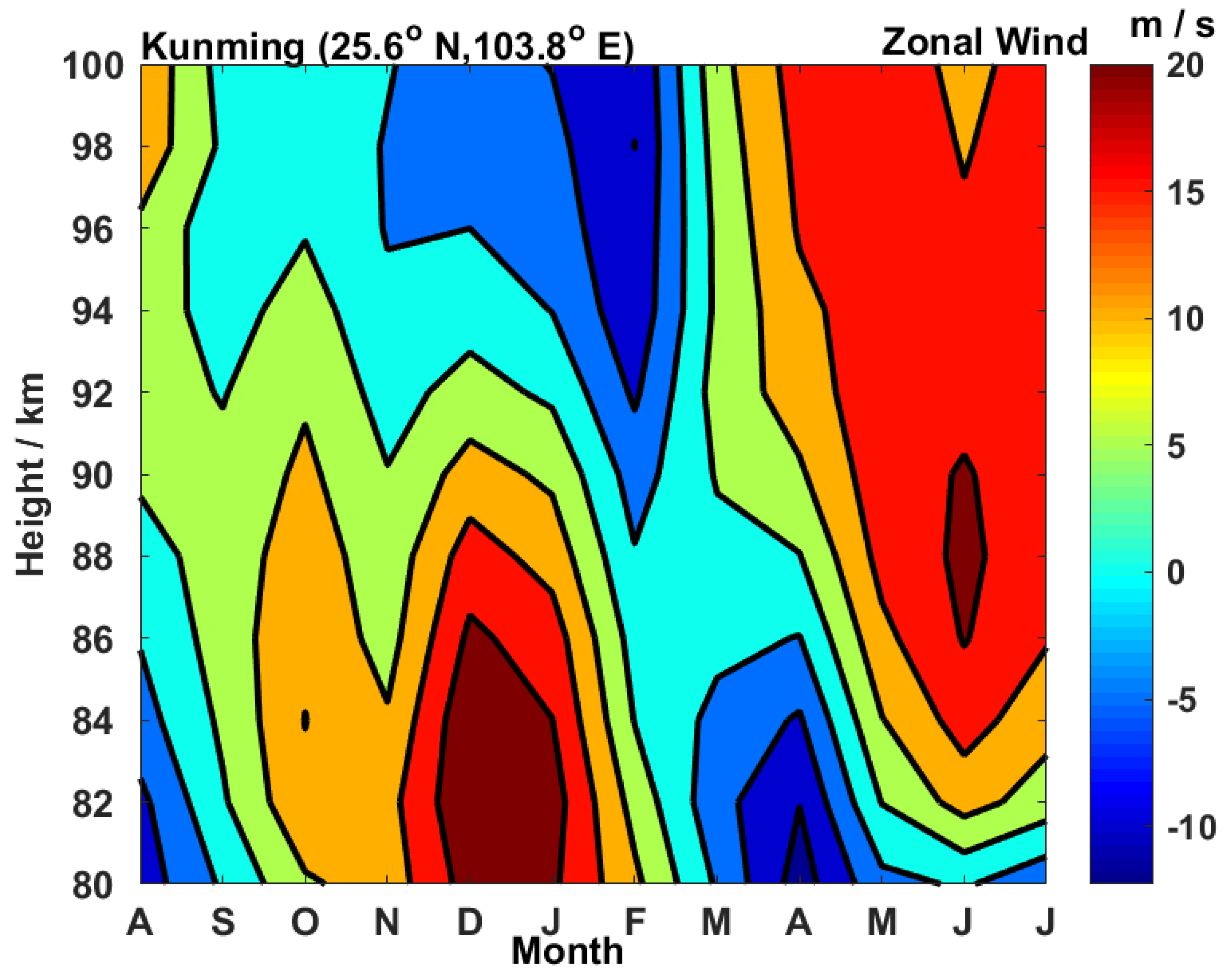
The wind data from August 2008–July 2009 were utilized in this study, shown in Figure 1 for just the zonal wind. As known from Figure 1, the monthly averaged zonal wind prevails eastward from November to February below 90 km and from May to June above 82 km; however, it is westward from November to March above 92 km and from March to April below 84 km. In other words, the semiannual variation is significant. Moreover, the wind shear occurs around 90 km with lively GW activities. In past, the validity of MF radar measurement has been discussed in the reference Li et al. (2015) [35]. In that work, the comparison of wind data and HWM07 shows that the error range was within the acceptable scale, although there was some visible difference between them.
The Kunming MF radar data have some gaps because of instrumental failure or other unpredictable reasons. In particular, the percentage of missing data can be substantial, which may make it difficult to obtain reliable calculations in this work. To obtain the main GW parameter, the bandpass filter was employed at every height and every day in this study due to its advantage of the lesser dependence of the filtered values on the gap in the experimental data. At each height vs. day bin between 80 and 100 km, we first calculate the averaged values and standard deviations within two windows of 0.1–1 h and 1–5 h to obtain hourly mean values of the zonal and meridional wind velocity components. Then, the hourly averages were subtracted from observations to obtain the corresponding hourly variances. Indeed, the variances providing important information about wind perturbations with a timescale of 0.1 to 1 h were designated as “high-frequency” (HF) variances, and those with a timescale of 1 to 5 h were taken as “low-frequency” (LF) variances. Then, we calculated the differences between consecutive hourly velocity values, which meant a numerical bandpass filter passing harmonics with the periods of 0.1 to 1 h and 1 to 5 h. One point should be noted, that the differences between hourly velocity values at given altitudes must be considered when we calculate the LF variances, and there is a transmission maximum at a period of 2 h.
As described by Gavrilov et al. (2003), the number of valid velocity measurements () during each hour must be taken into account in the process of calculating monthly averages because the data confidence is different at every altitude within the range of 70–90 km [22].
where denotes the hourly mean wind velocities or HF and LF wind variances in a particular month.
During the daytime, the pulse repeat frequency (PRF) of MF radar is 80 Hz with 32-point coherent integration, while at night, the PRF is reduced to 40 Hz with 16-point coherent integration. So, wind measurement via MF radar is usually impossible below 80 km at night due to the lack of ionization; in other words, at lower altitudes, the percentage of missing data can be substantial. In this study, we rejected mean wind and HF variance estimates with less than 8 points in a 1 h interval. With such a criterion, the total relative number of data gaps and rejected data points is 70–90% near an altitude of 70 km. At higher altitudes, the number of data gaps decreases and has a minimum of 10–40% for different months at altitudes 85–88 km. Therefore, the proportion of monthly data gaps is 10–60% at altitudes of 80–90 km. In this study, we used the data covering the altitude region 80–100 km and divided it into two parts at 90 km.
3. Results
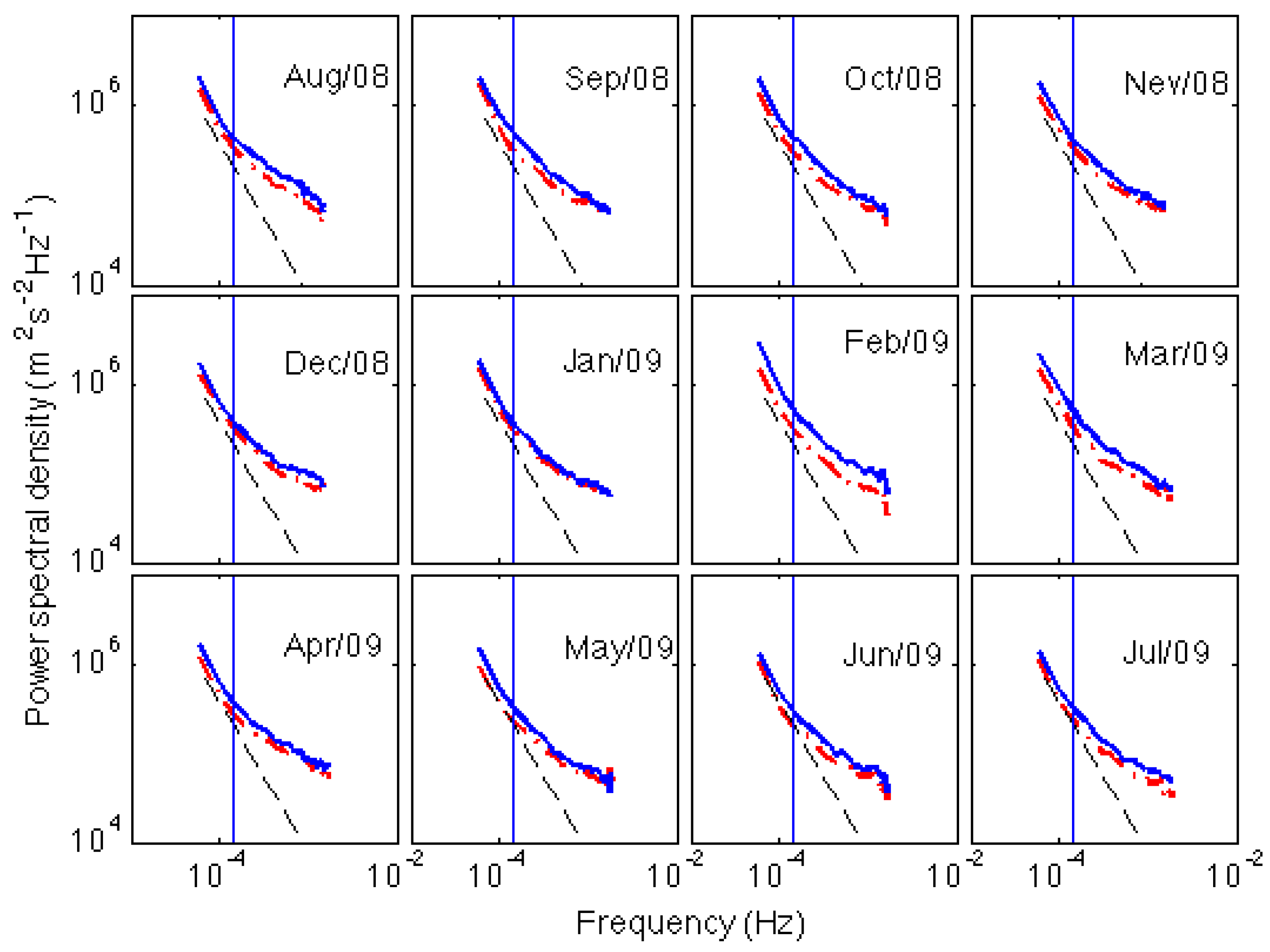
Figure 2 presents the monthly frequency spectra for zonal winds (red dotted line) and meridional winds (blue solid line) from the Kunming MF radar from August 2008 to July 2009. The dashed straight line has a slope of −5/3, and the vertical straight line indicates a period of 2 h. The power spectral density decreases near-linearly as the frequency in the zonal and meridional directions decreases when the period is shorter than 2 h. Moreover, the power spectral density for two directions is above the slope of −5/3 from August 2008 to April 2009, while the zonal spectral density matches the slope of −5/3 very well from May to July 2009. When the period is longer than 2 h, the descending gradient is smaller and smaller in all months as the frequency decreases. In addition, the power spectral density in the zonal direction is close to that in the meridional direction with a threshold of around 0.5 × 10⁵, especially in January, besides that in February and March 2009. In February and March 2009, the spectral density behaviors were significantly greater in the meridional direction, which is also slightly seen in September–October. The result shown in Figure 2 reveals that the momentum and energy mainly concentrate the waves with high frequency.
The power spectral density shown in Figure 2 reveals motions at different frequencies with distinct features. Small-scale GWs with a period of <1 h are responsible for as much as 70% of the wave-induced transport that occurs in the MLT region [16]. To investigate the seasonal variability of wave fluxes, the wind variances in the zonal and meridional components are displayed with the period range of 0.1 to 1 h and 1 to 5 h, as shown in Figure 3, Figure 4, Figure 5 and Figure 6.
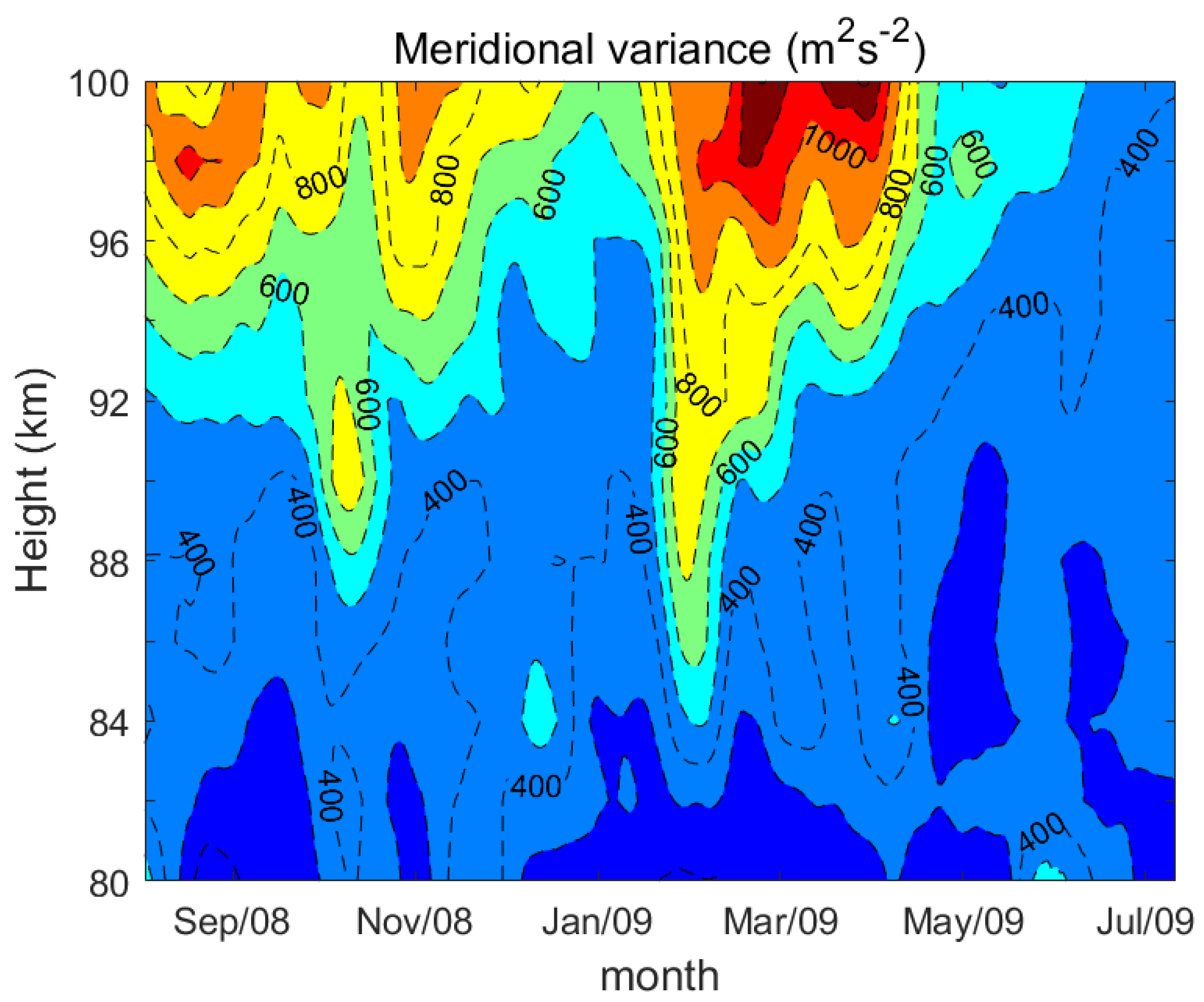
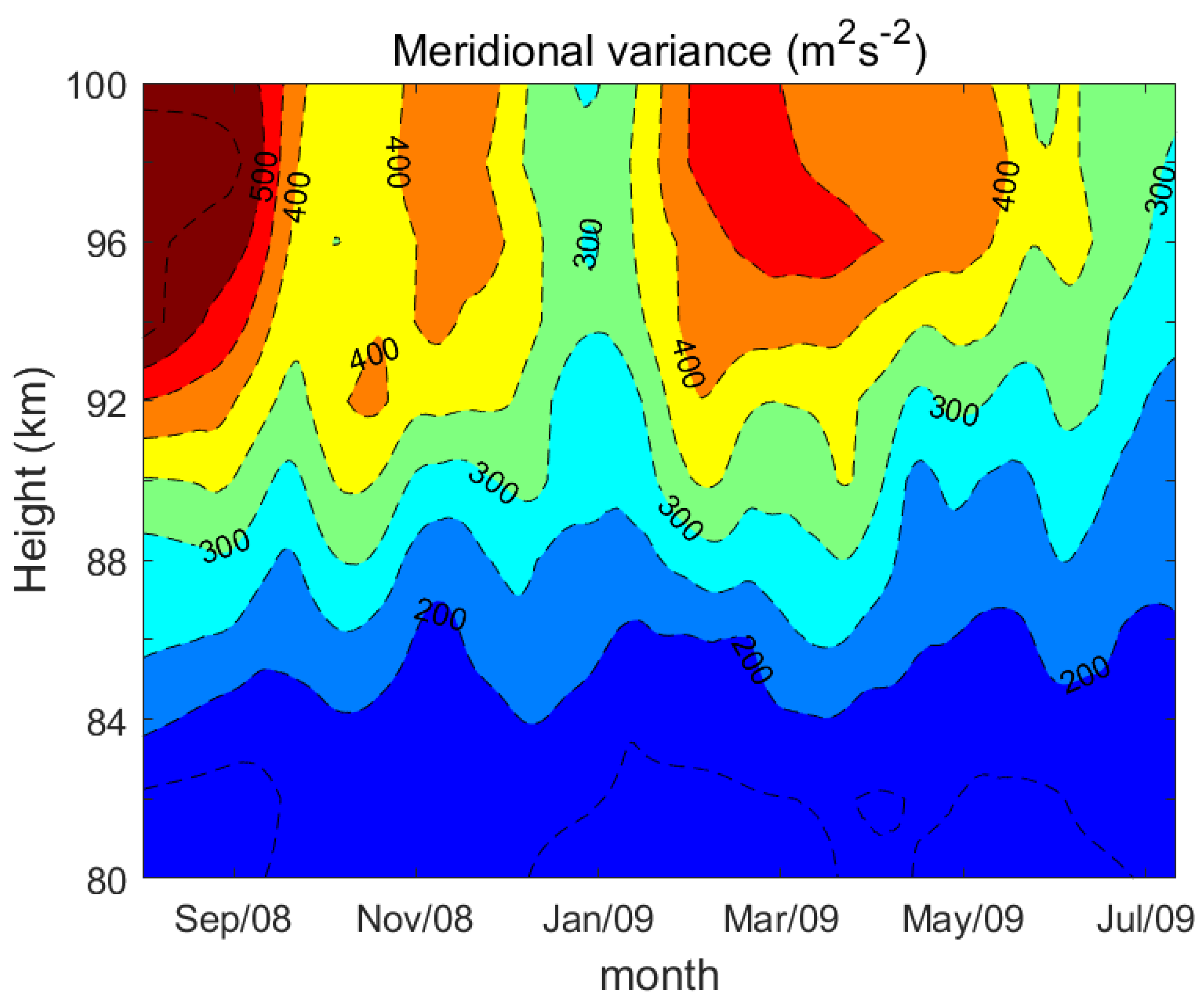
As can be seen from Figure 3, the meridional GW variance with the period of <1 h grows upward with increasing altitude in all months. For example, below 98 km, the level of meridional GW variance mainly stays around 400 m2 s−2 and increases up to 1200 m2 s−2 at 100 km in March 2009. The changes in meridional GW variance have no clear relation with altitude in June-July 2009 and are at peace under a lower level. An important point is that significant semiannual variability is shown below 90 km, with peaks of 800 m2 s−2 occurring in October 2008 and February 2009, and prominent seasonal variability is clearer above 90 km. Taking the altitude of 98 km as an example, the meridional GW variance reaches six peaks in September, October, and November 2008 and February, March, and April 2009 with values of 1000 m2 s−2, 800 m2 s−2, and 1000 m2 s−2 and 1000 m2 s−2, 1200 m2 s−2, and 1000 m2 s−2, respectively. The results from Figure 3 illustrate that the GW momentum in the meridional direction plays a dominating role in spring and autumn at higher altitudes over Kunming.
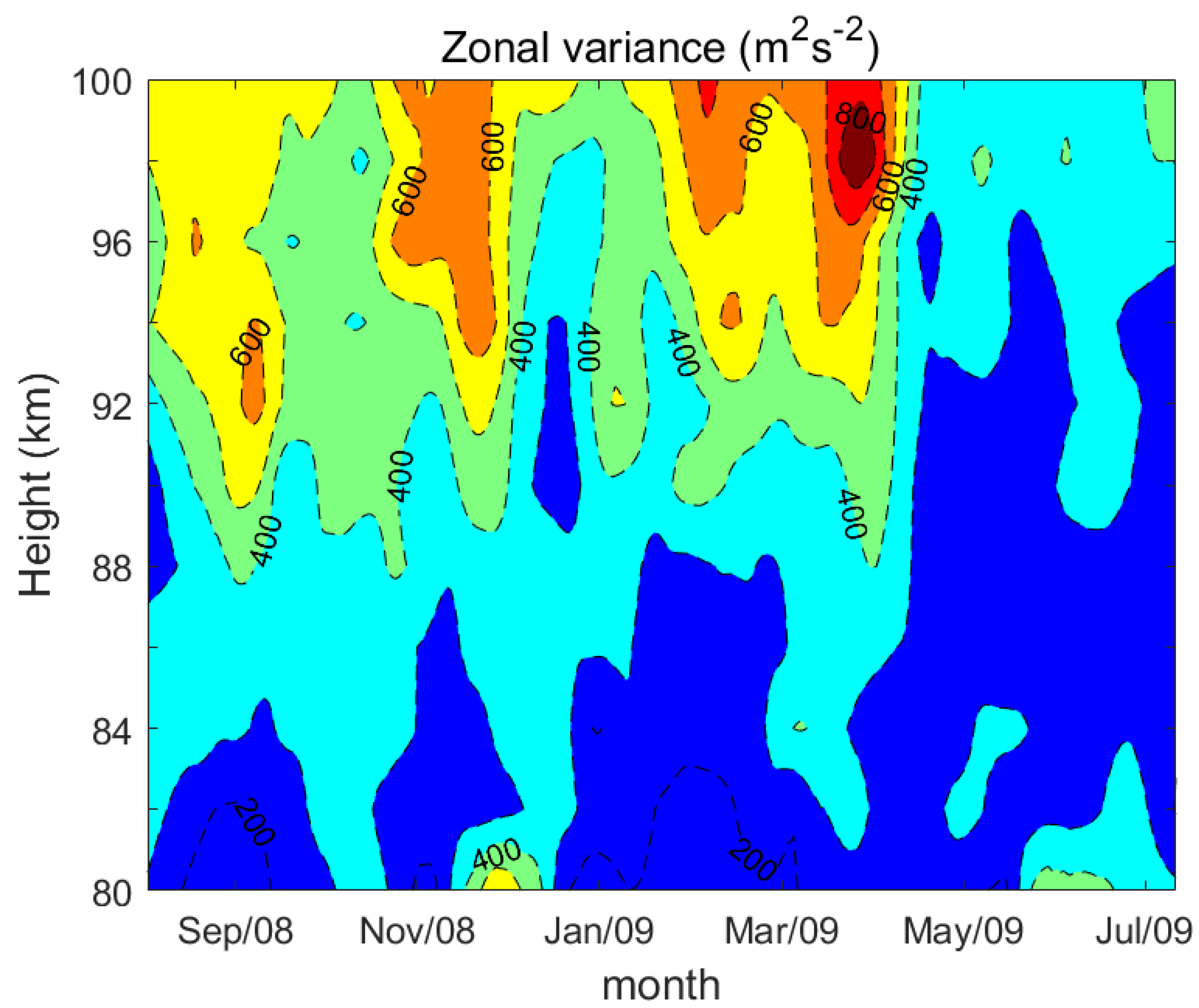
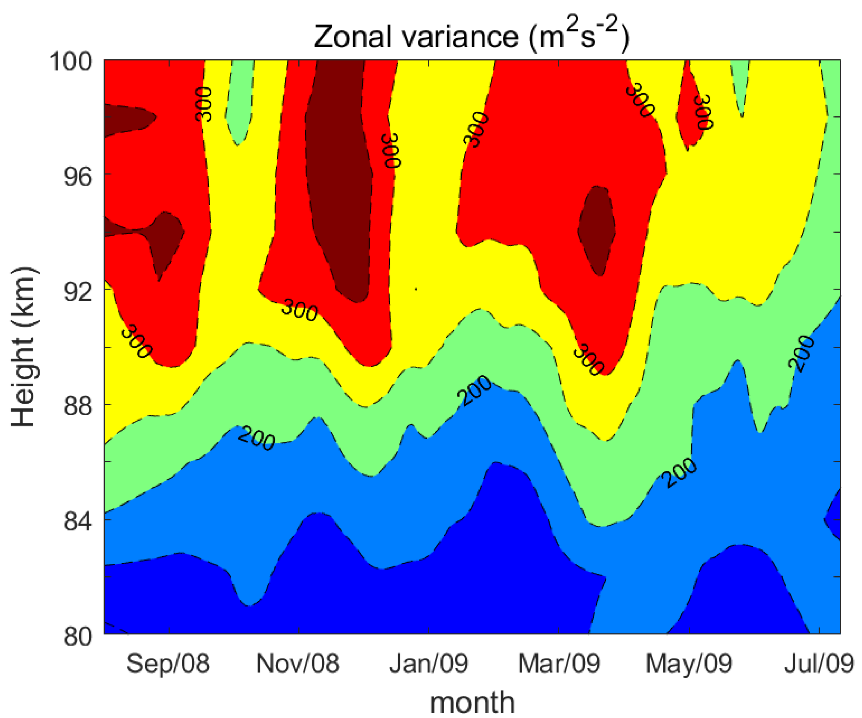
Figure 4 shows the changes in zonal GW variance with the period of <1 h from August 2008 to July 2009 with altitude. Similar to that in Figure 3, the contours are also plotted at 200 m2 s−2 intervals. However, seasonal variability dominates all altitudes and months. Below 88 km, the zonal GW variance shows several peaks in August, October, and December 2008 and March, May, and June 2009 with a maximum of 500 m2 s−2. Above 88 km, the peaks of zonal GW variance appear in September, October, December, January, February, and April with a maximum of 800 m2 s−2. For all altitudes, no semiannual variability can be found from August 2008 to July 2009. The peak of zonal GW variance is smaller in comparison to that of meridional GW variance. Two unexpected enhancements can also be found in December and June at 80 km, which may be affected by other events investigated in future work. It is easy to know that the GW variances are stronger above 90 km and focus on autumn and spring. The seasonal variability should be the most important feature for the HF GW variance.
Figure 5 and Figure 6 show altitude–seasonal variations in LF GW variances; the contours are plotted at 50 m2 s−2 intervals. One can see that the meridional GW variance is enhanced (shown in Figure 5) strictly with increasing height in every month besides January and July. The magnitude of meridional GW variance is as low as 200 m2 s−2 below 84 km in all months. When the height is up to and above 84 km, the seasonal variability becomes more significant with increasing height. The peaks repeat every two months at the altitude range of 84 km–92 km. Meanwhile, the meridional LF GW variance has regular changes with a period of around 90 days, which may have some relation to the MJO phenomenon [15]. In the year of August 2008 to July 2009, the maximum occurred in August 2008 with a value of 500 m2 s−2. Differently from the HF GW variance, the momentum and energy primarily congregate in August-September and spring above 92 km. Similar to Figure 5, the zonal GW variance behaves strongly toward seasonal variation. The seasonal peaks always occur in September, December, and March above 88 km and in October, January, and April below 88 km. The peak value of 400 m2 s−2 can be found in September, December, and March, respectively, which is slightly smaller than that in the meridional direction.
4. Discussion
As seen from Figure 3, Figure 4, Figure 5 and Figure 6, the enhancement of the GW variance at higher frequencies can be considered to be possibly caused by contamination from the horizontal differences of the vertical wind in the radar sampling volume [37]. The magnitude of GW variance with a period of 1–5 h is less than that with a period of <1 h, which is probably because the vertical wavelengths of observed GWs are generally smaller for the waves with longer periods shown by Manson and Meek [38].
Extensive studies on GWs in the middle atmosphere have received attention over the past several dozen years based on a variety of techniques [6,20,22,39,40,41] and reports of seasonal variations in GWs in some locations. Particularly, one noted feature of GW climatologies common in these observations is pointed out, the semiannual variation in the GW activity at mesospheric heights, with maximum activity occurring during the winter and summer months. In this study, the semiannual variation in the GW activity is highlighted in the meridional variance with a period of <1 h below 90 km shown in Figure 3, with the maximum occurring in October and February. However, the seasonal variability is more significant in the zonal variance with periods of 0.1–1 h and 1–5 h and in the meridional variance with a period of 1–5 h.
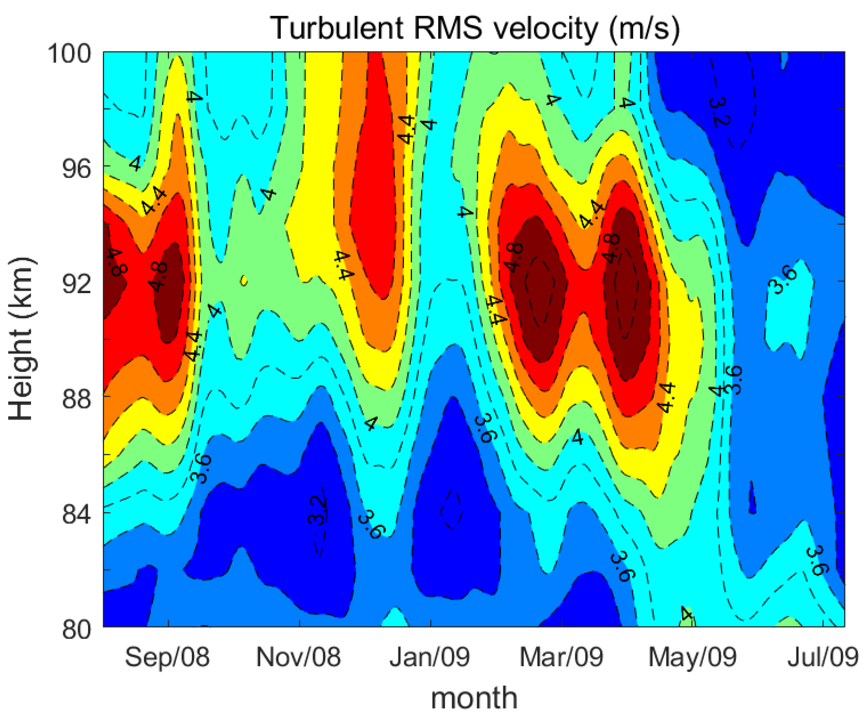
The amplitudes of upward propagating GWs will grow with altitude due to the decrease in density. When the large value increases to the dynamic instability threshold, the wave breaks and yields intense turbulence, leading to the dissipation of energy and momentum, as well as the diffusion and mixing of constituents. One of the most essential turbulence parameters is the dissipation rate of turbulent kinetic energy ε. Additionally, the turbulent kinetic energy is expressed as , with . Here, the turbulence variance derived from the Kunming MF radar is given in Figure 7. Interestingly, the turbulent velocity is especially strong within the height range of 86 km–98 km, with the maxima of 50 m/s occurring around 92 km. In conclusion, the durations when the turbulent velocity continues strongly are in August-September, December, and February-April, respectively. These durations are consistent with the time when the zonal or meridional variances are strong, shown in Figure 3, Figure 4, Figure 5 and Figure 6. In other words, the seasonal variation in GW activity at Kunming is indeed a very remarkable feature.
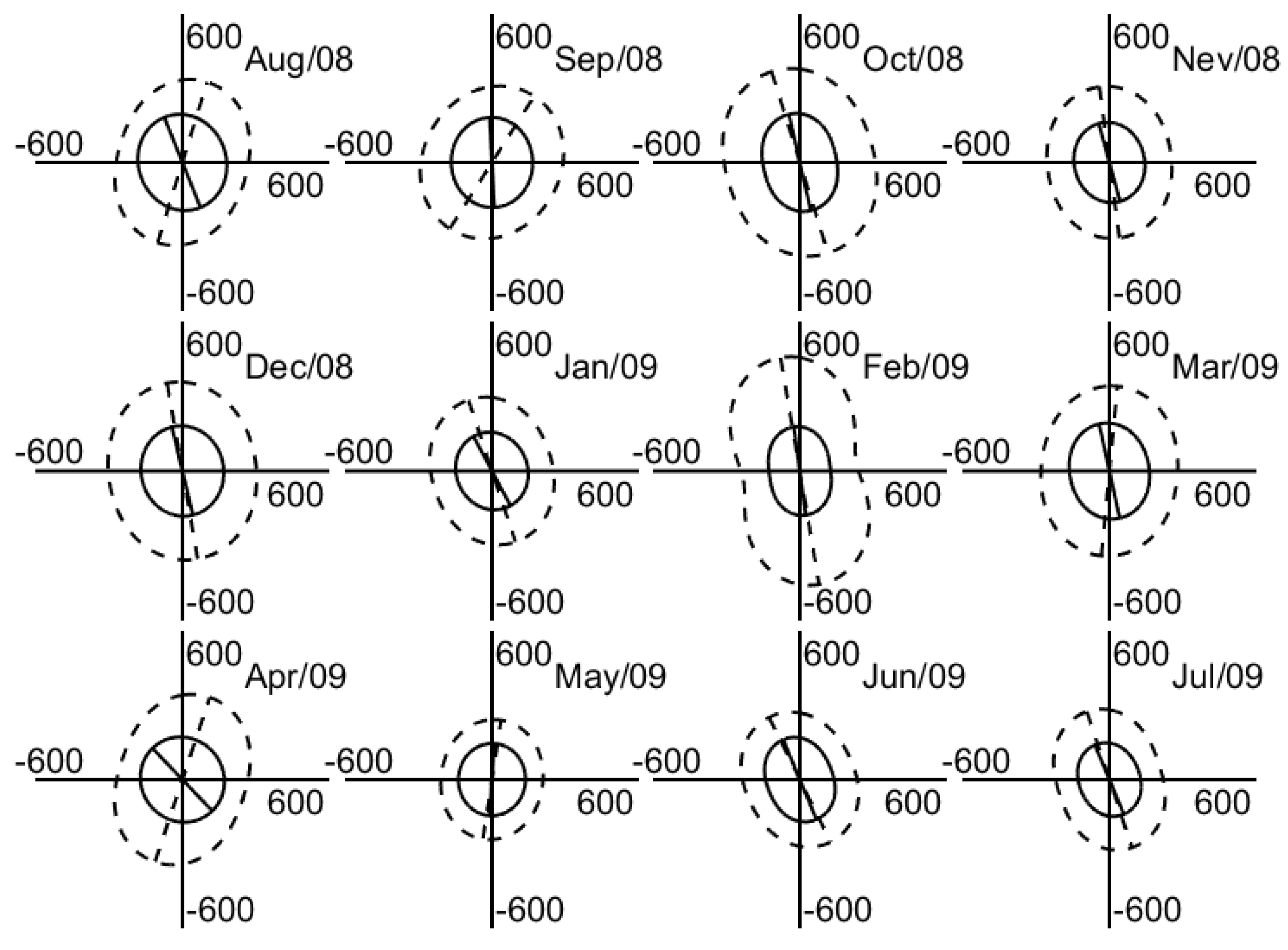
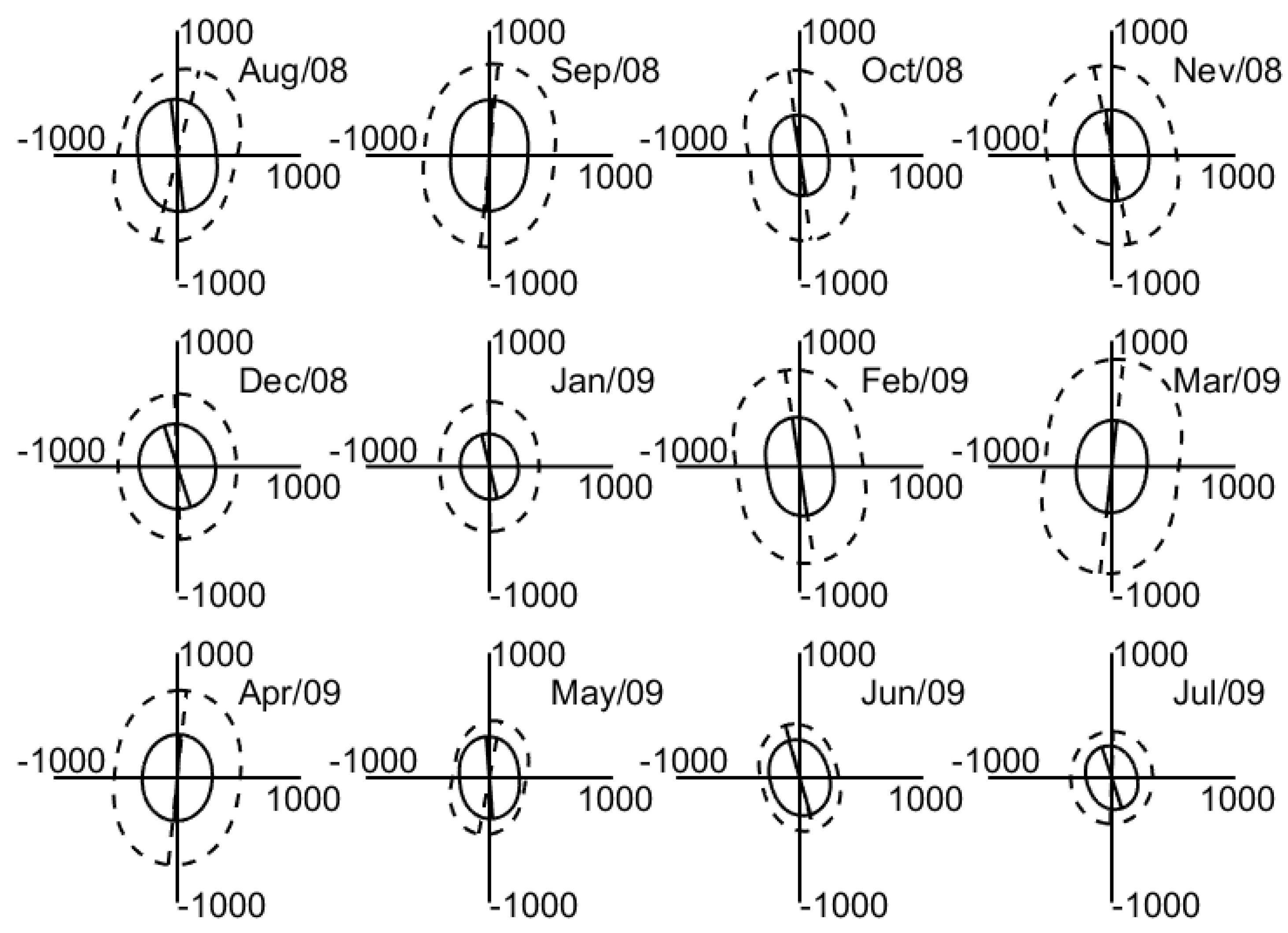
The propagating direction of GW in the mesosphere is free, and its direction varies in different months. To illustrate this point, the propagation directions of GW every month over Kunming observed using the MF radar between 82–90 km and 92–100 km are shown in Figure 8 and Figure 9. In them, the cycle means the GW packets and the large elliptical spindle implies the propagating direction of GW waves, while “600” in Figure 8 or “1000” in Figure 9 labeled at horizontal or vertical axis denote the wave velocity. As can be seen, at Kunming below 90 km, the GWs propagate mainly towards to northwest from June to July, October to February and northeast in other months. One point must be noted that the azimuthal propagating direction has no neglected differences, for instance, from October to February, although the propagating direction is northwest in these months. In detail, the azimuthal of propagating direction is largest in October and smallest in November. Moreover, the propagating direction in March is northeast, but the azimuthal is less than 5°. In a word, the propagating direction shows clear semiannual variation. Meantime, the wave intensity between the height of 82 and 90 km is largest in February with a maximum of 590 m2 s−2 and smallest in May with a maximum of 300 m2 s−2. The propagating direction shown in Figure 9 denotes that the major differences between lower and higher heights should be further understood. For example, the propagating direction is northeast at the height of 92–100 km as well as at the height of 82–90 km, while the azimuthal of the propagating direction is much smaller above 92 km.
It makes us glad that the propagating direction in December and January above 92 tends to be northern. The velocity of the GW wave is largest in March, with a maximum of about 900 m2 s−2, and smallest in July, with a minimum of about 400 m2 s−2. Likewise, semiannual variation in the GW wave above 92 km appears in the propagating direction and wave velocity, the same as that below 90 km shown in Figure 8.
A strong anisotropy with a majority of the waves propagating towards the north or the northeast can also be found in Figure 8 and Figure 9. Two main possible reasons have been taken into account to discuss this anisotropy: Taylor et al. (1993) proved that the upward flux of waves can be altered by the background wind depending upon their phase speeds and headings [42]. If the wind speed component being parallel to the direction of wave propagation becomes equal to the observed phase speed of this wave, the wave can be absorbed into the background medium and consequently prohibited from reaching higher altitudes. The so-called critical layer filtering mechanism may explain the strong anisotropy in the wave propagation seen from Stockholm.
Another possible reason for the anisotropy is the non-uniformity in the distribution of the source regions. Atmospheric GWs have different origins: orographic forcing by mountains, frontal zones, wave–wave interactions [4], or tropospheric convection. The Kunming area is located on the Yunnan–Guizhou Plateau; its latitude is 25.6° N, belonging to the subtropical region. Orographic forcing by mountains, frontal zones, and tropospheric convection may be the main sources. Short-period GWs originating from these types of sources can be accounted for this anisotropy in the propagation direction.
In combination with simulations using the GW resolving version of the mechanistic general circulation model KMCM [43], recent studies based on nearly identical radars at middle and high latitudes show the largest level of GW energy during winter and a secondary maximum during summer, which is more pronounced at middle latitudes [41]. Now, this behavior was found as typical for the activity of mesoscale GWs at middle and high latitudes, whereas short-period GWs are observed at some low latitudes [44,45] and showed equinoctial maxima.
It is noteworthy that GWs are normally observed as the superposition of waves with various frequencies and wavelengths. Each observation technique extracts only a part of the spectra because of limits to both time and height resolutions. Therefore, it is sometimes difficult to detect the difference in the GW energy obtained by using different observation techniques.
5. Summary
In this paper, numerical filters are used to derive GWs with the period of 0.1–1 h (so-called high frequency) and 1–5 h (so-called low frequency) to investigate the oscillations in GW wave activities around the mid-low latitude area. The interesting results are the following:
- (1)
- At Kunming area, the HF GWs act lively; the energy focuses on the waves with a period of <2 h. Meanwhile, the changes in power spectral density with the period of <2 h are almost linear as the decreasing frequency. Conversely, the decreasing gradient behaves gently as a decreasing frequency when its period is larger than 2 h.
- (2)
- The semiannual oscillation dominates the meridional GW variance below 90 km, and seasonal variation plays an important role in the meridional GW variance above 92 km and the zonal GW variance at all heights. For the GW variance with a period of <1 h, the variance is stronger in autumn and spring, with the maximum occurring in September, December, and March; moreover, the oscillations with a period of 30–90 days can also be found.
- (3)
- The behaviors of GW activity are consistent with that of turbulent velocity. The propagating direction of GW activity shows significant semiannual variation, and at the same time, the wave intensity is stronger above 92 km. Moreover, the propagating direction angle is rich.
Author Contributions
Conceptualization, N.L.; methodology, N.L. and J.C.; formal analysis, J.W.; resources, L.Z.; writing—original draft preparation, N.L. and J.C.; writing—review and editing, N.L., J.C. and G.H.; supervision, Z.D. All authors have read and agreed to the published version of the manuscript.
Funding
This research work was supported by the National Key Research and Development Plan of China (2022YFF0503700).
Institutional Review Board Statement
Not applicable.
Informed Consent Statement
Not applicable.
Data Availability Statement
The data used in this paper cannot be disclosed due to the utilizing restrictions of data according to the rules in China Research Institute of Radiowave Propagation. The data can be available upon the request.
Conflicts of Interest
The authors declare no conflict of interest.
References
- Zhang, J.; Xu, J.; Wang, W.; Wang, G.; Ruohoniemi, J.M.; Shinbori, A.; Nishitani, N.; Wang, C.; Deng, X.; Lan, A.; et al. Oscillations of the ionosphere caused by the 2022 Tonga volcanic eruption observed with SuperDARN radars. Geophys. Res. Lett. 2022, 49, e2022GL100555. [Google Scholar] [CrossRef]
- Chen, J.S.; Xu, L.L.; Ma, C.B.; Li, N.; Lin, L.K. A new method of determining momentum flux based on the all-sky meteor radar. Chin. J. Radio Sci. 2016, 31, 1124–1131. [Google Scholar]
- Andrews, D.G.; Holton, J.R.; Leovy, C.B. Middle Atmosphere Dynamics. In An Introduction to Dynamic Meteorology, 5th ed.; James, R.H., Gregory, J.H., Eds.; Academic Press: New York, NY, USA, 2013. [Google Scholar]
- Fritts, D.C.; Alexander, M.J. Gravity wave dynamics and effects in the middle atmosphere. Rev. Geophys. 2003, 41, 1003. [Google Scholar] [CrossRef]
- Kruse, C.G.; Alexander, M.J.; Bramberger, M.; Chattopadhyay, A.; Hassanzadeh, P.; Green, B.; Grimsdell, A.; Hoffmann, L. Recreating observed convection-generated GWs from weather radar observations via a neural network and a dynamical atmospheric model. Authorea Prepr. 2023, 97, 621–638. [Google Scholar]
- Franco-Diaz, E.; Gerding, M.; Holt, L.; Strelnikova, I.; Wing, R.; Baumgarten, G.; Lubken, F.J. Convective GW events during summer near 54N, present in both AIRS and RMR Lidar observations. Egusphere 2023. [Google Scholar] [CrossRef]
- Hoffmann, L.; Xue, X.; Alexander, M.J. A global view of stratospheric GW hotspots located with atmospheric infrared sounder 380 observations. J. Geophys. Res. Atmos. 2013, 118, 416–434. [Google Scholar] [CrossRef]
- Ern, M.; Hoffmann, L.; Rhode, S.; Preusse, P. The mesoscale GW response to the 2022 Tonga volcanic eruption: AIRS and MLS satellite observations and source backtracing. Geophys. Res. Lett. 2022, 49, e2022GL098626. [Google Scholar] [CrossRef]
- Zhang, K.; Wang, H.; Zhong, Y.; Xia, H.; Qian, C. The Temporal Evolution of F-Region Equatorial Ionization Anomaly Owing to the 2022 Tonga Volcanic Eruption. Remote Sens. 2022, 14, 5714. [Google Scholar] [CrossRef]
- Wang, H.; Xia, H.; Zhang, K. Variations in the Equatorial Ionospheric F Region Current during the 2022 Tonga Volcanic Eruption. Remote Sens. 2022, 14, 6241. [Google Scholar] [CrossRef]
- Zhang, S.-R.; Vierinen, J.; Aa, E.; Goncharenko, L.P.; Erickson, P.J.; Rideout, W.; Coster, A.J.; Spicher, A. 2022 Tonga Volcanic Eruption Induced Global Propagation of Ionospheric Disturbances via Lamb Waves. Front. Astron. Space Sci. 2022, 9, 871275. [Google Scholar] [CrossRef]
- Liu, J.Y.; Chen, C.H.; Sun, Y.Y.; Chen, C.H.; Tsai, H.F.; Yen, H.Y.; Chum, J.; Lastovicka, J.; Yang, Q.S.; Chen, W.S.; et al. The vertical propagation of disturbances triggered by seismic waves of the 11 March 2011 M9.0 Tohoku earthquake over Taiwan. Geophys. Res. Lett. 2016, 43, 1759–1765. [Google Scholar] [CrossRef]
- Plougonven, R.; de la Cámara, A.; Hertzog, A.; Lott, F. How does knowledge of atmospheric GWs guide their parameterizations? Q. J. R. Meteorol. Soc. 2020, 146, 1529–1543. [Google Scholar] [CrossRef]
- Cai, X.; Yuan, T.; Liu, H.-L. Large Scale Gravity Waves perturbations in mesosphere region above northern hemisphere mid-latitude during Autumn-equinox: A joint study by Na Lidar and Whole Atmosphere Community Climate Model. Ann. Geophys. 2017, 35, 181–188. [Google Scholar] [CrossRef]
- Li, J.; Lu, X. SABER observations of GW responses to the Madden-Julian Oscillation from the stratosphere to the lower thermosphere in tropics and extratropics. Geophys. Res. Lett. 2020, 47, e2020GL091014. [Google Scholar] [CrossRef]
- Fritts, D.C.; Vincent, R.A. Mesospheric momentum flux studies at Adelaide, Australia: Observations and a GW-tidal interaction model. J. Atmos. Sci. 1987, 44, 605–619. [Google Scholar] [CrossRef]
- Baumgarten, K.; Gerding, M.; Baumgarten, G.; Lübken, F.-J. Temporal variability of tidal and gravity waves during a record long 10-day continuous lidar sounding. Atmos. Chem. Phys. 2018, 18, 371–384. [Google Scholar] [CrossRef]
- Pramitha, M.; Kumar, K.K.; Ratnam, M.V.; Praveen, M.; Rao, S.V.B. GW source spectra appropriation for mesosphere lower thermosphere using meteor radar observations and GROGRAT model simulations. Geophys. Res. Lett. 2020, 47, e2020GL089390. [Google Scholar] [CrossRef]
- Matsumoto, N.; Shinbori, A.; Riggin, D.M.; Tsuda, T. Measurement of momentum flux using two meteor radars in Indonesia. Ann. Geophys. 2016, 34, 369–377. [Google Scholar] [CrossRef]
- Wu, Y.Y.; Tang, Q.; Chen, Z.; Liu, Y.; Zhou, C. Diurnal and Seasonal Variation of High-Frequency GWs at Mohe and Wuhan. Atmosphere 2022, 13, 1069. [Google Scholar] [CrossRef]
- Manson, A.H.; Meek, C.E.; Hall, G.E. Correlations of GWs and tides in the mesosphere over Saskatoon. J. Atmos. Sol.-Terr. Phys. 1998, 60, 1089–1107. [Google Scholar] [CrossRef]
- Gavrilov, N.M.; Riggin, D.M.; Fritts, D.C. Medium-frequency radar studies of gravity-wave seasonal variations over Hawaii (22N, 160W). J. Geophys. Res. Atmos. 2003, 108, 4655. [Google Scholar] [CrossRef]
- Appleton, E.V. Two anomalies in the ionosphere. Nature 1946, 157, 691. [Google Scholar] [CrossRef]
- Xiong, C.; Luhr, H.; Ma, S.Y. The magnitude and interhemispheric asymmetry of equatorial ionization anomaly-based on CHAMP and GRACE observations. J. Atmos. Sol.-Terr. Phys. 2013, 105–106, 160–169. [Google Scholar] [CrossRef]
- Immel, T.J.; Sagawa, E.; England, S.L. Control of equatorial ionospheric morphology by atmospheric tides. Geophys. Res. Lett. 2006, 33, L15108. [Google Scholar] [CrossRef]
- Hartman, W.A.; Heelis, R.A. Longitudinal variations in the equatorial vertical drift in the topside ionosphere. J. Geophys. Res. Space Phys. 2007, 112, A03305. [Google Scholar] [CrossRef]
- Luhr, H.; Hausler, K.; Stolle, C. Longitudinal variation of F region electron density and thermospheric zonal wind caused by atmospheric tides. Geophys. Res. Lett. 2007, 34, L16102. [Google Scholar] [CrossRef]
- Luhr, H.; Rother, M.; Hausler, K. The influence of nonmigrating tides on the longitudinal variation of the equatorial electrojet. J. Geophys. Res. Space Phys. 2008, 113, A08313. [Google Scholar] [CrossRef]
- Mo, X.H.; Zhang, D.H.; Goncharenko, L.P. Quasi-16-day periodic meridional movement of the equatorial ionization anomaly. Ann. Geophys. 2014, 32, 121–131. [Google Scholar] [CrossRef]
- Mo, X.H.; Zhang, D.H.; Goncharenko, L.P. Meridional movement of northern and southern equatorial ionization anomaly crests in the East-Asian sector during 2002–2003 SSW. Sci. China Earth Sci. 2017, 60, 776–785. [Google Scholar] [CrossRef]
- Mo, X.H.; Zhang, D.H. Lunar tidal modulation of periodic meridional movement of equatorial ionization anomaly crest during sudden stratospheric warming. J. Geophys. Res. Space Phys. 2018, 123, 1488–1499. [Google Scholar] [CrossRef]
- Zhao, L.; Chen, J.S.; Ding, Z.H.; Li, N.; Zhao, Z.W. First observations of tidal oscillations by an MF radar over Kunming (25.6N, 103.8E). J. Atmos. Sol.-Terr. Phys. 2012, 78–79, 44–52. [Google Scholar] [CrossRef]
- Li, N.; Chen, J.S.; Ding, Z.H.; Zhao, Z.W. Mean winds observed by the Kunming MF radar in 2008–2010. J. Atmos. Sol.-Terr. Phys. 2015, 122, 58–65. [Google Scholar] [CrossRef]
- Yi, W.; Chen, J.-S.; Ma, C.-B.; Li, N.; Zhao, Z.-W. Observation of Upper Atmospheric Temperature by Kunming All-Sky Meteor Radar. Chin. J. Geophys. 2014, 57, 750–760. [Google Scholar]
- Zeng, J.; Yi, W.; Xue, X.; Reid, I.; Hao, X.; Li, N.; Chen, J.; Chen, T.; Dou, X. Comparison between the Mesospheric Winds Observed by Two Collocated Meteor Radars at Low Latitudes. Remote Sens. 2022, 14, 2354. [Google Scholar] [CrossRef]
- Holdsworth, D.A.; Reid, I.M. Spaced antenna analysis of atmospheric radar backscatter model data. Radio Sci. 1995, 30, 1417–1433. [Google Scholar] [CrossRef]
- Royrvik, O. Spaced antenna drift at Jicamarca, mesospheric measurements. Radio Sci. 1983, 18, 461–476. [Google Scholar] [CrossRef]
- Manson, A.H.; Meek, C.E. GW Propagation Characteristics (60–120 km) as Determined by the Saskatoon MF Radar (Gravnet) System: 1983–85 at 52° N, 107° W. Atmos. Sci. 1988, 45, 932–946. [Google Scholar] [CrossRef]
- Reid, I.M.; Vincent, R.A. Measurement of the horizontal scales and phase velocities of short period mesospheric GWs at Adelaide, Australia. J. Atmos. Terr. Phys. 1987, 49, 1033–1048. [Google Scholar] [CrossRef]
- Hibbins, R.E.; Espy, P.J.; Jarvis, M.J.; Riggin, D.M.; Fritts, D.C. A climatology of tides and GW variance in the MLT above Rothera, Antarctica obtained by MF radar. J. Atmos. Sol.-Terr. Phys. 2007, 69, 578–588. [Google Scholar] [CrossRef]
- Hoffmann, P.; Becker, E.; Singer, W.; Placke, M. Seasonal variation of mesospheric waves at northern middle and high latitudes. J. Atmos. Sol.-Terr. Phys. 2010, 72, 1068–1079. [Google Scholar] [CrossRef]
- Taylor, M.J.; Ryan, E.H.; Tuan, T.F.; Edwards, R. Evidence of preferential directions for GW propagation due to wind filtering in the middle atmosphere. J. Geophys. Res. Space Phys. 1993, 98, 6047–6057. [Google Scholar] [CrossRef]
- Becker, E. Sensitivity of the upper mesosphere to the Lorenz energy cycle of the troposphere. J. Atmos. Sci. 2009, 66, 647–666. [Google Scholar] [CrossRef]
- Clemesha, B.R.; Batista, P.P.; da Costa, R.A.B.; Schuch, N. Seasonal variations in GW activity at three locations in Brazil. Ann. Geophys. 2009, 27, 1059–1065. [Google Scholar] [CrossRef]
- Antonita, T.M.; Ramkumar, G.; Kumar, K.K.; Deepa, V. Meteor wind radar observations of GW momentum fluxes and their forcing toward the Mesospheric Semiannual Oscillation. J. Geophys. Res. Atmos. 2008, 113, D10115. [Google Scholar] [CrossRef]
Figure 1.
The monthly averaged zonal wind observed via MF radar from August 2008 to July 2009 at Kunming.
Figure 1.
The monthly averaged zonal wind observed via MF radar from August 2008 to July 2009 at Kunming.

Figure 2.
Monthly frequency spectra for zonal winds (red dotted line) and meridional winds (blue solid line) from the Kunming MF radar. The dashed straight line has a slope of , and the vertical straight line indicates the period of 2 h.
Figure 2.
Monthly frequency spectra for zonal winds (red dotted line) and meridional winds (blue solid line) from the Kunming MF radar. The dashed straight line has a slope of , and the vertical straight line indicates the period of 2 h.

Figure 3.
The monthly HF meridional wind variances with timescales of 0.1–1 h over Kunming from August 2008 to July 2009. Contours are plotted at 200 m2 s−2 intervals.
Figure 3.
The monthly HF meridional wind variances with timescales of 0.1–1 h over Kunming from August 2008 to July 2009. Contours are plotted at 200 m2 s−2 intervals.

Figure 4.
The same as Figure 3, but for zonal variance.
Figure 4.
The same as Figure 3, but for zonal variance.

Figure 5.
The monthly LF meridional wind variances with timescales 1–5 h over Kunming from August 2008 to July 2009. Contours are plotted at 50 m2 s−2 intervals.
Figure 5.
The monthly LF meridional wind variances with timescales 1–5 h over Kunming from August 2008 to July 2009. Contours are plotted at 50 m2 s−2 intervals.

Figure 6.
The same as Figure 5, but for zonal variance.
Figure 6.
The same as Figure 5, but for zonal variance.

Figure 7.
The variation of turbulent velocity observed by the Kunming MF radar between August 2008 and July 2009.
Figure 7.
The variation of turbulent velocity observed by the Kunming MF radar between August 2008 and July 2009.

Figure 8.
The propagation direction of GW over Kunming observed by the MF radar between 82–90 km.

Figure 9.
The same as Figure 8, but for 92–100 km.
Figure 9.
The same as Figure 8, but for 92–100 km.


Table 1.
Main specifications of the Kunming MF radar.
| Location | 25.6° N, 103.8° E |
| Operation frequency | 2.138 MHz |
| Peak envelope power | 64 kW |
| Half-power pulse width | 21.33 μs |
| Antenna spacing | 170 m |
| Range resolution | 3.2 km |
| Sampling interval | 2 km |
| Time resolution | 3 min |
| Antenna | 4 cross dipoles (for Tx and Rx) |
Table 2.
The details about FCA method of Kunming MF radar.
| Parameter | Day Value | Night Value |
|---|---|---|
| Height resolution | 2 km | 2 km |
| Start range | 50 km | 50 km |
| Polarization | O-mode | E-mode |
| PRF | 80 Hz | 40 Hz |
| Coherent integrations | 32 | 16 |
| Number of samples | 285 | 285 |
| Record length | 114 s | 114 s |
Disclaimer/Publisher’s Note: The statements, opinions and data contained in all publications are solely those of the individual author(s) and contributor(s) and not of MDPI and/or the editor(s). MDPI and/or the editor(s) disclaim responsibility for any injury to people or property resulting from any ideas, methods, instructions or products referred to in the content. |
© 2023 by the authors. Licensee MDPI, Basel, Switzerland. This article is an open access article distributed under the terms and conditions of the Creative Commons Attribution (CC BY) license (https://creativecommons.org/licenses/by/4.0/).
Share and Cite
MDPI and ACS Style
Li, N.; Chen, J.; Wang, J.; Zhao, L.; Ding, Z.; He, G. Oscillations of GW Activities in the MLT Region over Mid-Low-Latitude Area, Kunming Station (25.6° N, 103.8° E). Atmosphere 2023, 14, 1810. https://doi.org/10.3390/atmos14121810
AMA Style
Li N, Chen J, Wang J, Zhao L, Ding Z, He G. Oscillations of GW Activities in the MLT Region over Mid-Low-Latitude Area, Kunming Station (25.6° N, 103.8° E). Atmosphere. 2023; 14(12):1810. https://doi.org/10.3390/atmos14121810
Chicago/Turabian StyleLi, Na, Jinsong Chen, Jianyuan Wang, Lei Zhao, Zonghua Ding, and Guojin He. 2023. "Oscillations of GW Activities in the MLT Region over Mid-Low-Latitude Area, Kunming Station (25.6° N, 103.8° E)" Atmosphere 14, no. 12: 1810. https://doi.org/10.3390/atmos14121810
Note that from the first issue of 2016, this journal uses article numbers instead of page numbers. See further details here.