Analysis of Changes in Rainfall Concentration over East Africa

Abstract

Understanding the spatial and temporal distribution of precipitation is important in agriculture, water management resources, and flood disaster management. The present study analyzed the changes in rainfall concentration over East Africa (EA). Three matrices—the precipitation concentration index (PCI), the precipitation concentration degree (PCD), and the precipitation concentration period (PCP)—were used to examine the changes in rainfall during 1981–2021. The changes in spatial variance annually and during two seasons, namely, “long rains” (March to May [MAM]) and “short rain” (October to December [OND]), were estimated using an empirical orthogonal function (EOF). The study employed the robust statistical metrics of the Theil–Sen estimator to detect the magnitude of change and modified Mann–Kendall (MMK) to examine possible changes in rainfall concentration. The localized variation of the power series within the series for PCI, PCD, and PCP variability was performed using the continuous wavelet transform. The findings showed that the concentration of rainfall patterns of EA occurred in four months of the total months in a year over most parts, with the western sides experiencing uniform rainfall events throughout the year. The EOF analysis revealed a homogeneous negative pattern during the MAM season over the whole region for PCD, PCI, and PCP for the first mode, which signified reduced rainfall events. Moreover, the MMK analysis showed evidence of declining trends in the PCD annually and during the MAM season, while the opposite tendency was noted for the OND season where an upward trend in the PCD was observed. Interestingly, areas adjacent to Lake Victoria in Uganda and Lake Tanganyika in Tanzania showed increasing trends in the PCD for annual and seasonal time scales. The analysis to characterize the rainfall cycle and possible return period, considering the indices of PCD, PCI, and PCP, showed higher variability during the year 2000, while much variability was presented in the PCP for the annual period. During the MAM and OND seasons, a 1-year band as a dominant period of variability was observed in all the indices. Overall, the findings of the present study are crucial in detecting the observed changes in rainfall concentration for avoiding the loss of life and property, as well as for coping with potential changes in water resources.

1. Introduction

The uneven spatial and temporal distribution of precipitation exacerbated by climate change has attracted much attention [1]. Understanding this distribution of precipitation is important in climate-sensitive sectors such as agriculture, water, and health. Some researchers have argued that the changes in precipitation concentration represent seasonal characteristics of precipitation [2,3]. The variation of precipitation concentration is critical to water resource utilization, and it affects human life, the environment, and the ecosystem. For instance, the change in precipitation concentration is important to adjust the optimal allocation scheme of soil and water resources in time and to ensure higher crop yields [3]. Intense rainstorms and floods as a result of a higher proportion of precipitation on rainy days to the total annual precipitation trigger landslides, mudslides, and urban logging [3,4]. Therefore, it is important to investigate the changes in precipitation concentration before devising the right structural and design measures to minimize loss of life and property.

Three types of statistical indices have been widely used to quantify the precipitation concentration in a year, based on monthly precipitation. Oliver [5] proposed a precipitation concentration index (PCI) that was later modified by de Luis [6]. The PCI is generally used for quantifying the distribution of the precipitation pattern and calculating seasonal precipitation changes. In addition, Zhang and Qian [7] proposed the precipitation concentration period (PCP) and the precipitation concentration degree (PCD) to investigate the concentration characteristics of precipitation. The PCP explains the period (month) in which the total precipitation within a year concentrates. The PCD represents the degree to which the total annual precipitation is concentrated over 12 months. Previous studies have examined the characteristics of precipitation concentration over various subregions in Africa [8,9,10,11,12]. For instance, Njouenwet et al. [10] analyzed spatial and temporal variations of PCI, PCP, and PCD in the Sudano–Sahelian region of Cameroon. The study found lower annual PCI values in the south and higher values in the far north. The PCP results indicated a slightly later occurrence of precipitation, with values increasing from the far north to the south.

In East Africa (EA), previous studies have employed various statistical approaches to define homogeneous regions and annual precipitation distributions. For instance, some studies [13,14] defined the seasonality of rainfall patterns based on the percentage ratio of each monthly rainfall to the total annual rainfall. On this basis, the long rainy (March to May [MAM]), short rainy (October to December [OND]), summer (June to August [JJA]), and winter (January to February [JF]) precipitation seasons can also be represented as a ratio of the precipitation amount in relation to the annual total (e.g., [14]). The statistical methods used to map the annual distribution of regional precipitation have a common limitation, that is, they are not able to indicate the annual PCD and the period of maximal precipitation.

The East Africa region continues to suffer sustained drought and flood episodes over the past decades that have led to massive changes in water levels for sustained livelihoods. Moreover, the evidence of increased temperatures due to global warming has led to increased evapotranspiration that threatens agriculture and ecological life due to reduced soil moisture. In fact, since 1992, the abrupt decline in the long rainy seasons has resulted in increased drought occurrences and subsequent changes in the degree of rainfall concentration [15,16,17]. However, existing studies have mainly focused on estimating the observed and projected changes in the weather and climate extreme events that result in floods or droughts over the study region [18,19,20,21,22,23,24]. These studies have provided useful information regarding the observed/projected changes in extreme climatic events. However, few studies have mainly focused on quantifying the changes in precipitation concentration, represented not only by higher percentages of the annual total precipitation in a few very rainy days but also the time and degree of concentration of the yearly/seasonal total rainfall within a year, which has a potential to cause the floods or droughts.

Knowledge about precipitation concentration changes, which is the main source of surface water over EA, is extremely important to determine the contribution of the days of the greatest rainfall to the total amount. Moreover, the livelihood of the regional population is sustained by rainfed agriculture, which consumes more than 90% of the water in the region [25]. If the PCP does not match the timing of agriculture irrigation, uneven precipitation concentrations may lead to difficulties in terms of water resource management. In addition, it is also imperative to understand the PCP and the PCD for the management of water resources. The evidence of climate change depicting a shift from warm–wet to warm–dry over the last two decades over EA as the globe is becoming warmer also poses more threats. Thus, there is a need to quantify the rainfall concentration and identify regions that have enough water levels for adequate planning and use. To the best of our knowledge, however, there has been no comprehensive study of precipitation concentration changes, either spatially or temporally, in EA. Therefore, the objective of this study was to analyze changes in the PCI, PCD, and PCP in EA using a monthly precipitation dataset. The results of this study may provide important and valuable information on water management and environmental problems for EA. The rest of the paper is organized as follows: Section 2 presents detailed information about the study domain, the data acquisition procedure and processing, and the methods used. Section 3 highlights results and discussion, while the last section contains key conclusions and recommendations for future studies.

2. Materials and Methods

2.1. Study Area and Datasets

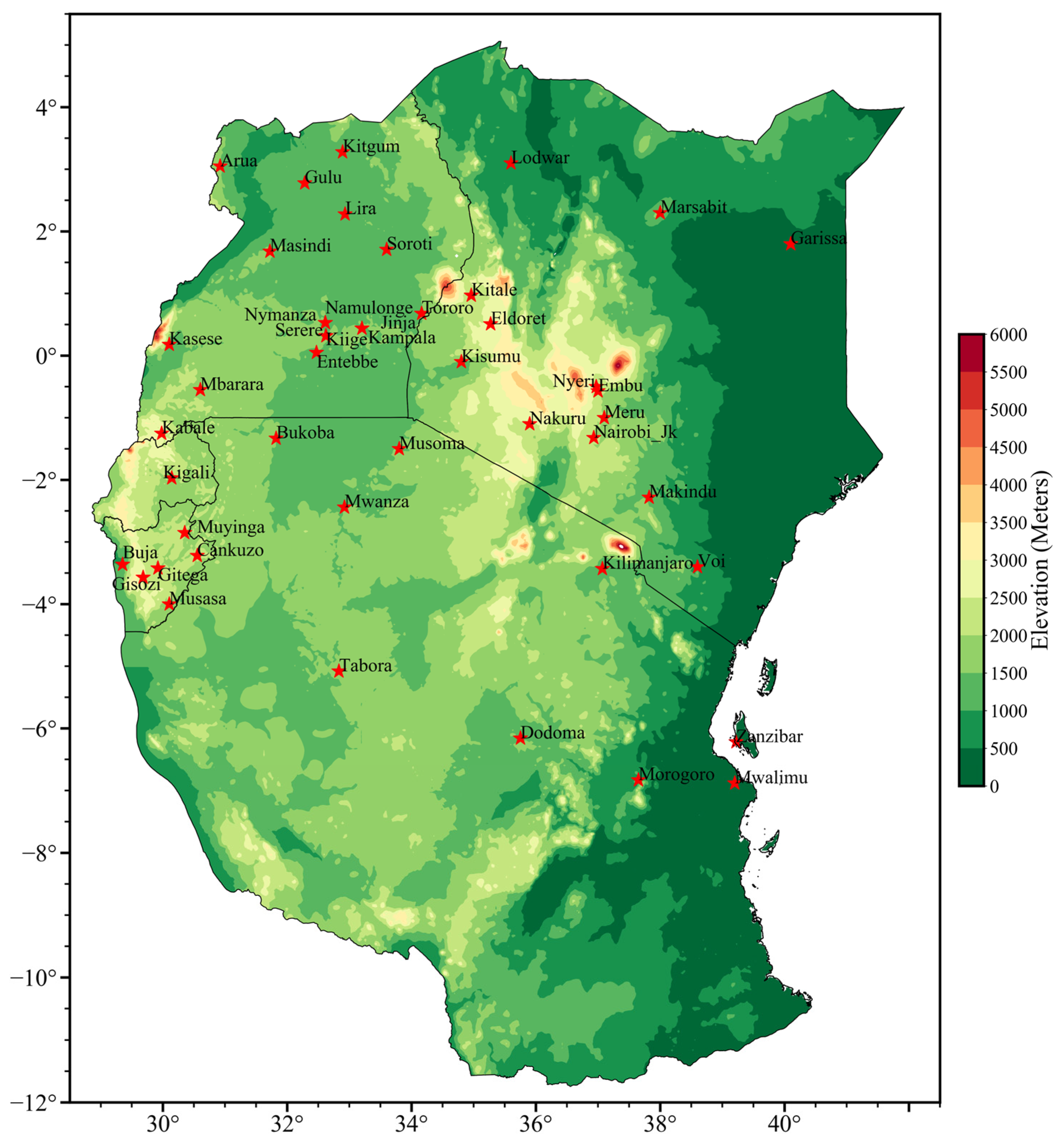
This study focused on the region of East Africa (EA), defined along the longitude 28°–40° E and latitude 12° S–5° N. The region encloses five countries: Kenya, Uganda, Tanzania, Burundi, and Rwanda. Somalia to the east, Ethiopia and Sudan on the Northern Horn of Africa, and South Sudan along the north of Uganda are part of the Greater Horn of Africa.

EA is characterized by large water bodies and complex topography such as Mount Kilimanjaro, Mount Kenya, and Mount Ruwenzori that controls the regional climate and socioeconomic activities. Other features include the long stretch of the 6000 km Rift Valley System, the vast dry anomaly landscape of Arid and Semi-Arids (ASALs) desert in the otherwise wet equatorial belt zone, and the large coastlines of the Indian Ocean and inland water bodies of lakes and rivers [26]. It should be noted that the vast valleys within the EA region, such as the Turkana Basin in Kenya, are mainly responsible for the dry anomaly and ASAL climate due to their role in channeling the water vapor toward the Congo Basin rainforest [27]. The regions receive two main rainfall seasons during MAM and OND [28]. The two seasons are regulated by the oscillation of the tropical rain belt along 15° S to 15° N, which brings with it enhanced moisture convergence from easterly and westerly flows [29]. Other factors that regulate the variability of climate include global teleconnections such as the El Nino Southern Oscillation [30], the Indian Ocean Dipole [31,32], the Madden–Julian Oscillation [33], and sub-tropical high-pressure systems [31,34]. Despite the complex features, the region is marred by the occurrence of extreme climate events, such as recurrent drought episodes that threaten agricultural activities and hydrological groundwater levels [17,35]. In recent years, the region has experienced multiple rainfall anomalies and high temperatures, leading to devastating droughts [29,36]. This calls for the need to re-examine the concentration of rainfall over the region for better planning purposes.

Monthly rainfall datasets spanning from 1981 to 2021 were sourced for 46 synoptic stations distributed across the EA. Initially, datasets from 57 stations were collected mostly from the Kenya Meteorological Department, Uganda National Meteorological Authority, Rwanda Meteorological Agency, Geographical Institute of Burundi, and Tanzania Meteorological Agency. However, the number of stations was reduced to the current number after data quality control. A summary of the station used, the geographical coordinates, the elevation (m), and the mean rainfall with the statistical values of the homogeneity test is presented in Figure 1 and

Table 1. Geographical coordinates for the selected 46 meteorological stations across East Africa; the mean seasonal rainfall (mm) values for each station are also listed in the table in addition to the statistical values of the Standard Normal Homogeneous Test (SNHT).

No.	Station	Lon (°E)	Lat (°N)	Elevation (m)	Precipitation (mm)			SNHT
					Annual	MAM	OND
1	Arua	30.92	3.05	1211	236.6	526.5	134.1	0.0113
2	Buja	29.35	3.36	774	96.46	135.97	126.18	0.513
3	Bukoba	31.82	−1.33	1144.2	87.86	102.31	143.75	0.001
4	Cankuzo	30.55	−3.22	1652	98.04	147.49	129.06	0.25
5	Dodoma	35.75	−6.16	1103.1	34.18	36.52	39.04	0.01
6	Eldoret	35.27	0.51	2184	51.99	30.46	65.43	0.01
7	Embu	37	−0.57	1905	89.39	131.26	158.28	0.065
8	Entebbe	32.47	0.05	1117.0	94.33	143.08	236.17	0.02
9	Garissa	40.10	1.80	246	31.46	57	44.08	0.174
10	Gisozi	29.68	−3.57	2097	121.60	166.92	165.23	0.3948
11	Gitega	29.92	−3.42	1524.3	96.07	135.97	126.18	0.51
12	Gulu	32.28	2.78	1025	124.16	117.46	137.9	0.58
13	Jinja	33.20	0.44	1175.2	108.31	129.28	155.04	0.8074
14	Kabale	29.98	−1.25	1743	85.27	108.79	115.23	0.9178
15	Kampala	32.62	0.32	1162.0	114.99	145.51	150.87	0.003
16	Kasese	30.10	0.18	931.2	72.05	95.3	99.69	0.2324
17	Kigali	30.14	−1.97	1491	57.03	73.52	83.5	0.01
18	Kiige	32.62	0.32	1089.1	111.21	118.05	169.93	0.001
19	Kilimanjaro	37.07	−3.43	896	34.07	36.76	65.16	0.0268
20	Kisumu	34.8	−0.10	1154.3	98.29	104	145.77	0.01
21	Kitale	34.96	0.97	1875	101.79	89.46	137.98	0.0433
22	Kitgum	40.79	8.44	950	117.69	130.29	129.95	0.4294
23	Lira	32.93	2.28	1120.4	120.70	113.59	143.83	0.1188
24	Lodwar	35.60	3.10	515.0	19.46	17.69	33.91	0.0009
25	Makindu	37.82	−2.28	1000	30.95	64.86	33.71	0.01
26	Marsabit	38	2.30	1283	43.01	63.65	83.25	0.01
27	Masindi	31.72	1.68	1136.0	110.71	121.21	139.19	0.91
28	Mbarara	30.60	−0.55	1408.1	78.46	108.46	96.58	0.796
29	Meru	37.10	−1.0	1531	101.12	208.94	136.26	0.0175
30	Morogoro	37.65	−6.83	526	41.56	37.12	84.33	0.02
31	Musasa	30.10	−4	1950	92.23	125.28	132.69	0.9156
32	Musoma	33.80	−1.50	1147	44.19	53.73	79.82	0.01
33	Muyinga	30.35	−2.85	1745	91.15	127.04	134.06	0.8324
34	Mwalimu	39.20	−6.88	55	89.53	100.83	173.23	0.2509
35	Mwanza	32.92	−2.44	1139	58.91	86.44	83.33	0.01
36	Nairobi_JKIA	36.93	−1.32	1624	61.51	82.07	101.49	0.4577
37	Nakuru	35.90	−1.10	1890	74.46	73.37	98.23	0.1017
38	Namulonge	32.61	0.53	1128.3	93.44	107.53	126.46	0.4194
39	Nyeri	36.97	−0.50	2372	70.32	95.4	118.96	0.01
40	Nymanza	32.61	0.53	3810	97.50	147.44	134.89	0.6138
41	Serere	32.62	0.32	1098.2	110.12	86.42	158.14	0.9294
42	Soroti	33.60	1.71	1115.1	113.20	94.85	147.58	0.5939
43	Tabora	32.83	−5.08	1215.0	52.34	82.81	59.83	0.001
44	Tororo	34.16	0.68	1176.0	125.33	128.4	189.12	0.01
45	Voi	38.60	−3.4	579.0	46.09	90.47	58.44	0.0641
46	Zanzibar	39.22	−6.22	15	72.69	98.3	137.17	0.01

.

2.2. Methods

2.2.1. Computation of PCI, PCD, and PCP

The PCI introduced by Oliver [5] is a metric that is used to analyze intra-annual precipitation variability and can measure relationship between distribution and variability of monthly precipitation. The PCI was computed at each grid point using Oliver’s [5] approach (Equation (1)):

$$\mathrm{PCI}=\frac{{{\displaystyle \sum }}_{i=1}^N{p}_i^2}{{\left({{\displaystyle \sum }}_{i=1}^N{p}_i\right)}^2}\times 100$$

(1)

$$\mathrm{PCI}=\frac{{{\displaystyle \sum }}_{i=1}^N{p}_i^2}{{\left({{\displaystyle \sum }}_{i=1}^N{p}_i\right)}^2}\times \frac{100\times mon}{12}$$

(2)

where $p_i$ refers to the precipitation total (mm) in the $i^{th}$ month. The computation of PCI can be performed in three ways; mon represents the number of months in each season.

The mean of the precipitation total for each month over the data period was separately computed to obtain a total of twelve (12) $p_i$ values. Next, Equation (1) was applied with the term $N$ set to 12 (or the number of months in a year). We refer to this as the seasonal PCI (PCI_seasonal). The application of this method to data at every grid point was to show the spatial precipitation distribution across the study area in each month.

Equation (1) was applied to the monthly precipitation of each year separately. Here the number of PCI values was equal to the data record length in years. This approach was termed the temporal monthly PCI and was used to determine the variation of the seasonal PCI with time. While Equation (2) was applied on a seasonal scale based on the wet seasons of MAM and OND, respectively, the monthly precipitation was averaged over each year, Equations (1) and (2) were applied to the annual and seasonal precipitation series with $N$ taken as the length of the precipitation record in years, and we obtained the annual PCI. The application of this approach was to highlight the spatial variation in the annual PCI across the study area. At a particular location, the annual PCI provides an indication of the temporal precipitation concentration. The interpretation of the PCI values depends on the time scale, as shown in

Table 2. Classification of PCI values [5,37].

SNo	PCI Value	PCI Season	PCI Annual
1	≤10	Uniform	Uniform
2	11–15	Moderate seasonal	Moderately concentrated
3	16–20	Seasonal	Concentrated
4	>20	Strong seasonal	Strong concentrated

.

Considering that monthly precipitation comprises both the magnitude and the direction and can be termed to be a vectoral quantity [38,39], two other indices, including the PCD and the PCP, were proposed by Zhang and Qian [7]. As a vectoral quantity, the precipitation total was taken as the magnitude of the vector. The direction was given in terms of an angle (θ) assigned to each month with 30° increments (

Table 3. Angle of each month for computing PCP and PCD [7].

Month	January	February	March	April	May	June	July	August	September	October	November	December
θ	0°	30°	60°	90°	120°	150°	180°	210°	240°	270°	300°	330°

).

Consider that $h_{ij}$ stands for the monthly precipitation total in the $j^{th}$ month and $i^{th}$ year. $PC{D}_{ij}$ refers to the degree to which the total precipitation of the $i^{th}$ year concentrates in 12 months. On the other hand, $PC{P}_{ij}$ denotes the period (month) over which the total precipitation of the $i^{th}$ year concentrates. $PC{D}_{ij}$ and $PC{P}_{ij}$ were computed using [7].

$$R_i=\sum h_{ij}$$

(3)

$$R_{xi}=\sum h_{ij}·cos{\theta }_j$$

(4)

$$R_{yi}=\sum h_{ij}·sin{\theta }_j$$

(5)

$${\mathit{PCP}}_{ij}=arctan\left(R_{xi}/R_{yi}\right)$$

(6)

$${\mathit{PCD}}_{ij}=\sqrt{R_{xi}^2+(R_{yi}/R_i)}$$

(7)

The computed long-term mean of the $PC{D}_{ij}$ and $PC{P}_{ij}$, values obtained using Equations (6) and (7) can be averaged over the data record period. Equations (6) and (7) were applied at annual and seasonal scales (MAM and OND).

For the spatial representation of the PCD, PCI, and PCP, the indices were spatially interpolated using the Kriging interpolation method. The built-in package in Python software was used for this purpose. The Kriging method measures how similar close stations are in value and how this similarity changes as the distance between stations increases (spatial autocorrelation); the same method was used by [10].

2.2.2. Spatial Variation in PCI, PCD, and PCP

An investigation of variability using an empirical orthogonal function (EOF) [40,41] was conducted using covariance matrix of PCI, PCD, and PCP anomalies. The EOF allows the extraction of time-dependent spatial modes of variability by generating the decomposition from a dataset using orthogonal basis functions. It yields spatial structures (EOFs) and corresponding principal component $\left(C_n\right)$ time series. Thus, space–time data $X\left(g,t\right)$ can be characterized in terms of the loading vectors $\left(Q_n\right)$ and their $C_n$ time series:

$$X\left(g,t\right)={\displaystyle \sum }_n{C}_n\left(t\right)Q_n\left(g\right)$$

(8)

The EOFs (or spatial patterns) and temporal patterns (or ${C_n}^{\prime }s$) are orthogonal in their own dimension [42]. Furthermore, the EOFs occur in an ordered magnitude. The temporal patterns in terms of the $C_n$ time series are expected to oscillate over time. Loading vectors indicate independent variability patterns from the given series, and their interpretations can be linked to the physical model of the system from which the series were derived [43]. Given the sampling errors based on each eigenvector [41] and coupled with the suggestion that EOF beyond the second mode represents noise [42,44], this study considered the spatial and temporal patterns of the first two leading EOF modes (EOF1 and EOF2).

2.2.3. Trends in PCI, PCD, and PCP

The magnitude ($m$) of the trend in any of the series for PCI, PCD, and PCP was determined based on the method of Theil [45] and Sen [46] such that

$$m=median\left(\frac{x_j-x_i}{j-i}\right), \forall i<j$$

(9)

where $x_j$ and $x_i$ denote the $j^{th}$ and $i^{th}$ observations, respectively.

For determining the significance of trends, several non-parametric or rank-based approaches exist such as the Mann–Kendall test (MKT) [47,48], Spearman’s rho test (SRT) [49,50], and the Onyutha trend test (OTT) [51]. The comparability of MKT and SRT [52], as well as MKT and OTT [43], was demonstrated under various circumstances of variability, sample sizes, and trend slopes. For brevity, this study applied the MKT to test the null hypothesis H0 (no trend) using the statistic $S$ [47,48];

$$S={{\displaystyle \sum }}_{i=1}^{n-1}{{\displaystyle \sum }}_{j=1+1}^{n}sgn\left(x_j-x_i\right)$$

(10)

where $x_j$ and $x_i$ denote sequential values in a series of a sample of size $n$ and the values of $sgn\left(x_j-x_i\right)$ are taken to be $1, 0,$ and $-1$ in the cases when we obtain $\left(x_j-x_i\right)$ as $>0, 0,$ and $<0,$ respectively. The distribution of $S$ in the absence of data ties is approximately normal with the mean equal to zero and variance $V\left(S\right)$ given by

$$V\left(S\right)=\frac{1}{18} n\left(n-1\right)\left(2n+5\right)$$

(11)

The variance of $S$ corrected from the effect of autocorrelation (denoted by $V^{\prime }\left(S\right)$) was given by [53] $V^{\prime }\left(S\right)=V\left(S\right)\times (n/n^{\ast })$ such that

$$\frac{n}{n^{\ast }}=1+\frac{2}{n\left(n-1\right)\left(n-2\right)}\times {{\displaystyle \sum }}_{i=1}^{n-1}\left(n-i\right)\left(n-i-1\right)\left(n-i-2\right)\rho \left(i\right)$$

(12)

where $\rho \left(i\right)$ is the autocorrelation function of data ranks.

The standardized $S$ (denoted by $Z)$, which follows a standard normal distribution, was given by Equation (13):

$$Z=\left\{\begin{array}{c}\frac{S - 1}{\sqrt{V^{\prime }\left(S\right)}} \mathrm{for} S>0 \\ 0 \mathrm{for} S=0\\ \frac{S + 1}{\sqrt{V^{\prime }\left(S\right)}} \mathrm{for} S<0 \end{array}\right.$$

(13)

Positive and negative values of $S$ indicate increasing and decreasing trends, respectively. The H0 (no trend) was not rejected when $Z$ was less than the standard normal variate $Z_{\alpha }$, where $\alpha$ is the significance level, and it was taken to be 0.05.

2.2.4. Periodic Characteristics in PCI, PCD, and PCP

The PCI, PCD, and PCP were decomposed into time–frequency modes of variability using the continuous wavelet transform (CWT, Morlet wavelet), to analyze localized variation of the power series within the series [54]. Consider $x_n$ as a series with an equal time spacing ($\delta t$). Furthermore, take ${\phi }_0\left(\beta \right)$ as a wavelet function that depends on a dimensionless “time” $\beta$ with zero mean and is localized in both time and frequency [54,55]. The Mortet wavelet can be given by Equation (14):

$${\phi }_0\left(\beta \right)={\pi }^{-1/4}{e}^{i\omega \beta }{e}^{-{\beta }^2/2}$$

(14)

where $\omega$ denotes the non-dimensional frequency, and it is normally taken to be 6 to fulfill the admissibility condition [54,55]. The continuous wavelet transform $W_n\left(s\right)$ of $x_n$ with a scaled ${\phi }_0\left(\beta \right)$ is given by Equation (15):

$$W_n\left(s\right)={{\displaystyle \sum }}_k^{n-1}{x}_k\phi \times \left(\frac{\left(k-n\right)\delta t}{s}\right)$$

(15)

where (∗) represents the complex conjugate. Further details of this method can be found in [54].

3. Results and Discussions

3.1. EOF Analyses of PCD, PCI, and PCP

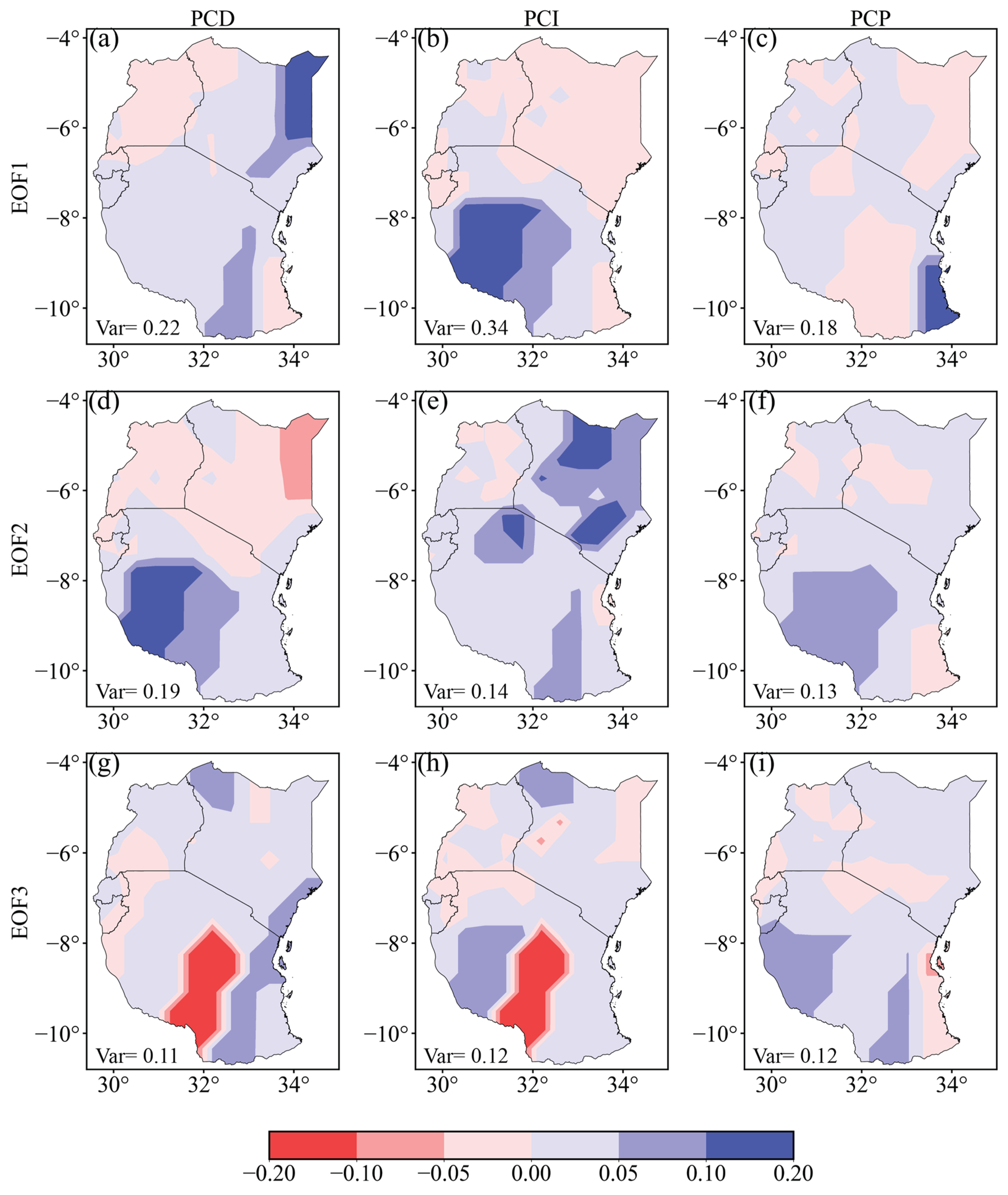
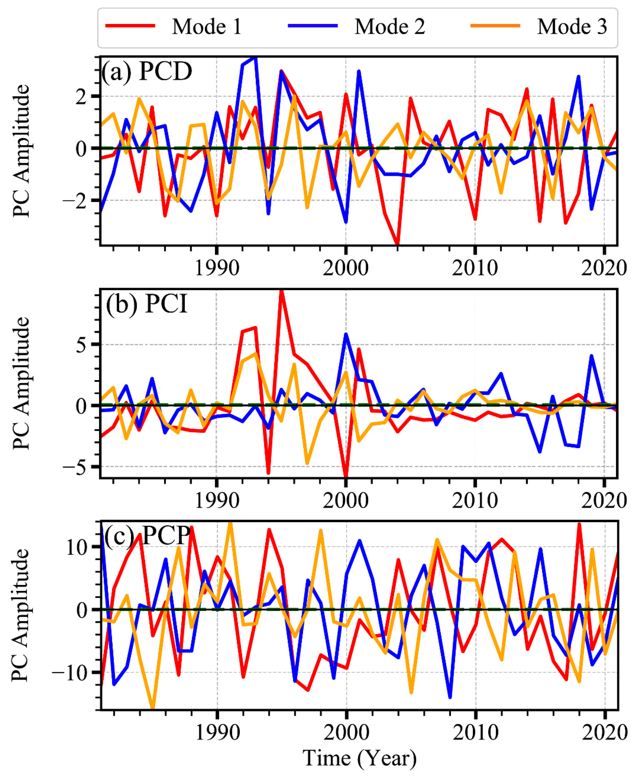
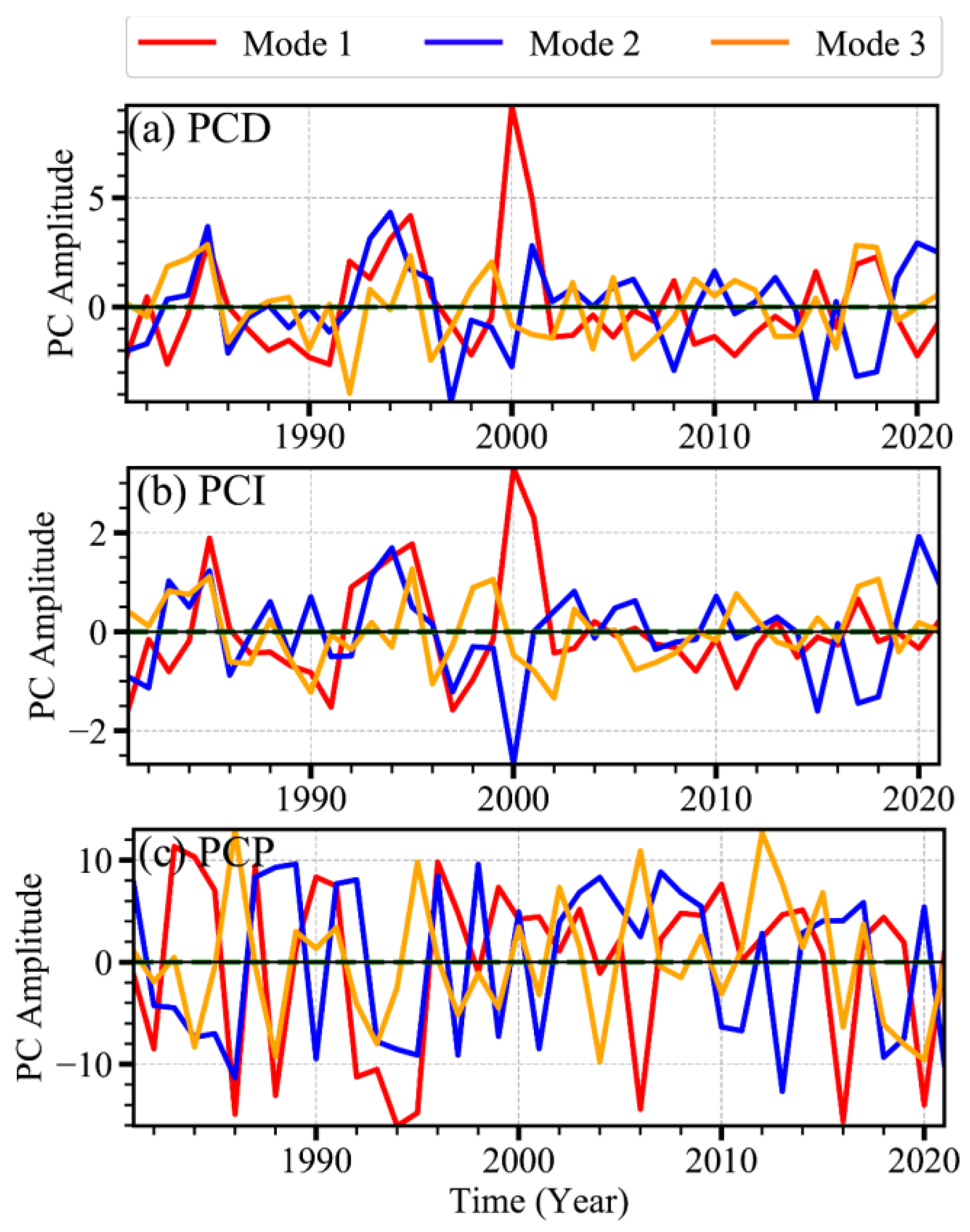
First, the study assessed the variation of the rainfall indices of PCI, PCD, and PCP over East Africa using an EOF. Figure 2 and Figure 3 show the spatial variance of the EOF analysis and the corresponding principal component (PC) denoting the years of anomalous events over the study region. The first three EOF modes of PCD accounted for 22%, 19%, and 11%. Mode 1 was predominantly depicting positive loadings over most parts of the region for PCD, with only the western region of Uganda showing negative loadings. Still on EOF mode 1, the study noted strong positive loadings over northeastern Kenya and southern parts of Tanzania, signifying the likelihood of a strong concentration of annual total rainfall during the last 12 months (Figure 2a). On the other hand, annual PCD modes 2 and 3 showed distinct variation in the spatial patterns over EA. For instance, mode 2 depicted considerably negative loadings over the entire Kenyan region and Uganda, while the southern parts of Tanzania were characterized by noteworthy positive loadings (Figure 2d). For EOF3, the results displayed almost similar variance to that of EOF1, except for the Tanzania region that demonstrated opposite loadings (Figure 2g). Meanwhile, the PCs for the first three modes showed interannual variability of the PCD, with years where the PCD was depicting positive/negative anomalies (Figure 3a). For instance, mode 1 showed several peaks during 1984, 1992, 1996, 1999, 2004, 2005, 2008, 2000, and 2014. These years denoted anomalous wet/dry conditions when the degree of the rainfall concentration during the whole year was below or above the normal thresholds.

The PCI results (Figure 2b,e,h), showed that the first three modes accounted for a total of 60% of the variance with leading mode 1 showing 34% area variance. The positive changes in PCI were predominant over the Tanzania region during mode 1, while mode 2 illustrated overall positive loadings over the entire region. Meanwhile, mode 3 showed general negative loadings over the entire domain, almost similar to those of mode 1, except for the Tanzania region. These results signified that various drivers influencing the spatiotemporal patterns for the PCD and PCI for modes 1 and 3 were almost similar, while mode 2 was regulated by different physical mechanisms for annual changes. The PC also showed varying peaks that were observed for the different modes during 1992, 1993, 1994, and 2000. As for PCP variation, denoting the areas where the rainfall concentrates within a year, the EOF results showed varying patterns with EOF1 accounting for only 18% variance. Modes 2 and 3 accounted for 13% and 12%, respectively (

Table 4. The EOF variability percentage for PCI, PCP, and PCD over East Africa.

Station	Annual			MAM			OND
	PCD	PCI	PCP	PCD	PCI	PCP	PCD	PCI	PCP
EOF1	22%	34%	18%	28%	28%	22%	24%	26%	23%
EOF2	19%	14%	13%	21%	24%	19%	21%	22%	16%
EOF3	11%	12%	12%	13%	12%	12%	13%	15%	13%

, Figure 2c,f,i). Compared with PCD and PCI, the interannual variability of PCP based on the PC analysis showed numerous years of positive/negative anomalies when significant events of PCP were observed. For instance, the PC analysis for mode 1 showed positive anomalies during 1984, 1988, 1994, 2004, and 2019. These findings reinforced the past observed changes and noteworthy spatiotemporal distribution of rainfall over East Africa that was mainly regulated by a number of factors such as the zonal oscillation of the Inter-tropical Convergence Zone (ITCZ [29]), the Madden–Julian Oscillation [56,57], mid-latitude frontal systems, and the Turkana Jets [58,59]. Other factors include changes in the sea surface temperature (SST), such as the IOD [60,61] and the ENSO events [62,63], and land–atmosphere interactions [64,65]. For instance, the 2005 dry condition was associated with westerlies in the equatorial Indian Ocean, accompanied by warm anomalies in the southeastern and cold anomalies in the northwestern part of the equatorial Indian Ocean [34]. The study linked the failure of the 2005 rain to La Niña. Westerly (northeasterly/southeasterly) flows transported moist air from the Congo Basin (south-central Indian Ocean) toward the northern part of EA. The roles of oceanic modes and rainfall variability differed a lot from one region to another, therefore leading to different modes in the PCD, PCI, and PCP modes in East Africa.

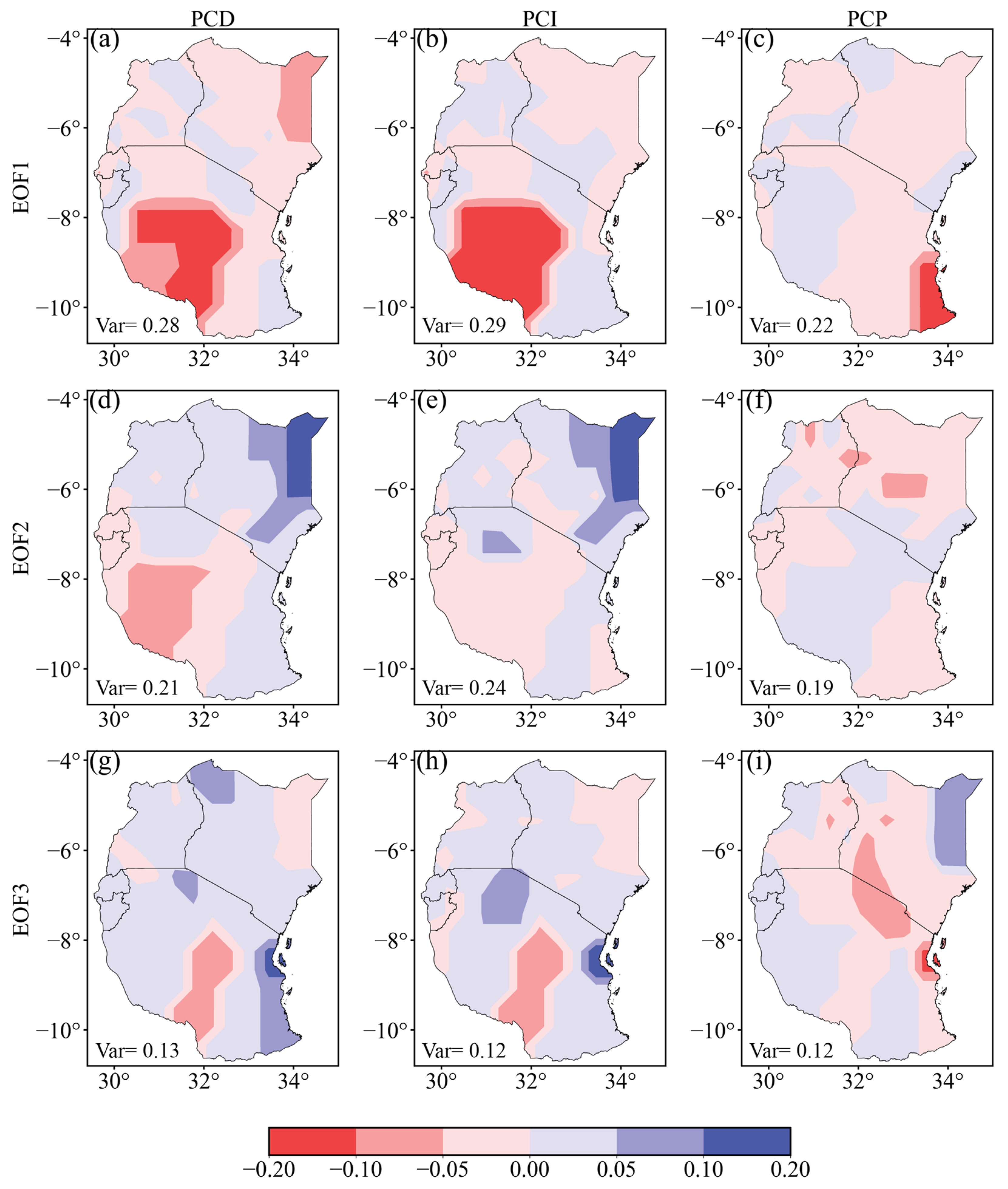
During the MAM season, the results for the EOF1 to EOF3 modes for the PCD showed 28%, 21%, and 13% loadings (Figure 4a,d,g). For the PCI, mode 1 showed the largest variance with 28% loadings, while modes 2 and 3 represented 24% and 12% variance (Table 4, Figure 4b,e,h). Meanwhile, the PCP depicted 22% loadings for mode 1 and 19% for mode 2, while the least loadings were noted in EOF mode 3 where it captured 12% variance (Table 4, Figure 4c,f,i). Accordingly, a homogeneous negative pattern was depicted over the whole region for the PCD, PCI, and PCP for the first mode, which signify reduced rainfall events. However, the second EOF model showed an apparent south–north dipole of negative-positive loadings for both the PCD and PCI over the region (Figure 4). Undoubtedly, the southern parts of Tanzania indicated a strong negative anomaly for the PCD and PCI during mode 1. This pattern showed reduced negative loadings for mode 2 and mode 3. On the contrary, positive loadings were demonstrated for EOF2, along the northeastern region of Kenya for the PCD and PCI values. The results denoted varying changes in the rainfall magnitude and period during the MAM season over the East Africa region. Moreover, the negative loadings in the PCP for all EOF analyses indicated how varying changes in the percentages of rainfall were associated with different rainy days. Considering the PC variability, most modes showed low variability with only one peak during 2000 that was recorded for both the PCD and PCI (Figure 5).

The amplitudes for the PCP for all modes showed negative anomalies during 1986, 1988, 1992, 1994, 2006, and most recently 2016 (Figure 5). In agreement with previous studies, the listed years showed that the region witnessed the occurrence of moderate to severe and extreme drought episodes over the study region [15,66,67,68]. Numerous studies detected the abrupt decline in MAM rainfall during 1992, and this pattern has sustained a similar tendency leading to extreme weather and climate anomalies such as drought events [16,28,69]. Particularly, the PCI, which represented the contribution of days of heavy rainfall to the total amount of rainfall over a certain period (i.e., 1 year), showed notable changes, which called for further analysis. Recent findings by Liebmann et al. [62] suggest that the decrease in MAM could be due to an increased zonal gradient in the SST between Indonesia and the central Pacific. This is in agreement with the observations by Funk et al. [70] on climatic conditions associated with drying trends in the western central Pacific and central Indian Ocean that reoccur during MAM. However, other studies (e.g., Indeje et al. [13]) showed that the long rainfall in MAM is dominated by local factors rather than the large-scale factors in regulating variability of rainfall. In contrast, the OND rainfall has been observed to increase and is projected to continue increasing to the end of the 21st century [16,17,69], mostly due to western Indian Ocean (WIO) warming [71].

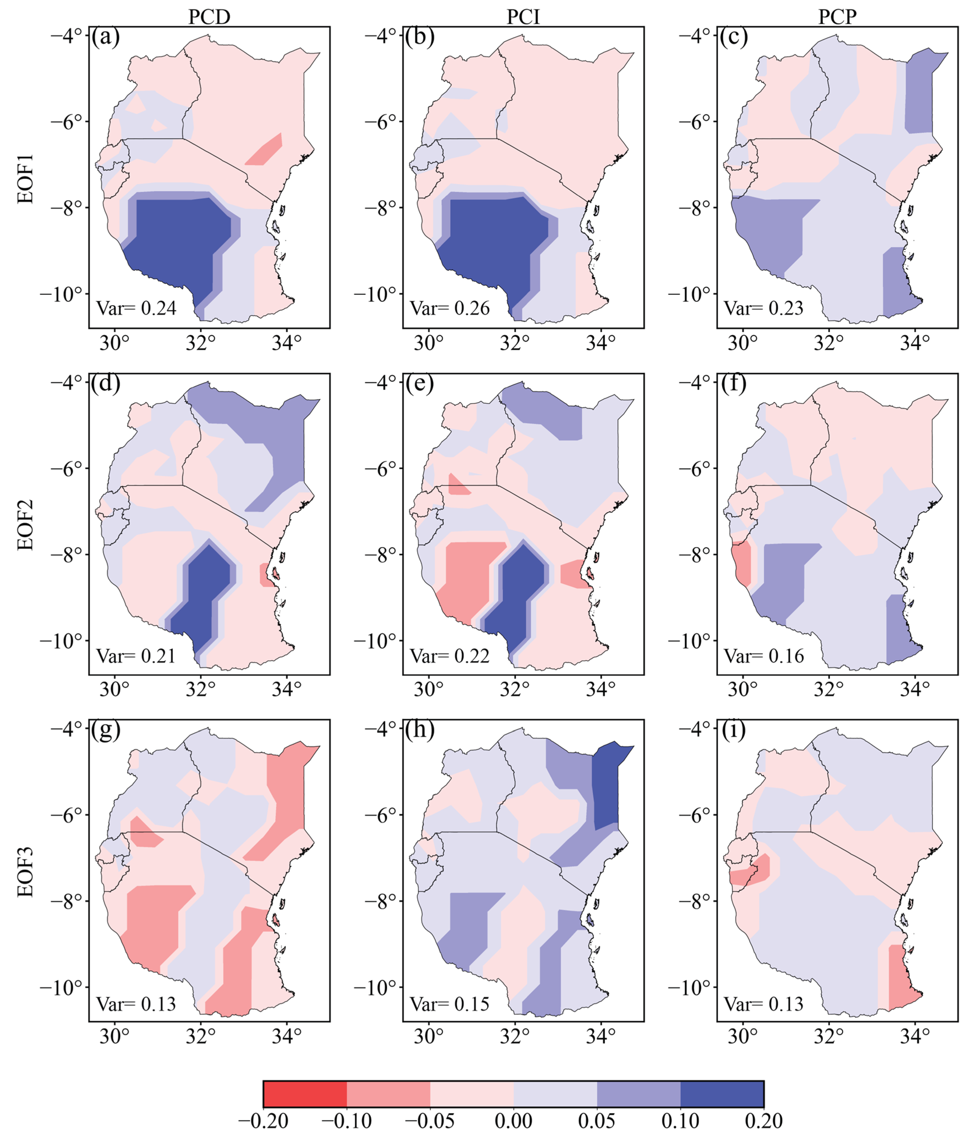
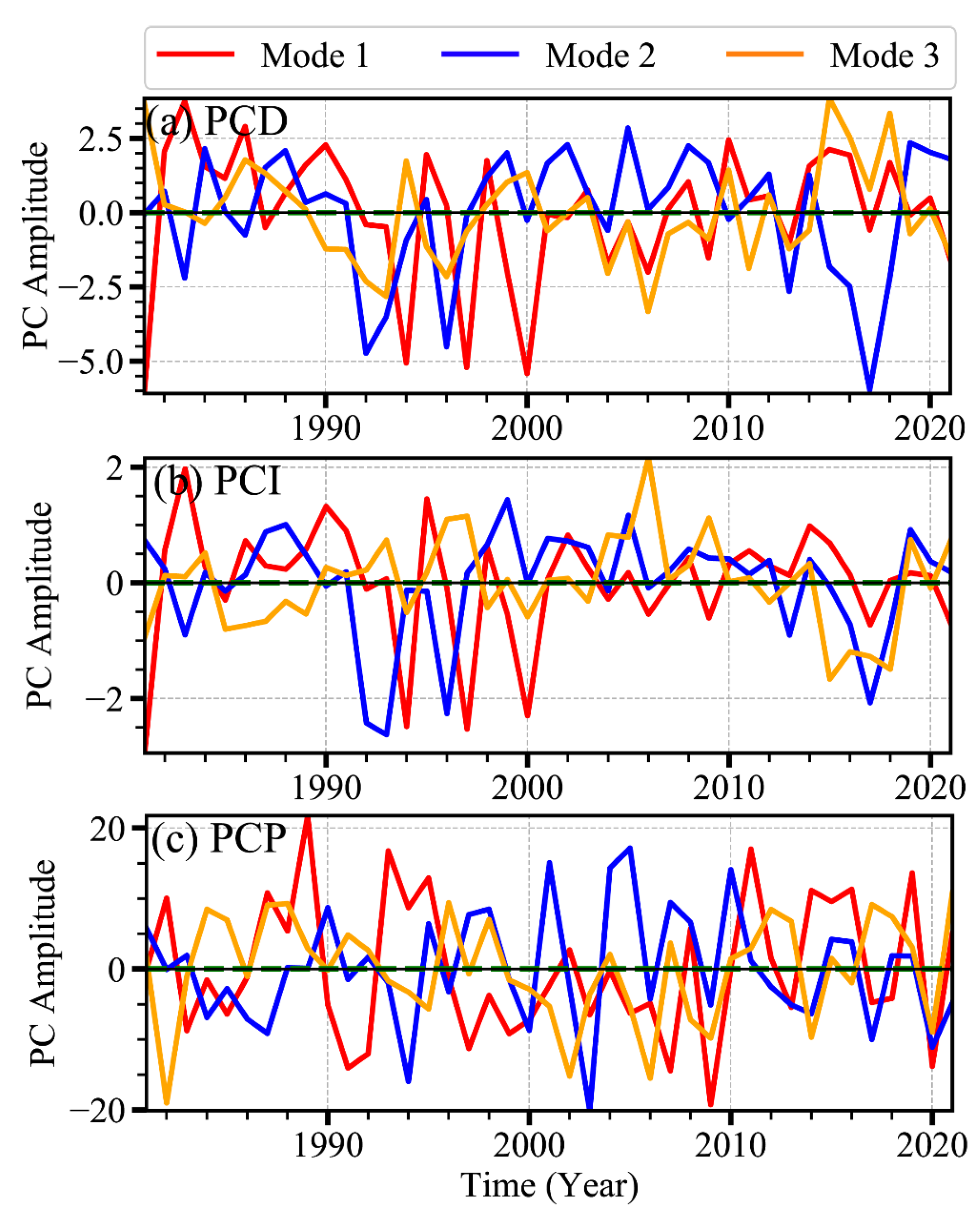
The observed spatial patterns in the EOF analysis for the PCD, PCI, and PCP during the OND season over East Africa during 1981 to 2021 are presented in Figure 6, Figure 7 and Figure 8 for the PC. These indices were useful in demonstrating the properties of the spatial and temporal characteristics of rainfall over East Africa during the study period. The results as illustrated in Figure 6 for spatial discrepancy and Figure 7 for temporal changes based on PC analysis highlighted varying changes in rainfall over the study region. Compared with the MAM season, the OND results showed a north–south dipole for EOF1 with 24% loadings for the PCD, 26% for the PCI, and 23% loadings for the PCP (Figure 6). Likewise, EOF2 and EOF3 for the PCD reflected 21% and 13% loadings, while those for the PCI denoted 22% and 15% loadings, respectively. The last index of PCP demonstrated the largest loadings in EOF1 (23%), while the subsequent second and third loadings were 16% and 13% (Table 4, Figure 6f,i). Overall, both the PCD and PCI showed similar patterns, with the southern Tanzania region depicting wet anomalies, while parts of Kenya and Uganda showed mainly dry anomalies. The observed high rainfall amount in the wet anomaly over southern Tanzania resulting in floods was related to the strong warm phase of ENSO [72]. The strong warming coupled with a convective zone over the western Indian Ocean and the EA region was also responsible for heavy rainfall over northern Tanzania in 2006 [71], consistent with the findings of [73]. It is interesting to note that the EOF3 for the PCI showed a homogenous negative anomaly covering the entire region. Similar patterns were captured in EOF3 for the PCP index (Figure 6i). Correspondingly, the years when the negative anomalies were observed for EOF3 based on the PC were 1982, 2002, 2006, and 2014 (Figure 7). This signified possible changes in the dynamics and thermodynamics factors controlling the rainfall over the region. For PCD and PCI under EOF1, which reflected the large variances, the anomalous wet (dry) years were 1983, 1995, and 2010 (1981, 1994, and 2000) (Figure 7). The findings indicated the failure of short rains, which could be attributed to the teleconnections of the SST changes with rainfall events in the region [65,72]. Recently, [32] also noted that the dry years as reflected in the PCD, PCI, and PCP could be attributed to the coupling of an easterly flow from the Indian Ocean and anomalous surface and mid-tropospheric flows from the northwestern and eastern Atlantic Ocean. On the other hand, the study further reported that the observed high rainfall amount as reflected in the positive PC variability for the listed indices was attributed to the strong warm phase of ENSO [32]. For example, in 1982, 1997, and 2006, wet conditions were linked to a positive phase of the IOD and a warm phase of the ENSO. The EOF1 for the PCD and PCI that reflected a wet anomaly over southern parts of Tanzania could be attributed to the strong warming coupled with a convective zone over the western Indian Ocean [72].

3.2. Spatial Trends of the PCD, PCI, and PCP

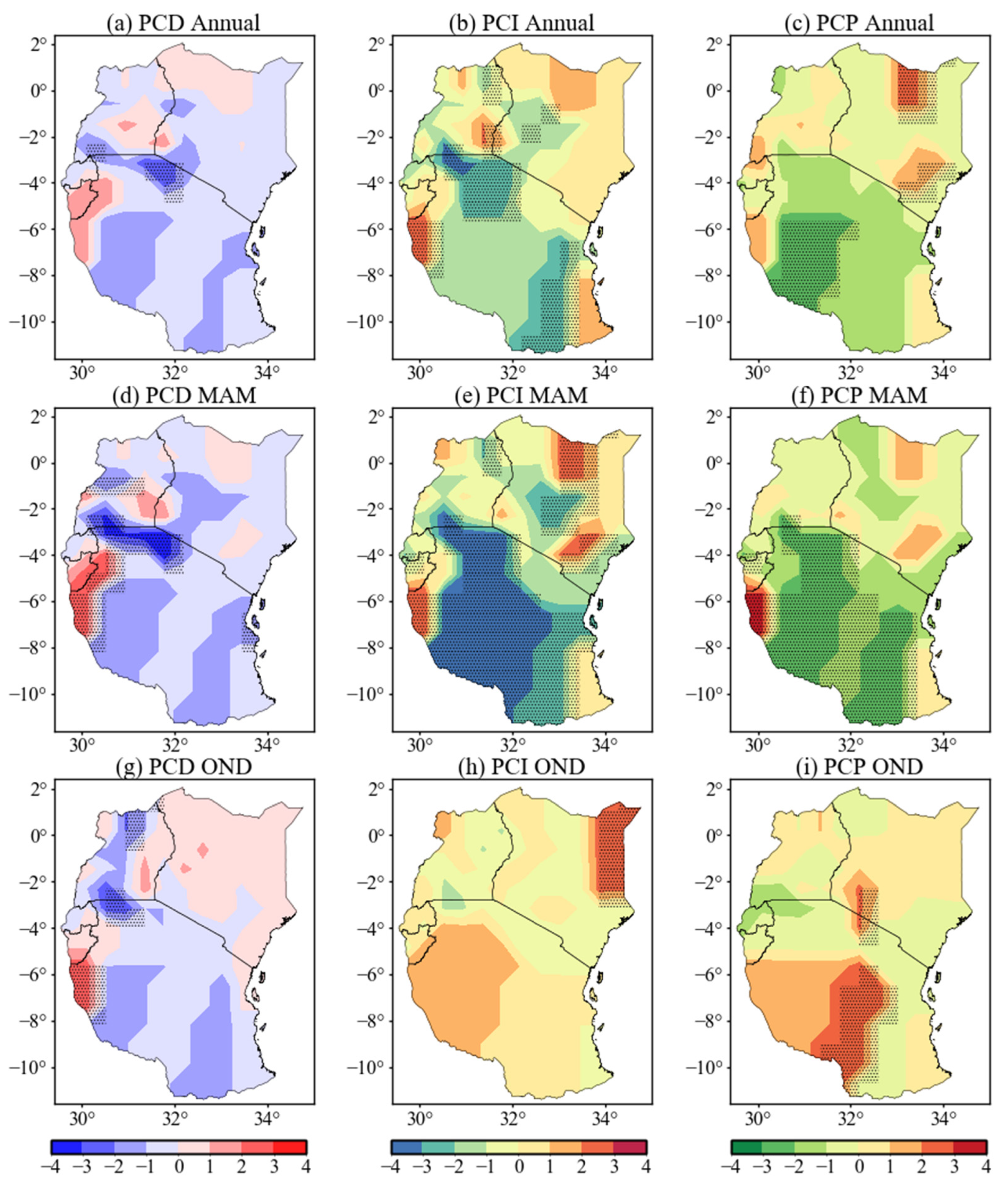
The modified Mann–Kendall statistical test and the Theil–Sen slope estimator were utilized to detect the possible trend changes in the PCD, PCI, and PCP and their respective magnitudes during the last 40 years over the EA region. Figure 8 shows the spatial patterns of the trends, while

Table 5. Values of modified Mann–Kendall test (M-MK) for annual time scale for the period 1981–2021.

No.	Station	PCD			PCI			PCP
		Slope	Z	P	Slope	Z	P	Slop	Z	P
1	Arua	0	1.88	0.06	0	−0.19	0.85	−0.01	−0.51	0.61
2	Buja	0	1.88	0.06	0	−0.19	0.85	−0.01	−0.51	0.61
3	Bukoba	−0.01	−3.26	0	−0.33	−3.87	0	−0.02	−1.26	0.21
4	Cankuzo	0	0.92	0.36	0.01	0.4	0.69	0.02	1.46	0.15
5	Dodoma	−0.01	−1.43	0.15	−0.56	−3.65	0	0.01	0.93	0.35
6	Eldoret	0	−1.6	0.11	−0.11	−1.9	0.06	0	0.15	0.88
7	Embu	0	0.95	0.34	−0.04	−0.71	0.48	0	0.56	0.58
8	Entebbe	0	−0.11	0.91	−0.02	−1.27	0.2	−0.01	−0.83	0.41
9	Garissa	0	0.84	0.4	0.08	0.83	0.41	0.03	2.39	0.02
10	Gisozi	0	−0.65	0.51	−0.01	−0.61	0.54	−0.01	−1.07	0.28
11	Gitega	0	1.88	0.06	0	−0.19	0.85	−0.01	−0.51	0.61
12	Gulu	0	1.49	0.14	0.01	0.44	0.66	0	0.03	0.97
13	Jinja	0	2.08	0.04	−0.01	−0.36	0.72	0	−0.12	0.91
14	Kabale	0	−1.22	0.22	−0.01	−0.91	0.36	0.01	0.58	0.56
15	Kampala	0	0.14	0.89	0	−0.33	0.74	−0.01	−0.95	0.34
16	Kasese	0	−1.65	0.1	0.01	0.42	0.67	0	−0.49	0.62
17	Kigali	0	−1.06	0.29	−0.2	−2.19	0.03	0.01	0.7	0.48
18	Kiige	0	0.99	0.32	0.01	0.39	0.69	0	0.43	0.67
19	Kilimanjaro	0	−0.3	0.76	−0.11	−1.34	0.18	−0.01	−0.7	0.49
20	Kisumu	0	1.55	0.12	0.05	1.54	0.12	0	0.28	0.78
21	Kitale	0	−1.31	0.19	−0.04	−1.69	0.09	−0.01	−0.44	0.66
22	Kitgum	0	−0.2	0.84	0	0.09	0.93	0.03	1.85	0.06
23	Lira	0	−2.02	0.04	−0.03	−2.27	0.02	−0.01	−0.43	0.67
24	Lodwar	0	0.26	0.8	−0.08	−0.6	0.55	0	0.03	0.97
25	Makindu	0	0.71	0.47	0.34	2.08	0.04	0	−0.19	0.85
26	Marsabit	0.01	1.85	0.06	0.27	2.23	0.03	0	−0.17	0.86
27	Masindi	0	−1.15	0.25	−0.02	−1.25	0.21	0	0.09	0.93
28	Mbarara	0	0.9	0.37	−0.03	−1.51	0.13	0.01	0.91	0.36
29	Meru	0	0.44	0.66	−0.01	−0.11	0.91	−0.01	−0.48	0.63
30	Morogoro	−0.01	−2.83	0	−0.24	−2.56	0.01	0.01	0.79	0.43
31	Musasa	0	2.41	0.02	0.04	2.76	0.01	0.02	1.31	0.19
32	Musoma	−0.01	−2.93	0	−0.27	−3.8	0	0	−0.04	0.96
33	Muyinga	0	0.83	0.4	−0.01	−0.36	0.72	−0.01	−0.53	0.6
34	Mwalimu	0	1.05	0.3	0.04	0.58	0.56	0	0.5	0.9
35	Mwanza	−0.01	−2.9	0	−0.24	−3.24	0	0.01	1.2	0.23
36	Nairobi_Jk	0	−0.47	0.64	−0.09	−1.63	0.1	0.01	0.94	0.35
37	Nakuru	0	−1.31	0.19	−0.02	−0.61	0.54	−0.01	−0.78	0.44
38	Namulonge	0	0.18	0.86	0	0.26	0.8	0	0.25	0.8
39	Nyeri	0	−1.25	0.21	−0.21	−2.58	0.01	−0.01	−0.58	0.56
40	Nymanza	0	0.15	0.88	−0.01	−0.56	0.57	0	−0.17	0.87
41	Serere	0	−1.11	0.27	−0.02	−1.24	0.22	0.02	1.55	0.12
42	Soroti	0	0.05	0.96	−0.01	−0.53	0.6	−0.02	−1.22	0.22
43	Tabora	−0.01	−1.84	0.07	−0.49	−3.79	0	0.01	1.43	0.15
44	Tororo	0	0.07	0.95	0	0.15	0.88	0	0.5	0.9
45	Voi	0	0.3	0.76	−0.05	−1.17	0.24	−0.01	−0.63	0.53
46	Zanzibar	0	−1.08	0.28	−0.2	−2.69	0.01	0.01	0.67	0.51

,

Table 6. Values of M-MK at MAM time scale for the period 1981–2021.

No.	Station	PCD			PCI			PCP
		Slope	Z	P	Slope	Z	P	Slop	Z	P
1	Arua	0	0.93	0.35	0.03	1.64	0.1	0.01	2.12	0.03
2	Buja	0	0.93	0.35	0.03	1.64	0.1	0.01	2.12	0.03
3	Bukoba	0	−1.27	0.2	−0.1	−3.27	0	−0.03	−2.83	0
4	Cankuzo	0	1.56	0.12	0.04	2.45	0.01	0	0.87	0.39
5	Dodoma	0	−0.33	0.74	−0.03	−0.71	0.48	0	−0.65	0.51
6	Eldoret	0	−0.75	0.45	−0.05	−1.12	0.26	0.02	1.28	0.2
7	Embu	0	0.91	0.36	0.03	0.79	0.43	0	0.4	0.9
8	Entebbe	0	0.3	0.76	0	−0.67	0.5	0	−0.83	0.41
9	Garissa	0	−0.47	0.64	−0.03	−0.68	0.5	0.01	0.93	0.35
10	Gisozi	0	1.39	0.16	0.01	1.12	0.26	0	0.84	0.4
11	Gitega	0	0.93	0.35	0.03	1.64	0.1	0.01	2.12	0.03
12	Gulu	0	0.16	0.87	0	0.19	0.85	−0.01	−2.14	0.03
13	Jinja	0	0.71	0.48	0.01	1.29	0.2	0.01	1.46	0.15
14	Kabale	0	−0.53	0.6	0	−0.15	0.88	0	0.6	0.9
15	Kampala	0	−0.62	0.54	0	−0.15	0.88	0.01	2.88	0
16	Kasese	0	−0.38	0.7	0.02	1.62	0.11	0	0.7	0.49
17	Kigali	0	−1.13	0.26	−0.05	−0.96	0.34	−0.01	−0.46	0.65
18	Kiige	0	0.56	0.57	0.01	0.62	0.54	0.01	1.99	0.05
19	Kilimanjaro	0	−0.02	0.98	−0.02	−0.35	0.73	−0.01	−0.63	0.53
20	Kisumu	0	1.89	0.06	0.03	1.77	0.08	0	−0.22	0.82
21	Kitale	0	−1.72	0.09	−0.03	−1.39	0.16	0	0.26	0.8
22	Kitgum	0	−0.01	0.99	0	−0.4	0.69	0	−0.54	0.59
23	Lira	0	−0.75	0.45	−0.01	−0.73	0.47	−0.01	−1.19	0.23
24	Lodwar	0	0.23	0.82	−0.01	−0.13	0.9	0	0.41	0.68
25	Makindu	0	−0.1	0.92	0.01	0.08	0.94	0	−0.14	0.89
26	Marsabit	0	0.6	0.55	0.07	0.65	0.52	0	0.24	0.81
27	Masindi	0	−1.05	0.3	−0.02	−1.98	0.05	−0.01	−1.24	0.22
28	Mbarara	0	−2.01	0.04	−0.03	−2.06	0.04	−0.01	−1.02	0.31
29	Meru	0	0.07	0.95	0	−0.01	0.99	0	−0.29	0.77
30	Morogoro	0	−1.03	0.3	−0.05	−1.34	0.18	−0.02	−1.81	0.07
31	Musasa	0	1.19	0.23	0.04	2.25	0.02	0.01	2.53	0.01
32	Musoma	−0.01	−2.89	0	−0.14	−3.96	0	−0.01	−1	0.32
33	Muyinga	0	0.99	0.32	0.01	0.83	0.41	0	0.26	0.8
34	Mwalimu	0	−0.34	0.74	−0.02	−0.45	0.65	0	−0.27	0.79
35	Mwanza	0	−0.17	0.87	−0.03	−0.75	0.45	0	−0.35	0.73
36	Nairobi_Jk	0	−0.97	0.33	0	−0.16	0.88	0	0.38	0.7
37	Nakuru	0	−1.43	0.15	−0.04	−1.65	0.1	0	−0.15	0.88
38	Namulonge	0	1.38	0.17	0	0.57	0.57	0	−1.16	0.25
39	Nyeri	0	−0.75	0.46	−0.04	−1.35	0.18	0	0.59	0.56
40	Nymanza	0	1.16	0.25	0.01	1.04	0.3	0	0.45	0.65
41	Serere	0	−0.83	0.41	−0.01	−1	0.32	0	−0.69	0.49
42	Soroti	0	0.8	0.42	0.01	0.36	0.72	0	0.71	0.48
43	Tabora	0	−1.91	0.06	−0.1	−1.95	0.05	−0.01	−1.07	0.28
44	Tororo	0	0.19	0.85	0.01	0.65	0.51	0	−0.81	0.42
45	Voi	0	−0.34	0.74	−0.04	−0.87	0.38	0	0.49	0.62
46	Zanzibar	0	−1.54	0.12	−0.13	−1.97	0.05	0	0.1	0.92

and

Table 7. Values of M-MK at OND time scale for the period 1981–2021.

No.	Station	PCD			PCI			PCP
		Slope	Z	P	Slope	Z	P	Slope	Z	P
1	Arua	0	0.64	0.52	0.01	0.73	0.47	0	0.55	0.58
2	Buja	0	0.64	0.52	0.01	0.73	0.47	0	0.55	0.58
3	Bukoba	0	−1.72	0.09	−0.1	−2.43	0.02	−0.02	−1.63	0.1
4	Cankuzo	0	−0.93	0.35	−0.01	−1.29	0.2	0	−0.26	0.8
5	Dodoma	0	−1.88	0.06	−0.11	−1.99	0.05	0.01	2.52	0.01
6	Eldoret	0	−1.01	0.31	−0.12	−1.28	0.2	0.01	0.96	0.34
7	Embu	0	−0.16	0.87	−0.01	−0.31	0.75	0	−0.34	0.74
8	Entebbe	0	0.59	0.56	0	0.42	0.68	0	0.49	0.62
9	Garissa	0	−0.08	0.94	0	0.5	0.9	0	0.33	0.74
10	Gisozi	0	−0.82	0.41	0.01	0.87	0.38	0	−0.38	0.7
11	Gitega	0	0.64	0.52	0.01	0.73	0.47	0	0.55	0.58
12	Gulu	0	−0.35	0.73	−0.01	−0.4	0.69	0	−0.01	0.99
13	Jinja	0	0.09	0.93	0	0.4	0.9	0	−0.07	0.95
14	Kabale	0	1.52	0.13	−0.01	−0.47	0.64	−0.01	−1.39	0.16
15	Kampala	0	0.34	0.74	0	−0.44	0.66	0	−0.84	0.4
16	Kasese	0	0.29	0.77	0.01	0.34	0.74	0	0.62	0.54
17	Kigali	0	−1.29	0.2	−0.08	−2.37	0.02	−0.03	−1.87	0.06
18	Kiige	0	−1.91	0.06	−0.03	−1.38	0.17	0	0.5	0.9
19	Kilimanjaro	0	−1.28	0.2	−0.08	−1.31	0.19	0	−0.35	0.73
20	Kisumu	0	0.85	0.39	0.02	1.35	0.18	0.01	0.75	0.45
21	Kitale	0	−0.6	0.55	−0.03	−0.79	0.43	0.01	0.76	0.44
22	Kitgum	0	−0.4	0.69	−0.05	−1.12	0.26	−0.02	−2.2	0.03
23	Lira	0	0.35	0.73	−0.01	−0.22	0.82	0.01	1.08	0.28
24	Lodwar	0	−0.97	0.33	−0.05	−1.11	0.27	0	−0.41	0.68
25	Makindu	0.01	1.99	0.05	0.14	1.72	0.09	0	−0.34	0.73
26	Marsabit	0.01	2.02	0.04	0.09	1.3	0.19	0	0.4	0.69
27	Masindi	0	−0.85	0.39	0	−0.3	0.76	0	0.31	0.75
28	Mbarara	0	1.35	0.18	0	0.03	0.97	−0.01	−1.44	0.15
29	Meru	0	0.7	0.49	0.01	0.37	0.71	0	0.21	0.83
30	Morogoro	0	−1.85	0.06	−0.12	−2.65	0.01	0	−0.36	0.72
31	Musasa	0	1.93	0.05	0.04	3.01	0	0.01	1.59	0.11
32	Musoma	0	−1.59	0.11	−0.08	−2.29	0.02	−0.01	−0.87	0.38
33	Muyinga	0	0	1	−0.01	−0.74	0.46	0	0.02	0.98
34	Mwalimu	0	0.64	0.52	0.01	0.33	0.74	0.01	0.57	0.57
35	Mwanza	0	−1.15	0.25	−0.07	−2.13	0.03	0	−0.38	0.71
36	Nairobi_Jk	0	0.09	0.93	−0.01	−0.55	0.58	0	0.44	0.66
37	Nakuru	0	−0.53	0.6	0	0.04	0.96	0.01	2.21	0.03
38	Namulonge	0	1.1	0.27	−0.01	−0.66	0.51	0	−0.92	0.36
39	Nyeri	0	−0.66	0.51	−0.03	−1.2	0.23	0.01	0.97	0.33
40	Nymanza	0	0.38	0.7	0	0.1	0.92	0	−0.48	0.63
41	Serere	0	−0.52	0.61	−0.01	−0.24	0.81	0	0.18	0.86
42	Soroti	0	0.26	0.8	−0.01	−0.37	0.71	0	−0.8	0.42
43	Tabora	−0.01	−2.72	0.01	−0.17	−2.71	0.01	0.02	1.44	0.15
44	Tororo	0	−0.99	0.32	0	−0.31	0.75	0	−0.35	0.73
45	Voi	0	−0.32	0.75	−0.04	−1.25	0.21	0	−0.18	0.86
46	Zanzibar	0	−1.61	0.11	−0.09	−1.83	0.07	0	−0.46	0.65

enumerate the statistical values of the trend change both annually and for the seasons of MAM and OND, respectively. It is evident that the declining trends in the PCD were noted annually and during the MAM season over EA, while the opposite tendency was noted for the OND season where positive increasing trends in the PCD were observed (Figure 9a,d,g). Whereas the large spatial variance showed declining trends over EA for the PCD values, the regions adjacent to Lake Victoria in Uganda and Lake Tanganyika in Tanzania showed increasing trends in the PCD during the annual and seasonal time scales. This showed that the regions experienced convective rainfall throughout the year and during the rainfall season as a result of the large water bodies. A similar situation was noted along northern Kenya where Lake Turkana was situated with PCD values annually and for MAM showing positive tendencies, despite the negative patterns over other regions (Figure 8a,d). During the OND season, the PCD depicted declining trends in large areas in the Tanzania region and some parts of Uganda, while most parts of Kenya showed an increasing trend in the PCD (Figure 8g). Meanwhile, a strong signal of positive spatial variance for the PCI was observed over the whole region with a significant change recorded over the northeastern sides of Kenya with a Z-value of 4/year.

On the other hand, during the MAM season, significant declining trends were observed over most parts of Tanzania and the southern parts of the Uganda region for PCI Z-values ranging between −3.96 and −3.27/year (Table 6 and Table 7). Interestingly, despite the noteworthy negative trends in the PCI over most parts of Tanzania during the MAM season, the far western tip close to the Burundi region (around Lake Tanganyika) depicted positive PCI values, an affirmation of the impact of the convective rainfall event that contributes to sustained rainfall throughout the months. For the OND season, the study observed an increasing trend in the spatial distribution of the PCI during the study period, with significant increases noted along the northeastern parts of Kenya, the northwestern tip of Uganda, and the southwestern parts of Tanzania, respectively (Figure 8h).

The study estimated the spatial trends in the PCP annually and during the MAM/OND seasons. Figure 8c,f,i shows the historical trends during the last four decades with the statistical values of the slope, Z-values, and their respective significances listed in Table 5, Table 6 and Table 7. The results showed that the region experienced increasing trends in the PCP during the OND season, while general negative trends were noted for the MAM and annual time scales, except for a few isolated parts that depicted positive increases. To illustrate, the mean annual PCP showed increases over Kenya and Uganda, similar to other indices, while the Tanzania region demonstrated negative declining trends. On the other hand, the regions close to water bodies, such as the Tana River Basin in Kenya, Lake Tanganyika in Tanzania, and around Lake Victoria, mainly highlighted opposite positive trends during the study period. This showed that the degree of rainfall concentration, the period, and the distribution were largely influenced by the local geomorphology and land use factors (i.e., land cover properties, complex elevation, large water bodies, and soil moisture) and large-scale teleconnection factors [74].

Generally, a positive tendency was observed during the OND season for the PCD, PCI, and PCP across the region, while the MAM season demonstrated negative trends in the PCD, PCI, and PCP, especially for regions below the equator (Figure 8d–f). These findings highlighted the recent changes in rainfall patterns over the EA region since 1992. Historically, the MAM season is predominantly a longer season with rainfall distribution, concentration, and period lasting for three months and experienced over the region and is regarded as “long-rains” [16,28,75]. This is mainly due to the seasonal migration of the ITCZ [29] that brings moist convergence of westerlies. However, since 1992, numerous studies have reported a change in the trend with abrupt declining tendencies reported in 1992 [16,70,76,77]. The change in the trends has been attributed to the net impact of El Nino on the MAM season that tends to be insignificant due to anomalies switching sign in the middle of season, from positive in March of the post El Nino year to a negative shift during May and close to zero in April [64]. Moreover, other studies (i.e., [62,78,79]) reported that the abrupt change in MAM rainfall could be attributed to a weak ENSO signal. They demonstrated that La Nina could amplify either the increase or decrease in MAM rainfall over the study region, depending on the features of the episode. More details on the characteristics of the ENSO signal can be obtained from an extensive review literature of EA rainfall variability by [72]. Meanwhile, the observed positive trends in the OND season for the PCD, PCI, and PCP could be linked to the recent changes in the SST of the Indian and Pacific Oceans. Many studies have reported that the OND season, also referred to as “short rains”, is mainly linked to the Walker circulation cell over the Indian Ocean [25,71,72]. The variability of the Walker circulation is strongly connected to the Indian Ocean Dipole, which is associated with pronounced rainfall events over the last few years over the region. In addition to the SST conditions of the Indian Ocean that strongly modulate the OND rainfall, it should be noted that changes in trends for the SST over the Pacific and Atlantic also contribute to the increased rainfall during OND, evidenced by positive increase in the PCD, PCI, and PCP [73,74,75].

Overall, the regions where positive/negative trends were detected should be paid close attention due to the roles that they play in supporting livelihoods. Using these indices can provide an overview of recent changes in the distribution, the concentration, and the period of change for adequate policy changes. Many other existing studies across different regions have noted varying changes in trends based on the Mann–Kendall test for either the PCI, PCD, and PCP or one of them [1,10,31].

3.3. The Periodical Characteristics of Rainfall PCD, PCI, and PCP

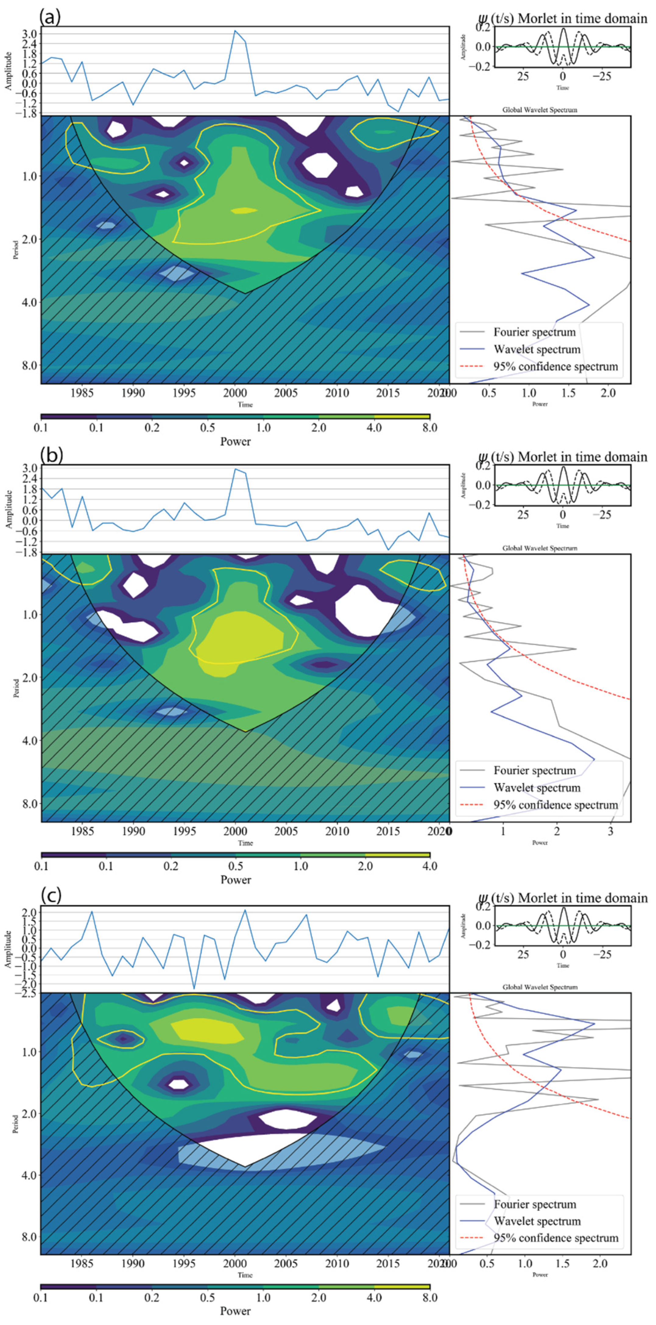
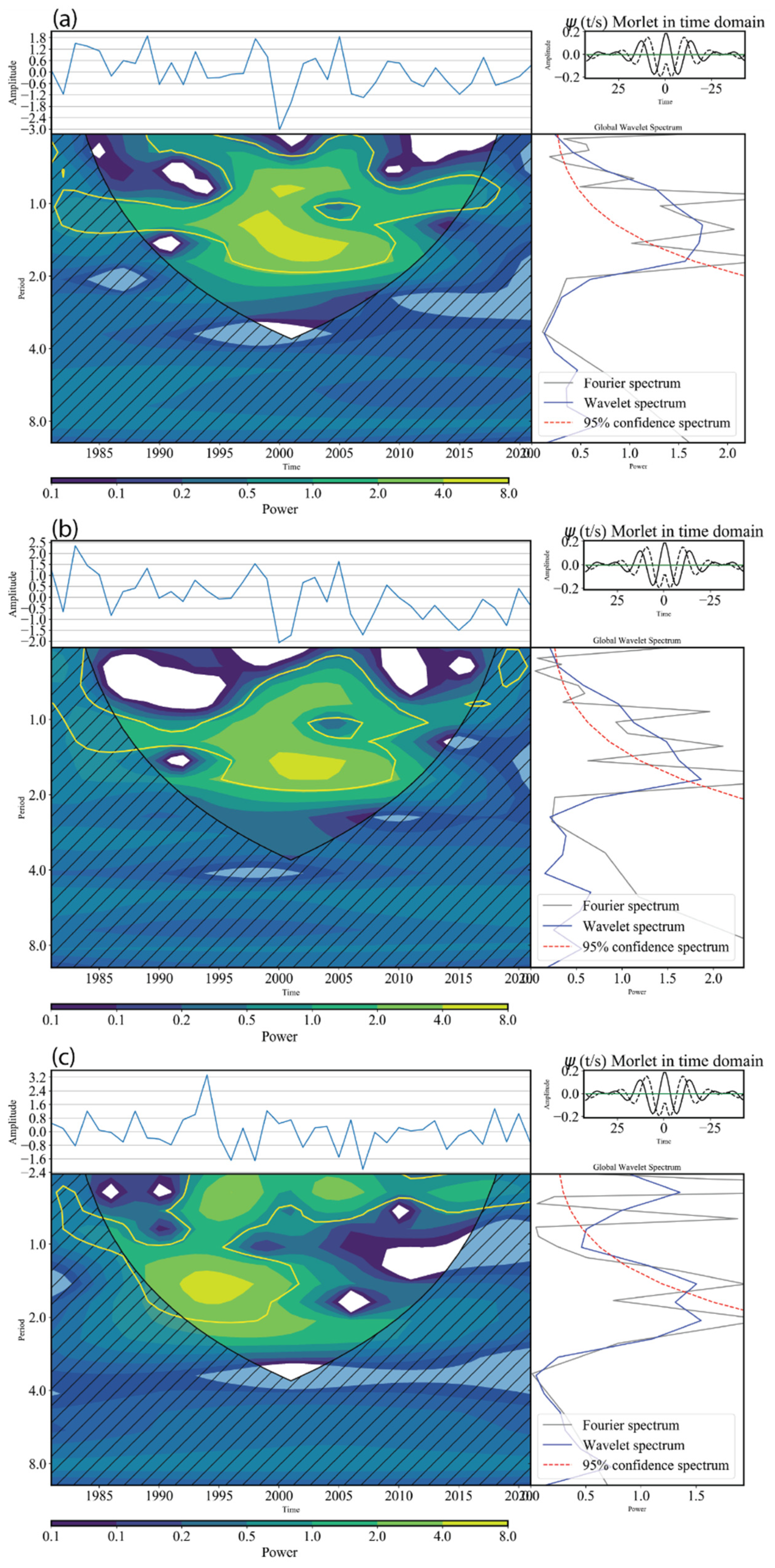
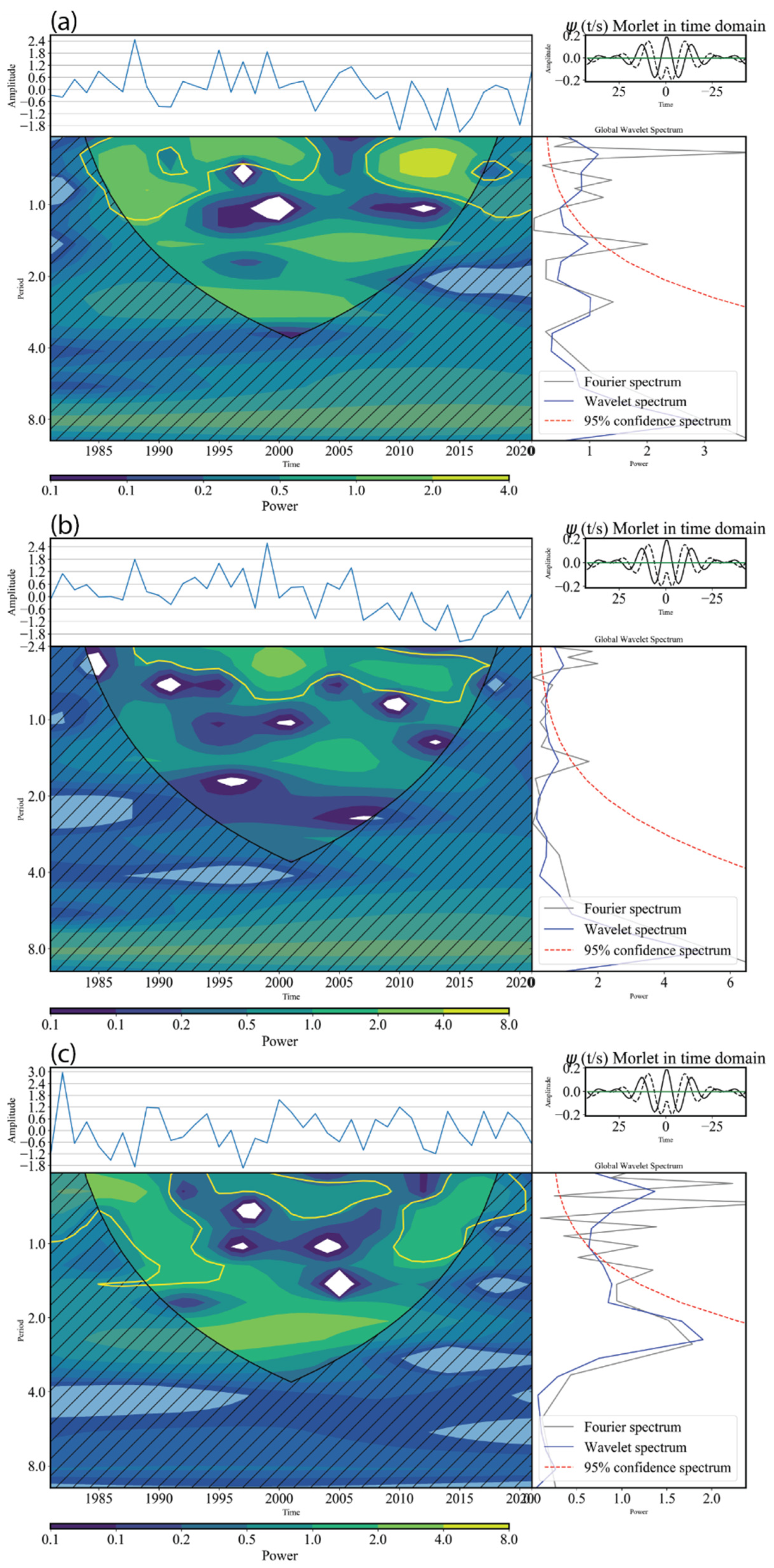
Further analyses to characterize the rainfall cycle and possible return period, considering the indices of the PCD, PCI, and PCP, were conducted over the study region using wavelet analysis. Figure 9 presents the wavelet power spectrum of the annual PCD, PCI, and PCP time series from the area-averaged stations in EA during 1981–2021. The rainfall indices’ frequency modes of variability were detected using the continuous wavelet transform due to its localization in time and frequency, which caused it to be a convenient means of identifying rainfall spatial structures [80,81,82]. The time series of the PCD is presented in Figure 9a, and the corresponding wavelet power spectrum (WPS) of the monthly rainfall PCD is demonstrated in the same diagram. Meanwhile, the dark contour lines in the WPS indicate areas where the confidence level in relation to the red noise background spectrum was more than 95%, while the “cone of influence” delineated by the narrow solid curve is where edge effects were taken into account. Similar analyses were conducted for the MAM (Figure 10) and OND seasons (Figure 11). Overall, the results for the annual PCD revealed noteworthy multiple bands of variability of typical periodicity as enclosed by the contours greater than the 95% confidence level for the annual mean PCD, PCI, and PCP events. The time series for the PCI and PCD showed higher variability during the year 2000, while much variability was shown in the PCP for the annual period. During the MAM and OND seasons, a 1-year band as a dominant period of variability was observed in all the indices. It is worth noting that the power spectrum at a 1.0–2.0-year cycle showed multiple occurrences of substantial periodicity that were contained within the borders of the greater than 95% confidence level. The wettest years were 1996–1997, 2001–2002, and 2010, and these were the years where the signals were most clearly localized. Meanwhile, the global wavelet spectrum’s annual periodicity indicated multiple notable peaks above the 95% confidence level for the MAM season, while one notable peak was depicted for the OND season in the PCD. Overall, the results of the wavelet transform revealed the completion of the time scale representation of the localized frequency information and transient events occurring at varying time scales as depicted for the PCD, PCI, and PCP indices over East Africa.

4. Conclusions

In this study, we explored the observed changes in rainfall concentration over East Africa during the last 40 years (1981–2021), in a bid to quantify the spatial and temporal changes in rainfall that are useful for stakeholders in agriculture, hydrology, water management resources, and flood disaster management. The study employed suitable matrices of PCI, PCD, and PCP to analyze the monthly distribution of rainfall over the study region annually and during the MAM and OND seasons. The PCI was generally used for quantifying the distribution of the rainfall pattern and the calculation of seasonal changes, while the PCD aided the investigation of the concentration characteristics of rainfall. Meanwhile, the PCP represented the degree to which the total annual rainfall was concentrated over 12 months. In our study, we employed various techniques such as EOF analyses for detecting spatiotemporal variances, modified Mann–Kendall and the Theil–Sen slope estimator for trend and magnitude changes, and continuous wavelet transforms for exploring the frequency modes of variability for the indices. A summary of our findings is itemized as follows:

Spatiotemporal changes based on the EOF show mode 1 was predominantly depicting positive loadings over most parts of the region for the PCD, with only the western region of Uganda showing negative loadings. Moreover, several peaks during 1984, 1992, 1996, 1999, 2004, 2005, 2008, 2000, and 2014, denoting anomalous wet/dry conditions when the degree of rainfall concentration during the study period was below or above the normal thresholds, were noted. Overall, the positive changes in PCI were predominant over the Tanzania region during mode 1, while mode 2 illustrated overall positive loadings over the entire region. The spatial variance as demonstrated in the EOF analysis highlighted the observed changes in rainfall concentration over the region, with locations such as western Uganda, Rwanda, and Burundi calling for an urgent intervention for water resources.

The trend analysis for rainfall concentration over EA indicated declining trends in the PCD annually and during the MAM season over EA, while the opposite tendency was noted for the OND season where positive increasing trends in the PCD were observed. The regions adjacent to Lake Victoria in Uganda and Lake Tanganyika in Tanzania showed increasing trends in the PCD during annual and seasonal time scales.

Last, the study employed a wavelet transform to detect the temporal extent of the indices, as well as to determine their frequencies over EA during annual and seasonal time scales. The findings for the annual time scale revealed noteworthy multiple bands of variability of typical periodicity as enclosed by the contours with greater than 95% confidence levels for the annual mean PCD, PCI, and PCP events. The time series for PCI and PCD showed higher variability during the year 2000, while much more variability was shown in the PCP for the annual period. During the MAM and OND seasons, a 1-year band as a dominant period of variability was observed in all the indices. It is worth noting that the power spectrum at the 1.0–2.0/year cycle showed multiple occurrences of substantial periodicity that were contained within the borders of the greater than 95% confidence level.

Overall, the findings of the present study highlighted regions where detectable reductions in precipitation concentration were more pronounced, and possible trends were highlighted. Moreover, the periodicity characteristics showed pronounced interannual variability, which is the basis for further investigation of the underlying mechanisms.

The detailed mechanisms that affect the change of precipitation characteristics need further research. Future research will focus on the physical mechanisms that underlie the spatiotemporal distributions of the precipitation concentration indices, quantitative analyses of the contributions of atmospheric circulation factors to precipitation change, and simulations of future variations in precipitation concentrations based on regional climate models. Further studies must be conducted to fully understand the responses of water systems to climate change and assess the relationships between precipitation anomalies and precipitation variations over East Africa.

References

- Li, Q.; Yang, M.; Wan, G.; Wang, X. Spatial and temporal precipitation variability in the source region of the Yellow River. Environ. Earth Sci. 2016, 75, 594. [Google Scholar] [CrossRef]
- Apaydin, H.; Erpul, G.; Bayramin, I.; Gabriels, D. Evaluation of indices for characterizing the distribution and concentration of precipitation: A case for the region of Southeastern Anatolia Project, Turkey. J. Hydrol. 2006, 328, 726–732. [Google Scholar] [CrossRef]
- Gabriels, D. Assessing the Modified Fournier Index and the Precipitation Concentration Index for Some European Countries. In Soil Erosion in Europe; John Wiley & Sons, Ltd.: Chichester, UK, 2006; pp. 675–684. [Google Scholar]
- Teixeira, J.C.; Carvalho, A.C.; Carvalho, M.J.; Luna, T.; Rocha, A. Sensitivity of the WRF model to the lower boundary in an extreme precipitation event—Madeira island case study. Nat. Hazards Earth Syst. Sci. 2014, 14, 2009–2025. [Google Scholar] [CrossRef]
- Oliver, J.E. Monthly Precipitation Distribution: A Comparative Index. Prof. Geogr. 1980, 32, 300–309. [Google Scholar] [CrossRef]
- De Luis, M.; González-Hidalgo, J.C.; Raventós, J.; Sánchez, J.R.; Cortina, J. Distribución Espacial de la Concentración y Agresividad de la lluvia en el territorio de la Comunidad Valenciana. Cuaternario Geomorfol. 1997, 11, 33–44. [Google Scholar]
- Zhang, Y.; Qian, L. Annual distribution features of precipitation in China and their interannual variations. Acta Meteorol. Sin. 2003, 2, 146–163. [Google Scholar]
- Benhamrouche, A.; Boucherf, D.; Hamadache, R.; Bendahmane, L.; Martin-Vide, J.; Teixeira Nery, J. Spatial distribution of the daily precipitation concentration index in Algeria. Nat. Hazards Earth Syst. Sci. 2015, 15, 617–625. [Google Scholar] [CrossRef]
- Bessaklia, H.; Ghenim, A.N.; Megnounif, A.; Martin-Vide, J. Spatial variability of concentration and aggressiveness of precipitation in North-East of Algeria. J. Water Land Dev. 2018, 36, 3–15. [Google Scholar] [CrossRef]
- Njouenwet, I.; Tchotchou, L.A.D.; Ayugi, B.O.; Guenang, G.M.; Vondou, D.A.; Nouayou, R. Spatiotemporal Variability, Trends, and Potential Impacts of Extreme Rainfall Events in the Sudano-Sahelian Region of Cameroon. Atmosphere 2022, 13, 1599. [Google Scholar] [CrossRef]
- Assamnew, A.D.; Tsidu, G.M. Spatiotemporal characteristics of current and projected rainfalls over East Africa: Insights from precipitation concentration and standardized precipitation indices. Res. Sq. 2022. [Google Scholar] [CrossRef]
- Azioune, R.; Benhamrouche, A.; Tatar, H.; Martin-Vide, J.; Pham, Q.B. Analysis of daily rainfall concentration in northeastern Algeria 1980–2012. Theor. Appl. Climatol. 2023, 153, 1361–1370. [Google Scholar] [CrossRef]
- Indeje, M.; Semazzi, F.H.M.; Ogallo, L.J. ENSO signals in East African rainfall seasons. Int. J. Climatol. 2000, 20, 19–46. [Google Scholar] [CrossRef]
- Kebacho, L.L.; Chen, H. The dominant modes of the long rains interannual variability over Tanzania and their oceanic drivers. Int. J. Climatol. 2022, 42, 5273–5292. [Google Scholar] [CrossRef]
- Nicholson, S.E. Dryland Climatology; Cambridge University Press: Cambridge, UK, 2011; 516p. [Google Scholar] [CrossRef]
- Palmer, P.I.; Wainwright, C.M.; Dong, B.; Maidment, R.I.; Wheeler, K.G.; Gedney, N.; Hickman, J.E.; Madani, N.; Folwell, S.S.; Abdo, G.; et al. Drivers and impacts of Eastern African rainfall variability. Nat. Rev. Earth Environ. 2023, 4, 254–270. [Google Scholar] [CrossRef]
- Endris, H.S.; Omondi, P.; Jain, S.; Lennard, C.; Hewitson, B.; Chang’a, L.; Awange, J.L.; Dosio, A.; Ketiem, P.; Nikulin, G.; et al. Assessment of the performance of CORDEX regional climate models in simulating East African rainfall. J. Clim. 2013, 26, 8453–8475. [Google Scholar] [CrossRef]
- Shongwe, M.E.; van Oldenborgh, G.J.; van den Hurk, B.; van Aalst, M. Projected changes in mean and extreme precipitation in Africa under global warming—Part II: East Africa. J. Clim. 2011, 24, 3718–3733. [Google Scholar] [CrossRef]
- Kilavi, M.; MacLeod, D.; Ambani, M.; Robbins, J.; Dankers, R.; Graham, R.; Helen, T.; Salih, A.A.M.; Todd, M.C. Extreme rainfall and flooding over Central Kenya Including Nairobi City during the long-rains season 2018: Causes, predictability, and potential for early warning and actions. Atmosphere 2018, 9, 472. [Google Scholar] [CrossRef]
- Gebrechorkos, S.H.; Hülsmann, S.; Bernhofer, C. Changes in temperature and precipitation extremes in Ethiopia, Kenya, and Tanzania. Int. J. Climatol. 2019, 39, 18–30. [Google Scholar] [CrossRef]
- Finney, D.L.; Marsham, J.H.; Rowell, D.P.; Kendon, E.J.; Tucker, S.O.; Stratton, R.A.; Jackson, L.S. Effects of explicit convection on future projections of mesoscale circulations, rainfall, and rainfall extremes over eastern Africa. J. Clim. 2020, 33, 2701–2718. [Google Scholar] [CrossRef]
- Wainwright, C.M.; Finney, D.L.; Kilavi, M.; Black, E.; Marsham, J.H. Extreme rainfall in East Africa, October 2019–January 2020 and context under future climate change. Weather 2021, 76, 26–31. [Google Scholar] [CrossRef]
- Mtewele, Z.F.; Xu, X.; Jia, G. Heterogeneous Trends of Precipitation Extremes in Recent Two Decades over East Africa. J. Meteorol. Res. 2021, 35, 1057–1073. [Google Scholar] [CrossRef]
- Gebrechorkos, S.H.; Taye, M.T.; Birhanu, B.; Solomon, D.; Demissie, T. Future Changes in Climate and Hydroclimate Extremes in East Africa. Earth’s Future 2023, 11, e2022EF003011. [Google Scholar] [CrossRef]
- Adhikari, U.; Nejadhashemi, A.P.; Woznicki, S.A. Climate change and eastern Africa: A review of impact on major crops. Food Energy Secur. 2015, 4, 110–132. [Google Scholar] [CrossRef]
- Camberlin, P. Climate of Eastern Africa. Clim. Sci. 2018. [Google Scholar] [CrossRef]
- Munday, C.; Savage, N.; Jones, R.G.; Washington, R. Valley formation aridifies East Africa and elevates Congo Basin rainfall. Nature 2023, 615, 276–279. [Google Scholar] [CrossRef] [PubMed]
- Gamoyo, M.; Reason, C.; Obura, D. Rainfall variability over the East African coast. Theor. Appl. Climatol. 2015, 120, 311–322. [Google Scholar] [CrossRef]
- Nicholson, S.E. The ITCZ and the seasonal cycle over equatorial Africa. Bull. Am. Meteorol. Soc. 2018, 99, 337–348. [Google Scholar] [CrossRef]
- Camberlin, P.; Philippon, N. The East African March-May rainy season: Associated atmospheric dynamics and predictability over the 1968-97 period. J. Clim. 2002, 15, 1002–1019. [Google Scholar] [CrossRef]
- Manatsa, D.; Morioka, Y.; Behera, S.K.; Matarira, C.H.; Yamagata, T. Impact of Mascarene High variability on the East African “short rains”. Clim. Dyn. 2014, 42, 1259–1274. [Google Scholar] [CrossRef]
- Behera, S.K.; Luo, J.J.; Masson, S.; Delecluse, P.; Gualdi, S.; Navarra, A.; Yamagata, T. Erratum: Paramount impact of the Indian ocean dipole on the East African short rains: A CGCM study. J. Clim. 2006, 19, 1361. [Google Scholar] [CrossRef]
- Vellinga, M.; Milton, S.F. Drivers of interannual variability of the East African “Long Rains”. Q. J. R. Meteorol. Soc. 2018, 144, 861–876. [Google Scholar] [CrossRef]
- Hastenrath, S. Zonal circulations over the equatorial Indian Ocean. J. Clim. 2000, 13, 2746–2756. [Google Scholar] [CrossRef]
- Onyutha, C.; Asiimwe, A.; Ayugi, B.; Ngoma, H.; Ongoma, V.; Tabari, H. Observed and future precipitation and evapotranspiration in water management zones of uganda: CMIP6 projections. Atmosphere 2021, 12, 887. [Google Scholar] [CrossRef]
- Gebremeskel, G.; Tang, Q.; Sun, S.; Huang, Z.; Zhang, X.; Liu, X. Droughts in East Africa: Causes, impacts and resilience. Earth Sci. Rev. 2019, 193, 146–161. [Google Scholar] [CrossRef]
- Michiels, P.; Gabriels, D.; Hartmann, R. Using the seasonal and temporal Precipitation concentration index for characterizing the monthly rainfall distribution in Spain. Catena 1992, 19, 43–58. [Google Scholar] [CrossRef]
- Li, X.; Jiang, F.; Li, L.; Wang, G. Spatial and temporal variability of precipitation concentration index, concentration degree and concentration period Xinjiang, China. Int. J. Climatol. 2011, 31, 1679–1693. [Google Scholar] [CrossRef]
- Wang, W.; Xing, W.; Yang, T.; Shao, Q.; Peng, S.; Yu, Z.; Yong, B. Characterizing the changing behaviours of precipitation concentration in the Yangtze River Basin, China. Hydrol. Process. 2013, 27, 3375–3393. [Google Scholar] [CrossRef]
- Wilks, D.S. Statistical Methods in the Atmospheric Sciences, 2nd ed.; International Geophysics Series; Academic Press: Cambridge, MA, USA, 2007; Volume 91. [Google Scholar]
- Quadrelli, R.; Bretherton, C.S.; Wallace, J.M. On sampling errors in empirical orthogonal functions. J. Clim. 2005, 18, 3704–3710. [Google Scholar] [CrossRef]
- Monahan, A.H.; Fyfe, J.C.; Ambaum, M.H.P.; Stephenson, D.B.; North, G.R. Empirical orthogonal functions: The medium is the message. J. Clim. 2009, 22, 6501–6514. [Google Scholar] [CrossRef]
- Hannachi, A.; Jolliffe, I.T.; Stephenson, D.B. Empirical orthogonal functions and related techniques in atmospheric science: A review. Int. J. Climatol. 2007, 27, 1119–1152. [Google Scholar] [CrossRef]
- Schreck, C.J.; Semazzi, F.H.M. Variability of the recent climate of eastern Africa. Int. J. Climatol. 2004, 24, 681–701. [Google Scholar] [CrossRef]
- Theil, H. A Rank-Invariant Method Linear Polynomial Regres Analysis. In Henri Theil’s Contributions to Economics and Econometrics: Advanced Studies in Theoretical and Applied Econometrics; Raj, B., Koerts, J., Eds.; Springer: Dordrecht, The Netherlands, 1992; Volume 23, pp. 345–381. [Google Scholar] [CrossRef]
- Sen, P.K. Estimates of the Regression Coefficient Based on Kendall’s Tau. Am. Stat. Assoc. 1968, 63, 1379–1389. [Google Scholar] [CrossRef]
- Mann, H.B. Non-Parametric Test against Trend. Econometrica 1945, 13, 245–259. [Google Scholar] [CrossRef]
- Kendall, M.G. Appendix: Mann-Kendall Trend Tests; Oxford University Press: Oxford, UK, 1975; p. 202. [Google Scholar]
- Spearman, C. The Proof and Measurement of Association between Two Things. Am. J. Psychol. 1904, 15, 72–101. [Google Scholar] [CrossRef]
- Toutenburg, H.; Lehmann, E.L. Nonparametrics: Statistical Methods Based on Ranks. ZAMM Z. Angew. Math. Mech. 1977, 57, 562. [Google Scholar] [CrossRef]
- Onyutha, C. Graphical-statistical method to explore variability of hydrological time series. Hydrol. Res. 2021, 52, 266–283. [Google Scholar] [CrossRef]
- Yue, S.; Pilon, P.; Cavadias, G. Power of the Mann-Kendall and Spearman’s rho tests for detecting monotonic trends in hydrological series. J. Hydrol. 2002, 259, 254–271. [Google Scholar] [CrossRef]
- Hamed, K.H.; Ramachandra Rao, A. A modified Mann-Kendall trend test for autocorrelated data. J. Hydrol. 1998, 204, 182–196. [Google Scholar] [CrossRef]
- Torrence, C.P.; Compo, G. Practical Guide Wavelet Analysis. Bull. Am. Meteorol. Soc. 1998, 79, 61–78. [Google Scholar] [CrossRef]
- Farge, M. Wavelet transforms and their applications to turbulence. Annu. Rev. Fluid Mech. 1992, 24, 395–458. [Google Scholar] [CrossRef]
- Pohl, B.; Camberlin, P. Influence of the Madden-Julian Oscillation on East African rainfall: II. March–May season extremes and interannual variability. Q. J. R. Meteorol. Soc. 2006, 132, 2541–2558. [Google Scholar] [CrossRef]
- Finney, D.L.; Marsham, J.H.; Walker, D.P.; Birch, C.E.; Woodhams, B.J.; Jackson, L.S.; Hardy, S. The effect of westerlies on East African rainfall and the associated role of tropical cyclones and the Madden–Julian Oscillation. Q. J. R. Meteorol. Soc. 2020, 146, 647–664. [Google Scholar] [CrossRef]
- Nicholson, S.E. The nature of rainfall variability over Africa on time scales of decades to millenia. Glob. Planet. Change 2000, 26, 137–158. [Google Scholar] [CrossRef]
- Nicholson, S.E.; Funk, C.; Fink, A.H. Rainfall over the African continent from the 19th through the 21st century. Glob. Planet. Change 2018, 165, 114–127. [Google Scholar] [CrossRef]
- Saji, N.H.; Yamagata, T. Possible impacts of Indian Ocean Dipole mode events on global climate. Clim. Res. 2003, 25, 151–169. [Google Scholar] [CrossRef]
- Gudoshava, M.; Semazzi, F.H.M. Customization and validation of a regional climate model using satellite data over East Africa. Atmosphere 2019, 10, 317. [Google Scholar] [CrossRef]
- Liebmann, B.; Hoerling, M.P.; Funk, C.; Bladé, I.; Dole, R.M.; Allured, D.; Quan, X.; Pegion, P.; Eischeid, J.K. Understanding recent eastern Horn of Africa rainfall variability and change. J. Clim. 2014, 27, 8630–8645. [Google Scholar] [CrossRef]
- Manatsa, D.; Matarira, C.H.; Mukwada, G. Relative impacts of ENSO and Indian Ocean dipole/zonal mode on east SADC rainfall. Int. J. Climatol. 2011, 31, 558–577. [Google Scholar] [CrossRef]
- Nicholson, S.E.; Kim, J. The Relationship of the El Nino-Southern Oscillation to African Rainfall. Int. J. Climatol. 1997, 17, 117–135. [Google Scholar] [CrossRef]
- Nicholson, S.E. An Analysis of the ENSO Signal in the Tropical Atlantic and Western Indian Oceans. Int. J. Climatol. 1997, 17, 345–375. [Google Scholar] [CrossRef]
- Mwangi, E.; Wetterhall, F.; Dutra, E.; Di Giuseppe, F.; Pappenberger, F. Forecasting droughts in East Africa. Hydrol. Earth Syst. Sci. 2014, 18, 611–620. [Google Scholar] [CrossRef]
- Agutu, N.O.; Awange, J.L.; Zerihun, A.; Ndehedehe, C.E.; Kuhn, M.; Fukuda, Y. Assessing multi-satellite remote sensing, reanalysis, and land surface models’ products in characterizing agricultural drought in East Africa. Remote Sens. Environ. 2017, 194, 287–302. [Google Scholar] [CrossRef]
- Omondi, O.A.; Lin, Z. Trend and spatial-temporal variation of drought characteristics over equatorial East Africa during the last 120 years. Front. Earth Sci. 2023, 10, 1064940. [Google Scholar] [CrossRef]
- Ngoma, H.; Wen, W.; Ayugi, B.; Babaousmail, H.; Karim, R.; Ongoma, V. Evaluation of precipitation simulations in CMIP6 models over Uganda. Int. J. Climatol. 2021, 41, 4743–4768. [Google Scholar] [CrossRef]
- Funk, C.; Dettinger, M.D.; Michaelsen, J.C.; Verdin, J.P.; Brown, M.E.; Barlow, M.; Hoell, A. Warming of the Indian Ocean threatens eastern and southern African food security but could be mitigated by agricultural development. Proc. Natl. Acad. Sci. USA 2008, 105, 11081–11086. [Google Scholar] [CrossRef] [PubMed]
- Limbu, P.T.S.; Guirong, T. Relationship between the October-December rainfall in Tanzania and the Walker circulation cell over the Indian Ocean. Meteorol. Z. 2019, 28, 453–469. [Google Scholar] [CrossRef]
- Kijazi, A.L.; Reason, C.J.C. Intra-seasonal variability over the northeastern highlands of Tanzania. Int. J. Climatol. 2012, 32, 874–887. [Google Scholar] [CrossRef]
- Kebacho, L.L. Large-scale circulations associated with recent interannual variability of the short rains over East Africa. Meteorol. Atmos. Phys. 2022, 134, 10. [Google Scholar] [CrossRef]
- Nicholson, S.E. Climate and climatic variability of rainfall over eastern Africa. Rev. Geophys. 2017, 55, 590–635. [Google Scholar] [CrossRef]
- Mumo, L.; Yu, J.; Ayugi, B. Evaluation of spatiotemporal variability of rainfall over Kenya from 1979 to 2017. J. Atmos. Sol. Terr. Phys. 2019, 194, 105097. [Google Scholar] [CrossRef]
- Williams, A.P.; Funk, C. A westward extension of the warm pool leads to a westward extension of the Walker circulation, drying eastern Africa. Clim. Dyn. 2011, 37, 2417–2435. [Google Scholar] [CrossRef]
- Lyon, B.; Dewitt, D.G. A recent and abrupt decline in the East African long rains. Geophys. Res. Lett. 2012, 39, L02702. [Google Scholar] [CrossRef]
- Hoell, A.; Funk, C.; Barlow, M. La Niña diversity and Northwest Indian Ocean Rim teleconnections. Clim. Dyn. 2014, 43, 2707–2724. [Google Scholar] [CrossRef]
- Yang, W.; Seager, R.; Cane, M.A.; Lyon, B. The annual cycle of East African precipitation. J. Clim. 2015, 28, 2385–2404. [Google Scholar] [CrossRef]
- Black, E.; Slingo, J.; Sperber, K.R. An observational study of the relationship between excessively strong short rains in coastal East Africa and Indian ocean SST. Mon. Weather Rev. 2003, 131, 74–94. [Google Scholar] [CrossRef]
- Grinsted, A.; Moore, J.C.; Jevrejeva, S. Application of the cross wavelet transform and wavelet coherence to geophysical time series. Nonlinear Process. Geophys. 2004, 11, 561–566. [Google Scholar] [CrossRef]
- Okonkwo, C. An Advanced Review of the Relationships between Sahel Precipitation and Climate Indices: A Wavelet Approach. Int. J. Atmos. Sci. 2014, 2014, 759067. [Google Scholar] [CrossRef]
Figure 1.
The elevation map of East Africa with the selected meteorological stations.
Figure 2.
EOF analysis of PCD (a,d,g), PCI (b,e,h), and PCP (c,f,i) at annual scale over East Africa.
Figure 3.
The time series of mode 1 (red line), mode 2 (blue line), and mode 3 (orange line) for averaged PCD (a), PCI (b), and PCP (c) over East Africa at annual time scale.
Figure 4.
EOF analysis of PCD (a,d,g), PCI (b,e,h), and PCP (c,f,i) during the MAM season over East Africa.
Figure 5.
The time series of mode 1 (red line), mode 2 (blue line), and mode 3 (orange line) for averaged PCD (a), PCI (b), and PCP (c) over East Africa during the MAM season.
Figure 6.
EOF analysis of PCD (a,d,g), PCI (b,e,h), and PCP (c,f,i) during the OND season over East Africa.
Figure 7.
The time series of mode 1 (red line), mode 2 (blue line), and mode 3 (orange line) for averaged PCD (a), PCI (b), and PCP (c) over East Africa during the OND season.
Figure 8.
Spatial patterns of PCD (a,d,g), PCI (b,e,h), and PCP (c,f,i) trends (Z values) over East Africa for the period 1981–2021. The dotted area denotes trends at a 95% significance level.
Figure 9.
The wavelet analysis of PCD (a), PCI (b), and PCP (c) time series at annual time scale (period 1981–2021). The top section reflects the time series of the indices, which was used for the wavelet analysis. The middle part shows the wavelet power spectrum (WPS) based on the Morlet mother wavelet.
Figure 10.
The wavelet analysis of PCD (a), PCI (b), and PCP (c) time series at the MAM season (period 1981–2021).
Figure 11.
The wavelet analysis of PCD (a), PCI (b), and PCP (c) time series at the OND time scale (period 1981–2021).