
Near-Road Traffic Emission Dispersion Model: Traffic-Induced Turbulence Kinetic Energy (TKE) Measurement

1
Department of Civil, Architectural and Environmental Engineering, Illinois Institute of Technology, Chicago, IL 60616, USA
2
RK & Associates, Inc., Warrenville, IL 60555, USA
*
Author to whom correspondence should be addressed.
Atmosphere 2023, 14(10), 1485; https://doi.org/10.3390/atmos14101485
Submission received: 24 August 2023
/
Revised: 20 September 2023
/
Accepted: 22 September 2023
/
Published: 25 September 2023
(This article belongs to the Special Issue Measurement and Modeling of Road Transport Emissions: Recent Trends, Current Progress, and Future Perspectives)
Abstract
:This article delineates the characterization of traffic-induced turbulent kinetic energy (TKE) in areas proximate to roadways using real-world traffic conditions. Traffic-induced TKE serves as a pivotal tool to refine the parameters of eddy diffusivity within air dispersion modeling, thereby facilitating a more accurate representation of near-road model-estimated traffic emission with TKE-related traffic conditions. Six hundred observations facilitated the detailed TKE characterization, which incorporated a comprehensive assessment of wind speed and traffic conditions, including parameters such as vehicle flow rate, speed, and classifications into categories such as heavy-duty vehicles (HDVs) and light-duty vehicles (LDVs). Five-minute measurement intervals were utilized to pinpoint the substantial variations in TKE generated through traffic flow, particularly highlighting the more chaotic yet swiftly dissipating energy contributions from HDVs. Monitoring was conducted on two urban freeways characterized by markedly different traffic compositions (quantified with HDV%) and distinct road configurations. The TKE derived from traffic over five-minute intervals is correlated with concurrently measured variables such as vehicle flow, speed, and traffic types. The ensemble mean method was utilized to delineate the characteristics of traffic-induced TKE during both steady- and unsteady-state traffic flows, with a focus on traffic density as a key parameter. The results reveal different trends in the behavior of traffic induced TKE. The substantial impact of HDV-induced TKE was quantified using a comparative analysis of normalized traffic-induced TKEs between HDVs and LDVs. This analysis demonstrates that the influence exerted by a single HDV is approximately eleven times that of a single LDV in close proximity to road locations. Within the traffic fleet, HDVs constitute only a minor fraction, typically amounting to 1 to 10% of the total vehicle flow rate. However, their considerable impact and positive correlation with traffic induced TKE was evaluated using a detailed analysis of LDV flow subdivisions.
1. Introduction
Turbulence flow refers to irregular, random fluctuations in velocity around mean values in time. Traffic-induced turbulence plays a dominant role in the dispersion of traffic emissions near highways [1,2,3,4,5] and is related to mechanically generated eddies. The turbulent flow region behind a moving vehicle is called the “vehicle wake”. The wake fluctuations in velocity are generally characterized in parallel directions including the roadway direction and perpendicular and vertical directions, which are normal to the roadway direction in the horizontal and vertical plane, respectively. The level of fluctuations is represented as turbulence kinetic energy (TKE), which is the mean kinetic energy per unit mass associated with turbulent flow in the “vehicle wake”. TKE is defined by the root mean square (RMS) of velocity fluctuations in three directions. In this study, velocity fluctuations are calculated using instantaneous wind speed and mean wind speed, which is the same algorithm as standard deviation (STD). Therefore, TKE can be represented by the three directions wind variances, which are calculated from STDs:
where TKE is in units of m2/s2, and , and , and are the parallel (u), perpendicular (v), and vertical (w) direction wind variances that represent wind fluctuations levels, respectively. , and represent wind speed STDs. Five-minute average time periods for near-road and background TKE were calculated in this study to allow measurement of the short-term variation in traffic flow. The five-minute sampling period is considered as an ideal sampling time since it is a manageable time frame for simultaneous measurements and has been applied in previous near-roadway studies [6,7].
TKE had been evaluated using models, laboratory, and field measurements. Numerical models have predicted that TKE is related to the height of the vehicle, aspect ratio (L/H), type of vehicle, and vehicle mode of operation [3,8,9,10,11,12]. TKE was also modeled using computation fluid dynamic software (CFD), which estimates turbulent mixing in the wake and calculates TKE using the turbulence dissipation (K-ε) model [13,14,15,16,17]. The above modeling studies report TKE results based on single-vehicle specification and manual traffic flow patterns. Furthermore, the modeling results are controllable and comparable to real world measurement if the traffic settings are reasonable. However, compared with measurements, the traffic information setting is very sophisticated if real-time traffic conditions are required. In measurement studies, some of the vehicle-induced turbulence measurements were obtained in wind tunnels [8,18,19,20,21,22,23,24,25,26]. Previous laboratory wind tunnel studies were focused on single-vehicle wake generation, and the influence on the single-vehicle emission dispersion that the real-world traffic fleet conditions would have been not considered. In highway or urban expressway traffic studies, some of the measurements were obtained on the roadway moving with the vehicle, where the TKE result depends on the vehicle speed on the road, which is similar to wind tunnel studies [4,25,27,28]. The results also revealed that the TKE generated by HDVs is significantly larger compared with other sources, including background TKE and TKE generated by LDVs, even if this heightened level of TKE dissipates rapidly [24,26,29]. In contrast to on-road measurements, measurements conducted near road consider the influence exerted by directional wind velocities [30,31,32,33], vehicle velocities [8,30,33,34] and traffic volumes [29,30,32,34,35] on the roadway. However, the influence of HDVs on the generation of TKE within the traffic fleet is relatively minimal, owing to extended sampling periods (ranging from 10 to 30 min) and the low percentage representation of HDVs, which averages at around 5% [29,35]. The influence of HDV can be detected using high-frequency wind speed instruments, and the average effect on traffic-induced TKE can be assessed using five-minute measurements [29]. Previous studies found that traffic fleet speeds were from 60 to 100 km per hour, and TKE from traffic was near 0.6 m2/s2 for all near-road measurements [29,30,32,35]. Drawing from the data acquired using near-road measurements, a steady-state flow within the traffic fleet is discerned when both the flow rate and fleet speed are sufficiently substantial to sustain traffic-induced turbulent kinetic energy (TKE). TKE exhibits no significant variation in response to an increase in traffic flow rate, particularly under conditions of relatively constant or low vehicle speeds. However, we consider that a comprehensive analysis of traffic patterns should encompass not only the steady-state behaviors of the traffic fleet but also its unsteady states. This implies that traffic induced TKE may exhibit instability, particularly when the traffic flow rate diminishes to levels insufficient to sustain continuous TKE generation across the entire traffic fleet. Consequently, considering TKE under conditions of unsteady traffic flow becomes essential to accurately reflecting real-world traffic scenarios. Moreover, this approach facilitates an evaluation of the influence of traffic induced TKE on emission dispersion across various traffic conditions.
On the other hand, traffic induced TKE can be integrated into traffic emission dispersion models at locations proximate to roads. Presently, the estimation of traffic emission dispersion, particularly in areas adjacent to highways, is primarily conducted with the determination of air dispersion coefficients, which are grounded in assessments of atmospheric stability and eddy diffusivity in both horizontal and vertical directions. Eddy diffusivity is an exchange coefficient for the diffusion of a conservative property by eddies in turbulent flow, which is generally calculated using atmospheric background turbulence. Modifying roadside eddy diffusivity by incorporating the effects of estimated traffic generated TKE resulted in alterations to the outputs of the air dispersion model [3]. We contend that the results of air dispersion models can be improved at locations near highways by taking into account real-world traffic conditions. Therefore, it is valuable to characterize traffic induced TKE using simultaneously measured traffic conditions, as this approach aids in incorporating real-world traffic into the traffic emission dispersion modeling process, consequently enhancing model outputs by establishing the relationship between traffic patterns, TKE, eddy diffusivity, and the air dispersion coefficient.
To achieve the objective of characterizing traffic-induced TKE under real-world traffic conditions, a comprehensive five-minute-averaged TKE sampling program was implemented in proximity to the Dan Ryan Expressway (DRE) and Lakeshore Drive (LSD) in Chicago over the span of 2016 to 2018. Compared with previous measurement studies, a five-minute sampling period resulted in well detecting of HDVs’ impact on TKE generation. The unsteady and steady-state traffic conditions were recorded using measurements of traffic flow rates and speed [36,37,38]. Traffic emissions were measured simultaneously [36,37,38], and dispersion was calculated simultaneously with traffic conditions and TKE. In addition, the influence of HDV on traffic fleet emissions and emission dispersion was evaluated [37,38]. The methodology and results are instrumental in analyzing the relationship between traffic-induced TKE and near-road traffic emission dispersions, further facilitating the refinement of near-road air dispersion models with the integration of measured traffic conditions.
2. Materials and Methods
2.1. Sampling Program
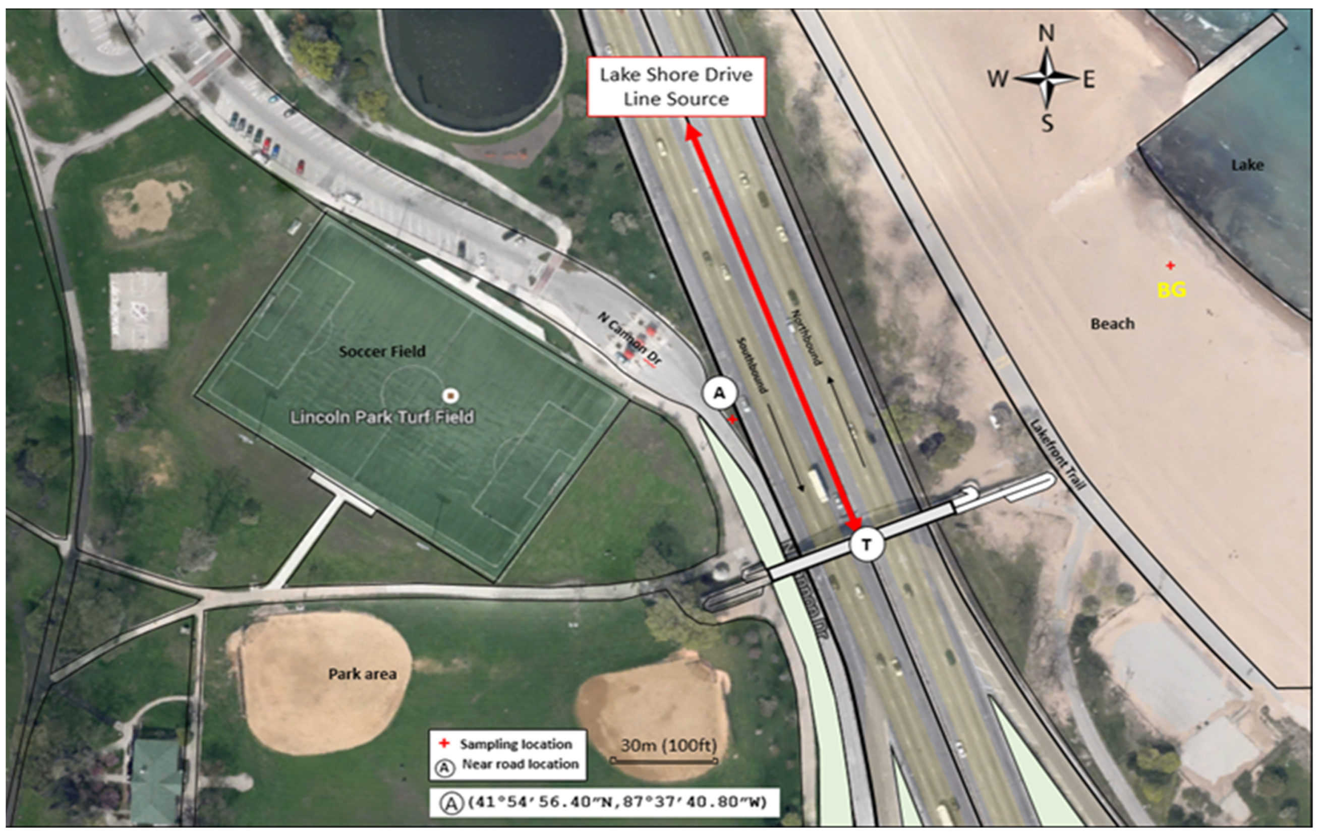
The sampling program near LSD (two hundred five-minute samples) was conducted at North Avenue (41°54′56.40″ N, 87°37′40.80″ W) in Chicago, IL, USA. Figure 1 presents the LSD sampling site. The LSD site is near Lake Michigan and is surrounded by level terrain and short grass with no elevations. The freeway is at grade with 8 lanes without highway barriers. LSD is restricted to LDVs only. LDVs are transport passenger and cargo vehicles, including cars, SUVs, and pickup trucks. EPA classifies a vehicle as light-duty when the gross vehicle weight is under 8500 lbs. The average traffic volume was near 150,000 (veh day−1) [39].
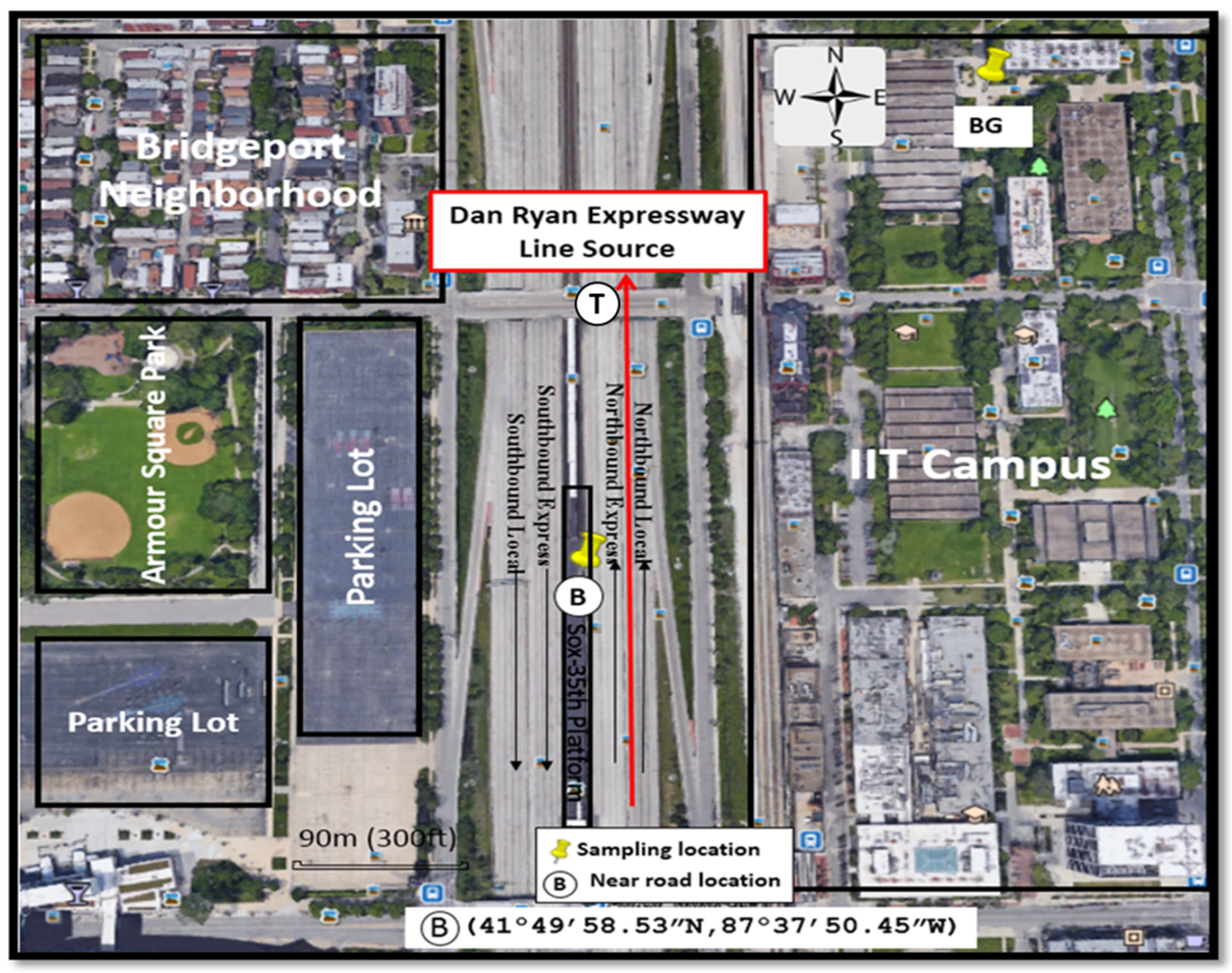
The DRE sampling program (four hundred five-minute samples) was near an urban highway next to the Illinois Institute of Technology campus (41°49′58.53″ N, 87°37′50.45″ W) in Chicago, IL, USA. Figure 2 presents a map of the sampling site including near road and background sampling locations. DRE is situated 6 m below the adjacent terrain, flanked by a parking lot on one side and low-rise structures on the other. The freeway has 14 lanes (8 express lanes, 6 local lanes), separated into north and southbound roadways by a 10 m wide subway platform. The express lanes are restricted to LDVs, and the local lanes are open to both LDVs and HDVs. HDV stands for vehicles with over 8500 lbs. of gross vehicle weight based on EPA emissions and fuel economy certification, which include school and public transit buses, freight, and other fleet vehicles with a weight between 25,000 and 35,000 lbs. Information from the Illinois Department of Transportation [39] provided annual average daily traffic flow rates of 300,000 (veh day−1) with 8.4% HDVs.
Sampling dates were chosen based on stable weather conditions to minimize background uncertainties and mitigate the impact of unforeseen weather events on near-road turbulence measurements. This entailed selecting days with consistent easterly winds and a stable atmospheric stability class in the background.
The sampling procedure was meticulously executed utilizing handheld instruments capable of rapid response. These devices were engaged at five-minute intervals, spanning a duration of 2 to 3 h, a timeframe that was contingent upon prevailing traffic and meteorological conditions. Throughout the sampling program, the prevailing ambient horizontal wind directions recorded ranged from northeast to southeast at both LSD and DRE locations. LSD measurements were made at the edge of the roadway (site A) and 100 m upwind for the background. For DRE, measurements were made in the middle of the roadway using the CTA platform (site B) and 200 m upwind from the road edge for the background. Wind speed alongside traffic metrics, encompassing flow and speed, were concurrently measured in sync with TKE computations at five-minute intervals. TKE was determined every five minutes using Equation (1) with three-dimensional wind variance based on three hundred data points collected from three-directional (parallel, perpendicular, vertical) wind velocities. These directional wind speeds were recorded every second using a 3-D sonic anemometer (Gill Instruments Limited, Lymington, Hampshire, UK)with a 1 Hz frequency. The average horizontal wind speed over a five-minute interval can be deduced from the parallel and perpendicular wind speeds recorded using the 3-D sonic anemometer. These data were corroborated using the results measured independently using a Kestrel 4500 handheld wind meter (Nielsen-Kellerman Company, Boothwyn, PA, USA) (see also Supplementary Materials). The real-time horizontal wind speed displayed on the Kestrel 4500 facilitated a provisional estimation of the turbulence level during each five-minute measurement interval, aiding in the interpretation of any TKE biases that may arise due to unforeseen gusty conditions. The traffic information was recorded on an overpass that allowed all lanes of traffic to be recorded. A video recorder (Sony HDR-CX330, Sony Corporation, Konan, Minato, Tokyo) was deployed to document the traffic conditions, encompassing traffic flow and speed, in each five-minute interval. The recorded traffic conditions were categorized into two distinct phases: congestion (where the average vehicle speed was less than 60 km/h) and free flow (where the average vehicle speed was 60 km/h or greater) for the LSD. However, in the case of the DRE, the delineation between congestion and free flow was modified to range from 50 to 70 km/h, owing to the significant influence of HDVs in that area. The two selected sampling highways encompass a comprehensive range of traffic conditions; thus, the results obtained, which are synchronized with traffic conditions, possess universal applicability.
2.2. Traffic-Induced TKE
Near-roadway traffic-induced and background TKE were determined using the following equation [29]:
where TKEt is total TKE near the road (m2 s−2) and TKEb is background TKE (m2 s−2). TKEtr refers to traffic-induced TKE (m2 s−2) at the near-road location, which can be substituted with LDV-generated TKE (TKELDV) due to the LDV-only traffic fleet on LSD. On DRE, TKEtr also includes HDV-generated TKE (TKEHDV) since the traffic fleet is a mixture of LDVs and HDVs. The mixed traffic induced TKE on DRE is calculated by substituting TKEtr with TKELDV plus TKEHDV as shown in Equation (3):
In Equation (3), TKELDV was determined using Equation (4) for LSD. The reason for applying the TKE from LSD LDVs is because of the similar LDV model, where traffic condition includes a range of flow rates and speed.
2.3. Near-Road Characterization of TKE and Three-Dimensional Wind STD
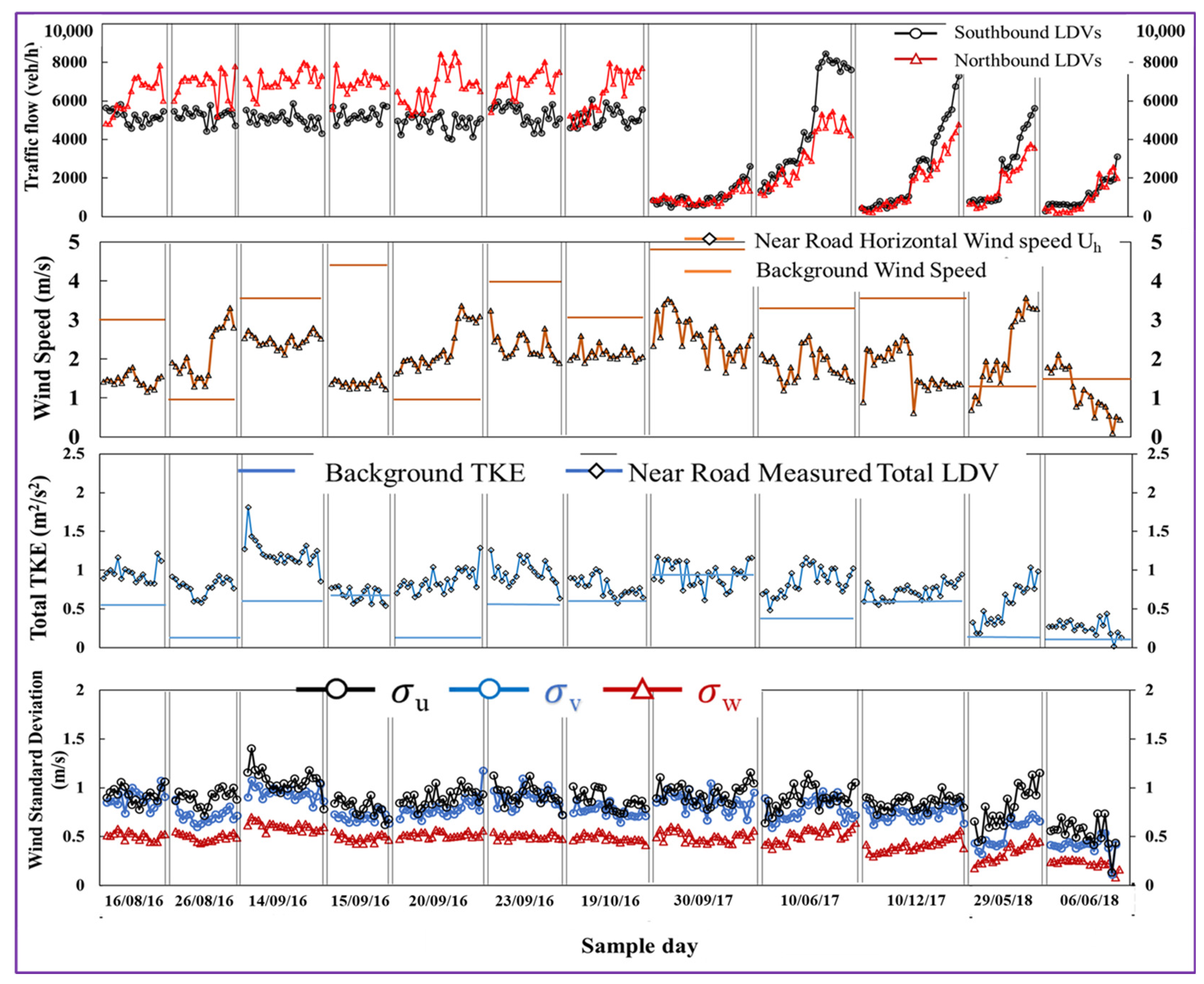
Figure 3 provides information on five-minute measurements for LSD. To evaluate the TKE results in steady- and unsteady-state traffic conditions, sampling near LSD was divided into a daytime sample and a nighttime sample. Day sampling was conducted between 16 August 2016 and 19 October 2016 between 2 pm and 6 pm, where the traffic was in free flow or congestion with LDVs flow rates up to 13,000 (veh h−1). Night sampling was conducted between 30 September 2017 and 6 June 2018 between 2 am and 6 am, where the traffic was in free flow but the number of LDVs was 500 (veh h−1), which is much smaller than in the daytime. Horizontal wind speed ranged from 0.5 to 3.5 m/s and was from the east. The near-road TKEt averaged 0.9 (m2 s−2) (0.3 STD). The average background TKE (TKEb) was 0.3 (m2 s−2). Wind STD in the horizontal plane was near 1 (m/s), and parallel averaged wind STD σu was 10% higher than perpendicular wind STD.
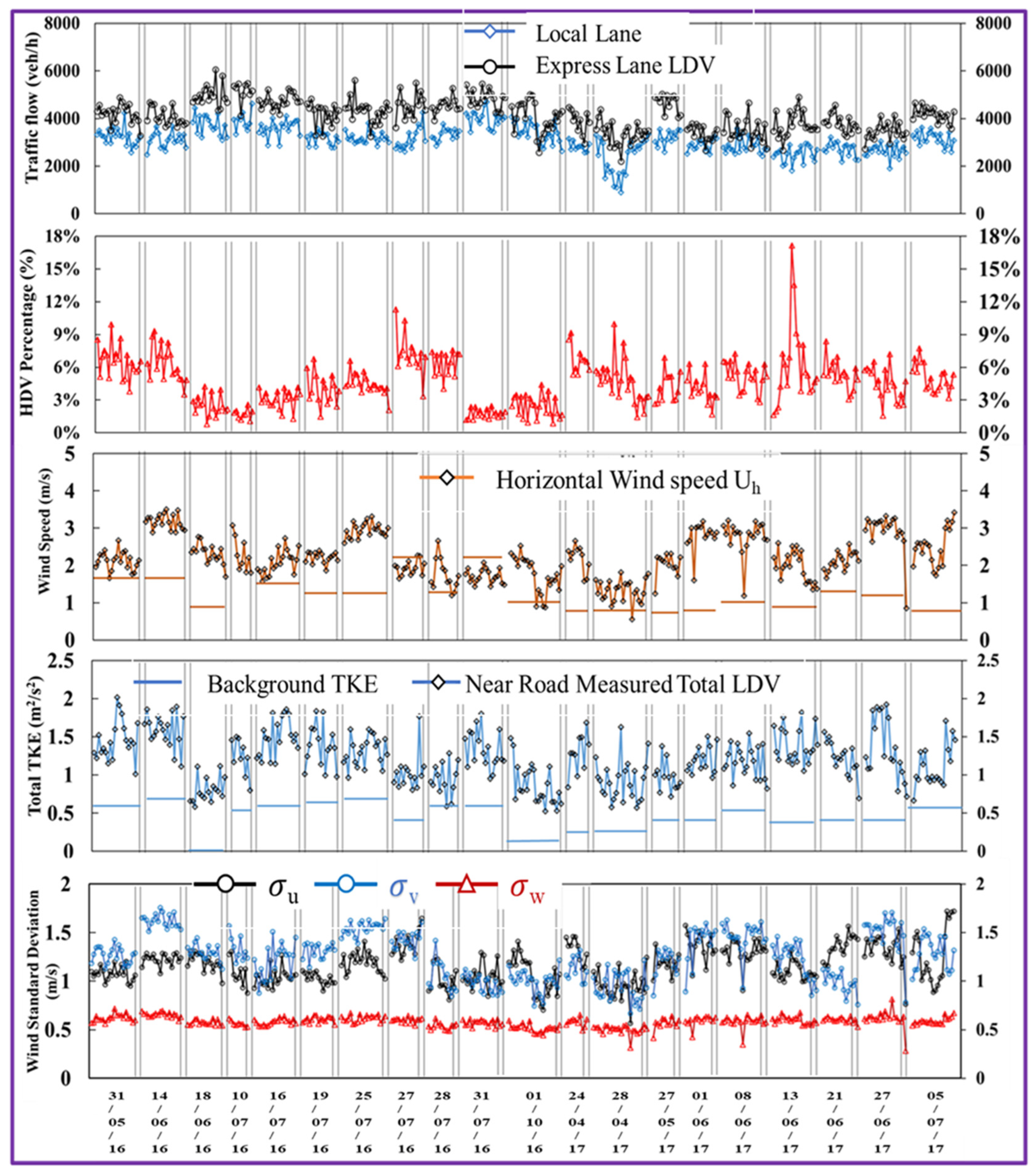
Figure 4 provides the measurements for DRE. The average traffic flow rate was 8000 (veh h−1), which was smaller than that of LSD. The percentage of HDVs in the traffic fleet averaged 8.4%, with variation from 1 to 18%. Wind speed ranged from 1 to 3.5 m/s and was from the east during sampling days. The background DRE wind speed was smaller than that of LSD. The DRE TKEt averaged 1.2 (m2 s−2) (0.4 STD). TKEb averaged 0.4 (m2 s−2). Wind STD in the horizontal plane was near 1.3 (m/s), in contrast to LSD.
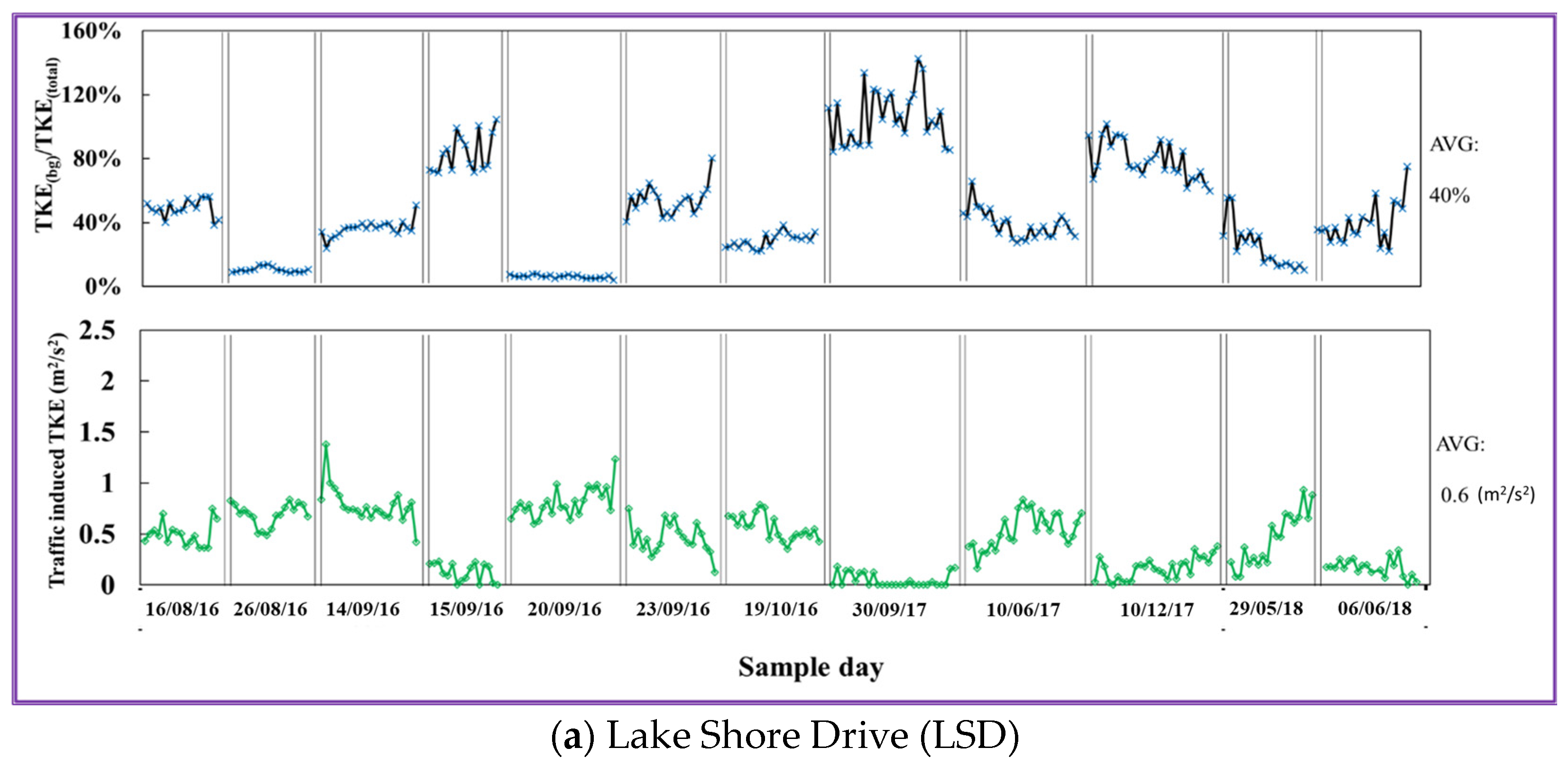
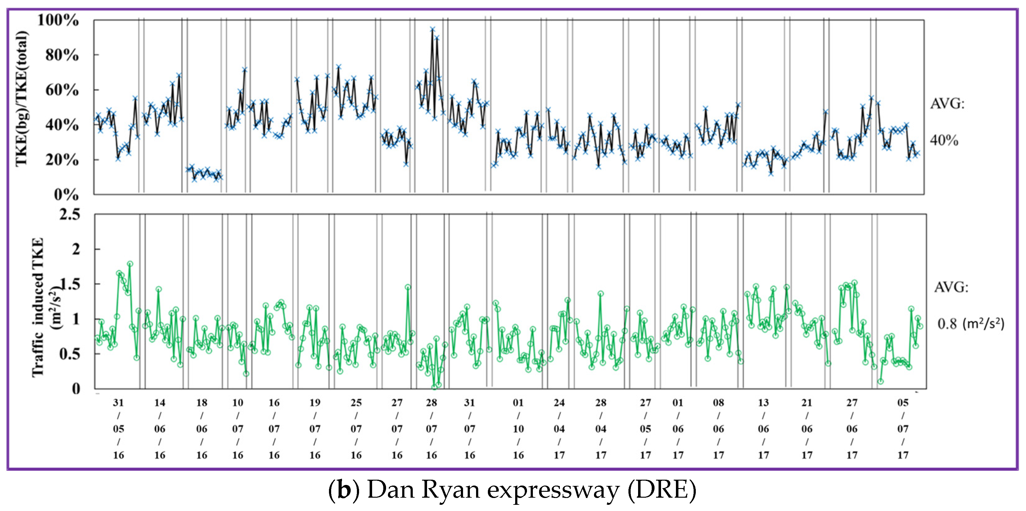
Figure 5 presents the relationship between the TKEb, TKEtr, and TKEt ratio between TKEb and TKEt and the value of TKEtr. The results indicate that the average ratio of TKEb to TKEt was 40%, and the TKEtr was near 0.8 (m2 s−2) (0.3 STD) on LSD. Near-road TKEtr on DRE was 30% higher than on LSD. The ratio of TKEb and TKEt was 40%. TKELDV averaged 0.6 (m2 s−2) (0.2 STD). The results also indicate the standard error of TKEt and TKEtr were higher on DRE, and the influence of different traffic types, flow rates, and speed between the two sampling sites on TKEt and TKEtr were evaluated.
3. Results
3.1. TKE and Wind STD
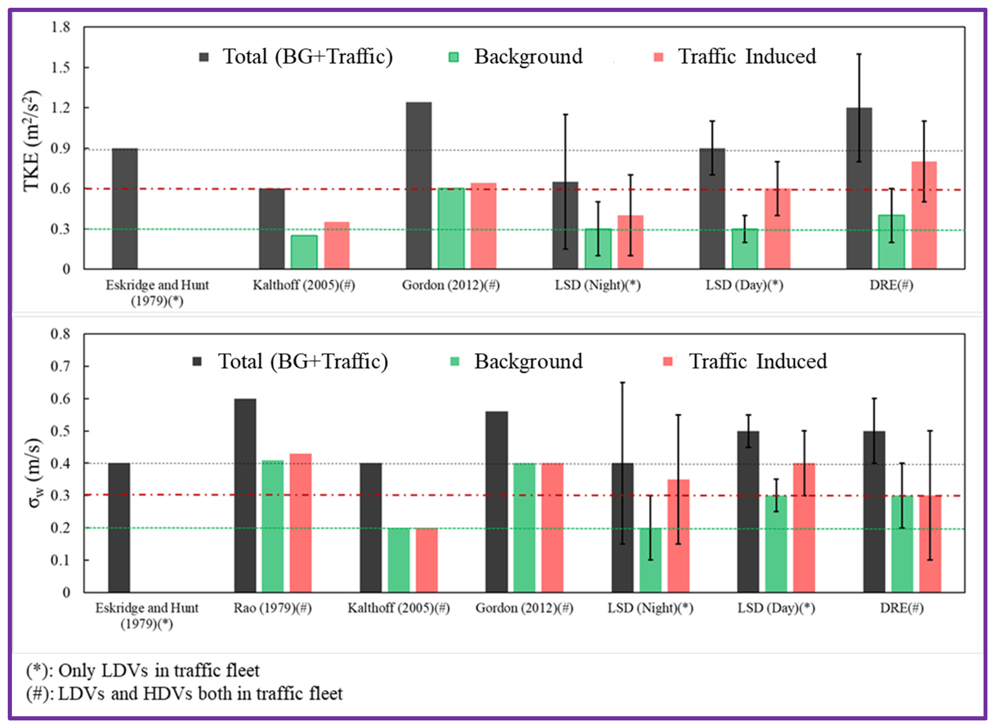
TKE and vertical wind STD from previous near-road studies are summarized in Figure 6 along with the results from this study for LSD and DRE. In Figure 6, previous near-road measurements indicate that near-road TKEt is between 0.6 and 1.2 (m2 s−2), TKEb is between 0.2 and 0.6 (m2 s−2), and TKEtr is between 0.35 and 0.64 (m2 s−2). From the LSD and DRE measurements, the average TKEt is between 0.5 and 1.2 (m2 s−2), TKEb is near 0.35 (m2 s−2), and the average TKEtr is between 0.4 and 0.8 (m2 s−2). The results of average TKEtr from LSD and DRE are comparable to the previous near-road studies. However, in previous studies conducted near roads, variations in TKEtr were primarily attributed to background changes, given the marginal influence of different traffic types, particularly the low percentage of HDVs in the traffic fleet. Moreover, the TKE generated by HDVs over extended periods is too negligible to measure due to the rapid dissipation of energy. In this study, the influence of TKEHDV was quantified, with measurements particularly focused on short-duration intervals.
Figure 6 also shows the vertical wind STD σw from all the studies are near 0.3 (m/s), which indicates the measured traffic pattern is comparable to the previous since σw is dominated by traffic at near-road locations. Combined with previous studies, the TKEtr from 0.2 (m2/s2) to 1.0 (m2/s2) includes the influence of the steady-state traffic fleet flow (TKEtr is around 0.6 m2/s2) and shows the unsteady-state traffic fleet flow influence (TKEtr is around 0.3 m2/s2). The influence of TKEHDV is shown as high TKEtr on DRE (TKEtr is up to 1.0 m2/s2).
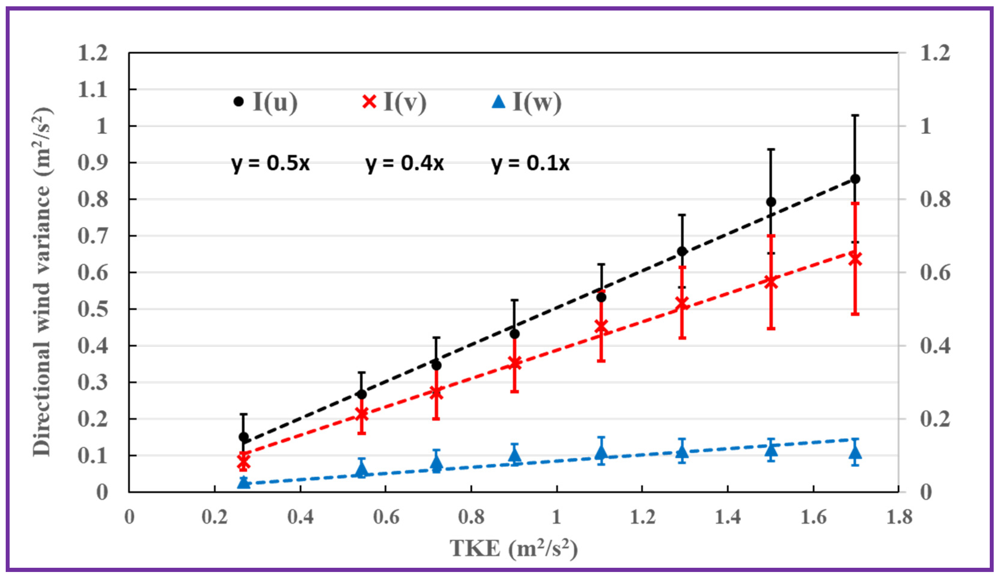
The changes in TKE as a function of directional wind STD are shown in Figure 7 to identify the relationship between directional wind variance and TKE. In this study, the observed wind variance, calculated with standard deviation (STD) in the horizontal plane (both parallel and perpendicular), exhibited an increase correlating with TKE. The data suggest that σu2 and σv2 contributed to 50% and 40% of the TKE, respectively, while σw2 accounted for a mere 10% contribution to the TKE. Furthermore, the analysis indicates a consistent ratio between wind variance and TKE, which can be utilized to assess directional wind variance based on measured TKE under varying traffic conditions.
3.2. TKEtr as a Function of Traffic Conditions
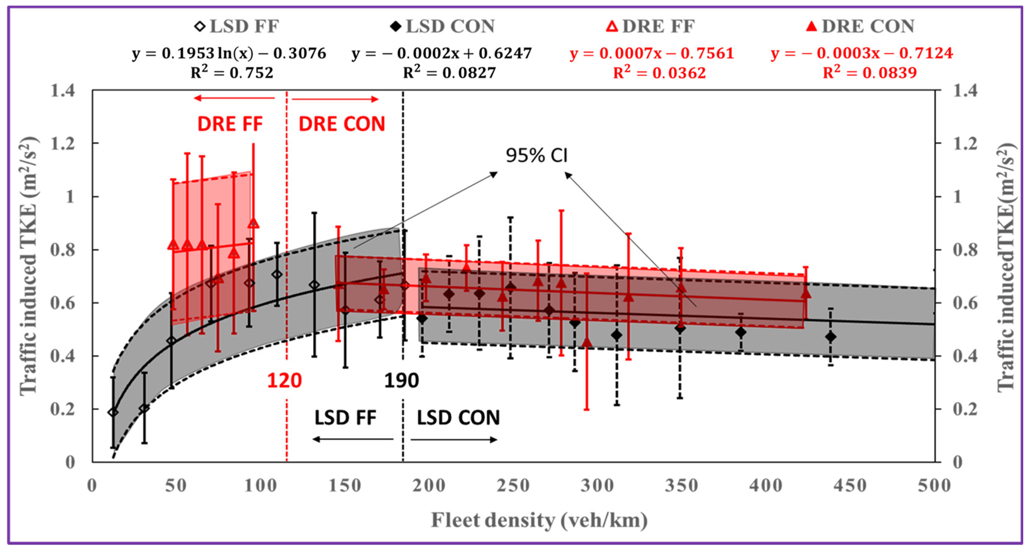
Previous research has established that traffic conditions—encompassing both traffic fleet flow rates and speeds—significantly influence TKEtr generation. To facilitate a comprehensive assessment of TKEtr within the full scope of traffic patterns, we introduce a parameter termed “traffic density”. This parameter, delineated in Equation (5), represents traffic conditions by incorporating the effects of both traffic speed and flow rate.
where k is the traffic density (veh km−1), N is the traffic flow rate (veh h−1), and V is the traffic velocity (km h−1). TKEtr is calculated every five minutes, and the values are highly variated, especially on DRE because of the HDV influence, so the five-minute ensemble mean of TKEtr and k are calculated to organize the variation. The change in the TKEtr ensemble mean as a function of traffic density is shown in Figure 8.
The 95% confidence intervals are presented in Figure 8 to compare the variations in TKEtr in DRE and LSD, where “k” ranges from 0 to 350 (veh km−1) and discerns the range of traffic conditions from free flow to congestion. The extensive variations in traffic density encapsulate the entire spectrum of service levels within the transportation sector, consequently giving rise to a broad range of TKEtr values, as mentioned in the Introduction. Given the universal nature of traffic types, the TKEtr results from LSD and DRE are comparable. A density value approaching 0 (veh km−1) signifies reduced traffic flow rates coupled with higher speeds, whereas a value approaching 350 (veh km−1) indicates a reversal in traffic conditions, characterized by diminished speeds and increased flow rates. The thresholds distinguishing traffic free flow and congestion are predicated on the measured traffic speeds on both LSD and DRE, respectively. Under the threshold traffic speed (V), the threshold k is 120 (veh km−1) for DRE and 190 (veh km−1) for LSD.
Results from LSD show that the LDV-induced TKEtr (TKELDV) increases from 0.07 to 0.6 (m2 s−2) when LDV density increases from 10 to 100 (veh km−1). This means the TKEtr increases when the traffic amounts increase under the unsteady state. After LDV density passes 100 (veh km−1), the TKEtr becomes relative constant at 0.6 m2/s2, which means the LDV reaches steady-state flow and TKEtr stays similar even in very congested traffic (near 350 veh km−1). Based on the traffic measurements from DRE, the presence of HDVs in the traffic fleet results in a more confined range of free flow density (k) compared with LSD, although the k range indicative of congestion remains consistent across both locations. The result from DRE shows that TKEtr is 0.8 (m2 s−2) (0.3 STD) for DRE free flow and 0.7 (m2 s−2) (0.2 STD) for congestion.
Given the low correlation coefficient (R2 < 0.1 for both congestion and free flow) observed in the function relating TKEtr to k on DRE, it can be concluded that TKEtr shares no correlation with k. This condition can be attributed to the predominant presence of LDVs in the traffic fleet maintaining a steady-state flow, resulting in an unaltered TKEtr that is not influenced by changing traffic conditions. The correlation analysis further reveals an absence of correlation between TKEtr and k on LSD and DRE during periods of decelerating traffic that transitions into a steady state. Conversely, the correlation coefficient for LSD during free-flow conditions markedly exceeds that observed in the other three traffic scenarios (LSD congestion, DRE free flow, and congestion). This discrepancy can be attributed to a positive correlation between TKEtr and k when LDVs operate under unsteady flow conditions. The correlation analysis concludes that in traffic flows dominated by LDVs, a distinct pattern shows that during periods of unsteady flow, an increase in k is accompanied by an increase in TKEtr, exhibiting a high correlation. Conversely, in situations where LDVs maintain a steady-state flow, TKEtr appears to remain unaffected, demonstrating no discernible correlation with the traffic conditions.
Figure 8 also shows that even if the LDVs dominated steady-state traffic flow, TKEtr is still larger in DRE under free-flow conditions, which is due to the impact of HDVs. The average TKEtr on DRE increases by 30% compared with LSD, even if the HDV percentage is only near 8.3% on DRE.
3.3. The Influence of HDV on Near-Road TKEtr
Six five-minute samples from LSD and DRE for TKE are listed in Table 1 with the simultaneously measured traffic conditions in Table 2 to evaluate the influence of HDVs. The traffic fleet flow rate is from 6500 to 7500 (veh h−1), with similar LDV flow rates at near 6800 (veh h−1) and increasing HDV flow. The vehicle speed is between 85 and 120 (km h−1) as a free-flow condition. Based on the data presented in Figure 8, it can be deduced that the traffic fleet maintains a steady-state flow on both LSD and DRE. The measured TKEtr increases from 0.54 to 1.09 (m2 s−2) with the HDV flow rates increasing from 0 to 660 (veh h−1) and similar LDV flow rates. The data corresponding to Figure 8 underscores that the influence of HDVs is substantial enough to disrupt the steady-state flow typically sustained by LDV traffic patterns.
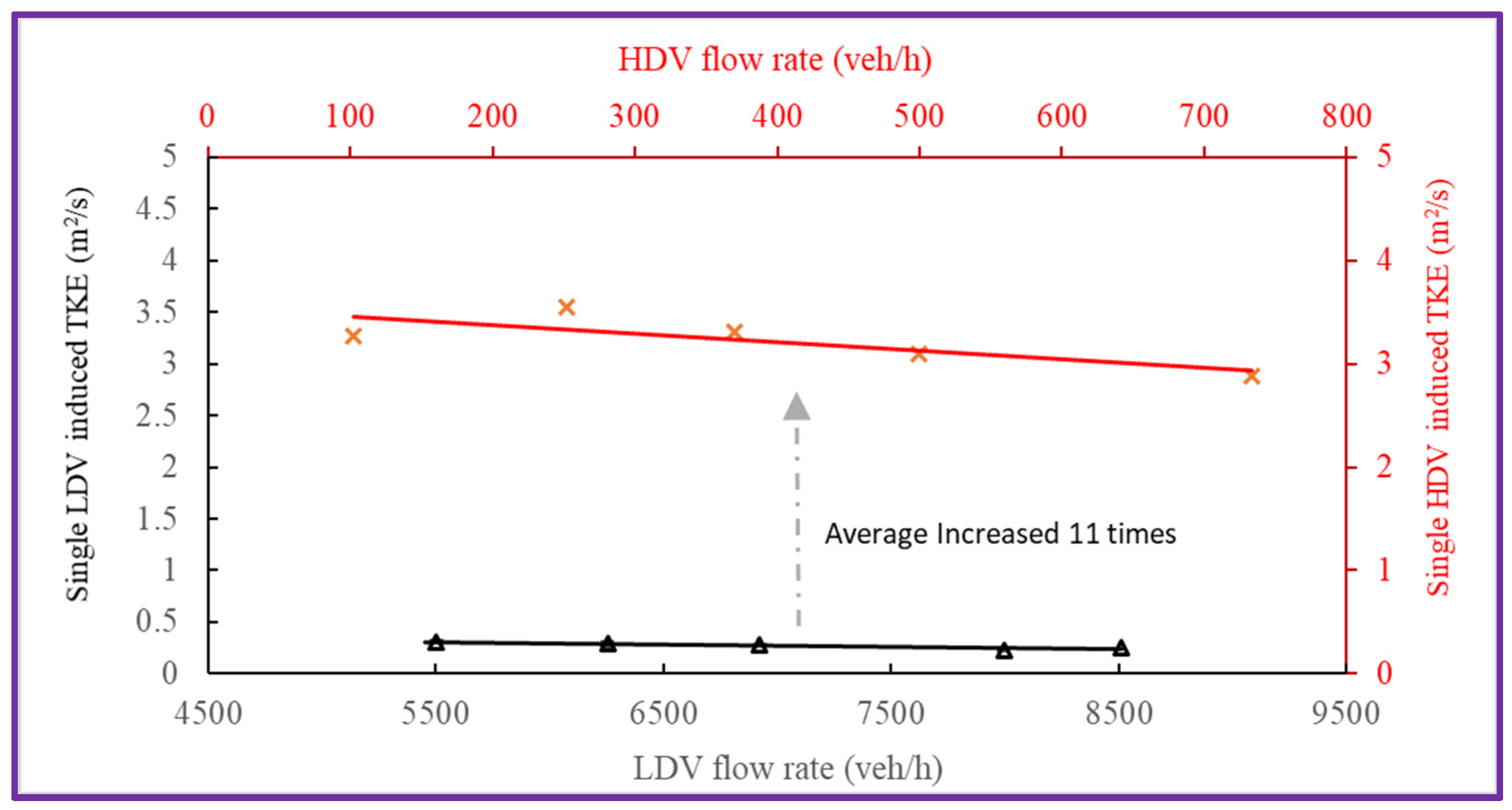
Table 1 shows the results for normalized TKEtr, which represents the single-vehicle TKEtr derived from subdivided measurements (TKELDV and TKEHDV) and respective LDV or HDV flow rates. This normalized metric indicates an individual vehicle’s impact on near-road turbulence measurements, with background influences effectively negated by the application of Equation (3). Figure 9 illustrates the ratio of normalized TKEHDV to TKELDV, reaching a value of up to 11. This denotes that the measured TKEHDV can be up to 10 times greater than the measured TKELDV on a single-vehicle basis, thereby quantifying the substantial influence of HDVs on near-road TKE measurements.
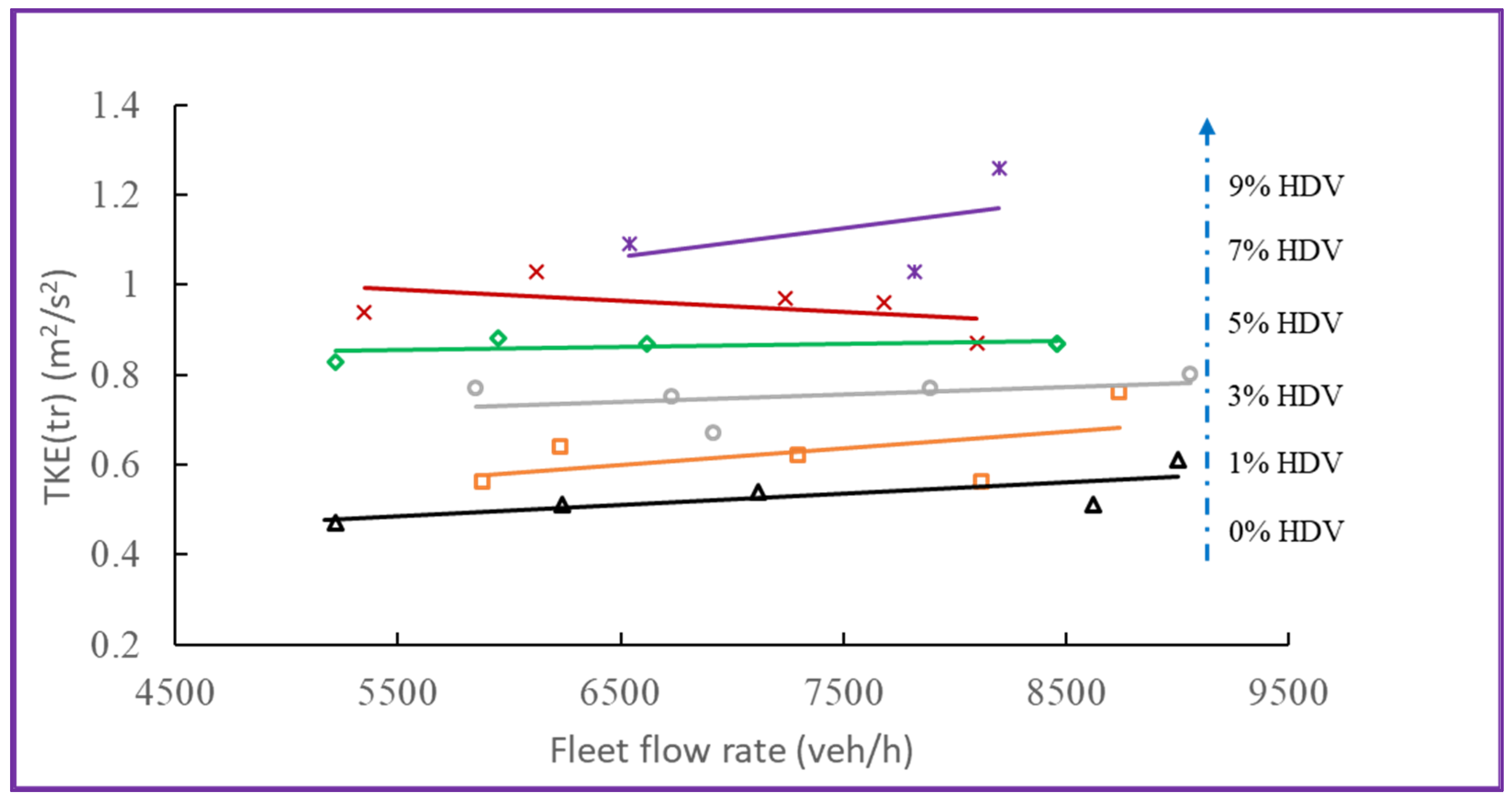
Figure 10 substantiates the impact of HDVs on TKEtr, delineating the fluctuations as a function of fleet flow rate from 5000 to 9000 veh h−1. The analysis further illustrates a subdivision of TKEtr by the increasing HDV percentage; it demonstrates that TKEtr augments from 0.4 to 1.2 (m2 s−2) as the HDV percentage increases from 0 to 9%. This trend persists even when LDV counts increase from 5000 to 9000 (veh h−1) at a consistent HDV percentage, thereby corroborating the stability of TKEtr under LDV steady-state flow.
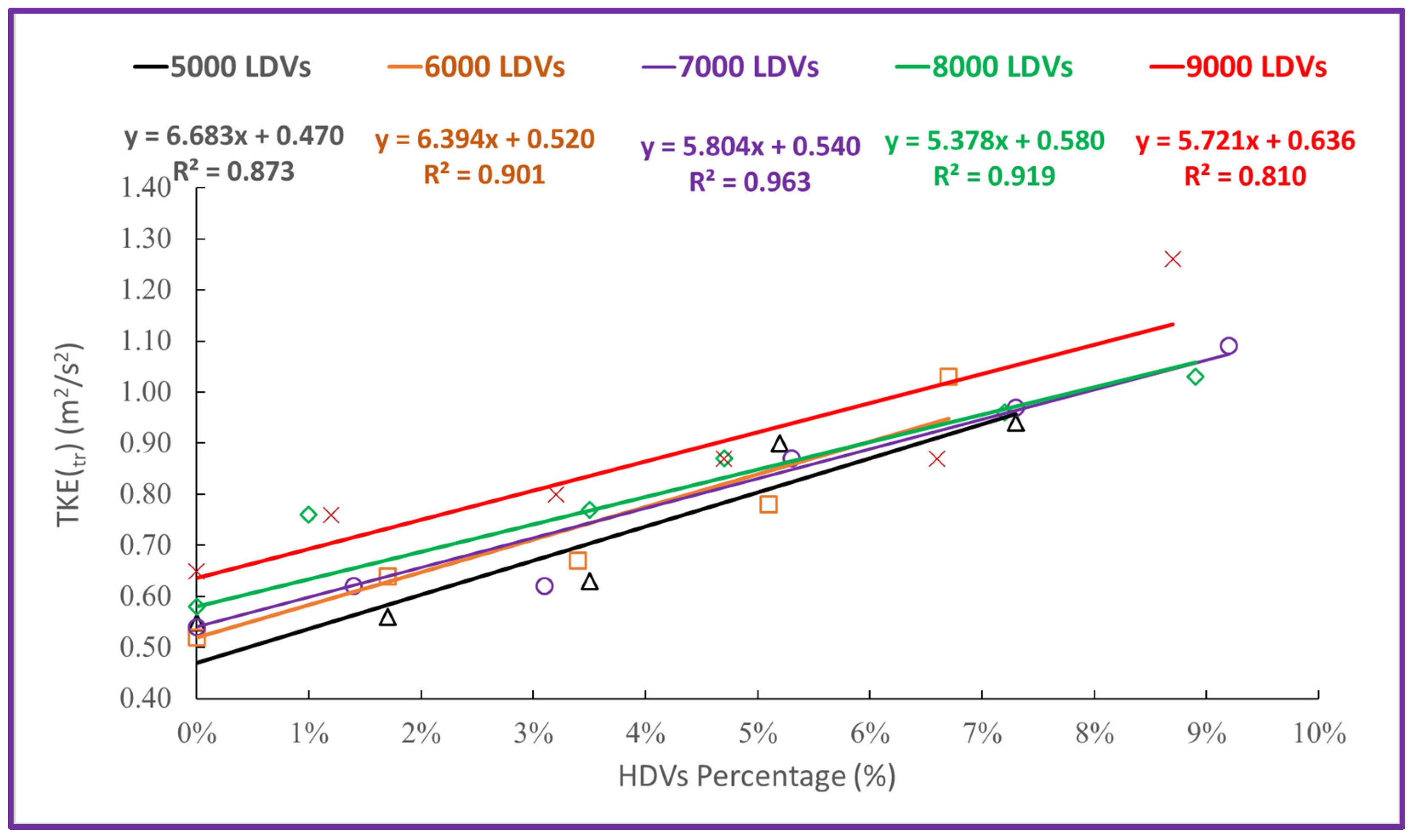
Figure 11 shows the changes in TKEtr as a function of HDV percentage by subdividing the results from 5000 veh h−1 to 9000 veh h−1 of LDV flows. Linear regression is utilized to discern the linear relationship between TKEtr and the percentage of HDVs within specific LDV flows. This analysis reveals a moderate to strong positive correlation, as evidenced by a correlation coefficient ranging from 0.81 to 0.96. The results, as illustrated in Figure 10, demonstrate that the influence of LDV flow on TKEtr is minimal when steady-state flow is established, with the percentage of HDVs predominantly and positively relating to the trends in TKEtr variations.
4. Conclusions
To bridge the existing void in scholarly literature and furnish a comprehensive assessment of turbulent kinetic energy (TKEtr) within the full spectrum of traffic conditions, an exhaustive exploration of various traffic patterns is imperative. In this study, we conducted the calculation of TKEtr over five-minute intervals, synchronously analyzing traffic conditions using simultaneous traffic measurements. Furthermore, we delineated the relationship between wind variance and TKE, which confirmed a stable relationship, evaluated the impact of heavy-duty vehicles (HDVs) within the traffic fleet based on short-duration sampling near roads and assessed TKEtr in relation to shifts in density during both free-flow and congestion phases.
The results illustrate that TKEtr escalates in tandem with traffic density (k) yet stabilizes when the traffic fleet achieves a sufficient traffic density (k) to maintain a steady-state flow, predominantly attributed to the prevalence of LDVs. The correlation analyses signify a lack of correlation between k and TKEtr during periods of steady-state flow characterized by LDV dominance within the traffic fleet. Conversely, a positive correlation is observed when LDVs are experiencing unsteady-state flow conditions.
The analysis pertaining to TKEHDV clearly indicates that the TKEHDV can be up to tenfold higher compared with TKELDV on an individual vehicle basis, thereby underscoring the pronounced influence of HDVs on proximate roadway TKE measurements. Furthermore, the TKEtr trend maintains its course even as the LDV volume escalates from 5000 to 9000 (veh h−1), maintaining a uniform HDV percentage and thus affirming the stability of TKEtr during periods of LDV steady-state flow. The correlation analyses demonstrate that the LDV flow exerts a negligible impact on TKEtr during the establishment of a steady-state flow, with the HDV proportion predominantly relating to the variations in TKEtr, exhibiting a positive correlation.
In this study, both steady and unsteady states of LDV flows were clearly delineated. However, it was observed that the presence of HDVs could escalate TKEtr levels even during phases of LDV steady flow. Given the observed stability in LDV flows, we hypothesize the existence of a corresponding steady-state flow for HDVs; a state characterized by a sufficient volume of HDVs to maintain a consistent TKEHDV irrespective of fluctuating traffic conditions. Intriguingly, this hypothesized steady state for HDVs remained elusive throughout this study, even on the DRE, where HDVs constituted up to 14% of traffic. Identifying the precise HDV percentage that facilitates a steady-state flow within the traffic fleet necessitates further exploration, potentially utilizing aerodynamic modeling tools such as computational fluid dynamics (CFD) in subsequent analyses.
Furthermore, this near-road measurement initiative is poised to refine the existing near-road air dispersion model. This improved version aims to offer a more precise estimation of near-road traffic emissions by integrating facets of real-world traffic conditions, emission dispersion, and traffic-induced turbulence into a unified framework, leveraging data obtained using five-minute near-road sampling.
Supplementary Materials
The following supporting information can be downloaded at: https://www.mdpi.com/article/10.3390/atmos14101485/s1.
Author Contributions
Conceptualization, Z.H. and K.E.N.; methodology, Z.H. and K.E.N.; software, Z.H.; validation, Z.H. and K.E.N.; formal analysis, Z.H.; investigation, Z.H.; resources, Z.H.; data curation, Z.H.; writing—original draft preparation, Z.H.; writing—review and editing, Z.H.; visualization, Z.H.; supervision, K.E.N.; project administration, K.E.N. All authors have read and agreed to the published version of the manuscript.
Funding
This research received no external funding.
Institutional Review Board Statement
Not Applicable.
Informed Consent Statement
Not Applicable.
Data Availability Statement
Data to this article can be found in the Supplementary Materials. Additional information are available on request from the corresponding author.
Conflicts of Interest
The authors declare no conflict of interest.
References
- Baker, C. Outline of a Novel Method for the Prediction of Atmospheric Pollution Dispersal from Road Vehicles. J. Wind Eng. Ind. Aerodyn. 1996, 65, 395–404. [Google Scholar] [CrossRef]
- Bäumer, D.; Vogel, B.; Fiedler, F. A New Parameterisation of Motorway-Induced Turbulence and Its Application in a Numerical Model. Atmos. Environ. 2005, 39, 5750–5759. [Google Scholar] [CrossRef]
- Eskridge, R.E.; Rao, S.T. Measurement and Prediction of Traffic-Induced Turbulence and Velocity Fields Near Roadways. J. Appl. Meteorol. 1983, 22, 1431–1443. [Google Scholar] [CrossRef]
- Rao, K.; Gunter, R.; White, J.; Hosker, R. Turbulence and Dispersion Modeling Near Highways. Atmos. Environ. 2002, 36, 4337–4346. [Google Scholar] [CrossRef]
- Venkatram, A.; Isakov, V.; Thoma, E.; Baldauf, R. Analysis of Air Quality Data near Roadways Using a Dispersion Model. Atmos. Environ. 2007, 41, 9481–9497. [Google Scholar] [CrossRef]
- Morawska, L.; Jamriska, M.; Thomas, S.; Ferreira, L.; Mengersen, K.; Wraith, D.; McGregor, F. Quantification of Particle Number Emission Factors for Motor Vehicles from On-Road Measurements. Environ. Sci. Technol. 2005, 39, 9130–9139. [Google Scholar] [CrossRef]
- Jamriska, M.; Morawska, L. A model for determination of motor vehicle emission factors from on-road measurements with a focus on submicrometer particles. Sci. Total Environ. 2000, 264, 241–255. [Google Scholar] [CrossRef]
- Eskridge, R.E.; Petersen, W.B.; Rao, S.T. Turbulent Diffusion Behind Vehicles: Effect of Traffic Speed on Pollutant Concentrations. J. Air Waste Manag. Assoc. 1991, 41, 312–317. [Google Scholar] [CrossRef]
- Eskridge, R.E.; Hunt, J.C.R. Highway Modeling. Part I: Prediction of Velocity and Turbulence Fields in the Wake of Vehicles. J. Appl. Meteorol. 1979, 18, 387–400. [Google Scholar] [CrossRef]
- He, M.; Dhaniyala, S. A Dispersion Model for Traffic Produced Turbulence in a Two-Way Traffic Scenario. Environ. Fluid Mech. 2011, 11, 627–640. [Google Scholar] [CrossRef]
- Watkins, S.; Saunders, J.W.; Hoffmann, P.H. Turbulence Experienced by Moving Vehicles. Part I. Introduction and Turbulence Intensity. J. Wind Eng. Ind. Aerodyn. 1995, 57, 1–17. [Google Scholar] [CrossRef]
- Wu, M.; Li, Y.; Chen, X.; Hu, P. Wind Spectrum and Correlation Characteristics Relative to Vehicles Moving through cross Wind Field. J. Wind Eng. Ind. Aerodyn. 2014, 133, 92–100. [Google Scholar] [CrossRef]
- Gidhagen, L.; Johansson, C.; Omstedt, G.; Langner, J.; Olivares, G. Model Simulations of NOx and Ultrafine Particles Close to a Swedish Highway. Environ. Sci. Technol. 2004, 38, 6730–6740. [Google Scholar] [CrossRef] [PubMed]
- Kim, Y.; Huang, L.; Gong, S.; Jia, C.Q. A New Approach to Quantifying Vehicle Induced Turbulence for Complex Traffic Scenarios. Chin. J. Chem. Eng. 2016, 24, 71–78. [Google Scholar] [CrossRef]
- Sahlodin, A.M.; Sotudeh-Gharebagh, R.; Zhu, Y. Modeling of Dispersion near Roadways Based on the Vehi-cle-Induced Turbulence Concept. Atmos. Environ. 2007, 41, 92–102. [Google Scholar] [CrossRef]
- Wang, Y.J.; Nguyen, M.T.; Steffens, J.T.; Tong, Z.; Wang, Y.; Hopke, P.K.; Zhang, K.M. Modeling Multi-Scale Aerosol Dynamics and Micro-Environmental Air Quality near a Large Highway Intersection Using the CTAG Model. Sci. Total Environ. 2013, 443, 375–386. [Google Scholar] [CrossRef]
- Wang, Y.J.; Zhang, K.M. Coupled Turbulence and Aerosol Dynamics Modeling of Vehicle Exhaust Plumes Using the CTAG model. Atmos. Environ. 2012, 59, 284–293. [Google Scholar] [CrossRef]
- Carpentieri, M.; Kumar, P.; Robins, A. Wind Tunnel Measurements for Dispersion Modelling of Vehicle Wakes. Atmos. Environ. 2012, 62, 9–25. [Google Scholar] [CrossRef]
- Cheli, F.; Corradi, R.; Sabbioni, E.; Tomasini, G. Wind Tunnel Tests on Heavy Road Vehicles: Cross Wind Induced Loads—Part 1. J. Wind Eng. Ind. Aerodyn. 2011, 99, 1000–1010. [Google Scholar] [CrossRef]
- Cheli, F.; Ripamonti, F.; Sabbioni, E.; Tomasini, G. Wind Tunnel Tests on Heavy Road Vehicles: Cross Wind Induced Loads—Part 2. J. Wind Eng. Ind. Aerodyn. 2011, 99, 1011–1024. [Google Scholar] [CrossRef]
- Eskridge, R.E.; Thompson, R.S. Experimental and Theoretical Study of the Wake of a Block-Shaped Vehicle in A Shear-Free Boundary Flow. Atmos. Environ. 1982, 16, 2821–2836. [Google Scholar] [CrossRef]
- Heist, D.K.; Perry, S.G.; Brixey, L.A. A Wind Tunnel Study of the Effect of Roadway Configurations on the Dispersion of Traffic-Related Pollution. Atmos. Environ. 2009, 43, 5101–5111. [Google Scholar] [CrossRef]
- Kastner-Klein, P.; Fedorovich, E.; Rotach, M. A Wind Tunnel Study of Organised and Turbulent Air Motions in Urban Street Canyons. J. Wind Eng. Ind. Aerodyn. 2001, 89, 849–861. [Google Scholar] [CrossRef]
- Lo, K.H.; Kontis, K. Flow around an Articulated Lorry Model. Exp. Therm. Fluid Sci. 2017, 406, 58–74. [Google Scholar] [CrossRef]
- McAuliffe, B.R.; Belluz, L.; Belzile, M. Measurement of the On-Road Turbulence Environment Experienced by Heavy Duty Vehicles. SAE Int. J. Commer. Veh. 2014, 7, 685–702. [Google Scholar] [CrossRef]
- McArthur, D.; Burton, D.; Thompson, M.; Sheridan, J. On the near Wake of a Simplified Heavy Vehicle. J. Fluids Struct. 2016, 66, 293–314. [Google Scholar] [CrossRef]
- Alonso-Estébanez, A.; Pascual-Muñoz, P.; Yagüe, C.; Laina, R.; Castro-Fresno, D. Field Experimental Study of Traffic-Induced Turbulence on Highways. Atmos. Environ. 2012, 61, 189–196. [Google Scholar] [CrossRef]
- Belušić, D.; Lenschow, D.H.; Tapper, N.J. Performance of a Mobile Car Platform for Mean Wind and Turbulence Measurements. Atmos. Meas. Tech. 2014, 7, 1825–1837. [Google Scholar] [CrossRef]
- Gordon, M.; Staebler, R.M.; Liggio, J.; Makar, P.; Li, S.M.; Wentzell, J.; Lee, P.; Brook, J.R. Measurements of En-hanced Turbulent Mixing near Highways. J. Appl. Meteorol. Climatol. 2012, 51, 1618–1632. [Google Scholar] [CrossRef]
- Rao, S.T.; Sedefian, L.; Czapski, U.H. Characteristics of Turbulence and Dispersion of Pollutants near Major Highways. J. Appl. Meteorol. 1979, 18, 283–293. [Google Scholar]
- Sedefian, L.; Rao, S.T.; Czapski, U. Effects of Traffic-Generated Turbulence on Near-Field Dispersion. Atmos. Environ. 1981, 15, 527–536. [Google Scholar] [CrossRef]
- Cadle, S.H.; Chock, D.P.; Monson, P.R.; Heuss, J.M. General Motors Sulfate Dispersion Experiment: Ex-Perimental Procedures and Results. J. Air Pollut. Control. Assoc. 1977, 27, 33–38. [Google Scholar] [CrossRef]
- Chock, D. General Motors Sulfate Dispersion Experiment—An Overview of the Wind, Temperature, and Concentration Fields. Atmos. Environ. 1977, 11, 553–559. [Google Scholar] [CrossRef]
- Solazzo, E.; Vardoulakis, S.; Cai, X. Evaluation of Traffic-Producing Turbulence Schemes within Operational Street Pollution Models Using Roadside Measurements. Atmos. Environ. 2007, 41, 5357–5370. [Google Scholar] [CrossRef]
- Kalthoff, N.; Bäumer, D.; Corsmeier, U.; Kohler, M.; Vogel, B. Vehicle-Induced Turbulence near a Motor-way. Atmos. Environ. 2005, 39, 5737–5749. [Google Scholar] [CrossRef]
- Zhai, W.; Wen, D.; Xiang, S.; Hu, Z.; Noll, K.E. Ultrafine-Particle Emission Factors as a Function of Vehicle Mode of Operation for LDVs Based on Near-Roadway Monitoring. Environ. Sci. Technol. 2015, 50, 782–789. [Google Scholar] [CrossRef]
- Xiang, S.; Yu, Y.T.; Hu, Z.; Noll, K.E. Characterization of Dispersion and Ultrafine-particle Emission Factors Based on Near-Roadway Monitoring Part I: Light Duty Vehicles. Aerosol Air Qual. Res. 2019, 19, 2410–2420. [Google Scholar] [CrossRef]
- Xiang, S.; Yu, Y.T.; Hu, Z.; Noll, K.E. Characterization of Dispersion and Ultrafine-particle Emission Factors Based on Near-Roadway Monitoring Part II: Heavy Duty Vehicles. Aerosol Air Qual. Res. 2019, 19, 2421–2431. [Google Scholar] [CrossRef]
- Expressway Atlas Annual Average Daily Traffic on Northeastern Illinois Expressways. 2016. Available online: https://www.cmap.illinois.gov/documents/10180/24491/ExpresswayAtlas2016_v1.pdf/56dbf264-8a52-45c0-a5adadcec64a52c1#:~:text=Overall%2C%20on%20IDOT%20facilities%20equipped,region’s%20expressway%20system%20since%202014 (accessed on 20 August 2023).
Figure 1.
Map showing the sampling site near LSD with the north-and southbound lanes and sampling locations identified. (A: near road measurement location; T: traffic record location; BG: background measurement location).
Figure 1.
Map showing the sampling site near LSD with the north-and southbound lanes and sampling locations identified. (A: near road measurement location; T: traffic record location; BG: background measurement location).

Figure 2.
Map showing the sampling site near DRE with the north- and southbound lanes and sampling locations identified. (B: near road measurement location; T: traffic record location; BG: background measurement location).
Figure 2.
Map showing the sampling site near DRE with the north- and southbound lanes and sampling locations identified. (B: near road measurement location; T: traffic record location; BG: background measurement location).

Figure 3.
LSD time plot for five-minute average measurements near the roadway including vehicle flow, TKEb, TKEt, and three-dimensional wind STD (σu, σv, and σw, respectively). (Sampling was conducted at nighttime after 30 September 2017).
Figure 3.
LSD time plot for five-minute average measurements near the roadway including vehicle flow, TKEb, TKEt, and three-dimensional wind STD (σu, σv, and σw, respectively). (Sampling was conducted at nighttime after 30 September 2017).

Figure 4.
DRE time series plot of five-minute average measurements near the roadway, including vehicle flow, HDV percentage, TKEb, TKEt, and three-dimensional wind STD (σu, σv, and σw, respectively).
Figure 4.
DRE time series plot of five-minute average measurements near the roadway, including vehicle flow, HDV percentage, TKEb, TKEt, and three-dimensional wind STD (σu, σv, and σw, respectively).

Figure 5.
Time series plot for sample days of TKEb/TKEt, and the value of TKEtr for (a) LSD and (b) DRE.
Figure 5.
Time series plot for sample days of TKEb/TKEt, and the value of TKEtr for (a) LSD and (b) DRE.


Figure 6.
Near-road, background, and TKEtr and averaged vertical STD from previous studies and from LSD and DRE in this study [9,29,30,35].

Figure 7.
The ratio between three-dimensional wind variance and the TKE value with increasing TKE.

Figure 8.
Ensemble means TKEtr as a function of traffic density under congestion (CON) and free flow (FF) on LSD and DRE (including 95% confidence intervals for ensemble mean; red represents DRE, black represents LSD).
Figure 8.
Ensemble means TKEtr as a function of traffic density under congestion (CON) and free flow (FF) on LSD and DRE (including 95% confidence intervals for ensemble mean; red represents DRE, black represents LSD).

Figure 9.
Single LDV- and HDV-induced TKE change as a function of LDV and HDV flow rates, respectively. (x: TKEHDV at near road location on single HDV basis; ∆: TKELDV at near road location on single LDV basis).
Figure 9.
Single LDV- and HDV-induced TKE change as a function of LDV and HDV flow rates, respectively. (x: TKEHDV at near road location on single HDV basis; ∆: TKELDV at near road location on single LDV basis).

Figure 10.
Changes in TKEtr as a function of total fleet flow rate subdivided by HDV percentage. (TKEtr changes with the HDV percentage at 0% (black triangle), 1% (orange square), 3% (gray circle), 5% (green rhombus), 7% (red x) and 9% (purple star)).
Figure 10.
Changes in TKEtr as a function of total fleet flow rate subdivided by HDV percentage. (TKEtr changes with the HDV percentage at 0% (black triangle), 1% (orange square), 3% (gray circle), 5% (green rhombus), 7% (red x) and 9% (purple star)).

Figure 11.
Changes in TKEtr as a function of HDV percentage subdivided by LDV flow rate. (Relationship between TKEtr and HDV percentage at the LDV flow rates of 5000 veh/h (black); 6000 veh/h (orange); 7000 veh/h (purple); 8000 veh/h (green) and 9000 veh/h (red)).
Figure 11.
Changes in TKEtr as a function of HDV percentage subdivided by LDV flow rate. (Relationship between TKEtr and HDV percentage at the LDV flow rates of 5000 veh/h (black); 6000 veh/h (orange); 7000 veh/h (purple); 8000 veh/h (green) and 9000 veh/h (red)).


Table 1.
Relationship between the TKEtr from LDV and HDV, which was determined using Equation (3).
| Roadway | Date | TKEtr | TKELDV (a) | TKEHDV (b) | LDV Normalized TKEtr (c) | HDV Normalized TKEtr (d) | Normalized TKEHDV/TKELDV (e) |
|---|---|---|---|---|---|---|---|
| m2/s2 | m2/s2 | m2/s2 | |||||
| LSD | 6 October 2017 | 0.54 | 0.54 | 0 | 0.22 | N/A | N/A |
| DRE | 1 October 2016 | 0.62 | 0.54 | 0.08 | 0.23 | 1.8 | 7.83 |
| DRE | 3 May 2017 | 0.67 | 0.54 | 0.13 | 0.28 | 3.11 | 7.57 |
| DRE | 13 June 2017 | 0.87 | 0.54 | 0.30 | 0.29 | 2.92 | 10.93 |
| DRE | 13 June 2017 | 0.97 | 0.54 | 0.34 | 0.27 | 2.35 | 10.68 |
| DRE | 11 July 2017 | 1.09 | 0.54 | 0.42 | 0.30 | 2.13 | 10.09 |
| Average | 0.84 ± 0.2 | 0.54 | 0.31 ± 0.2 | 0.28 | 2.82 ± 0.4 | 10.05 ± 1.6 |
(a,b) TKEtr for LDV and HDV were calculated using LSD TKEtr and Equations (3) and (4). (c,d) Calculated using TKELDV/LDV flow rate; TKEHDV/HDV flow rate. (e) Relationship between normalized TKELDV and TKEHDV.
Table 2.
Traffic conditions for LSD and DRE.
| Roadway | Date | HDV Vehicle Flow | HDV Percentage | LDV Vehicle Flow | HDV Vehicle Speed | LDV Vehicle Speed |
|---|---|---|---|---|---|---|
| Veh/h | % | Veh/h | Km/h | Km/h | ||
| LSD | 6 October 2017 | 0 | 0% | 7120 | N/A | 93 |
| DRE | 1 October 2016 | 100 | 1.4% | 7300 | 91 | 112 |
| DRE | 3 May 2017 | 220 | 3.1% | 6920 | 93 | 118 |
| DRE | 13 June 2017 | 370 | 5.3% | 6620 | 87 | 114 |
| DRE | 13 June 2017 | 540 | 7.3% | 7240 | 89 | 109 |
| DRE | 11 July 2017 | 660 | 9.2% | 6540 | 85 | 98 |
| Average | 378 ± 228 | 89 ± 3 | 110 ± 8 |
Disclaimer/Publisher’s Note: The statements, opinions and data contained in all publications are solely those of the individual author(s) and contributor(s) and not of MDPI and/or the editor(s). MDPI and/or the editor(s) disclaim responsibility for any injury to people or property resulting from any ideas, methods, instructions or products referred to in the content. |
© 2023 by the authors. Licensee MDPI, Basel, Switzerland. This article is an open access article distributed under the terms and conditions of the Creative Commons Attribution (CC BY) license (https://creativecommons.org/licenses/by/4.0/).
Share and Cite
MDPI and ACS Style
Hu, Z.; Noll, K.E. Near-Road Traffic Emission Dispersion Model: Traffic-Induced Turbulence Kinetic Energy (TKE) Measurement. Atmosphere 2023, 14, 1485. https://doi.org/10.3390/atmos14101485
AMA Style
Hu Z, Noll KE. Near-Road Traffic Emission Dispersion Model: Traffic-Induced Turbulence Kinetic Energy (TKE) Measurement. Atmosphere. 2023; 14(10):1485. https://doi.org/10.3390/atmos14101485
Chicago/Turabian StyleHu, Zhice, and Kenneth E. Noll. 2023. "Near-Road Traffic Emission Dispersion Model: Traffic-Induced Turbulence Kinetic Energy (TKE) Measurement" Atmosphere 14, no. 10: 1485. https://doi.org/10.3390/atmos14101485
Note that from the first issue of 2016, this journal uses article numbers instead of page numbers. See further details here.