Vectorial EM Propagation Governed by the 3D Stochastic Maxwell Vector Wave Equation in Stratified Layers

Abstract

The modeling and processing of vectorial electromagnetic (EM) waves in inhomogeneous media are important problems in physics and engineering, and new methods need to be developed to incorporate novel vector sensor technology. Vectorial phenomena of EM waves in stratified atmospheric layers can be incorporated into governing equations by retaining the gradient of the refractive index when deriving the Maxwell Vector Wave Equation (MVWE) from Maxwell’s equations. The MVWE, as opposed to the scalar wave, Helmholtz, and paraxial equations, couples the EM field components in inhomogeneous media and thus captures important physics phenomena such as depolarization. Here, recent developments are reviewed on using sensor time series data to reconstruct electromagnetic waves that propagate through stratified media. In modern applications, often many sensors can be deployed simultaneously to observe electromagnetic waves. These networks of sensors can be used to improve the quality of the reconstructed EM wave fields and cross-validate the observed sensor time series. Lastly, the effects of noisy current densities on sensor time series are considered. Generally, as the sensor observes for longer periods of time, the variance of estimates of the wave field obtained from sensor time series data increases. As a result, longer sensor observation times do not always result in better estimates of the EM wave fields, and an optimal observation time can be obtained.

1. Introduction

With the development of modern vectorial EM sensor technologies, new vectorial methods for modeling and processing EM waves, derived from fundamental Maxwell’s equations, need to be created. New methods also need to be developed for processing signals observed from a network of sensors. For example, CubeSats are inexpensive and can be quickly deployed, making it practical to utilize networks of antennas and sensing equipment to detect electromagnetic waves. The National Research Council stated that the deployment of satellite constellations was a priority for the coming decades [1]. Satellite constellations will greatly advance our scientific understanding of the interactions of atmospheric layers through the collection of environmental data. Placement conditions to optimize the design of CubeSat constellations for communication networks are discussed in [2]. Additionally, CubeSat missions are being developed with vector sensor technology [3,4]. New imaging techniques have also been developed to remotely capture 3D structures in the ionosphere from the ground [5].

In this review, we discuss how the Maxwell vector wave equation (MVWE), an equation modeling vectorial EM propagation derived directly from Maxwell’s equations, has been utilized in recent advancements to more accurately model EM wave propagation in inhomogeneous and random media. The MVWE, as opposed to the scalar wave, Helmholtz, and paraxial equations, models vectorial EM waves by retaining the gradient of the refractive index, and, as a result, the MVWE captures important physics phenomena associated with the coupling of electric field components such as depolarization, which occurs in EM waves propagating through inhomogeneous media.

Application of the MVWE has been demonstrated for the important case of stratified media. Examples of stratified media include the ionosphere and sharp layers such as air–sea and Rayleigh–Taylor interfaces [6,7,8]. For a broad overview of Rayleigh–Taylor instabilities and turbulence, see [9]. In these cases, the permittivity gradient is large and affects propagating EM waves. When waves propagate to the Karman line (at 100 km above the Earth’s surface), a portion of the wave penetrates into the ionosphere and another portion reflects back into the mesosphere, and as a result of the permittivity gradient, the electric fields are coupled in this region and EM waves can become depolarized. This phenomenon is related to the temperature gradient $\nabla T$ and the angle between the electric field $\mathbf{E}$ and the gradient. The thermodynamic structure of the atmosphere in the vertical direction affects communication and the propagation of EM waves [10]. NASA’s Ionospheric Connection Explorer (ICON) mission, launched in 2019, seeks to understand how space weather interacts with the weather on Earth. Radio and GPS signals that propagate through the ionosphere can be disrupted by dense pockets of charged particles [11,12]. Fast winds in this region power electric fields that can affect satellites [11,13]. The ICON mission provided direct measurements of the Karman layer.

This paper is dedicated to Dr. Jackson Rea Herring. Jack was a Senior Scientist at the Mesoscale and Microscale Meteorology Division at the National Center for Atmospheric Research (NCAR) at Boulder, Colorado, a position he had held since 1978. Jack made fundamental contributions to research on stratified turbulence [14,15]. The Craya–Herring decomposition is widely used by researchers in the field. Stably stratified flows appear in many areas of physics and engineering and are fundamental to the study of geophysics. Stable stratification occurs in the Earth’s atmosphere and planetary flows more generally. He was a leader in the Geophysical Turbulence Program (GTP) at NCAR [16]. Over the years, our scientific community benefited greatly from Jack’s generosity and the GTP scientific activities including workshops and a special collection of articles on geophysical turbulence which he edited [17,18]. Jack Herring contributed to atmospheric and oceanic flows, and his work influenced many publications in stratified flows more generally [19,20].

The present review is narrower in scope, focusing on electromagnetic wave propagation through inhomogeneous stratified media and processing of sensor observation time series in random media. Sensor time series data can be used with an eigenfunction decomposition of the EM wave field obtained from general PDE theory to reconstruct the EM field at any other location (the procedure is described in Section 3). Sensor networks can also be utilized to obtain better estimates of EM fields.

This paper is organized as follows. In Section 2, the Maxwell vector wave equation is derived for electromagnetic wave propagation in inhomogeneous media and the important case of a stratified layered medium is discussed. In Section 3, work on electromagnetic wave field reconstruction from sensor network data is reviewed. In Section 4, the stochastic Maxwell vector wave equation is introduced and studied. Finally, concluding remarks are made on wave propagation through stratified layers.

2. Vectorial Electromagnetic Wave Propagation through Stratified Layers

In their most fundamental form, electromagnetic waves are described by Maxwell’s equations. Often, approximations are made to simplify these equations to decoupled scalar wave equations. This approximation, however, neglects important vectorial phenomena such as depolarization. Thus, it is important to study the vectorial wave equation derived directly from Maxwell’s equations, which is referred to here as the Maxwell vector wave equation (MVWE). This equation can be derived from the differential form of Faraday’s law of induction and Ampére’s law:

$$\begin{array}{c}\hfill \nabla \times \mathbf{E}=-\frac{\partial \mathbf{B}}{\partial t}\end{array}$$

(1)

$$\begin{array}{c}\hfill \nabla \times \mathbf{H}=\mathbf{J}+\frac{\partial \mathbf{D}}{\partial t}\end{array}$$

(2)

with the constitutive relations $\mathbf{D}=ϵ\left(\mathbf{x}\right)\mathbf{E}$ and $\mathbf{H}={\mu }^{-1}\mathbf{B}$, where $\mathbf{J}$ is the current density, $\mathbf{E}$ is the electric field, $\mathbf{H}$ is the magnetic field, $\mathbf{D}$ is the electric displacement, $\mathbf{B}$ is the magnetic induction, $\mathbf{x}=(x_1,x_2,x_3)$ represents the Cartesian spatial coordinates, $ϵ\left(\mathbf{x}\right)$ is the spatially varying permittivity, and $\mu$ is the permeability constant. Differentiating Ampére’s law with respect to time gives

$$\begin{array}{c}\hfill \nabla \times \left({\mu }^{-1}\frac{\partial \mathbf{B}}{\partial t}\right)=\frac{\partial \mathbf{J}}{\partial t}+ϵ\left(\mathbf{x}\right)\frac{{\partial }^2\mathbf{E}}{\partial t^2}.\end{array}$$

(3)

Finally, using Faraday’s law gives the Maxwell vector wave equation

$$\begin{array}{c}\hfill ϵ\left(\mathbf{x}\right)\frac{{\partial }^2\mathbf{E}}{\partial t^2}+\nabla \times \left({\mu }^{-1}\nabla \times \mathbf{E}\right)=-\frac{\partial \mathbf{J}}{\partial t}.\end{array}$$

(4)

For constant $\mu$, the vector identity $\nabla \times \nabla \times \mathbf{E}=\nabla (\nabla ·\mathbf{E})-\mathsf{\Delta }\mathbf{E}$ can be applied to obtain the alternate form

$$\begin{array}{c}\hfill \frac{{\partial }^2\mathbf{E}}{\partial t^2}-c^2\left(\mathbf{x}\right)\mathsf{\Delta }\mathbf{E}+c^2\left(\mathbf{x}\right)\nabla (\nabla ·\mathbf{E})=-{\left[ϵ\left(\mathbf{x}\right)\right]}^{-1}\frac{\partial \mathbf{J}}{\partial t}\end{array}$$

(5)

where $c^2\left(\mathbf{x}\right)={\left(\mu ϵ\left(\mathbf{x}\right)\right)}^{-1}$. This equation clearly resembles a standard wave equation with the additional term $c^2\left(\mathbf{x}\right)\nabla (\nabla ·\mathbf{E})$. To reduce Equation (5) to a standard wave equation, it is often assumed that $\nabla ·\mathbf{E}=0$ using Gauss’s Law $\nabla ·\mathbf{D}=0$. This assumption, however, neglects vectorial and depolarization effects of electromagnetic propagation in inhomogeneous media since

$$\begin{array}{c}\hfill \nabla ·\mathbf{D}=ϵ\left(\mathbf{x}\right)\nabla ·\mathbf{E}+\nabla ϵ\left(\mathbf{x}\right)·\mathbf{E}=0,\end{array}$$

(6)

which implies that

$$\begin{array}{c}\hfill \nabla ·\mathbf{E}=-{\left[ϵ\left(\mathbf{x}\right)\right]}^{-1}\nabla ϵ\left(\mathbf{x}\right)·\mathbf{E}\ne 0.\end{array}$$

(7)

Thus, Equation (5) can alternatively be written in terms of the parameter $\mathbf{\gamma }\left(\mathbf{x}\right):={\left[ϵ\left(\mathbf{x}\right)\right]}^{-1}\nabla ϵ\left(\mathbf{x}\right)=2\nabla \log \left(n\left(\mathbf{x}\right)\right)$, where n is the refractive index, to represent the coupling of the components of the electric field via the permittivity gradient:

$$\begin{array}{c}\hfill \frac{{\partial }^2\mathbf{E}}{\partial t^2}-c^2\left(\mathbf{x}\right)\mathsf{\Delta }\mathbf{E}-c^2\left(\mathbf{x}\right)\nabla (\mathbf{\gamma }·\mathbf{E})=-{\left[ϵ\left(\mathbf{x}\right)\right]}^{-1}\frac{\partial \mathbf{J}}{\partial t}.\end{array}$$

(8)

The inverse of the magnitude of $\mathbf{\gamma }$, i.e., $L_{ϵ}={\left|\mathbf{\gamma }\right|}^{-1}$, is the length scale that characterizes the inhomogeneity of the medium. Without the coupling of the electric field components, depolarization effects are neglected.

Simpler models than Equation (8) that preserve coupling effects can be obtained in special cases. One important such case is when the medium is vertically stratified, which can be represented by a permittivity $ϵ\left(x_3\right)$ that depends only on the vertical coordinate $x_3$. In practice, a vertically stratified permittivity can be obtained via ensemble averages of permittivity data observed at different times, horizontal averages of permittivity data observed at different horizontal locations, or using a standard profile (for example, see [21]). The gradient of the permittivity points in the $x_3$ direction, and therefore, $\mathbf{\gamma }=(0,0,{\gamma }_3\left(x_3\right))$. The coupled Equations (4) become an upper-triangular system:

$$\begin{array}{c}\hfill \frac{{\partial }^2{E}_1}{\partial t^2}-c^2\left(x_3\right)\mathsf{\Delta }{E}_1-c^2\left(x_3\right){\gamma }_3\left(x_3\right)\frac{\partial E_3}{\partial x_1}=-{\left[ϵ\left(x_3\right)\right]}^{-1}\frac{\partial J_1}{\partial t}\end{array}$$

(9)

$$\begin{array}{c}\hfill \frac{{\partial }^2{E}_2}{\partial t^2}-c^2\left(x_3\right)\mathsf{\Delta }{E}_2-c^2\left(x_3\right){\gamma }_3\left(x_3\right)\frac{\partial E_3}{\partial x_2}=-{\left[ϵ\left(x_3\right)\right]}^{-1}\frac{\partial J_2}{\partial t}\end{array}$$

(10)

$$\begin{array}{c}\hfill \frac{{\partial }^2{E}_3}{\partial t^2}-c^2\left(x_3\right)\mathsf{\Delta }{E}_3-c^2\left(x_3\right)\frac{\partial \left({\gamma }_3\left(x_3\right)E_3\right)}{\partial x_3}=-{\left[ϵ\left(x_3\right)\right]}^{-1}\frac{\partial J_3}{\partial t}.\end{array}$$

(11)

In this system, the field component parallel to the direction of stratification acts as a forcing term for the orthogonal field components. The orthogonal field components solve forced scalar wave equations. As a result, a wave source that is initially linearly polarized parallel to the direction of stratification will depolarize and activate orthogonal components of the electric field. Depolarization can be defined, as in [22], as the ratio of the complex electric field that is orthogonally polarized to the transmitted wave ($E_{\perp }$) to the field that is copolarized to the transmitted wave ($E_{\Vert }$):

$$\begin{array}{c}\hfill \mathrm{depolarization}=E_{\perp }/E_{\Vert }.\end{array}$$

(12)

Depolarization effects have been studied in the context of evaporation ducts at the air–sea interface [23]. Evaporation ducts are refracting layers where humidity sharply decreases near water–air interfaces such as boundaries of clouds, the marine boundary layer, and the air–sea interface. At the air–sea interface, the permittivity changes sharply, which results in depolarized electromagnetic waves. The effect of evaporation ducts on radio frequency (RF) propagation was studied in the Coupled Air–Sea Processes and Electromagnetic Ducting Research (CASPER) project [24]. The effect of random, inhomogeneous media on wave propagation has also been studied using a simpler scalar wave equation approach [25,26,27,28].

Other types of layers encountered in electromagnetic applications are discussed in the conclusion. Jack Herring made fundamental contributions to the study of stratified layered media characterized by the Brunt–Väisälä frequency, $N^2=g{\theta }^{-1}\frac{d\theta }{d{x}_3}$, where $\theta \left(x_3\right)$ is the potential temperature and g is the acceleration of gravity [14,15].

3. Robust Reconstruction of Wave Dynamics Using Data from Noisy Sensors and Heterogeneous Sensor Networks

In this section, the results for the wave equation

$$\begin{array}{c}\hfill \frac{{\partial }^{2}u}{\partial t^2}-c^2\left(\mathbf{x}\right)\mathsf{\Delta }u=F(\mathbf{x},t)\end{array}$$

(13)

are reviewed. Equation (13) has the form of (9) and (10) in the stratified upper-triangular system and is also a fundamental equation in acoustics. In [29], Equation (13) is studied from a signal processing perspective. An important problem in signal processing is understanding how and when to use information obtained from multiple sources. When an approximation of an electric wave field in some region of space is needed, a network of electric field sensors can be utilized. In [29], the problem of constructing wave fields from a network of sensors is analyzed. Each sensor obtains a time series of observations $R_{\mathbf{s}}\left(t\right)$ of the wave field at a fixed spatial location $\mathbf{s}$, i.e., $R_{\mathbf{s}}\left(t\right)=u(\mathbf{s},t)$, where u is the wave field. The sensor location $\mathbf{s}$ is represented by the fixed Cartesian coordinates $(s_1,s_2,s_3)$ relative to the frame of reference. Natural questions to ask are (1) how large the sensor network should be to construct the wave field and (2) what the level of error in such approximations is.

The solutions of (13) can be described in terms of eigenfunctions $\Phi$ of the weighted Laplace operator

$$\begin{array}{c}\hfill c^2\left(\mathbf{x}\right)\mathsf{\Delta }\Phi +\lambda \Phi =0\end{array}$$

(14)

with suitable boundary conditions along with initial conditions

$$\begin{array}{c}\hfill u(\mathbf{x},0)=f\left(\mathbf{x}\right)=\sum _n{\widehat{f}}_n{\Phi }_n\left(\mathbf{x}\right)\end{array}$$

(15)

$$\begin{array}{c}\hfill \frac{\partial u}{\partial t}(\mathbf{x},0)=g\left(\mathbf{x}\right)=\sum _n{\widehat{g}}_n{\Phi }_n\left(\mathbf{x}\right).\end{array}$$

(16)

The general solution can then be written as a sum

$$u(\mathbf{x},t)=\sum _n{A}_n\left(t\right){\Phi }_n\left(\mathbf{x}\right)$$

(17)

$$A_n\left(t\right)={\widehat{f}}_n\cos \left(\sqrt{{\lambda }_n}t\right)+\frac{{\widehat{g}}_n}{\sqrt{{\lambda }_n}}\sin \left(\sqrt{{\lambda }_n}t\right)$$

(18)

which is written here and throughout in the real, as opposed to complex, form. The eigenfunctions ${\Phi }_n\left(\mathbf{x}\right)$ can be thought of more generally as “features” of the problem (13) together with boundary and initial data. For (13), the features are eigenfunctions of the weighted Laplace operator, and for the Maxwell vector wave Equation (4), the features are eigenfunctions of the weighted curl-squared operator (discussed in the next section). Importantly, the only requirement for the analysis that follows is that the features be orthogonal. Thus, different boundary conditions and differential operators can be substituted whenever the eigenfunctions are orthogonal. The general features framework is used in many other areas of research, including machine learning, compressed sensing, and dynamic mode decomposition [30,31].

The sensor time series $R_{\mathbf{s}}\left(t\right)$ is almost periodic in time, i.e., a sum of trigonometric functions

$$\begin{array}{c}\hfill R_{\mathbf{s}}\left(t\right)=\sum _n{c}_n\cos \left({\omega }_{n}t\right)+d_n\sin \left({\omega }_{n}t\right).\end{array}$$

(19)

Although each term is periodic, the sum is not periodic, because the frequencies ${\omega }_n$ are noncommenserate, which is the case in the processing of signals in practice. The space of almost periodic functions is a Hilbert space with the inner product

$$\begin{array}{c}\hfill (h\left(t\right),k\left(t\right))=\underset{\tau \to \infty }{\lim }\frac{1}{\tau }{\int }_0^{\tau }h\left(t\right)k\left(t\right)dt.\end{array}$$

(20)

Therefore, the frequencies ${\omega }_n$ and coefficients $c_n$ and $d_n$ can be obtained using the inner products:

$$\alpha :=(R_{\mathbf{s}}\left(t\right),\cos \left(\omega t\right))$$

(21)

$$\beta :=(R_{\mathbf{s}}\left(t\right),\sin \left(\omega t\right)).$$

(22)

When every eigenvalue uniquely identifies an eigenfunction (i.e., every eigenvalue has multiplicity one), the wave field u can be fully reconstructed from one sensor.

Given a sensor time series $R_{\mathbf{s}}\left(t\right)$ at spatial location $\mathbf{s}$, the time series of the wave field at any other location ${\mathbf{x}}_0$ can be obtained via [29]

$$\begin{array}{c}\hfill R_{{\mathbf{x}}_0}\left(t\right)=\sum _n\frac{{\Phi }_n\left({\mathbf{x}}_0\right)}{{\Phi }_n\left(\mathbf{s}\right)}{c}_n\cos \left({\omega }_{n}t\right)+\frac{{\Phi }_n\left({\mathbf{x}}_0\right)}{{\Phi }_n\left(\mathbf{s}\right)}{d}_n\sin \left({\omega }_{n}t\right)\end{array}$$

(23)

when $F=0$. Thus, in this framework, the form of the solution (17) obtained from general PDE theory can be used together with the time series data $R_{\mathbf{s}}\left(t\right)$ of the wave field at a fixed spatial location $\mathbf{s}$ to obtain the wave field solution at any other location ${\mathbf{x}}_0$. In general, the single time series $R_{\mathbf{s}}\left(t\right)$ does not provide enough information to construct u because one frequency $\omega$ may correspond to multiple eigenfunctions ${\Phi }_n$. Instead, the information obtained is a sum over all eigenfunctions ${\Phi }_i$ that correspond to the same eigenvalue ${\lambda }_j$:

$$\begin{array}{c}\hfill {\alpha }_j=\sum _{i\in I_j}{\Phi }_i\left(\mathbf{s}\right)\frac{{\widehat{f}}_i}{2}.\end{array}$$

(24)

Thus, a single time series $R_{\mathbf{s}}\left(t\right)$ cannot generally be used to obtain the amplitudes ${\widehat{f}}_i$ and one needs a network of sensors. The data obtained from a network of sensors give a linear system:

$$\begin{array}{c}\hfill 2\left(\begin{array}{c}{\alpha }_j^{{\mathbf{s}}_1}\\ ⋮\\ {\alpha }_j^{{\mathbf{s}}_n}\end{array}\right)=\left(\begin{array}{c}{\Phi }_{i_1}\left({\mathbf{s}}_1\right)\dots {\Phi }_{i_{m_j}}\left({\mathbf{s}}_1\right)\\ ⋮\\ {\Phi }_{i_1}\left({\mathbf{s}}_n\right)\dots {\Phi }_{i_{m_j}}\left({\mathbf{s}}_n\right)\end{array}\right)\left(\begin{array}{c}{\widehat{f}}_{i_1}\\ ⋮\\ {\widehat{f}}_{i_{m_j}}\end{array}\right)\end{array}$$

(25)

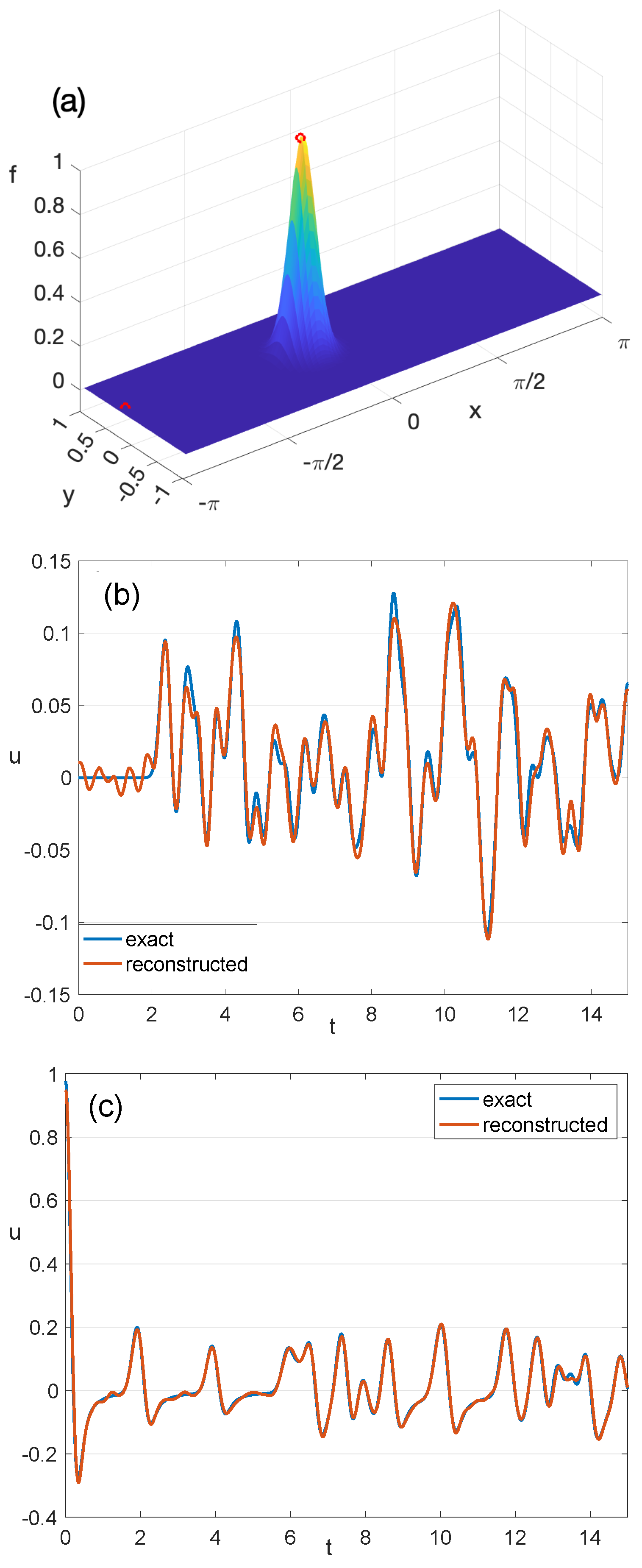
and a method such as ordinary least squares must be chosen to obtain an estimate of the coefficients ${\widehat{f}}_i$. This linear system can be written more succinctly as ${\alpha }_J={\Phi }_J{\widehat{f}}_J$. In practice, only finitely many eigenfunctions are of interest and the signals are bandlimited, but some eigenvalues will still correspond to many eigenfunctions. In Figure 1, least squares reconstruction is applied to the systems (25) for a two-dimensional case. The spatial domain is $\mathcal{D}=[0,\pi ]\times [0,1]$, and the boundary conditions are periodic. In the case of periodic boundary conditions, multiple sensors are always required because there are eigenvalues with a multiplicity greater than one, i.e., in one dimension:

$$\begin{array}{c}\hfill {\Phi }_n\left(x\right)=\sin (n\pi x/L)\mathrm{and}{\Phi }_{-n}\left(x\right)=\cos (n\pi x/L).\end{array}$$

(26)

In Figure 1, a network of seven sensors is used to construct approximations of the system. In the first panel, the initial state $f\left(\mathbf{x}\right)$ of the system, which is an off-center Gaussian bump, is displayed and the location of two additional sensors is shown in red. In the second and third panels of Figure 1, the time series of the two additional sensors are approximated. In both cases, the frequencies and amplitudes of the signal are recovered.

When the method of least squares is used, the error in the estimates ${\tilde{f}}_J$ of the coefficients ${\widehat{f}}_J$ can be written in terms of the matrix ${\Phi }_J$. Suppose the system is contaminated with Gaussian noise so that ${\alpha }_J={\Phi }_J{\widehat{f}}_J+{ϵ}_J$ where ${ϵ}_J\sim {\mathcal{N}}_n(0,{\sigma }^2{I}_n)$ for some $\sigma >0$. The best linear unbiased estimate ${\tilde{f}}_J$ of ${\widehat{f}}_J$ and its covariance are

$$\begin{array}{cc}\hfill {\tilde{f}}_J& ={\left({\Phi }_J^T{\Phi }_J\right)}^{-1}{\Phi }_J^T{\alpha }_J\hfill \end{array}$$

(27)

$$\begin{array}{cc}\hfill {\sigma }_J^2& =\mathbb{E}\left[({\tilde{f}}_J-{\widehat{f}}_J){({\tilde{f}}_J-{\widehat{f}}_J)}^T\right|{\Phi }_J]={\left({\Phi }_J^T{\Phi }_J\right)}^{-1}{\sigma }^2.\hfill \end{array}$$

(28)

To see how the error depends explicitly on the number of noisy sensors n in the network, the entries of the matrix ${\Phi }_J$ must be given a distribution. In the simplest case where $[{\Phi }_{i_1}\left({\mathbf{s}}_k\right),\dots ,{\Phi }_{i_{m_j}}\left({\mathbf{s}}_k\right)]$ is normally distributed $\mathcal{N}(0,\Sigma )$, then

$$\begin{array}{c}\hfill {\left({\Phi }_J^T{\Phi }_J\right)}^{-1}\sim {\mathcal{W}}_{m_j}^{-1}({\Sigma }^{-1},n)\end{array}$$

(29)

where ${\mathcal{W}}^{-1}$ denotes the inverse Wishart distribution. Alternatively, if the eigenfunctions are known, then a distribution is given to the sensor placement such as

$$\begin{array}{c}\hfill \mathbf{s}\sim \mathrm{Unif}\left(\mathcal{D}\right).\end{array}$$

(30)

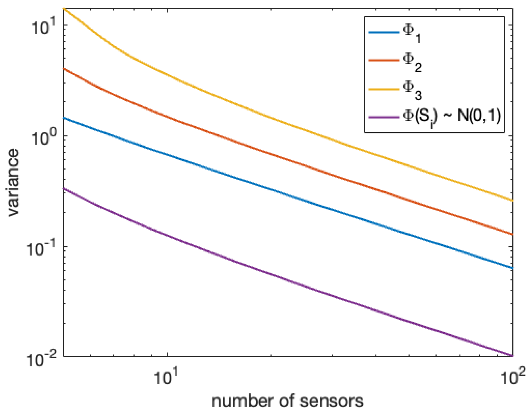
In Figure 2, the variance (28) is shown on a log–log plot for different distributions of ${\Phi }_i\left({\mathbf{s}}_k\right)$. For the first three, the sensor is placed uniformly at random in the domain, and the eigenfunctions

$$\begin{array}{cc}\hfill {\Phi }_1\left(x\right)=\sin \left(4x\right)& \mathcal{D}=[-\pi ,\pi ]\hfill \end{array}$$

(31)

$$\begin{array}{cc}\hfill {\Phi }_2\left(\mathbf{x}\right)=\sin \left(7x\right)\cos \left(12\pi y\right)& \mathcal{D}=[-\pi ,\pi ]\times [-1,1]\hfill \end{array}$$

(32)

$$\begin{array}{cc}\hfill {\Phi }_3\left(\mathbf{x}\right)=\cos \left(16x\right)\cos \left(23\pi y\right)\sin \left(28\pi z\right)& \mathcal{D}=[-\pi ,\pi ]\times [-1,1]\times [-1,1]\hfill \end{array}$$

(33)

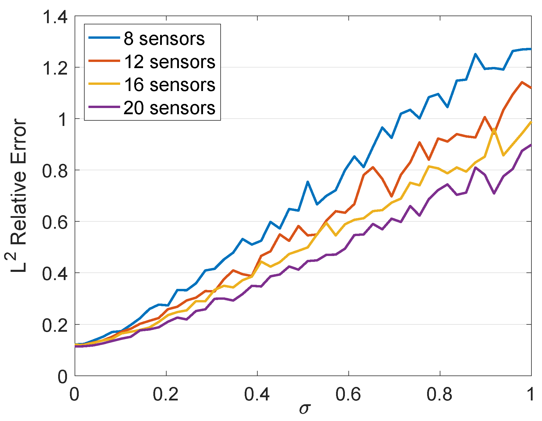
are used. The variance (28) is also plotted for the case where ${\Phi }_i\left({\mathbf{s}}_k\right)\sim \mathcal{N}(0,1)$. On this log–log plot, the slope of each line is approximately $-1$, meaning that the variance in each case decays as $\mathcal{O}\left(n^{-1}\right)$, where n is the number of sensors. Figure 3 shows how the relative error depends on the number of sensors and the noise level $\sigma$ of the sensors. In this figure, the error is the $L^2\left([0,100]\right)$ error in approximating the time series of an additional sensor.

4. 3D Stochastic Maxwell Vector Wave Equation and Optimal Observation Time

In this section, the signal processing of vectorial electromagnetic waves in the presence of a noisy current density $\mathbf{J}(\mathbf{x},t)$ is discussed (see [32], chapter 3). In this context, the medium parameters, permittivity $ϵ\left(\mathbf{x}\right)$ and permeability $\mu \left(\mathbf{x}\right)$, are general functions of space or are stratified and the current density is stochastic.

The electric field $\mathbf{E}$ satisfies the Maxwell vector wave equation:

$$\begin{array}{c}\hfill ϵ\left(\mathbf{x}\right)\frac{{\partial }^2\mathbf{E}}{\partial t^2}+\nabla \times \left({\left[\mu \left(\mathbf{x}\right)\right]}^{-1}\nabla \times \mathbf{E}\right)=-\frac{\partial \mathbf{J}}{\partial t}.\end{array}$$

(34)

The electric field solutions can be written in the form

$$\begin{array}{c}\hfill \mathbf{E}(\mathbf{x},t)=\sum _n{A}_n\left(t\right){\Phi }_n\left(\mathbf{x}\right)\end{array}$$

(35)

where $\Phi \left(\mathbf{x}\right)$ are eigenfunctions of the weighted curl-squared operator:

$$\begin{array}{c}\hfill \nabla \times \left({\left[\mu \left(\mathbf{x}\right)\right]}^{-1}\nabla \times \Phi \right)-\lambda ϵ\left(\mathbf{x}\right)\Phi =0.\end{array}$$

(36)

Stochasticity is introduced to the problem via the current density

$$\begin{array}{c}\hfill \frac{\partial \mathbf{J}}{\partial t}:=ϵ\left(\mathbf{x}\right)\sqrt{Q}\frac{\partial \mathcal{W}}{\partial t}\end{array}$$

(37)

where $\mathcal{W}$ is a cylindrical Wiener process and Q is a self-adjoint trace-class operator defined by $Q{\Phi }_n={\sigma }_n^2{\Phi }_n$ (see [33,34] for more details). The Wiener process $\sqrt{Q}\mathcal{W}$ can be written in terms of independent one-dimensional Wiener processes ${\mathcal{W}}_n\left(t\right)$:

$$\begin{array}{c}\hfill \sqrt{Q}\mathcal{W}=\sum _n{\sigma }_n{\mathcal{W}}_n\left(t\right){\Phi }_n\left(\mathbf{x}\right).\end{array}$$

(38)

Using the orthonormality of the eigenfunctions ${\Phi }_n\left(\mathbf{x}\right)$, a sequence of ODEs for the $A_n\left(t\right)$ terms is obtained:

$$\begin{array}{c}\hfill A_n^{″}\left(t\right)+{\lambda }_n{A}_n\left(t\right)={\sigma }_n\frac{\partial {\mathcal{W}}_n}{\partial t}\left(t\right).\end{array}$$

(39)

The solution is

$$A_n\left(t\right)={\widehat{f}}_n\cos \left(\sqrt{{\lambda }_n}t\right)+\frac{{\widehat{g}}_n}{\sqrt{{\lambda }_n}}\sin \left(\sqrt{{\lambda }_n}t\right)+{\int }_0^t\frac{{\sigma }_n}{\sqrt{{\lambda }_n}}\sin \left(\sqrt{{\lambda }_n}(t-r)\right)d{\mathcal{W}}_n\left(r\right)$$

and its variance grows linearly with time:

$$\begin{array}{c}\hfill \mathrm{VAR}\left[A_n\left(t\right)\right]=\frac{{\sigma }_n^2}{4{\lambda }_n^{3/2}}\left(2\sqrt{{\lambda }_n}t-\sin \left(2\sqrt{{\lambda }_n}t\right)\right).\end{array}$$

(40)

In the framework of the Maxwell vector wave equation, as in the last section, the inner products (21) can be utilized to reconstruct the electric field from sensor time series data; in this context, however, the time series data are bombarded with noise from the stochastic current density. Because the variance of the solution grows with time as a result of noise and a minimum-noise reconstruction is desired, sensor time series observed for a shorter time interval $[0,\tau ]$ can provide a better reconstruction of the noiseless electric field.

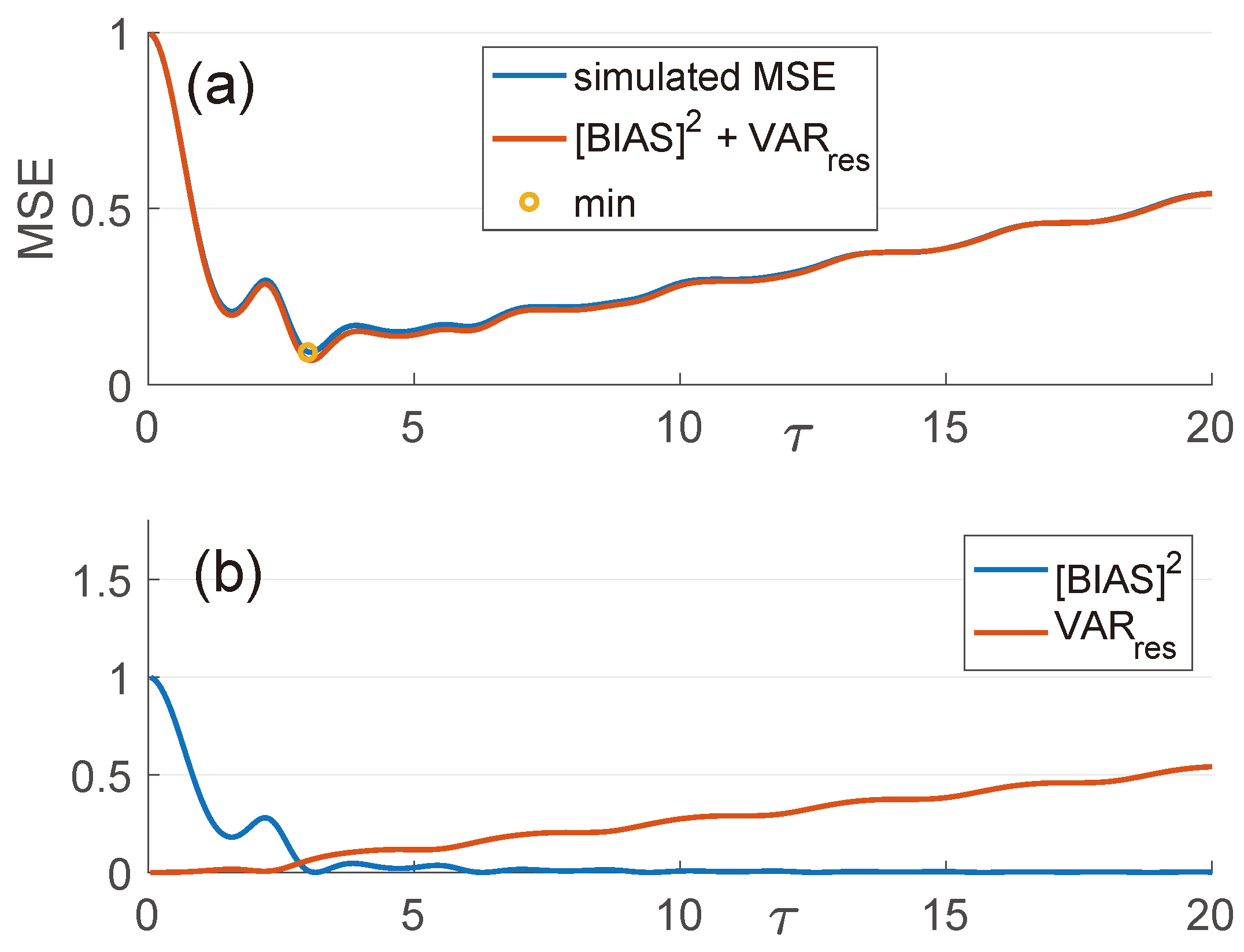
This can be made explicit by calculating the mean squared error (MSE) of each coefficient ${\widehat{f}}_j$ as a function of the sensor observation time $\tau$:

$$\begin{array}{c}\hfill \mathrm{MSE}(\tau ;j)={\left[\mathrm{BIAS}(\tau ;j)\right]}^2+\mathrm{VAR}(\tau ;j).\end{array}$$

(41)

The error resulting from the noisy current density is then described in terms of the variance term $\mathrm{VAR}$, and the deterministic error is described in terms of the squared-bias term ${\left[\mathrm{BIAS}\right]}^2$. The variance can be computed explicitly in simple cases and grows linearly with respect to the length of the time series $\tau$, i.e., $\mathrm{VAR}(\tau ;j)\sim \mathcal{O}\left(\tau \right)$. As a result, there is a bias–variance tradeoff. In Figure 4, the mean squared error of a coefficient ${\widehat{f}}_j$ is displayed. The MSE initially decreases as a result of the decreasing squared bias. After reaching a minimum, the MSE begins to grow roughly linearly as a result of the variance term. The observation time $\tau$ that minimizes the MSE is the “optimal” observation time. In Figure 4, the dominant variance term ${\mathrm{VAR}}_{\mathrm{res}}$ which can be calculated analytically is displayed along with the squared bias and MSE. This optimal observation time $\tau$ can be utilized to estimate each of the coefficients ${\widehat{f}}_j$ and reconstruct the electric field $\mathbf{E}$.

5. Concluding Remarks

In this review, we discussed recent advancements in the modeling and processing of vectorial electromagnetic signals propagating in inhomogeneous, stratified media. With new developments in vector sensor technology and the development of cheaper satellites, corresponding advancements in signal processing need to be made. The Maxwell vector wave equation, the governing equation for vectorial EM waves derived directly from Maxwell’s equations, incorporates relevant fundamental physics phenomena that are absent in scalar wave equation approaches. In applications involving EM wave propagation through media with sharp refractive index gradients, the modeling of vectorial effects is essential. Beyond the incorporation of vectorial effects, we reviewed new results on the importance of sensor networks for the accurate reconstruction of electromagnetic signals as well as modeling noisy environments via stochastic currents.

References

- Solar and Space Physics: A Science for a Technological Society; National Academies Press: Washington, DC, USA, 2013.
- Kak, A.; Akyildiz, I.F. Designing large-scale constellations for the Internet of Space Things with CubeSats. IEEE Internet Things J. 2020, 8, 1749–1768. [Google Scholar] [CrossRef]
- Lind, F.D.; Erickson, P.J.; Hecht, M.; Knapp, M.; Crew, G.; Volz, R.; Swoboda, J.; Robey, F.; Silver, M.; Fenn, A.J.; et al. AERO & VISTA: Demonstrating HF radio interferometry with vector sensors. In Proceedings of the 33rd Annual AIAA/USU Conference on Small Satellites, Logan, UT, USA, 20 August 2019. [Google Scholar]
- Knapp, M.; Robey, F.; Volz, R.; Lind, F.; Fenn, A.; Morris, A.; Silver, M.; Klein, S.; Seager, S. Vector antenna and maximum likelihood imaging for radio astronomy. In Proceedings of the 2016 IEEE Aerospace Conference, Big Sky, MT, USA, 5–12 March 2016; pp. 1–17. [Google Scholar]
- Loi, S.T.; Murphy, T.; Cairns, I.H.; Menk, F.W.; Waters, C.L.; Erickson, P.J.; Trott, C.M.; Hurley-Walker, N.; Morgan, J.; Lenc, E.; et al. Real-time imaging of density ducts between the plasmasphere and ionosphere. Geophys. Res. Lett. 2015, 42, 3707–3714. [Google Scholar] [CrossRef]
- Abarzhi, S.I. Review of theoretical modelling approaches of Rayleigh–Taylor instabilities and turbulent mixing. Philos. Trans. R. Soc. A Math. Phys. Eng. Sci. 2010, 368, 1809–1828. [Google Scholar] [CrossRef] [PubMed]
- Zhou, Y.; Williams, R.J.; Ramaprabhu, P.; Groom, M.; Thornber, B.; Hillier, A.; Mostert, W.; Rollin, B.; Balachandar, S.; Powell, P.D.; et al. Rayleigh–Taylor and Richtmyer–Meshkov instabilities: A journey through scales. Phys. D Nonlinear Phenom. 2021, 423, 132838. [Google Scholar] [CrossRef]
- Mahalov, A. Multiscale modeling and nested simulations of three-dimensional ionospheric plasmas: Rayleigh–Taylor turbulence and nonequilibrium layer dynamics at fine scales. Phys. Scr. 2014, 89, 098001. [Google Scholar] [CrossRef]
- Zhou, Y. Rayleigh–Taylor and Richtmyer–Meshkov instability induced flow, turbulence, and mixing. I. Phys. Rep. 2017, 720–722, 1–136. [Google Scholar]
- Tatarski, V.I. Wave Propagation in a Turbulent Medium; McGraw-Hill: Columbus, OH, USA, 1961. [Google Scholar]
- Immel, T.J.; Harding, B.J.; Heelis, R.A.; Maute, A.; Forbes, J.M.; England, S.L.; Mende, S.B.; Englert, C.R.; Stoneback, R.A.; Marr, K.; et al. Regulation of ionospheric plasma velocities by thermospheric winds. Nat. Geosci. 2021, 14, 893–898. [Google Scholar] [CrossRef] [PubMed]
- Sahba, S.; Sashidhar, D.; Wilcox, C.C.; McDaniel, A.; Brunton, S.L.; Kutz, J.N. Dynamic mode decomposition for aero-optic wavefront characterization. Opt. Eng. 2022, 61, 013105. [Google Scholar] [CrossRef]
- Tran, L. Strong Winds Power Electric Fields in the Upper Atmosphere, NASA’s ICON Finds. 2021. Available online: https://www.nasa.gov/feature/goddard/2021/strong-winds-power-electric-fields-in-upper-atmosphere-icon (accessed on 4 August 2023).
- Herring, J.; Kimura, Y. Some issues and problems of stably stratified turbulence. Phys. Scr. 2013, 2013, 014031. [Google Scholar] [CrossRef]
- Kimura, Y.; Herring, J. Energy spectra of stably stratified turbulence. J. Fluid Mech. 2012, 698, 19–50. [Google Scholar] [CrossRef]
- Herring, J. A Brief History of the Geophysical Turbulence Program at NCAR. In IUTAM Symposium on Developments in Geophysical Turbulence; Springer: Berlin/Heidelberg, Germany, 2000; pp. 1–4. [Google Scholar]
- Charbonneau, P.; Herring, J.; Milliff, R. Preface. Theoret. Comput. Fluid Dyn. 1998, 11, 137–138. [Google Scholar]
- Babin, A.; Mahalov, A.; Nicolaenko, B. On nonlinear baroclinic waves and adjustment of pancake dynamics. Theor. Comput. Fluid Dyn. 1998, 11, 215–235. [Google Scholar] [CrossRef]
- Mahalov, A. Turbulence and waves in the upper troposphere and lower stratosphere. In Aviation Turbulence: Processes, Detection, Prediction; Sharman, R., Lane, T., Eds.; Springer: Berlin/Heidelberg, Germany, 2016; pp. 407–424. [Google Scholar]
- Fernando, H.J.S. Turbulent mixing in stratified fluids. Annu. Rev. Fluid Mech. 1991, 23, 455–493. [Google Scholar] [CrossRef]
- Kelley, M.C. The Earth’s Ionosphere: Plasma Physics and Electrodynamics; Academic Press: Burlington, MA, USA, 2009. [Google Scholar]
- Cox, D. Depolarization of radio waves by atmospheric hydrometeors in earth-space paths: A review. Radio Sci. 1981, 16, 781–812. [Google Scholar] [CrossRef]
- Shaffer, S.R.; Mahalov, A. Permittivity gradient induced depolarization: Electromagnetic propagation with the Maxwell vector wave equation. IEEE Trans. Antennas Propag. 2020, 69, 1553–1559. [Google Scholar] [CrossRef]
- Wang, Q.; Alappattu, D.P.; Billingsley, S.; Blomquist, B.; Burkholder, R.J.; Christman, A.J.; Creegan, E.D.; De Paolo, T.; Eleuterio, D.P.; Fernando, H.J.S.; et al. CASPER: Coupled air–sea processes and electromagnetic ducting research. Bull. Am. Meteorol. Soc. 2018, 99, 1449–1471. [Google Scholar] [CrossRef]
- McDaniel, A.; Mahalov, A. Lensing effects in a random inhomogeneous medium. Opt. Express 2017, 25, 28157–28166. [Google Scholar] [CrossRef]
- McDaniel, A.; Mahalov, A. Coupling of paraxial and white-noise approximations of the Helmholtz equation in randomly layered media. Phys. D Nonlinear Phenom. 2020, 409, 132491. [Google Scholar] [CrossRef]
- McDaniel, A.; Mahalov, A. Stochastic mirage phenomenon in a random medium. Opt. Lett. 2017, 42, 2002–2005. [Google Scholar] [CrossRef]
- Mahalov, A.; McDaniel, A. Long-range propagation through inhomogeneous turbulent atmosphere: Analysis beyond phase screens. Phys. Scr. 2019, 94, 034003. [Google Scholar] [CrossRef]
- Barclay, B.M.; Kostelich, E.J.; Mahalov, A. Sensor Placement Sensitivity and Robust Reconstruction of Wave Dynamics from Multiple Sensors. SIAM J. Appl. Dyn. Syst. 2022, 21, 2297–2313. [Google Scholar] [CrossRef]
- Erichson, N.B.; Mathelin, L.; Kutz, J.N.; Brunton, S.L. Randomized dynamic mode decomposition. SIAM J. Appl. Dyn. Syst. 2019, 18, 1867–1891. [Google Scholar] [CrossRef]
- Hashemi, A.; Schaeffer, H.; Shi, R.; Topcu, U.; Tran, G.; Ward, R. Generalization bounds for sparse random feature expansions. Appl. Comput. Harmon. Anal. 2023, 62, 310–330. [Google Scholar] [CrossRef]
- Barclay, B. Stochastic Maxwell’s Equations: Robust Reconstruction of Wave Dynamics from Sensor Data and Optimal Observation Time. Ph.D. Thesis, Arizona State University, Tempe, AZ, USA, 2023. [Google Scholar]
- Da Prato, G.; Zabczyk, J. Stochastic Equations in Infinite Dimensions, 2nd ed.; Cambridge University Press: Cambridge, UK, 2014. [Google Scholar]
- Flandoli, F.; Mahalov, A. Stochastic three-dimensional rotating Navier–Stokes equations: Averaging, convergence and regularity. Arch. Ration. Mech. Anal. 2012, 205, 195–237. [Google Scholar] [CrossRef]
Figure 1.
Time series data from a network of seven sensors are used to approximate the wave field u by solving the systems (25). (a) The locations of an eighth and ninth sensor in red plotted on the initial state of the system (15). (b,c) Comparisons of time series of the eighth and ninth sensors to the reconstructions of the time series at those locations using the network of seven sensors.
Figure 2.
The variance of the least squares estimate (28) of a coefficient plotted against the number of sensors used. Each line displays the variance for a different assumption for how the data are obtained.
Figure 3.
The relative error in approximating the time series of a sensor plotted against the sensor noise level and the number of sensor time series used for approximation. The final time is .
Disclaimer/Publisher’s Note: The statements, opinions and data contained in all publications are solely those of the individual author(s) and contributor(s) and not of MDPI and/or the editor(s). MDPI and/or the editor(s) disclaim responsibility for any injury to people or property resulting from any ideas, methods, instructions or products referred to in the content. |
© 2023 by the authors. Licensee MDPI, Basel, Switzerland. This article is an open access article distributed under the terms and conditions of the Creative Commons Attribution (CC BY) license (https://creativecommons.org/licenses/by/4.0/).
Share and Cite
MDPI and ACS Style
Barclay, B.M.; Kostelich, E.J.; Mahalov, A. Vectorial EM Propagation Governed by the 3D Stochastic Maxwell Vector Wave Equation in Stratified Layers. Atmosphere 2023, 14, 1451. https://doi.org/10.3390/atmos14091451
AMA Style
Barclay BM, Kostelich EJ, Mahalov A. Vectorial EM Propagation Governed by the 3D Stochastic Maxwell Vector Wave Equation in Stratified Layers. Atmosphere. 2023; 14(9):1451. https://doi.org/10.3390/atmos14091451
Chicago/Turabian StyleBarclay, Bryce M., Eric J. Kostelich, and Alex Mahalov. 2023. "Vectorial EM Propagation Governed by the 3D Stochastic Maxwell Vector Wave Equation in Stratified Layers" Atmosphere 14, no. 9: 1451. https://doi.org/10.3390/atmos14091451
Note that from the first issue of 2016, this journal uses article numbers instead of page numbers. See further details here.