The Robustness of the Derived Design Life Levels of Heavy Precipitation Events in the Pre-Alpine Oberland Region of Southern Germany

Abstract

Extreme value analysis (EVA) is well-established to derive hydrometeorological design values for infrastructures that have to withstand extreme events. Since there is concern about increased extremes with higher hazard potential under climate change, alterations of EVA are introduced for which statistical properties are no longer assumed to be constant but vary over time. In this study, both stationary and non-stationary EVA models are used to derive design life levels (DLLs) of daily precipitation in the pre-alpine Oberland region of Southern Germany, an orographically complex region characterized by heavy precipitation events and climate change. As EVA is fraught with uncertainties, it is crucial to quantify its methodological impacts: two theoretical distributions (i.e., Generalized Extreme Value (GEV) and Generalized Pareto (GP) distribution), four different parameter estimation techniques (i.e., Maximum Likelihood Estimation (MLE), L-moments, Generalized Maximum Likelihood Estimation (GMLE), and Bayesian estimation method) are evaluated and compared. The study reveals large methodological uncertainties. Discrepancies due to the parameter estimation methods may reach up to 45% of the mean absolute value, while differences between stationary and non-stationary models are of the same magnitude (differences in DLLs up to 40%). For the end of this century in the Oberland region, there is no robust tendency towards increased extremes found.

1. Introduction

In 2021, several parts of the world were affected by severe flooding due to heavy precipitation. Particularly China, India, and Western Europe suffered many casualties and high financial losses (e.g., [1]). In July of the same year, Western Germany experienced exceptionally high rainfall rates of up to 200 mm from 13 to 15 July which exceeded the average monthly precipitation amounts, leading to the Ahrtal flood [2,3].

Often, when such weather extremes happen, questions regarding the possible impact of human-induced climate change arise, but only attribution studies may help to quantify the likelihood that specific events are a result of human influence [2]. However, the long-term impact of climate change on the evolution of extremes can very well be examined [2]. The latest reports of the Intergovernmental Panel on Climate Change (IPCC) identified increases in the frequency and intensity of extreme precipitation in the past and projected further enhancements in the future as likely (e.g., [4,5]). For example, a heavy precipitation event that happened approximately just once every ten years in a pre-industrial world (1850–1900) is now likely to occur more often with a frequency of 1.3 times in ten years [4]. In a future scenario with a 4 °C warmer world than in the pre-industrial state, corresponding to the high-impact emission scenario RCP8.5 [6], the aforementioned event is even more likely to occur with an average frequency of 2.7 times in the same period of time [4]. This is in line with the thermodynamic law of Clausius–Clapeyron, according to which atmospheric moisture content exponentially increases with warmer temperatures resulting in higher precipitable water [4,7] and therefore in enhanced precipitation intensities if moisture availability is not a limiting factor [4,8].

A consequence of increased extreme precipitation would be a greater probability of flooding at regional scales, especially in mountainous and urban areas [4]. Hence, flood protection is an important topic in regions that are prone to flood hazards through heavy precipitation, and new challenges regarding ongoing climate change require improved adaptation measures. To design protection measures appropriately, design values (commonly referred to as return levels (RL)) are calculated, which the structure must withstand [9,10,11].

Up to now, the best available approach to estimate RLs is the extreme value analysis (EVA) [12], which aims to describe the stochastic behavior of a process at unusually high (or low) levels and hence makes presumptions about probable extreme levels in a certain future time period [12].

Practically, EVA is applied to estimate the stochastic behavior of a process at more extreme levels than already observed [12,13]. This extrapolation to more extreme (i.e., less likely) events is achieved by fitting a theoretical distribution function ($df$) to the selected subset of extremes and deriving a value which—according to this $df$—would occur with a certain small probability [9,12]. The accurate estimation of these tails is in general challenging since there is usually only little data available to fit the theoretical model to the sample of the extreme values [12].

For the selection of the extreme values from the observed time series, two different approaches are commonly in use: (i) the peaks over threshold (POT), where extreme values above a selected threshold are selected for the EVA; (ii) the block maxima (BM) approach, where extreme values of a certain period are selected. Often, annual maximum (AMAX) values are selected as BM. Compared to the AMAX, the sample size of the POT approach can be increased by lowering the threshold value, which might possibly lead to an improvement of estimation of design life levels using POT [10,12,14]. An appropriate threshold should, on the one hand, be high enough to minimize the bias due to the asymptotic tail approximation, and, on the other hand, be low enough to obtain a sufficient sample size in order to keep parameter estimation uncertainties as low as possible [10,15,16]. Scarrott and Macdonald [15] provided a comprehensive review on threshold value selection. POT is also recommended for relatively short time series or time series with the infrequent occurrence of extremes and requires higher resolution of the basic time series, i.e., hourly or daily observations [10,12,17].

Two generalized theoretical distribution functions exist which can be fitted to the derived extreme values, i.e., based on AMAX and POT. Firstly, following the AMAX approach, the distribution of annual extremes (AMAX) converges to the Generalized Extreme Value (GEV) distribution. The GEV combines three limiting distribution functions, namely Gumbel, Fréchet, and Weibull, into one family [18,19]. Secondly, following the POT approach, the generalized Pareto distribution (GP) is considered an appropriate theoretical distribution [12,14]. The parameters of the theoretical distribution functions can be fitted by different parameter estimation methods (PEMs). Well-established fitting procedures are, amongst others, the Maximum Likelihood Estimation (MLE) (e.g., [12]), the L-moments (e.g., [10]), the Generalized Maximum Likelihood Estimation (GMLE) (e.g., [20]), and the Bayesian approach (e.g., [21]). The choice of a suitable PEM strongly depends on the sample size (e.g., [12]). A more thorough discussion on the impact of the fitting procedure is given in Section 2.3.2.

Consequently, the selection of the different theoretical distribution functions for extremes, parameter estimation methods, and approaches for the selection of the extreme values from a time series can finally result in large uncertainties of derived design life levels, particularly at low occurrence probabilities [22]. Since the presence or absence of individual extreme events of existing time series can confound the statistical representativeness of that time series for the corresponding region, a comprehensive database is necessary to reliably assess the return periods (RP) of the extreme values. In practice, this is often a limitation and becomes even more important the higher the assumed return level is.

However, even if the time series well represents the historical period, it is not necessarily representative of the future. One of the most frequently discussed topics is the lack of a possibility to capture changes in extremal behavior with traditional EVA [10,23,24]. If extremes tend to become more likely to occur, a return period of an event from an earlier period can thus be much larger than that of the same event in a later period. This also has practical implications for engineering practice such as in hydrodynamic modeling based on heavy precipitation events to derive inundation maps and flood protection measures in the end [25].

With traditional EVAm, such changes in extremes cannot be considered since only one return level is calculated representing the whole time series. Therefore, the question arises whether traditional methods are still adequate or whether new statistical methods should be developed to account for potential changes in (future) extremes. Hence, many studies applied a new concept referred to as non-stationary extreme value analysis (non-stationary EVA). In contrast to traditional (i.e., stationary) EVA, it is assumed that the statistical properties of time series change, which enables the consideration of alterations in extremes through climate change or—especially in the context of flooding—other (human) interventions such as land cover change, urbanization, or river regulation [11,26].

Following the definition of stationarity of Coles [12], in a non-stationary time series, the properties of the distribution function are enabled to shift over time. These changes can emerge in different ways, such as adding a linear link function relating the distribution parameters to explanatory variables [19,27,28,29], or more complex structures such as cubic splines [23] or quadratic trends [30]. Nevertheless, although published studies demonstrate shifts in both mean and extreme values of precipitation, evapotranspiration, and river discharge rates [4], consensus remains elusive regarding the utilization of non-stationary EVA relationships [10,11]. Since it is virtually impossible to know the true underlying statistical characteristics of hydrometeorological time series [12], there is often no plain distinction between whether a times series can be called stationary or non-stationary. Random fluctuations or deviations from the mean are to be expected even in stationary time series [31], and the sample can also be part of a cyclical climate variability [32]. Therefore, the future state may be stationary but just different from the one before [33,34]. Matalas [33] considers extrapolating the continuation of non-stationarity in the form of a trend into the future to be problematic. This uncertainty arises from the question of whether an observed trend in the past genuinely signifies non-stationarity [31,33,35], and thus whether it can be extended into the future without resulting in ‘catastrophic consequences’. Hence, several studies recommend the use of the non-stationarity assumption only when changes can be predicted due to the knowledge of underlying physical drivers [22,35].

In case non-stationary EVA is applied inappropriately (especially to short time series), this may increase the uncertainties, and thus stationary EVA should be better used by default [22]. Furthermore, there is also no agreement on the methodology of non-stationary EVA [10]. This is mainly because typical concepts of return period and return level no longer provide distinct values in the non-stationary case [28,36]. Alternative concepts have been developed such as the design life levels (DLLs) and minmax design life levels from [27], the approaches of expected waiting time until a given exceedance occurs, or the expected number of events over the return period [28] as well as equivalent reliability by Hu et al. [37].

In this study, one stationary and three non-stationary statistical models are checked for their robustness in deriving DLLs of precipitation extremes. In order to allow for a direct comparison between stationary and non-stationary methods, a rather simple but effective approach based on the concept of DLLs is developed. For the assessment under stationary (non-stationary) conditions, method-inherent uncertainties are quantified by using two (one) theoretical extreme value distribution(s), and four (three) parameter estimation methods. It is expected that a quantification of the method-inherent uncertainties under current climate conditions allows a more robust assessment of precipitation extremes under future climate conditions. Moreover, it is analyzed how regional climate models (RCMs) can be used to derive future DLLs. The results are compared to the results of the non-stationary statistical models using extrapolated observations for the future.

2. Materials and Methods

This section introduces the study region, the used data, and the methodologies applied in this study.

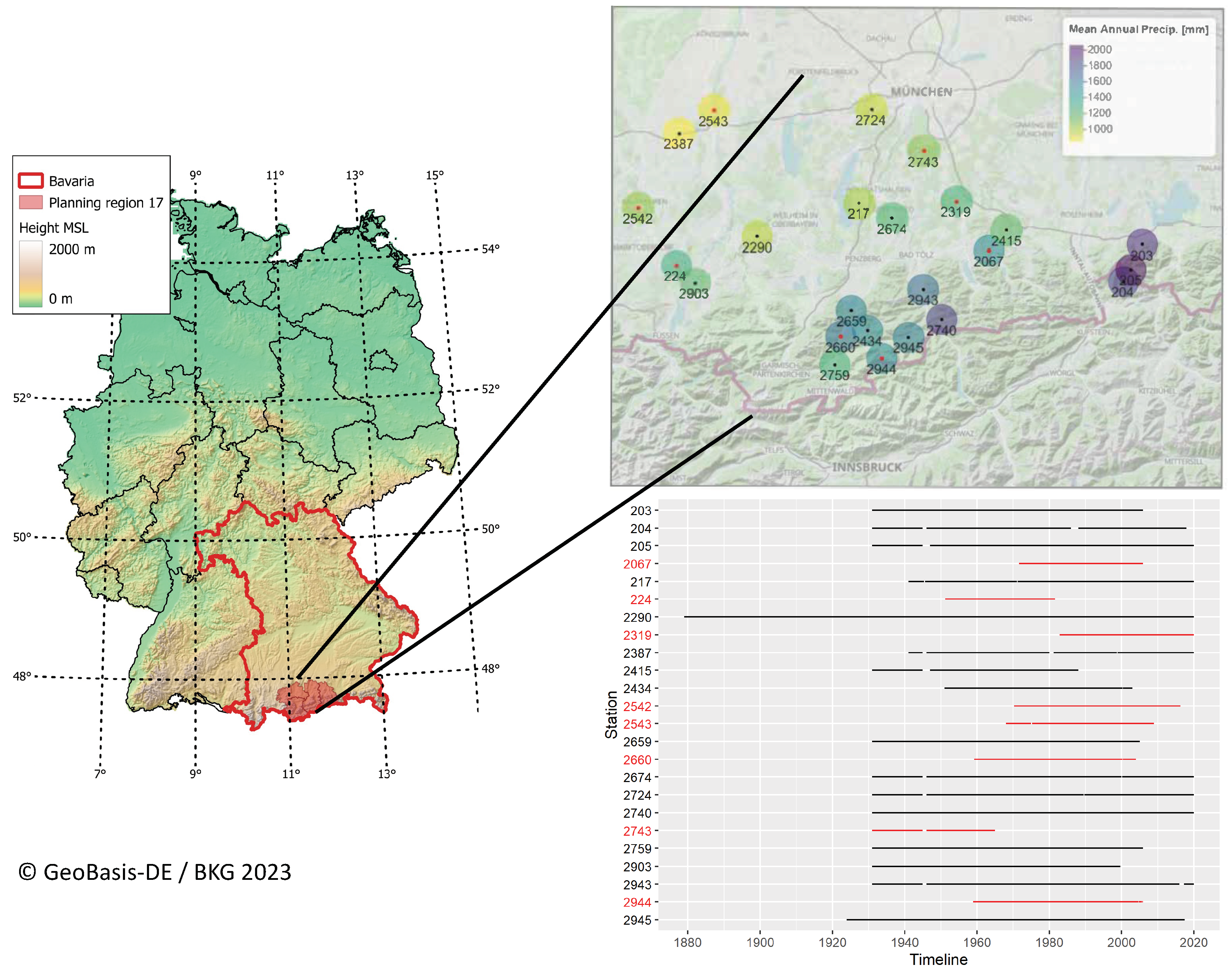
2.1. Study Region

The study area mainly comprises the Oberland region of the federal state Bavaria in the south of Germany (Figure 1). More precisely, the Oberland region includes the districts Bad Tölz-Wolfratshausen, Garmisch-Partenkirchen, Miesbach, and Weilheim-Schongau. The topography of the study area is characterized by the flatter alpine foothills in the north of the region and alpine areas in the south. Following the elevation gradient in the study region, the distribution of precipitation reveals higher mean annual sums in the south than the north [38]. Besides the annual amounts, extreme precipitation events can occur due to different prevailing weather situations in the region, mainly due to the blockage of northerly flows of humid air masses at the northern edge of the Alps, often referred to as the so-called Vb-cyclones [39], and due to deep convection, partly triggered by the mountainous terrain of the Alps [40].

Moreover, it has been shown that the precipitation patterns have undergone significant changes, most likely due to global climate change [38]. Thus, although the Oberland region comprises a relatively small region (in Germany), it may serve as a blueprint for larger regions with complex orography, complex precipitation regimes, and regions that are already affected by climate change.

2.2. Data

Across the study area, there are 24 observation stations available with sufficiently long time series of daily precipitation data, i.e., a minimum of 30 years is required for EVA of 100-year return periods. However, as it requires a very long time series to investigate possible changes in statistical characteristics for non-stationary EVA [22,41], even stations with less than 50 years were neglected, which resulted in a total of 16 stations. For stationary EVA, all 24 stations were explicitly taken into consideration because one of the objectives is to demonstrate how the applied methods perform in relation to the length of the time series. Figure 1 shows the spatial distribution as well as the length of the observed time series of those 24 stations. Stations with less than 50 years of data are marked with red dots. A total of 16 stations have time series longer than 50 years and 13 stations have time series longer than 70 years. Data quality checks were performed by the German Weather Service (DWD). In this study, the annual extreme values were re-checked for plausibility. Based on the documented quality (meta-data) of the DWD as well as our own checks, the observations of all applied stations were considered fully plausible.

Besides station data, high-resolution RCM model simulations were used in this study to derive return levels (see

Table 1. Overview of utilized GCM-RCM combinations from EURO-CORDEX.

Driving Model (GCM)	RCM	Ensemble	${\mathit{T}}_{\mathit{h}}$	${\mathit{T}}_{\mathit{p}}$
ICHEC-EC-Earth	COSMO-crCLIM-v1-1	r1i1p1	1950–2005	2006–2100
ICHEC-EC-Earth	COSMO-crCLIM-v1-1	r3i1p1	1950–2005	2006–2100
ICHEC-EC-Earth	COSMO-crCLIM-v1-1	r12i1p1	1950–2005	2006–2100
MPI-M-MPI-ESM-LR	COSMO-crCLIM-v1-1	r1i1p1	1949–2005	2006–2100
MPI-M-MPI-ESM-LR	COSMO-crCLIM-v1-1	r2i1p1	1949–2005	2006–2100
MPI-M-MPI-ESM-LR	COSMO-crCLIM-v1-1	r3i1p1	1949–2005	2006–2100
CNRM-CERFACES-CNRM-CM5	COSMO-crCLIM-v1-1	r1i1p1	1951–2005	2006–2100

). In particular, outputs from Coordinated Downscaling Experiment—European Domain (EURO-CORDEX) at a horizontal grid spacing of 0.11° (EUR-11, approx. 12 km) were applied [42,43]. Due to computational resources, we restricted our analysis to CORDEX experiments based on the regional model COSMO-CLM, nested into three different general circulation models (GCMs) from the Coupled Model Intercomparison Project Phase 5 (CMIP5) [44]. Those are the EC-Earth from EC-Earth Consortium Europe, the CNRM-Cerfacs from the Centre National de Recherches Météorologiques, and the MPI-ESM-LR from the Max-Planck-Institute for Meteorology. Three realizations were available for MPI-ESM-LR (r1, r2, r3) and EC-Earth (r1, r3, r12), which only differ in their initial conditions [45,46]. Each future scenario simulation is assigned the same realization integer as the historical run from which it was initiated [46]. For future scenarios, the high-emission scenario RCP8.5 with 8.5 W/m${}^2$ radiative forcing in 2100 was chosen.

As can be seen from Table 1, historical simulations $\left(T_h\right)$ are available for approximately the period of 1950–2005 and future projections $\left(T_p\right)$ for the period of 2006–2100. Since an initial comparison of statistical properties with the observations is needed, local information from the climate data for the position of the above-mentioned stations is assessed. Therefore, the time series of the grid cells corresponding to the location of the stations were extracted. It is noteworthy that the utilized RCM simulations were bias-corrected [47] for specific EVA models (i.e., N2 and N3). For other assessments, only the (relative) climate change signal was needed rather than the intensity-corrected time series. In these cases, the delta change approach was followed.

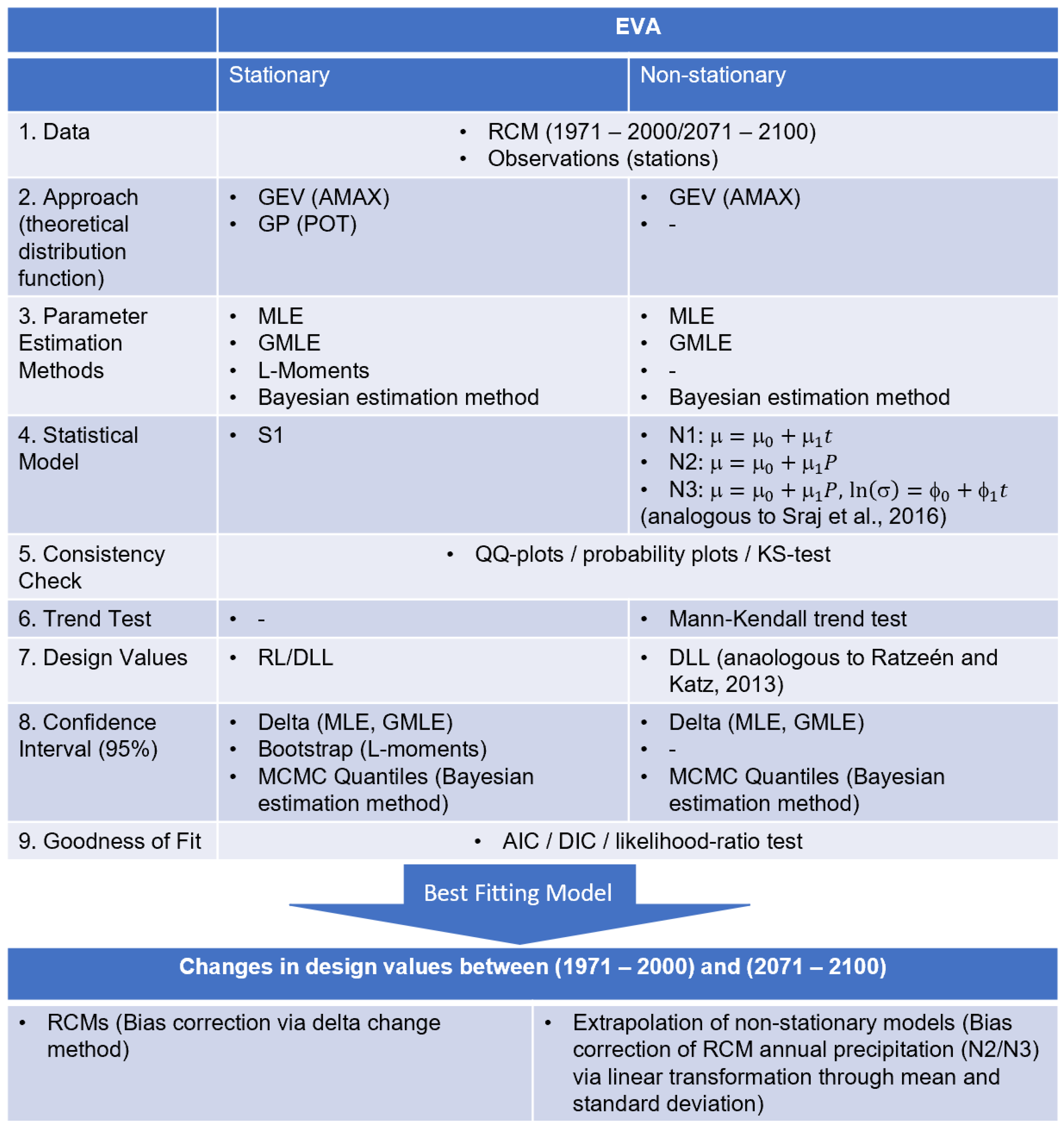
2.3. Methods

The Section 2.3 is subdivided into Theoretical Extreme Distribution Functions, Parameter Estimation Methods (PEMs), Goodness-of-Fit, followed by the description of the non-stationary models (Implementation of Non-Stationarity), considerations of the applied concept of Equivalent Design Life Level, and Usage of Regional Climate Models. Figure 2 provides a brief overview of the data and the applied methodologies in greater detail. It may serve as a guide through the workflow of both the stationary and the non-stationary EVA.

2.3.1. Theoretical Extreme Distribution Functions

In this study, we applied two theoretical distribution functions. Firstly, we utilized the Generalized Extreme Value (GEV) distribution based on AMAX. The cumulative distribution function of the GEV is expressed as follows:

$$F(x,\theta )=exp\left\{-{\left(1+\xi \left(\frac{x-\mu }{\sigma }\right)\right)}^{\frac{-1}{\xi }}\right\},\left(1+\xi \left(\frac{x-\mu }{\sigma }\right)\right)>0.$$

The function depends on three distribution parameters $\theta =(\mu ,\sigma ,\xi )$ which allows the flexibility to model different characteristics of extremes: the first one is the location parameter $\left(\mu \right)$ indicating the center of the distribution, the second is the scale parameter $\left(\sigma \right)$ representing the size of deviations around the location parameter, and the third is the shape parameter $\left(\xi \right)$ which controls the tail of the distribution function [12,19]. Just as the GEV remains an appropriate model for the AMAX, for a large enough threshold u, similar arguments suggest that the generalized Pareto distribution (GP) is appropriate for the selected threshold excesses [12,14]. The cumulative distribution function can be expressed as follows [12,48]:

$$F(x,\theta )=1-{\left(1+\frac{\xi (x-u)}{\tilde{\sigma }}\right)}^{\frac{-1}{\xi }},$$

$$\mathrm{where}(x-u)>0,\left(1+\frac{\xi (x-u)}{\tilde{\sigma }}\right)>0,\tilde{\sigma }>0.$$

There is a relationship between the GEV and GP distribution where the GP $df$ is approximately the tail of the GEV $df$ [12,49]. The scale parameter of the GP $df$$\tilde{\sigma }$ is a function of the parameters of the corresponding GEV $df$: $\tilde{\sigma }=\sigma +\xi (u-\mu )$. The shape parameter $\xi$ of the GP distribution is equivalent to that of the corresponding GEV distribution [14], which makes $\xi$ invariant to block size, while $\tilde{\sigma }$ is unperturbed by the changes in $\mu$ and $\sigma$ which are self-compensating [12]. Just as the shape parameter $\xi$ is dominant in determining the qualitative behavior of the GEV $df$, it is analogous for the GP $df$ [12].

To define a suitable threshold for the POT in this study, the 99th percentile of all rain day amounts was calculated for all stations [14,50]. This value was used and adjusted if the resulting sample size did not lie within the range of one to two times the length of the AMAX sample size [50]. In addition, since extremes over a threshold tend to cluster and thus induce serial dependence [12], a declustering approach was applied following Coles [12].

2.3.2. Parameter Estimation Methods (PEMs)

In this section, a short review of the four applied parameter estimation methods (PEMs) is given. Therefore, the Bayesian inference is described in greater detail since it is relatively new.

Maximum Likelihood Estimation (MLE)

The MLE approach became one of the standards in statistical inference because of its asymptotic efficiency with sample size n increasing to infinity and for distributions satisfying several regularity conditions [12,21,51]. As a likelihood-based approach, it tries to find the parameter values of $\theta$ which maximize the probability of resampling the data [9]. Meanwhile, it is one of the most frequently applied methods to estimate unknown parameters and, in addition, one of the most flexible regarding its application to modified models [12].

For the AMAX approach, it tends to become unstable for sample sizes of $n<50$ Coles and Dixon [52].

Method of Moments

A commonly employed variation of the method of moments is the L-moments method [10]. It is considered more robust to outliers and enables more secure inferences about the underlying probability distribution to be made from small samples [53]. For detailed information, Hosking [53] unified the theory of L-moments and provided guidelines for practical use.

For the GP, Hosking and Wallis [54] showed that unless the sample size is 500 or more, estimators derived by the method of moments are more reliable than those derived by MLE.

Generalized Maximum Likelihood Estimation (GMLE)

Another method to circumvent possible weaknesses of the MLE is the GMLE [20], which restricts the estimates of the shape parameter $\xi$. Since maximum likelihood estimates can generate absurd values of the GEV shape parameter $\xi$, when sample sizes are small [20,53], with GMLE, a prior distribution $\pi \left(\xi \right)$ is chosen, assigning weights to different values of $\xi$ within the allowed range. The choice of prior function is by default the beta distribution similar to that of Martins and Stedinger [17,20]. Analogous to the MLE method, the estimator of $\theta$ can be identified by maximizing the generalized log-likelihood function [20] which is the joint distribution of the likelihood function and the prior distribution.

Bayesian Inference

As an alternative to classical statistical inference, the last estimation technique used is based on Bayesian inference [21]. One of the main differences is that the parameters are no longer assumed to be constant but are rather treated as random variables with distribution function $f\left(\theta \right)$ [12]. This $df$ is called prior distribution since it contains possible beliefs about $\theta$ without reference to the data [12]. An obvious advantage of this method would be the inclusion of additional knowledge about the parameters which may come from other data sets or a modeler’s experience [21]. By applying the well-known Bayesian Theorem, the prior distribution can be converted into a posterior distribution $f\left(\theta \right|x)$, which includes the additional information provided by data x, as follows:

$$f\left(\theta \right|x)=\frac{f\left(\theta \right)f\left(x\right|\theta )}{\underset{\mathsf{\Theta }}{\int }f\left(\theta \right)f\left(x\right|\theta )d\theta }.$$

However, the normalization integral in the denominator complicates the direct computation of the posterior distribution [12,13]. This difficulty was overcome by the development of simulation-based techniques, such as Markov Chain Monte Carlo (MCMC), which facilitated the use of Bayesian techniques to the extent that they are now standard in many areas of application [12].

2.3.3. Goodness-of-Fit Test

After fitting the statistical models, the correspondence between modeled and the sample distribution was checked using numerous statistics such as quantile–quantile plots (QQ Plots), probability plots, and simple comparisons of density distributions as well as the Kolmogorov–Smirnov test (KS test) as a goodness-of-fit test [14,19,24,29].

2.3.4. Implementation of Non-Stationarity

In this study, non-stationarity was considered only for the AMAX approach and the MLE, GMLE, and Bayesian estimation methods. To check whether there is a justification for non-stationary assumptions, time series were checked first for trends. For most stations, a linear trend of the extremes (explored for annual maxima) provided a reasonable fit. It was noted that a linear trend did not always provide the best fit for all stations and strongly depended also on the observation period (length). Assuming a linear trend for the future, if no better-qualified assumptions exist, it is considered useful as a starting point [23,27]. Therefore, only linear dependencies for the location and scale parameter were included, as the estimation of the shape parameter is already, under stationary assumptions, the most difficult one and requires long-term observations that are in practice often not available (e.g., [12,19,29,36]). As suggested by many studies, the logarithm of the scale parameter was used to ensure positive values [29,36]. In addition to the stationary model S1, the following three non-stationary models were implemented:

• N1: non-stationary model (1) with location parameter $\mu$ being a function of time: $\mu$ (t) = ${\mu }_0$ + ${\mu }_1$ t;
• N2: non-stationary model (2) with location parameter $\mu$ being a function of annual precipitation: $\mu$(t) = ${\mu }_0$ + ${\mu }_1$ P;
• N3: non-stationary model (3) with location parameter $\mu$ being a function of annual precipitation and $\sigma$ parameter being a function of time: $\mu$(t) = ${\mu }_0$ + ${\mu }_1$ P, ln($\sigma$(t)) = ${\varphi }_0$ + ${\varphi }_1$ t.

These non-stationary models were adapted from Šraj et al. [29], but slightly changed for model N3 not only being dependent on time but rather a mixture of precipitation and time. Time as a covariate should be treated with caution because changes in the past are not automatically the same as in the future, especially for periods longer than ten years into the future [29]. An advantage of employing climate variables such as annual precipitation as a covariate is that climate model predictions or projections (see Section 2.3.6) can then be employed as covariates to estimate future change which makes the proposed model more practically useful [11,29]. As recommended by Gilleland and Katz [49], covariate vectors (time and precipitation) were scaled to zero (zero mean).

Detailed exploratory data analyses such as trend analyses are required particularly for the non-stationary EVA as existing trends can have a considerable effect on the results and their interpretation [22,29]. To check whether the inclusion of the certain covariate into the model was significant and to indicate the best fitting statistical model, the Akaike information criterion (AIC) and the deviance information criterion (DIC) were applied for MLE/GMLE and the Bayesian estimation method, respectively [29]. In both cases, models with the smallest AIC/DIC value indicate the best model performance [55]. In addition, for MLE and GMLE, a likelihood-ratio test (lr-test) was performed to test the significance of the inclusion of covariates into the models [29].

2.3.5. Equivalent Design Life Level

Since for non-stationary EVA the term return level becomes ambiguous, the concept of design life levels (DLL) by [27] was used and further developed as equivalent DLLs. This does not only allow a direct comparison between stationary and non-stationary EVA results, but is also considered more comprehensive and useful in applications compared to the concept of return levels since actual precipitation values are provided. Below, DLLs and equivalent DLLs are used synonymously.

Since the DLL is defined by the risk of exceedance in a certain time span, a connection between DLL and RL can be established through the common term of hydrological risk. For an n-year RL, the hydrological risk can be computed for the same time period as used at the computation of DLL and by equating the risks, an equivalent DLL can be computed that has the same risk of exceedance as the associated RL.

For a 10-year level and a time period of 30 years, the hydrological risk R would be $R=1-{(1-1⁄10)}^{30}=0.96$, and analogously for a 100-year level $R=1-{(1-1⁄100)}^{30}=0.26$. In this study, historical DLLs were computed for the time period of 1971–2000 and future DLLs were computed for 2071–2100.

Extrapolation of non-stationary models, i.e., models N2 and N3, requires a vector of the covariate in this future time period. For time as a covariate, this is a trivial derivation, but for annual precipitation as a covariate, climate model projections are necessary. Due to the partly strong deviations between modeled and observed annual precipitation in the RCM projections, the RCM annual precipitation was adjusted by using a linear transformation of the mean and the standard deviation between historical model simulations $x_{h,i}$ and observations $y_i$. Applying them to the future model simulations $x_{f,i}$, transformed future simulations $x_{ft,i}$ were then derived as follows:

$$x_{ft,i}=\frac{x_{f,i}-{\overline{x}}_f}{s_{x_f}}{s}_y+\overline{y}+({\overline{x}}_f-{\overline{x}}_h).$$

2.3.6. Usage of Regional Climate Models

RCMs potentially provide an opportunity for EVA in the absence of (sufficient) observation data, regarding not only the length of the time series but also their spatial distribution. In this context, we explored the general usability of RCMs by comparing the EVA results to those based on the observations. Firstly, the regional climate data were validated by comparing the distributions of precipitation from the observation stations to those of the corresponding RCM grid cells. Therefore, different approaches were followed, such as the visual inspection of boxplots (and especially deviations in the median) as well as Kolmogorov–Smirnov (KS) tests to compare the distributions of modeled and measured AMAX. Besides the extrapolation of DLLs from observations into the future (see models N2 and N3), climate models provide an additional possibility to derive information about future extreme behavior. Since RCM simulations used in this study were not bias-corrected per se (only for N2 and N3), projected DLLs were calculated with a simple and frequently used approach called the delta change method (e.g., [56,57,58,59]). It differs from other bias correction methods as it does not adjust RCM simulations itself but uses the combination of observations and only the RCM change signal [58,59]. In that way, differences, i.e., the change factor or the ‘delta’ between the design life level of the future $DL{L}_f$ (2071–2100) and historical simulations $DL{L}_h$ (1971–2000) were calculated and then added onto design life levels from observations DLL_obs.

It has to be mentioned that confidence intervals of the delta approach are symmetric, which does not represent the asymmetry that is generally associated with quantile estimators of extremes [36]. Since this approach is not always physically consistent and can attain negative values for the lower limit, it should be interpreted with caution [22].

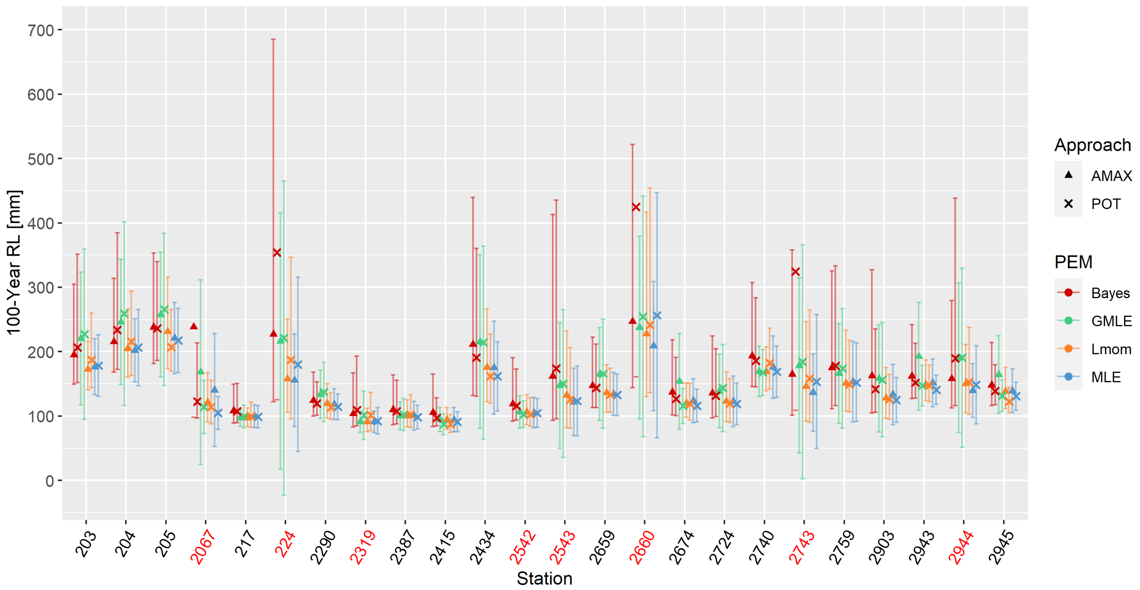
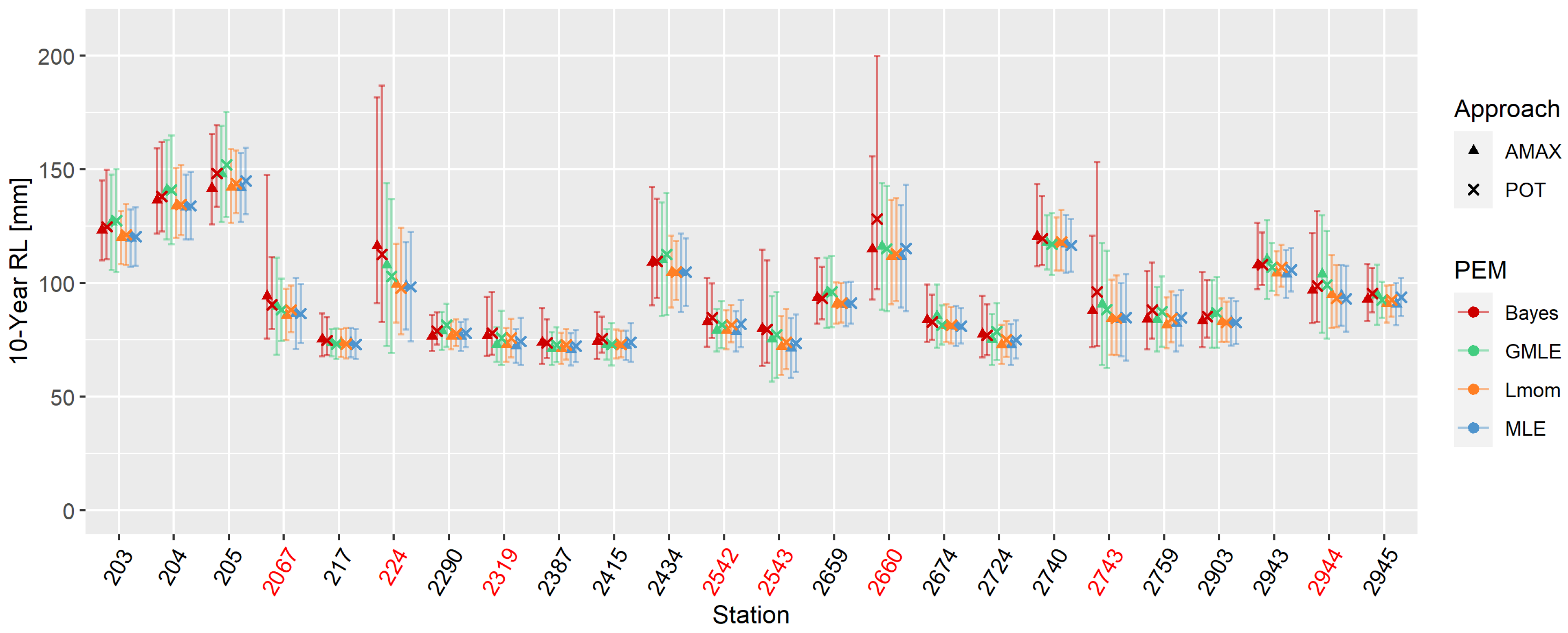
3. Results

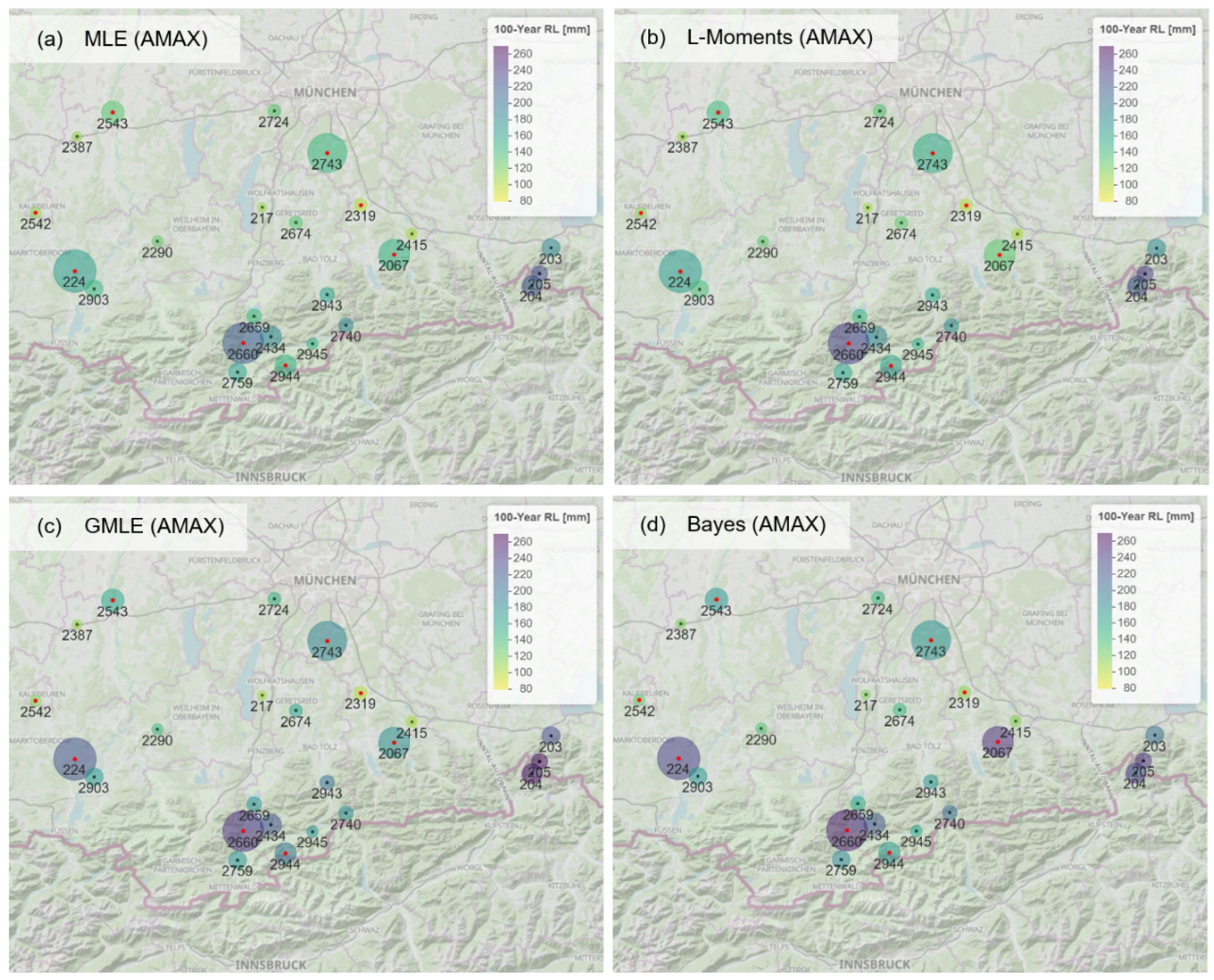
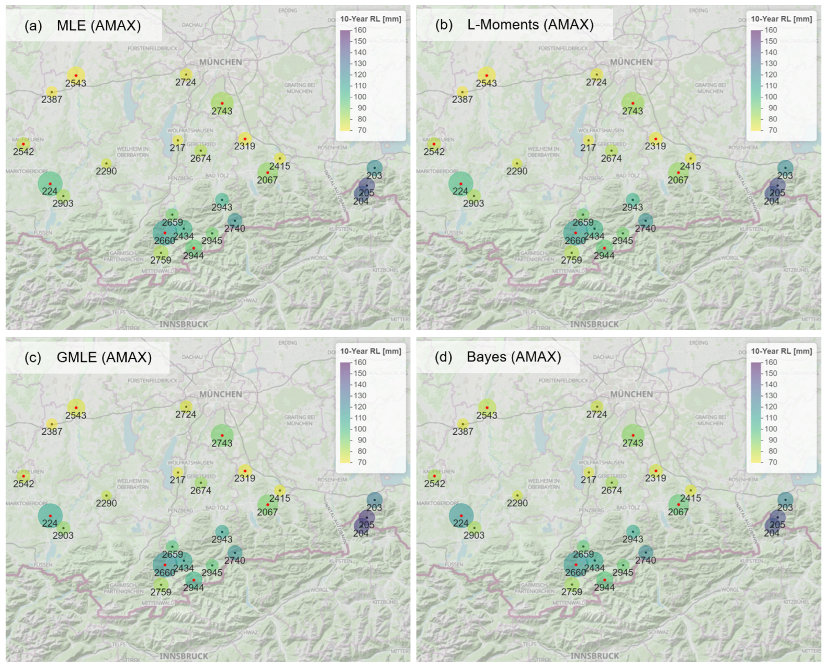
3.1. Theoretical Distributions and Parameter Estimation Methods

After modeling the extreme behavior using the GEV and GP distributions, the fit of the estimated models was evaluated for the observation stations in the Oberland region. It was found that only for a few stations the modeled distribution did not fit the data well. In particular, for station 2759, all estimated GEV models showed poor performance of the fitting based on KS tests. This was confirmed by visual inspection of the applied quantile–quantile (QQ) plots. For stations 2724 and 2903, the model fit was poor (underestimation of the occurrences of extreme events) when using the GEV distribution and GMLE and Bayesian estimation. These stations should therefore be interpreted with care in the following sections.

In the next step, parameter estimates were examined in greater detail with regard to the four estimation methods, i.e., MLE, GMLE, L-moments, and the Bayesian estimation method. Relative differences between the estimation methods were the largest for the shape parameter. In the case of AMAX, the variation coefficients of the shape parameter compared to those of the location parameter were approximately 50 times larger, and compared to POT variation coefficients, they were about 20 times larger than for the scale parameter. Generally highest values of $\left|\xi \right|$ were mostly obtained with GMLE, but also with the Bayesian estimation method. Curiously, GMLE estimates equaled estimates using L-moments if the shape parameter was negative.

For location and scale parameters, there was no discernible relation between estimation methods and parameters, but for AMAX, the Bayesian estimation method seemed to result in higher values as well. This behavior was reflected in the later derived RL. Figure 3 shows 100-year RLs for all stations with an indication of 95% confidence intervals. Again, stations with less than 50 years of data are indicated in red.

For stations 2067, 224, 2660, and 2743, the uncertainty ranges for some Bayesian estimates were too high to be illustrated properly, and thus omitted from the figure. Through those 24 stations, the range of RLs reached relatively low values of about 100 mm at stations 217, 2319, 2387, and 2415, to relatively high values between 150 and 270 mm at stations 203, 204, 205, 224, 2434, 2660 and 2740. Some stations show huge discrepancies between the different PEMs and modeling approaches with large uncertainties (especially stations 224, 2434, 2543, 2660, 2743, 2944). Others, in turn, had a good agreement on RLs (e.g., 217, 2290, 2319, 2387, 2415, 2542, 2659, 2674, 2724, 2740, 2943, 2945). Of the former, a large proportion had time series shorter than 50 years, but there were also stations with short time series that have small uncertainties and strong agreement between different RL estimates.

In general, GMLE and Bayesian estimation methods resulted in higher values than MLE and L-moments. Therefore, variations between methods lay within a range of a few millimeters up to about 70 mm, which amounted, in some cases, to about 45% of the absolute DLLs. With the Bayesian estimation method at some stations, outliers with even higher differences of more than 200 mm were present. It is again noticeable that these cases were only at stations with time series shorter than 50 years.

Between the two modeling approaches, there was no clear tendency of eithwe POT or AMAX resulting in higher values. At the 10-year level (Figure 4), the pattern was similar to the 100-year level, but design values between different estimation techniques and modeling approaches were more uniform. Nevertheless, albeit to a lesser extent, with the Bayesian estimation technique, again, higher RLs were estimated at some stations with shorter time series (e.g., 2067, 224, 2660, 2743). For both extreme levels, the RLs agreed very well between L-moments and MLE. It should be mentioned that in Figure 3, some lower boundaries of the uncertainty ranges obtained with the delta method were even negative.

Especially for the Bayesian estimation method, there are several tuning parameters that have the potential to influence the estimated design life levels. In fact, due to the randomness of the MCMC concept (the same settings lead to different RL results), for a few stations, results deviatec up to 50 mm. It is again recognizable that these variations were large only at stations with a length of time series shorter than 50 years. In addition to the randomness of the method itself, the initial values of $\theta$ for the MCMC sample, the prior function (in this case the standard deviation of the normal distribution), as well as the burn-in period, are subjective decisions. Differences in RLs due to different burn-in periods were negligible and changes due to different initial estimates of $\theta$ and different standard deviations in the prior distribution lay within the range of variations due to the randomness of the Bayesian estimation method.

Usually, similar to the spatial pattern of annual precipitation in Figure 1, a spatial dependency of RLs is expected (e.g., [60]). Figure 5 and Figure 6 show the 100-year and the 10-year RLs for the study area. The color indicates the RLs (for the four-parameter estimation methods with AMAX), and the size of the circles represents the uncertainty computed as the range between the lowest and highest CI of all eight RLs. In particular, at the 10-year level, the higher RLs are evident in the southeastern part of the study area (Stations 203, 204, 205). But also, a slight north–south increase is visible for all parameter estimation methods. On the contrary, for the 100-year level, the four maps in Figure 5 are more dissimilar between the parameter estimation methods, with strongest differences at stations with high uncertainties (largest circles) which are often stations with time series length shorter than 50 years. In addition, again, the comparatively higher RLs with GMLE and Bayesian estimation method than with MLE and L-moments are discernable. Hence, a spatial pattern such as shown in Figure 1 is more uniform and more pronounced at the 10-year level than at the 100-year level.

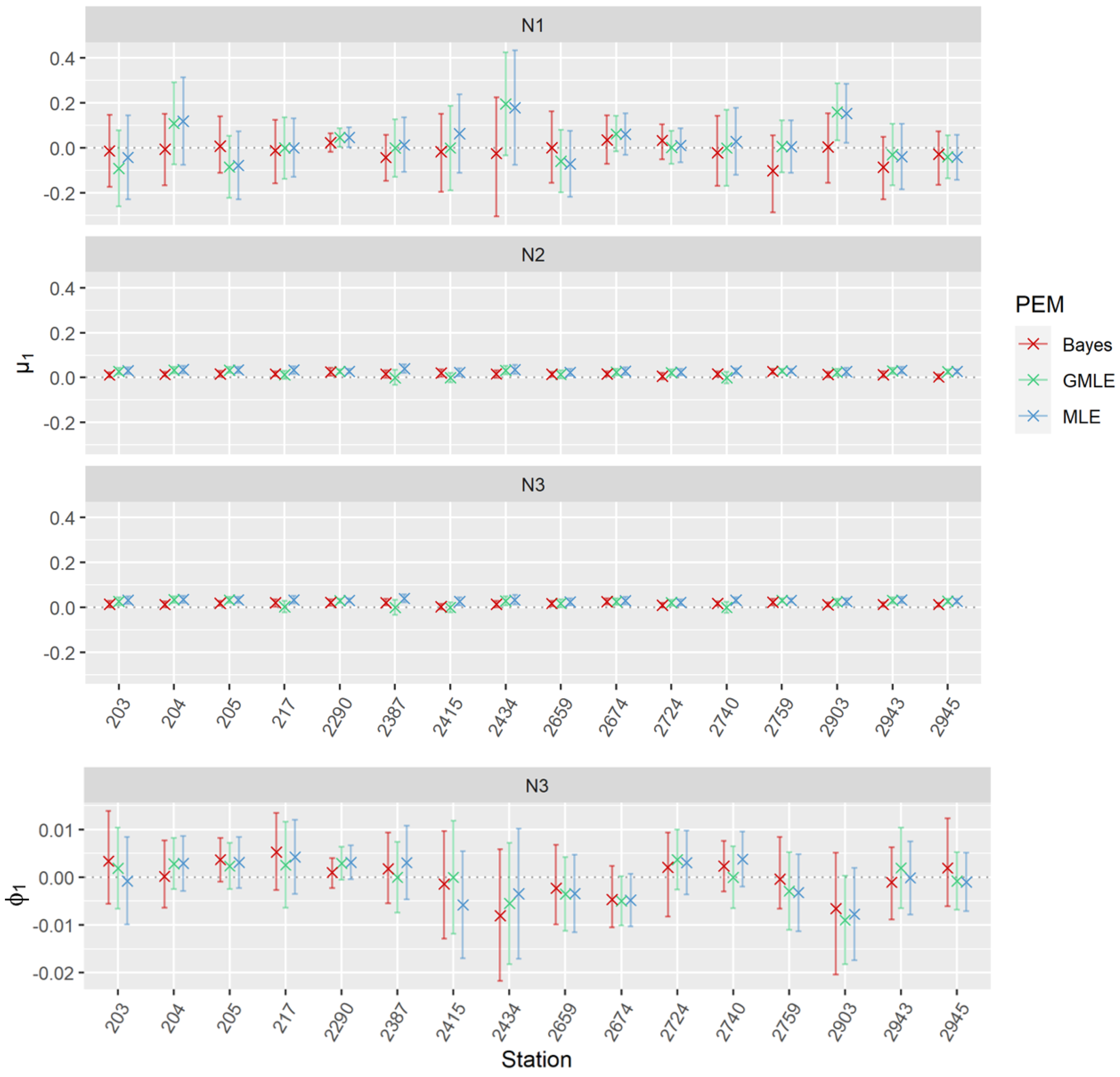
3.2. Justification and Evaluation of Non-Stationary EVA

In a preliminary step, trend analyses were performed to check whether or not non-stationary models can be applied. In approximately two thirds of the stations, a positive trend in the AMAX precipitation series over time was detected, indicating that time as a covariate (i.e., non-stationary model N1) can be applied.

For annual precipitation as a covariate, statistically significant correlation coefficients between annual precipitation and AMAX ranging between 0.36 and 0.55 were found. Trend tests were investigated for annual precipitation (i.e., the non-stationary models N2 and N3), but instead of indicating AMAX over time, it was now sorted by annual precipitation to enable the examination of trends in AMAX jointly with increasing annual precipitation. Results showed an increasing trend in AMAX with annual precipitation for all stations.

Figure 7 shows the slope in the location parameter of the non-stationary models (${\mu }_1$) which should reflect the above-mentioned dependencies of the covariate. For non-stationary model N1, estimates of ${\mu }_1$ were significantly positive for stations 2290 and 2903 for MLE and GMLE. At station 2290, this was due to low uncertainties, and at station 2903, the estimate of ${\mu }_1$ was exceptionally large so that even the lower CI was still positive. However, with the Bayesian estimation method, no estimation of ${\mu }_1$ was significantly different from zero. In contrast, for models N2 and N3, nearly all cases of ${\mu }_1$ were consistent in their sign and estimates were more consistent between different parameter estimation methods.

The slopes of the scale parameters ${\sigma }_1$ of non-stationary model N3 were not significantly different from zero for any station (Figure 7). However, for stations 2290 and 2674, the estimates for MLE and GMLE were still the most distinct, with a positive and negative slope, respectively. The uncertainties and variations in ${\mu }_1$ were by far the largest for non-stationary model N1. Differences between Bayesian estimates and the remaining two estimates (i.e., MLE and GMLE) were particularly large.

Furthermore, for the non-stationary model N1, goodness of fit according to AIC/DIC revealed hardly any improvements in model fit compared to stationary model S1. Exceptions were stations 2290 and 2903 with slightly decreased values of AIC and DIC. The likelihood ratio test also rejected the null hypothesis of no improvement with p-values of 0.038 and 0.034 for stations 2290 and 2903, respectively. The inclusion of annual precipitation into the location parameter (i.e., non-stationary model N2) for all stations increased the model fit according to both AIC/DIC and the likelihood ratio test. There was a tendency that stations with a higher correlation between annual precipitation and AMAX also increased the model fit.

For non-stationary model N3, model fit was again improved for all stations and all PEMs according to AIC, DIC, and lr tests.

3.3. Changes in Design Life Levels

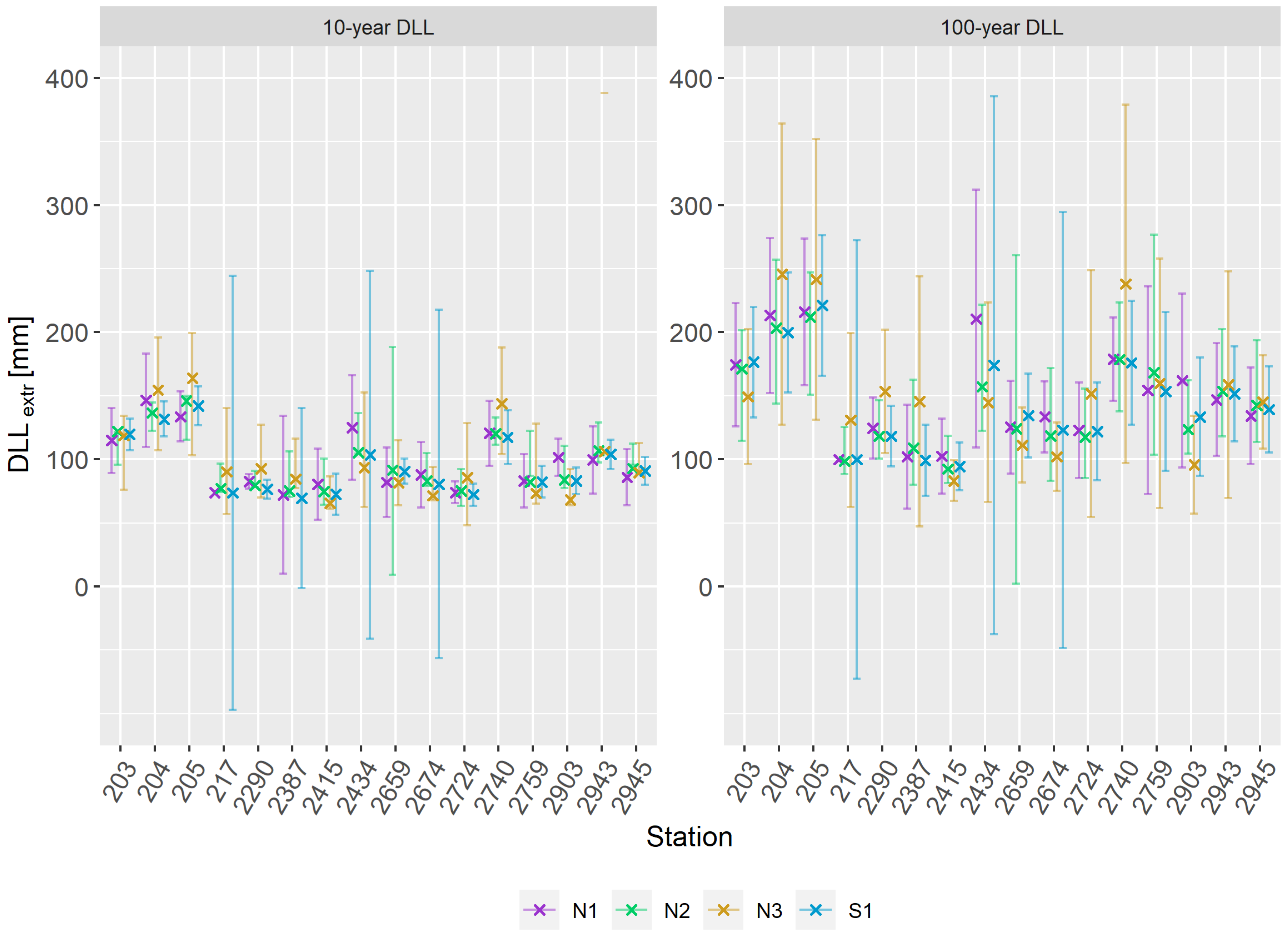
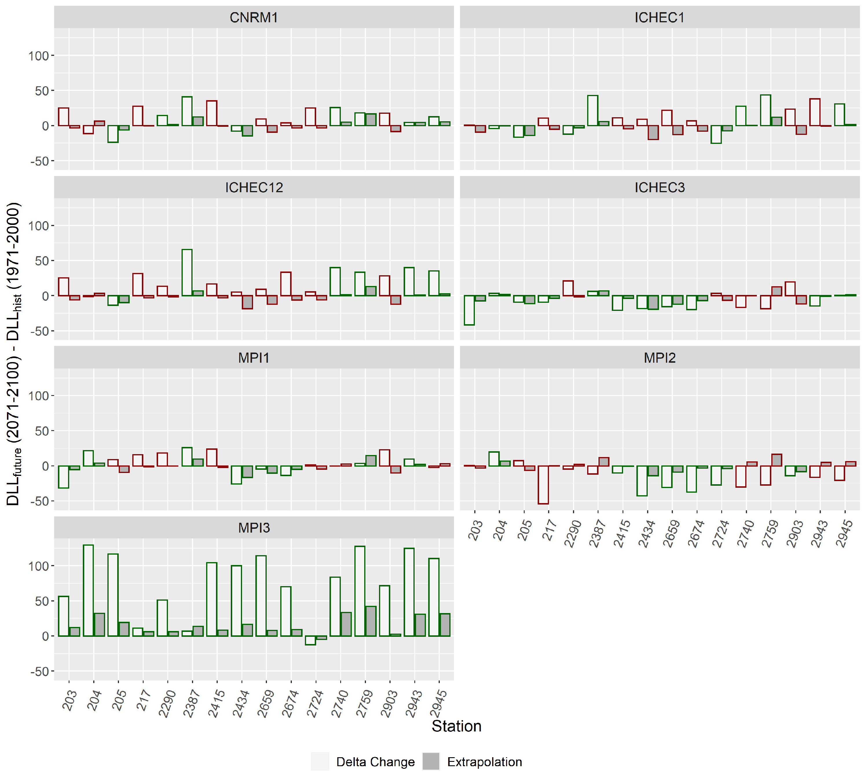
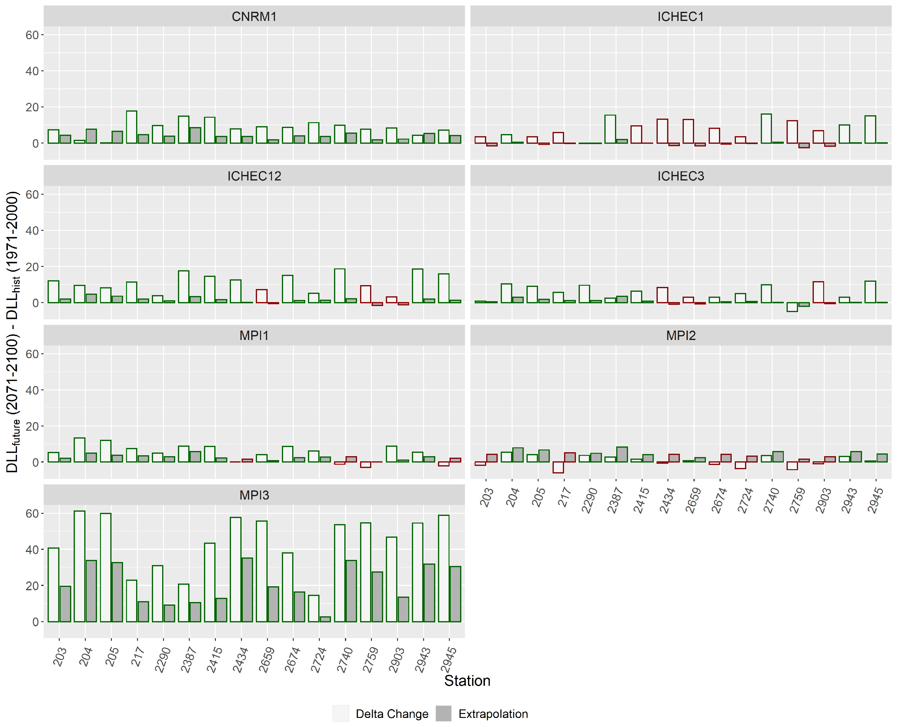
3.3.1. Extrapolation of Non-Stationary Models

Per definition, stationary DLLs equal the corresponding stationary RLs. Minor discrepancies are possible due to numerical difficulties. Differences between stationary and non-stationary DLLs were in general small for the historical time period (1971–2000) and only increased slightly with the extrapolation of non-stationary models for the future time period. Figure 8 shows 10-year and 100-year DLL_extr (2071–2100) values exemplary for the MLE method. The highest deviation from stationary DLLs/RLs is often achieved with model N3, which shows differences of up to 50 mm. One would expect increases with non-stationary models due to the above-described behavior of extreme precipitation. For the 100-year level, there is no clear pattern, as extrapolated non-stationary DLLs are sometimes even lower than stationary DLLs. Interestingly, for the 10-year level, almost all stations show slight increases in DLLs with the incorporation of non-stationarity. However, the differences are too small to derive robust conclusions. This aspect will be the subject of further research. It should be mentioned that lower uncertainty boundaries computed with the delta method again sometimes reach negative ranges, which is physically not consistent.

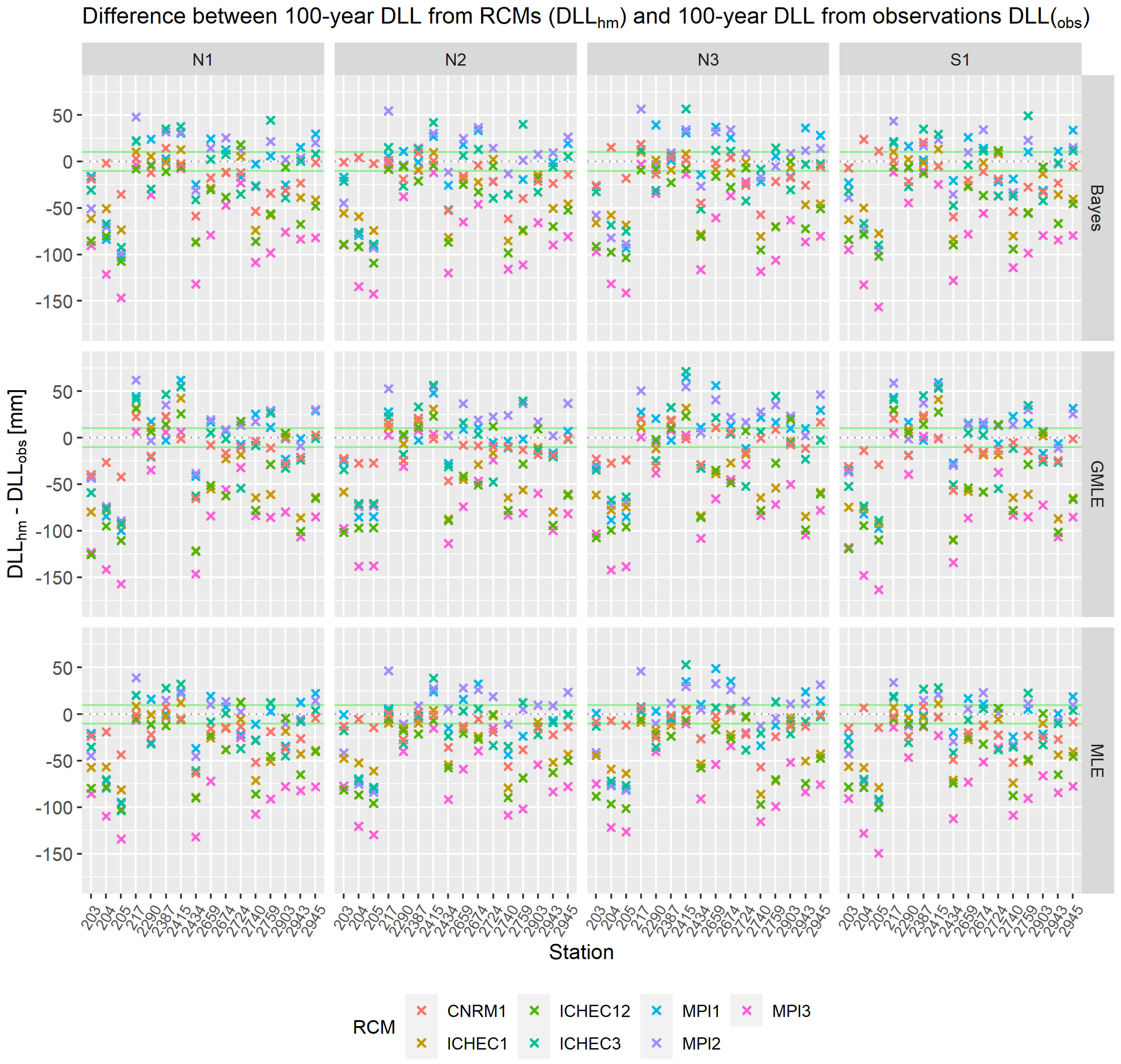
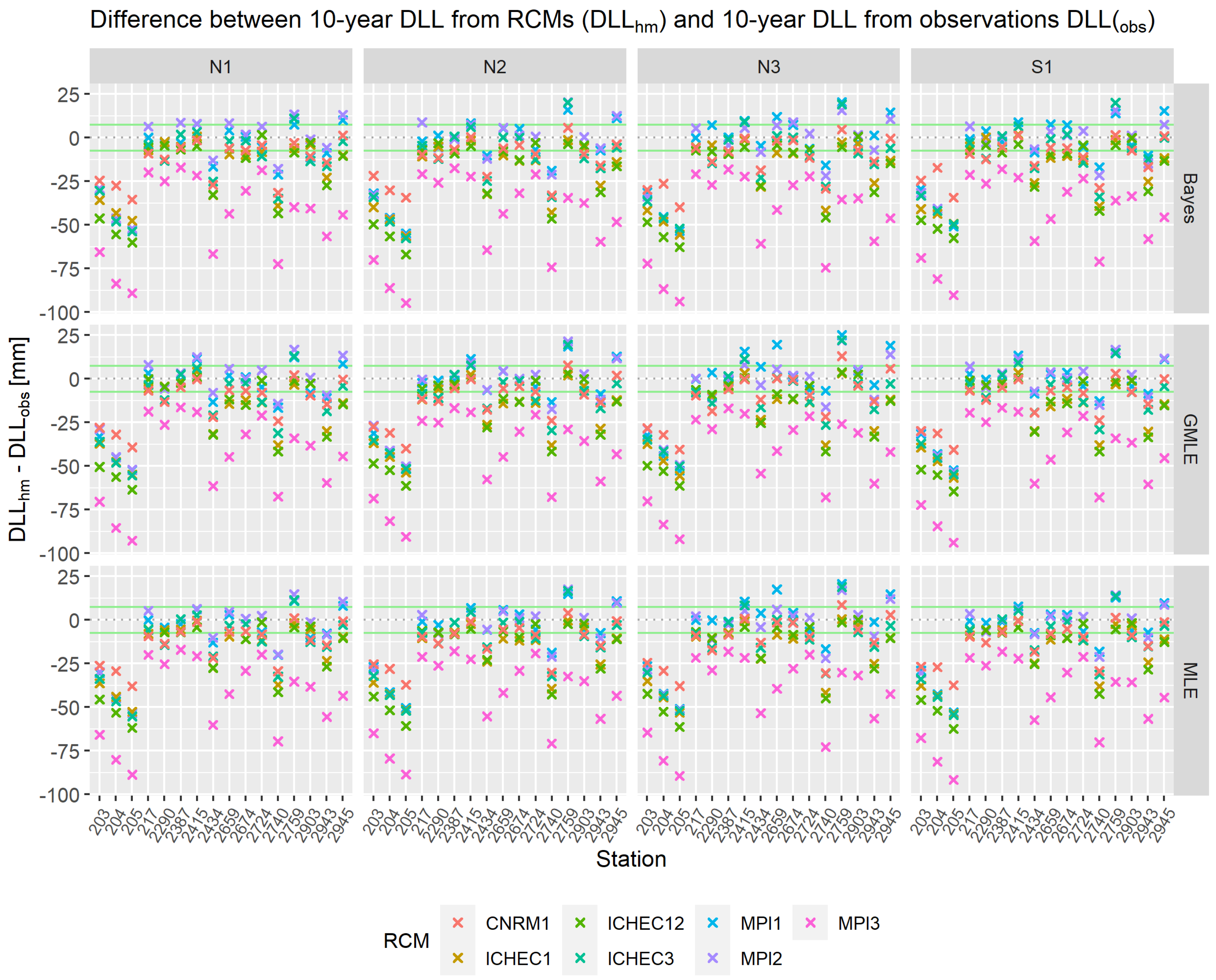
3.3.2. Non-Stationary EVA Using Regional Climate Model Output

As a second possibility to achieve future design life levels, climate models were considered. Firstly, the validation of RCM simulations showed a generally decent model fit, but RCMs did not fit well for specific stations.

All the RCMs underestimated AMAX from station data (stations 203, 204, 205, and 2740). The observational distribution showed both a higher median and a larger interquartile range (IRQ) in the data. Furthermore, MPI3 strongly underestimated the median and also in many cases the IRQ of the AMAX distribution for all stations. For a better insight into discrepancies, DLLs from historical model simulations DLL_hm were compared to DLLs from station data DLL_obs.

Figure 9 and Figure 10 show the differences between results from models and observations. The green marked area represents acceptable deviations which are approximately 10% of DLL_obs. The examined underestimation of AMAX from observations for stations 203, 204, 205, 2434, and 2740 for all RCMs was again visible with the DLLs of the simulations being much lower than the DLLs of the observations. In addition, it was found that MPI3 strongly underestimated the DLLs of observations with differences of up to 150 m which was approximately 75% of DLL_obs. These findings were even more pronounced for the GMLE and for the 10-year DLLs in Figure 10, where differences between DLL_hm and DLL_obs were substantially below the lower 10% line and MPI3 was, for all stations the model, with the strongest underestimation. According to mean absolute deviation between DLL_hm and DLL_obs, the best model was CNRM1 (∼19 mm for 100-year level/∼13 mm for 10-year level) followed by MPI1 (∼28 mm/∼14 mm) and MPI2 (∼30 mm/∼14 mm).

In the following, DLL_delta (2071–2100) are examined in greater detail and compared to DLL_extr (2071–2100). Since with seven different climate models the number of combinations increases drastically, now the focus lies on the MLE method as one of the standards and on the non-stationary model N2, which was selected as the best fitting model.

Figure 11 and Figure 12 show the projected changes in DLLs between 1971 and 2000 and 2071 and 2100 for the delta change method (RCMs) and the Extrapolation of non-stationary model N2. The colors of the bars indicate whether both methods coincide with the sign of change. Results from MPI3 are not considered reliable but are shown for the sake of completeness.

As described earlier for DLL_extr, at the 100-year level, there was no clear agreement on increases or decreases in DLLs. Similar to that, with the delta change method, again, no distinct tendency could be derived. For the 10-year level, however, RCMs predicted, for all stations, mainly increases in DLLs.

Hence, both methods of deriving future DLLs agree very well on the sign of change for the 10-year level, but at the 100-year level, changes in DLLs seem rather random, which is probably due to the predominance of uncertainties. Nevertheless, at both extreme levels, a tendency is visible that with CNRM1 and ICHEC12, increases are stronger, whereas with ICHEC3 and MPI2, the smallest increases or the largest decreases were computed. However, even when there was agreement on the sign of change, the actual size of increases or decreases in DLLs could strongly differ between the RCMs and the different methods. Changes were generally of higher values with the delta change method.

With the extrapolation of statistical models, only a shift in the distribution function of the existing dataset is performed, which does not result in strong changes if the covariate does not change remarkably over time. Hence, for the delta change method, the actual size of increases or decreases in DLLs can differ stronger between the seven RCMs.

In summary, for the 10-year level, increases of up to 20 mm can be expected, whereas for the 100-year level, projections lie within a range of +/−50 mm depending on the stations and RCMs.

4. Discussion

In this study, a variety of issues regarding extreme value analysis was investigated. Several approaches for traditional EVA were compared (i.e., the GEV and GP theoretical distribution functions as well as four different parameter estimation methods) while in the next step, non-stationary EVA was conducted in three different settings to account for changing statistical properties over time series. Additionally, it was tested whether simple RCM simulations (not bias-corrected) are appropriate as a supplement for station data and whether changes occur in DLLs by comparing the future period (2071–2100) with the historical period (1971–2000).

Due to the location of the study area and a data basis consisting of stations with different measuring sequences, it was partially possible to examine the performance with regard to the orography and the length of the time series.

As a first aspect, the effects of different methodologies in stationary EVA were discussed. Besides the common uncertainties regarding EVA due to lacking representativeness of the time series and presumed extrapolations into the future, results showed that different methods may introduce additional uncertainties.

Part of the differences in RLs between parameter estimation methods can be traced back to uncertain estimations of the scale and mainly the shape parameter. Since the shape parameter controls the tail behavior of the distributions and is generally quoted to be the most difficult to estimate [12,28], deviations can naturally become rather large when slight changes in the estimation procedure occur. However, as differences in the parameter estimates were large for all stations and some had a good agreement in RLs between different PEMs, deviations in the shape parameter alone were not the most crucial factor. The combination of scale and shape that alters the extreme characteristics of the distribution was considered the most crucial.

Although parameter estimates are the same between the 100-year and 10-year levels, deviations due to different PEMs were less pronounced at the 10-year level. This is because, for a 10-year RL, the database was about three times of the RP (in contrast to the 100-year level with a database of one to two-thirds of the RP); the 0.9 quantile is located at a more supported part of the distribution function and the impact of the tail behavior (and hence the parameter scale and shape) on RLs is much smaller. Therefore, to reduce the methodological uncertainties and to obtain more consistent results of return levels, sufficiently long time series would be necessary (which are often not available).

A detailed examination of the parameter estimation methods showed some peculiarities, especially for the Bayesian estimation method and GMLE; they are briefly discussed hereafter. Firstly, if the shape parameter of the GMLE method was smaller than zero, parameter estimates equaled those of L-moments, and thus the RLs were identical to those obtained by L-moments. Secondly, GMLE was introduced to improve estimates from MLE by restricting the estimates of the shape parameter to a likely range, but the incorporated prior distribution was based on flood analysis [20] so that the question arises whether this constraint is also suitable for precipitation data.

The higher values obtained by the Bayesian estimation method were in line with those of previous studies, which resulted in slightly higher estimates with Bayesian estimation than, for example, with MLE [29]. Nevertheless, in this study, for some stations, substantially large outliers in RLs were obtained with the Bayesian estimation method, which was not mentioned in Šraj et al. [29]. This was very pronounced at the 100-year level (Figure 3), but also at the 10-year level (Figure 4) for stations with short time series (i.e., time series length < 50 years) to a lower degree. The results of the Bayesian estimation method were not reproducible with different runs of the algorithm since the MCMC process contains some random components. Especially at stations with time series shorter than 50 years, the random part of the MCMC process resulted in more divergent design life levels. Thus, based on the findings of this study, results estimated with the Bayesian estimation method should be interpreted with great care when the underlying time series are relatively short (in this case, shorter than 50 years). However, the Bayesian estimation method, in general, provides more flexibility for improvement. For example, as an alternative to the here-used univariate normal distribution as a prior distribution, Coles and Powell [61] used a multivariate normal distribution based on estimates from other spatial locations to construct a prior, which probably had a higher potential to incorporate additional information to the estimation method. Therefore, a more thorough investigation to better quantify the various influences on the estimation technique could help to assess its reliability.

According to the literature, MLE has its peculiarities, too. For instance, the L-moments method is known to be more efficient than MLE, especially when the sample size is small (GP: < 500, GEV: < 50) [17,20,52,54], but these statements could not be confirmed in this study as RLs from MLE and L-moments were very similar, and no curious results were obtained using MLE at small sample sizes.

As already mentioned, another effect that arose due to time series length or rather the ratio between time series length and RP was the more consistent results between different parameter estimation methods for the 10-year level compared to the 100-year level. The 100-year RLs were therefore more sensitive to the selected methods of EVA and their slight discrepancies in the estimated parameters. In general, due to the nature of the function between RLs and RPs, the higher the RPs, the more uncertain the RLs [12,29]. A spatial pattern and distinct future changes in DLLs are therefore hardly visible at the 100-year level.

Furthermore, despite methodological uncertainties, scale, and especially shape parameters are highly sensitive to slight changes in the database. Since observations of extreme events are scarce, the presence or absence of individual extreme events in the investigated time series can have a strong impact on the estimated distribution function. In combination with the high spatiotemporal variability of heavy precipitation, computed design life levels of two neighboring stations can differ strongly, even if their statistical extreme behavior is actually the same [62,63]. This aspect hampered the comparison of DLLs from the observations and RCMs and presumably amplified the partly deficient accordance in this study. However, in fact, since for some stations—and mainly the climate results from MPI3—the distributions of AMAX were already dissimilar, differences in design life levels were probably because of lacking the representativeness of the RCMs for the study area. One possible reason is the different nature of both data sources, point measurements for the observations as well as areal estimates for the RCMs [64].

In this case, so-called Areal Reduction Factors (ARF) are suggested (e.g., [64]), or a distribution-scaling bias correction, or an approach particularly focusing on extreme values (e.g., [65]), which could possibly lead to more realistic results. The applied delta change method does not correct the precipitation distribution itself. Moreover, climate simulations with a higher spatial resolution (e.g., based on convection-permitting settings) are expected to better resemble the observed precipitation patterns [66].

In order to extrapolate the linear trend of non-stationary models with the help of RCM projections (i.e., annual precipitation) adequately, a sufficient fit between station data and RCMs is necessary. To fulfill this requirement, future projections of annual precipitation were bias-corrected via a linear transformation of the mean and standard deviation. With this method, an increase in the representativeness of the modeled annual precipitation was achieved. However, this method is too simple to adequately correct the extreme events.

For the non-stationary EVA, according to various goodness-of-fit criteria, the inclusion of annual precipitation into the location parameter (non-stationary models N2 and N3) improved the model fit. According to preliminary correlation coefficients and trend investigations, there was indeed a connection between annual precipitation and the time series of annual maxima. On the contrary, with non-stationary model N1, only stations with a trend in the time series of extremes (i.e., station 2290) indicated an improvement. Station 2290 clearly showed that sufficiently long time series are necessary to identify a temporal trend. The time series was about 60 years longer than at the other stations, and a significant time trend in the location parameter as well as a reasonably distinct trend in the scale parameter were obtained. This underpins the need for a sufficiently long time series for the non-stationary EVA. With model N3, the changes in the extrapolated DLLs were the largest since the trend in the scale parameter can strongly amplify the effect of the inherently incorporated trend in the location parameter. However, the inclusion of a time trend into the scale parameter (non-stationary model N3) considerably increased the confidence intervals (visible for the Bayesian estimation method in Figure 8) and, in addition, no trend in the scale parameter was found to be significant. Therefore, it is questionable whether a trend in the scale parameter provides credible information, and the results of this study emphasize the advice from previous studies (e.g., [22,35,41]), according to which a reasonable assumption of non-stationarity is crucial to achieving significant results and an increase in model fit. Furthermore, differences in design life levels between stationary and non-stationary models (i.e., S1, N1, N2, N3) were smaller for most stations than discrepancies due to different methodologies (i.e., assumptions of the underlying theoretical distributions and fitting procedures). The effect of the incorporation of non-stationarity into EVA, thus, lies within the range of uncertainties regarding EVA and makes its usage debatable.

However, it should be mentioned that other approaches to model extreme behavior and incorporate non-stationarity exist, so the representation in this study provides only a limited picture of potential methodological uncertainties.

The investigations of changes in DLLs between the historical time period of 1971–2000 and a future time period of 2071–2100 were based on results with MLE as well as model N2 as it would exceed the scope of this study to examine all cases. Usually, studies of changes in heavy and extreme precipitation reveal stronger increases or smaller decreases the higher the considered percentile [67]. Therefore, the question arises whether cases in which changes in 100-year design life levels were smaller than those in 10-year design life levels are reasonable or whether for the 100-year levels the aforementioned uncertainties dominated the estimation of design life levels. In general, it was difficult to examine changes in design life levels since statistical estimation is very uncertain and hence changes were too small to be significant.

Furthermore, it should be kept in mind that concomitant with the usage of RCMs, additional uncertainties about the future were introduced. Those are mainly the uncertainties due to unknown external boundary conditions and the lack of a complete understanding of the climate system. Regarding the former, in this study, the RCP8.5 was chosen, which resembles only one possible pathway of a high-impact radiative forcing and greenhouse gas concentration [6]. Other emission scenarios would possibly lead to different changes in DLLs. The limitation of climate models is also an important point since precipitation is still one of the variables with the highest uncertainties in climate models [68]. Especially individual storms and locally high rainfall events which are crucial for EVA are a well-known source of model errors [69].

Hence, due to the uncertainties regarding climate projections and EVA itself, changes in DLLs obtained with RCMs are to be treated with caution. However, due to a lack of observation data, climate simulations are often the only viable option to derive DLLs. This is particularly the case for sub-daily precipitation durations [64].

5. Conclusions

Since it is likely that climate change is altering the statistical characteristics of meteorological extremes in several regions worldwide, it is of great interest to adapt to changing conditions in the best possible way. This study investigated several options for the derivation of daily precipitation extremes for a study area in an alpine region in Southern Germany. The obtained results underpin the large uncertainties associated with the stationary and non-stationary EVA approaches. Since different approaches in stationary EVA showed partially strong discrepancies in the derived DLLs, the potential benefits of non-stationary EVA vanish in those methodological uncertainties. The following conclusions are drawn from this study:

• For the end of this century in the Oberland region, there is no robust tendency towards increased precipitation extremes expressed as DLLs, even under the assumption of the high-impact RCP8.5 emission scenario. This is confirmed following approaches based on extrapolated observation data and RCM output.
• It is further concluded that, in practice, non-stationary EVA is not necessarily needed. Non-stationary EVA potentially offers an added value in cases when long series of observations (in the order of 100 years) are available and robust trends of extremes can be derived.
• As observation data are often not sufficient in practice, RCM data driven by Reanalysis data provide an alternative for filling data gaps in space and time.
• RCMs also provide potential options for non-stationary EVA under future climate conditions; however, additional uncertainties such as the unknown future emissions as well as uncertainties from different large-scale forcing (i.e., different GCMs) and RCM parameterizations must be considered.
• Despite all of the methodological uncertainties, EVA currently provides a sound solution to derive hydrometeorological design values for infrastructure that has to withstand extreme events.

Based on the findings of this study, it is suggested to apply different extreme value models (stationary as well as non-stationary) based on different theoretical distribution functions and parameter estimation methods. This allows one accounting for the methodological inherent uncertainties of the DLLs for the future. Moreover, the impact of different bias correction methods should be considered in this context. More research on more sophisticated bias correction approaches (as applied in this study) is needed, which either correct the whole distribution of precipitation or focus on the (extreme) tails of the distribution.

References

- Swiss Re. Natural Catastrophes in 2021: The Floodgates Are Open; Technical Report; Swiss Re Institute: Zürich, Switzerland, 2022. [Google Scholar]
- Junghänel, T.; Bissolli, P.; Daßler, J.; Fleckenstein, R.; Imbery, F.; Janssen, W.; Kaspar, F.; Lengfeld, K.; Leppelt, T.; Rauthe, M.; et al. Hydro-Klimatologische Einordnung der Stark-und Dauerniederschläge in Teilen Deutschlands im Zusammenhang mit dem Tiefdruckgebiet “Bernd” vom 12. bis 19. Juli 2021; Technical Report; Deutscher Wetterdienst: Offenbach am Main, Germany, 2021. [Google Scholar]
- Lehmkuhl, F.; Schüttrumpf, H.; Schwarzbauer, J.; Brüll, C.; Dietze, M.; Letmathe, P.; Völker, C.; Hollert, H. Assessment of the 2021 summer flood in Central Europe. Environ. Sci. Eur. 2022, 34, 107. [Google Scholar] [CrossRef]
- Masson-Delmotte, V.; Zhai, P.; Pirani, A.; Connors, S.L.; Péan, C.; Yang, C.; Leah, G.; Gomis, M.I.; Matthews, J.B.R.; Berger, S.; et al. Summary for Policymakers. In Climate Change 2021: The Physical Science Basis; Contribution of Working Group I to the Sixth Assessment Report of the Intergovernmental Panel on Climate Change; Cambridge University Press: Cambridge, UK; New York, NY, USA, 2021; pp. 3–32. [Google Scholar] [CrossRef]
- Pörtner, H.-O.; Roberts, D.C.; Tignor, M.M.B.; Poloczanska, E.; Mintenbeck, K.; Alegría, A.; Craig, M.; Langsdorf, S.; Löschke, S.; Möller, V.; et al. (Eds.) Climate Change 2022: Impacts, Adaptation and Vulnerability; Working Group II Contribution to the IPCC Sixth Assessment Report; Cambridge University Press: Cambridge, UK; New York, NY, USA, 2022. [Google Scholar]
- van Vuuren, D.P.; Edmonds, J.; Kainuma, M.; Riahi, K.; Thomson, A.; Hibbard, K.; Hurtt, G.C.; Kram, T.; Krey, V.; Lamarque, J.F.; et al. The representative concentration pathways: An overview. Clim. Chang. 2011, 109, 5–31. [Google Scholar] [CrossRef]
- Madakumbura, G.D.; Thackeray, C.W.; Norris, J.; Goldenson, N.; Hall, A. Anthropogenic influence on extreme precipitation over global land areas seen in multiple observational datasets. Nat. Commun. 2021, 12, 3944. [Google Scholar] [CrossRef] [PubMed]
- Martinkova, M.; Kysely, J. Overview of observed clausius-clapeyron scaling of extreme precipitation in midlatitudes. Atmosphere 2020, 11, 786. [Google Scholar] [CrossRef]
- Dingman, S.L. Physical Hydrology; Waveland Press, Inc.: Long Grove, IL, USA, 2015. [Google Scholar]
- Salas, J.D.; Obeysekera, J.; Vogel, R.M. Techniques for assessing water infrastructure for nonstationary extreme events: A review. Hydrol. Sci. J. 2018, 63, 325–352. [Google Scholar] [CrossRef]
- Slater, L.J.; Anderson, B.; Buechel, M.; Dadson, S.; Han, S.; Harrigan, S.; Kelder, T.; Kowal, K.; Lees, T.; Matthews, T.; et al. Nonstationary Weather and Water Extremes: A Review of Methods for Their Detection, Attribution, and Management. Hydrol. Earth Syst. Sci. 2021, 25, 3897–3935. [Google Scholar] [CrossRef]
- Coles, S. An Introduction to Statistical Modeling of Extreme Values; Springer Series in Statistics; Springer: Berlin/Heidelberg, Germany, 2001. [Google Scholar]
- Stephenson, A.; Tawn, J. Bayesian Inference for Extremes: Accounting for the Three Extremal Types; Springer Science + Business Media, Inc.: Dordrecht, The Netherlands, 2004; pp. 291–307. [Google Scholar]
- Wi, S.; Valdés, J.B.; Steinschneider, S.; Kim, T.W. Non-stationary frequency analysis of extreme precipitation in South Korea using peaks-over-threshold and annual maxima. Stoch. Environ. Res. Risk Assess. 2016, 30, 583–606. [Google Scholar] [CrossRef]
- Scarrott, C.; Macdonald, A. A Review of Extreme Value Threshold Estimation And Uncertainty Quantification. REVSTAT Stat. J. 2012, 10, 33–60. [Google Scholar]
- Beirlant, J.; Goegebeur, Y.; Teugels, J.; Segers, J.; De Waal, D.; Ferro, C. Statistics of Extremes: Theory and Applications; John Wiley & Sons Ltd.: Chichester, UK, 2004. [Google Scholar]
- Martins, E.S.; Stedinger, J.R. Generalized maximum likelihood Pareto-Poisson estimators for partial duration series. Water Resour. Res. 2001, 37, 2551–2557. [Google Scholar] [CrossRef]
- Jenkinson, A.F. The frequency distribution of the annual maximum (or minimum) values of meteorological elements. Q. J. R. Meteorol. Soc. 1955, 81, 158–171. [Google Scholar] [CrossRef]
- Cheng, L.; AghaKouchak, A.; Gilleland, E.; Katz, R.W. Non-stationary extreme value analysis in a changing climate. Clim. Chang. 2014, 127, 353–369. [Google Scholar] [CrossRef]
- Martins, E.S.; Stedinger, J.R. Generalized maximum-likelihood generalized extreme-value quantile estimators for hydrologic data. Water Resour. Res. 2000, 36, 737–744. [Google Scholar] [CrossRef]
- Reis, D.S.; Stedinger, J.R. Bayesian MCMC flood frequency analysis with historical information. J. Hydrol. 2005, 313, 97–116. [Google Scholar] [CrossRef]
- Serinaldi, F.; Kilsby, C.G. Stationarity is undead: Uncertainty dominates the distribution of extremes. Adv. Water Resour. 2015, 77, 17–36. [Google Scholar] [CrossRef]
- Villarini, G.; Smith, J.A.; Serinaldi, F.; Bales, J.; Bates, P.D.; Krajewski, W.F. Flood frequency analysis for nonstationary annual peak records in an urban drainage basin. Adv. Water Resour. 2009, 32, 1255–1266. [Google Scholar] [CrossRef]
- Mehmood, A.; Jia, S.; Mahmood, R.; Yan, J.; Ahsan, M. Non-Stationary Bayesian Modeling of Annual Maximum Floods in a Changing Environment and Implications for Flood Management in the Kabul River Basin, Pakistan. Water 2019, 11, 1246. [Google Scholar] [CrossRef]
- Feldmann, D.; Laux, P.; Heckl, A.; Schindler, M.; Kunstmann, H. Near surface roughness estimation: A parameterization derived from artificial rainfall experiments and two-dimensional hydrodynamic modelling for multiple vegetation coverages. J. Hydrol. 2023, 617, 128786. [Google Scholar] [CrossRef]
- Villarini, G.; Taylor, S.; Wobus, C.; Vogel, R.; Hecht, J.; White, K.; Baker, B.; Gilroy, K.; Olsen, J.R.; Raff, D. Floods and Nonstationarity: A Review; Technical Report, CWTS 2018-01; U.S. Army Corps of Engineers: Washington, DC, USA, 2018. [Google Scholar]
- Rootzén, H.; Katz, R.W. Design Life Level: Quantifying risk in a changing climate. Water Resour. Res. 2013, 49, 5964–5972. [Google Scholar] [CrossRef]
- Cooley, D. Return Periods and Return Levels Under Climate Change. In Extremes in a Changing Climate: Detection, Analysis and Uncertainty; AghaKouchak, A., Easterling, D., Hsu, K., Schubert, S., Sorooshian, S., Eds.; Springer: Dordrecht, The Netherlands, 2013; pp. 97–114. [Google Scholar] [CrossRef]
- Šraj, M.; Viglione, A.; Parajka, J.; Blöschl, G. The influence of non-stationarity in extreme hydrological events on flood frequency estimation. J. Hydrol. Hydromech. 2016, 64, 426–437. [Google Scholar] [CrossRef]
- Katz, R.W. Statistical Methods for Nonstationary Extremes. In Extremes in a Changing Climate: Detection, Analysis and Uncertainty; AghaKouchak, A., Easterling, D., Hsu, K., Schubert, S., Sorooshian, S., Eds.; Springer: Dordrecht, The Netherlands, 2013; pp. 15–37. [Google Scholar] [CrossRef]
- Wunsch, C. The Interpretation of Short Climate Records, with Comments on the North Atlantic and Southern Oscillations. Bull. Am. Meteorol. Soc. 1999, 80, 245–256. [Google Scholar] [CrossRef]
- Koutsoyiannis, D. Climate change, the Hurst phenomenon, and hydrological statistics. Hydrol. Sci. J. 2003, 48, 3–24. [Google Scholar] [CrossRef]
- Matalas, N.C. Comment on the Announced Death of Stationarity. J. Water Resour. Plan. Manag. 2012, 138, 311–312. [Google Scholar] [CrossRef]
- Bayazit, M. Nonstationarity of Hydrological Records and Recent Trends in Trend Analysis: A State-of-the-art Review. Environ. Process. 2015, 2, 527–542. [Google Scholar] [CrossRef]
- Koutsoyiannis, D.; Montanari, A. Negligent killing of scientific concepts: The stationary case. Hydrol. Sci. J. 2015, 60, 1174–1183. [Google Scholar] [CrossRef]
- Salas, J.D.; Obeysekera, J. Revisiting the Concepts of Return Period and Risk for Nonstationary Hydrologic Extreme Events. J. Hydrol. Eng. 2014, 19, 554–568. [Google Scholar] [CrossRef]
- Hu, Y.; Liang, Z.; Singh, V.P.; Zhang, X.; Wang, J.; Li, B.; Wang, H. Concept of Equivalent Reliability for Estimating the Design Flood under Non-stationary Conditions. Water Resour. Manag. 2018, 32, 997–1011. [Google Scholar] [CrossRef]
- Emeis, S. Analysis of decadal precipitation changes at the northern edge of the alps. Meteorol. Z. 2021, 30, 285–293. [Google Scholar] [CrossRef]
- Nissen, K.M.; Ulbrich, U.; Leckebusch, G.C. Vb cyclones and associated rainfall extremes over central Europe under present day and climate change conditions. Meteorol. Z. 2013, 22, 649–660. [Google Scholar] [CrossRef]
- Peristeri, M.; Ulrich, W.; Smith, R.K. Genesis conditions for thunderstorm growth and the development of a squall line in the northern Alpine foreland. Meteorol. Atmos. Phys. 2000, 72, 251–260. [Google Scholar] [CrossRef]
- Koutsoyiannis, D. Nonstationarity versus scaling in hydrology. J. Hydrol. 2006, 324, 239–254. [Google Scholar] [CrossRef]
- Giorgi, F.; Jones, C.; Asrar, G.R. Addressing climate information needs at the regional level: The CORDEX framework. WMO Bull. 2009, 58, 239–254. [Google Scholar]
- Jacob, D.; Petersen, J.; Eggert, B.; Alias, A.; Christensen, O.B.; Bouwer, L.M.; Braun, A.; Colette, A.; Déqué, M.; Georgievski, G.; et al. EURO-CORDEX: New high-resolution climate change projections for European impact research. Reg. Environ. Chang. 2014, 14, 563–578. [Google Scholar] [CrossRef]
- Mascaro, G.; Viola, F.; Deidda, R. Evaluation of Precipitation From EURO-CORDEX Regional Climate Simulations in a Small-Scale Mediterranean Site. J. Geophys. Res. Atmos. 2018, 123, 1604–1625. [Google Scholar] [CrossRef]
- Giorgetta, M.A.; Jungclaus, J.; Reick, C.H.; Legutke, S.; Bader, J.; Böttinger, M.; Brovkin, V.; Crueger, T.; Esch, M.; Fieg, K.; et al. Climate and carbon cycle changes from 1850 to 2100 in MPI-ESM simulations for the Coupled Model Intercomparison Project phase 5. J. Adv. Model. Earth Syst. 2013, 5, 572–597. [Google Scholar] [CrossRef]
- Nolan, P.; Mckinstry, A. EC-Earth Global Climate Simulations-Ireland’s Contributions to CMIP6; Technical Report; Environmental Protection Agency: Wexford, Ireland, 2020. [Google Scholar]
- Laux, P.; Rötter, R.P.; Webber, H.; Dieng, D.; Rahimi, J.; Wei, J.; Faye, B.; Srivastana, A.; Bliefernicht, J.; Adeyeri, O.; et al. To bias correct or not to bias correct? An agricultural impact modelers’ perspective on regional climate model data. Agric. For. Meteorol. 2021, 304–305, 108406. [Google Scholar] [CrossRef]
- Pickands, J. Statistical Inference Using Extreme Order Statistics. Source Ann. Stat. 1975, 3, 119–131. [Google Scholar]
- Gilleland, E.; Katz, R.W. ExtRemes 2.0: An extreme value analysis package in R. J. Stat. Softw. 2016, 72, 1–39. [Google Scholar] [CrossRef]
- Anagnostopoulou, C.; Tolika, K. Extreme precipitation in Europe: Statistical threshold selection based on climatological criteria. Theor. Appl. Climatol. 2012, 107, 479–489. [Google Scholar] [CrossRef]
- Katz, R.W.; Parlange, M.B.; Naveau, P. Statistics of extremes in hydrology. Adv. Water Resour. 2002, 25, 1287–1304. [Google Scholar] [CrossRef]
- Coles, S.G.; Dixon, M.J. Likelihood-Based Inference for Extreme Value Models. Extremes 1999, 2, 5–23. [Google Scholar] [CrossRef]
- Hosking, J.R.M. L-Moments: Analysis and Estimation of Distributions using Linear Combinations of Order Statistics. Source J. R. Stat. Soc. Ser. Methodol. 1990, 52, 105–124. [Google Scholar] [CrossRef]
- Hosking, J.R.M.; Wallis, J.R. Parameter and Quantile Estimation for the Generalized Pareto Distribution. Technometrics 1987, 29, 339–349. [Google Scholar] [CrossRef]
- Cavanaugh, J.E.; Neath, A.A. The Akaike information criterion: Background, derivation, properties, application, interpretation, and refinements. Wiley Interdiscip. Rev. Comput. Stat. 2019, 11, e1460. [Google Scholar] [CrossRef]
- Hawkins, E.; Osborne, T.M.; Ho, C.K.; Challinor, A.J. Calibration and bias correction of climate projections for crop modelling: An idealised case study over Europe. Agric. For. Meteorol. 2013, 170, 19–31. [Google Scholar] [CrossRef]
- Navarro-Racines, C.; Tarapues, J.; Thornton, P.; Jarvis, A.; Ramirez-Villegas, J. High-resolution and bias-corrected CMIP5 projections for climate change impact assessments. Sci. Data 2020, 7, 7. [Google Scholar] [CrossRef] [PubMed]
- Dang, Q.; Laux, P.; Kunstmann, H. Future high- and low-flow estimations for Central Vietnam: A hydro-meteorological modelling chain approach. Hydrol. Sci. J. 2017, 62, 1867–1889. [Google Scholar] [CrossRef]
- Teutschbein, C.; Seibert, J. Bias correction of regional climate model simulations for hydrological climate-change impact studies: Review and evaluation of different methods. J. Hydrol. 2012, 456–457, 12–29. [Google Scholar] [CrossRef]
- Müller, C.; Voigt, M.; Iber, C.; Sauer, T. Starkniederschläge: Entwicklung in Vergangenheit und Zukunft; Technical Report; KLIWA: Offenbach, Germany, 2019. [Google Scholar]
- Coles, S.G.; Powell, E.A. Bayesian Methods in Extreme Value Modelling: A Review and New Developments. Int. Stat. Rev. 1996, 64, 119–136. [Google Scholar] [CrossRef]
- Lengfeld, K.; Kirstetter, P.E.; Fowler, H.J.; Yu, J.; Becker, A.; Flamig, Z.; Gourley, J. Use of radar data for characterizing extreme precipitation at fine scales and short durations. Environ. Res. Lett. 2020, 15, 085003. [Google Scholar] [CrossRef]
- Junghänel, T.; Ertel, H.; Deutschländer, T.; Wetterdienst, D.; Hydrometeorologie, A. Bericht zur Revision der Koordinierten Starkregenregionalisierung und-Auswertung des Deutschen Wetterdienstes in der Version 2010; Technical Report; Deutscher Wetterdienst Abteilung Hydrometeorologie: Offenbach am Main, Germany, 2017. [Google Scholar]
- Poschlod, B.; Ludwig, R.; Sillmann, J. Ten-year return levels of sub-daily extreme precipitation over Europe. Earth Syst. Sci. Data 2021, 13, 983–1003. [Google Scholar] [CrossRef]
- Maity, R.; Suman, M.; Laux, P.; Kunstmann, H. Bias correction of zero-inflated RCM precipitation fields: A copula-based scheme for both mean and extreme conditions. J. Hydrometeorol. 2019, 20, 595–611. [Google Scholar] [CrossRef]
- Warscher, M.; Wagner, S.; Marke, T.; Laux, P.; Smiatek, G.; Strasser, U.; Kunstmann, H. A 5 km resolution regional climate simulation for Central Europe: Performance in high mountain areas and seasonal, regional and elevation-dependent variations. Atmosphere 2019, 10, 682. [Google Scholar] [CrossRef]
- Ban, N.; Schmidli, J.; Schär, C. Heavy precipitation in a changing climate: Does short-term summer precipitation increase faster? Geophys. Res. Lett. 2015, 42, 1165–1172. [Google Scholar] [CrossRef]
- Kyselý, J.; Rulfová, Z.; Farda, A.; Hanel, M. Convective and stratiform precipitation characteristics in an ensemble of regional climate model simulations. Clim. Dyn. 2016, 46, 227–243. [Google Scholar] [CrossRef]
- Berthou, S.; Kendon, E.J.; Chan, S.C.; Ban, N.; Leutwyler, D.; Schär, C.; Fosser, G. Pan-European climate at convection-permitting scale: A model intercomparison study. Clim. Dyn. 2020, 55, 35–59. [Google Scholar] [CrossRef]