
Spatiotemporal Variation and Driving Factors for NO2 in Mid-Eastern China

1
School of Environment and Energy Engineering, Anhui Jianzhu University, Hefei 230601, China
2
Anhui Provincial Key Laboratory of Environmental Pollution Control and Resource Reuse, Hefei 230601, China
*
Author to whom correspondence should be addressed.
Atmosphere 2023, 14(9), 1369; https://doi.org/10.3390/atmos14091369
Submission received: 8 July 2023
/
Revised: 15 August 2023
/
Accepted: 28 August 2023
/
Published: 30 August 2023
(This article belongs to the Special Issue Air Quality and the Implementation of Sustainable Development Goals)
Abstract
:Nitrogen dioxide (NO2) is one of the major air pollutants in cities across mid-eastern China. Comprehending the spatial and temporal dynamics of NO2 drivers in various urban areas is imperative for tailoring effective air control strategies. Using data from ground-based monitoring stations, we investigated the impact of socioeconomic and meteorological factors on NO2 concentrations in cities in mid-eastern China from 2015 to 2021 using the Geographically and Temporally Weighted Regression (GTWR) model. The findings reveal a notable reduction of over 10% in NO2 concentrations since 2015 in most cities, notably a 50.5% decrease in Bozhou. However, certain areas within Anhui and Jiangsu have experienced an increase in NO2 concentrations. Significant spatial heterogeneity is observed in the relationship between NO2 concentrations and influencing factors. The permanent population density (POP) and the electricity consumption (EC) of the entire society exhibited the strongest correlations with NO2 concentrations, with average coefficients of 0.431 and 0.520, respectively. Furthermore, other economic factors such as urbanization rate (UR), the share of secondary sector output in total GDP (IS), and the coverage rate of urban green areas (CG) were predominantly positively correlated, while GDP per capita (PGDP) and civil car vehicles (CV) demonstrated primarily negative correlations. Furthermore, we examined the correlations between four meteorological factors (temperature, relative humidity, wind speed, and precipitation) and NO2 concentrations. All these factors exhibited negative correlations with NO2 concentrations. Among them, temperature exhibited the strongest negative correlation, with a coefficient of −0.411. This research may contribute valuable insights and guidance for developing air emission reduction policies in various cities in mid-eastern China.
1. Introduction
Recent years have witnessed rapid urbanization and industrialization in China, resulting in a significant rise in air pollution and growing concerns regarding climate issues [1]. NO2, as a major air pollutant, significantly impacts air quality, plays a significant role in the formation of acid rain and photochemical smog, and serves as a precursor to the formation of PM2.5 and O3 [2,3]. In addition, NO2 exposure can pose a risk to human health by stimulating the respiratory system [4], leading to diseases such as pneumonia and cancer [5] and triggering mental illness and childhood asthma [6,7]. Furthermore, elevated concentrations of NO2 can negatively impact vegetation growth and harm local ecosystems [8].
The spatial and temporal analysis of NO2 using satellite data from the Ozone Monitoring Instrument (OMI) of the National Aeronautics and Space Administration has been extensively studied [9]. By analyzing the changes in tropospheric NO2 vertical column density in East China from 2005 to 2020 to investigate the factors contributing to the reduction in tropospheric NO2 during the COVID-19 outbreak [10], Zheng et al. [11] analyzed the long-term distribution characteristics of NO2 concentrations in the Inner Mongolia urban cluster from 2005 to 2016 revealing an initial upward trend followed by a subsequent downward trend. However, OMI satellite data are often limited by poor resolution and a high number of missing values [12]. Moreover, it does not capture small-scale changes in concentrations [13]. Consequently, studies investigating spatial and temporal variability frequently rely on data obtained from ground-based monitoring sites. For example, recent research conducted by Hůnová et al. [14] documented a significant decrease in NO2 concentrations at various locations in the Czech Republic. Similarly, Shen et al. [15] observed an increase in the diurnal variation in NO2 concentrations in eastern China, which was attributed to changes in anthropogenic emissions.
Currently, it is a long-term strategic priority for China’s national development to actively promote pollution reduction. Therefore, investigating the relationship between changes in NO2 concentration and driving factors has emerged as a prominent research topic. NO2 concentrations typically vary due to three primary factors: emissions, meteorology, and atmospheric chemical processes [16,17]. High temperatures, precipitation, and higher wind speeds have been identified as beneficial factors in reducing NO2 concentrations [18,19]. Social factors, including industrial emissions, traffic emissions, energy consumption, industrial structure, and population density, have been recognized as essential influencers affecting NO2 concentrations [20,21,22]. Wang et al. [23] analyzed the factors driving vehicle NOx emissions from 2005 to 2015 and identified economic development and road vehicle carrying capacity as the primary drivers of emissions growth. Xu et al. [24] discovered that different levels of urbanization have varying effects on NOx emissions. Zhang et al. [25] examined NOx emissions and intensity changes in China and demonstrated that energy efficiency improvements and end-of-pipe emission reduction treatments were effective in reducing NOx emissions. They found that the main impediment to reducing NOx emissions and intensity was the final demand effect, with investment and consumption effects being the primary influences. These studies have characterized NOx emissions in urban environments from different perspectives and identified the main source contributions and potential drivers of NOx in urban environments. However, we also find that many of these studies have not provided more scientific explanations from the perspective of urban differences or have not paid enough attention to the relationship between urban development trajectories and economic structure as reflected in such differences due to the limited time and space sample size.
Several methods, including structural decomposition analysis [26], index decomposition analysis [27], logistic mean divided index [28], geographical detector model [29], and geographically weighted regression models (GWR) [30], have been employed to study the drivers of NO2 concentration changes. However, these methods only provide singular insights into NO2 concentration changes, focusing on a specific time or spatial context. The Geographically and Temporally Weighted Regression (GTWR) model extends the GWR model by constructing a matrix considering spatial and temporal distances. Consequently, it enables a comprehensive reflection of the spatial location characteristics of the model and the influence of temporal factors [31]. The GTWR model has been extensively employed in numerous studies to investigate the spatiotemporal heterogeneity between dependent and independent variables. These studies have examined the impact of population movement on the spread of COVID-19 [32] and identified the primary influences on soil Cd pollution in diverse regions [33], and the spatiotemporal variation in CO2 emissions resulting from the ‘coal-to-gas’ conversion in heating areas [34].
In this study, we investigate the trends and spatial characteristics of NO2 concentrations in central-eastern Chinese cities. The data used for analysis was collected from Chinese air quality monitoring stations between 2015 and 2021. Furthermore, we employ the GTWR model to analyze the spatial and temporal distribution characteristics of the factors influencing changes in NO2 concentrations. This work aims to understand the trends in nitrogen dioxide concentrations in different cities in the region in recent years and to identify the drivers behind these trends. This may be critical for population health and environmental protection and provide valuable policy insights and inspiration for the cities involved.
2. Materials and Methods
2.1. Study Areas
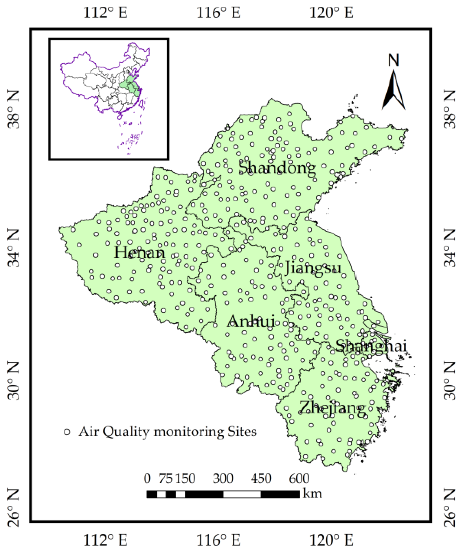
The study area encompasses six provincial administrative units in mid-eastern China: Shandong, Henan, Anhui, Jiangsu, Zhejiang, and Shanghai. The topography of each province is as follows: Anhui Province is characterized by plains, hills, and low mountains. The terrain generally exhibits a “high in the south and low in the north” pattern. Zhejiang Province is elevated in the southwest and descends toward the northeast, with mountains and hills being the dominant features. Shandong Province displays a diverse topography, including mountains, hills, and plains. Jiangsu Province is primarily flat and low-lying, mainly comprising plains, while some hilly terrain can be found in the southwest. Henan Province features a mountainous west and a flat east. Shanghai is situated on the front of the Yangtze River Delta Plain, with its terrain being predominantly flat. Figure 1 shows the geographic location of the study area and the distribution of air quality monitoring stations. According to the China Statistical Yearbook in 2022 (http://www.stats.gov.cn/sj/ndsj/2022/indexch.htm, accessed on 1 February 2023), the six provincial administrative units within the study area account for 36.89% of China’s GDP and 30.94% of the country’s total population. This region holds great significance in China because it includes the Yangtze River Delta urban agglomeration, which is one of the three largest urban agglomerations in the country. Consequently, the study area has experienced rapid development in recent years, causing advanced industrialization and a substantial influx of people. However, the area’s developed economy, dense population, and high level of industrialization have also contributed to its overall poor air quality.
2.2. Data Sources
2.2.1. NO2 Concentration Data
Hourly NO2 concentration data for 2015–2021 were obtained from the China General Environmental Monitoring Station (http://106.37.208.233:20035/, accessed on 1 February 2023). As of 2023, the country has established over 2000 monitoring stations that measure and record local PM2.5, PM10, SO2, NO2, O3, and CO concentrations on an hourly basis. Every city in the study area has at least one monitoring site, and for cities with multiple monitoring sites, we averaged the corresponding data. Before utilizing the data, any instances of zero observations were eliminated. To derive daily, monthly, quarterly, and annual concentrations for each city, arithmetic averaging was applied in accordance with the Chinese Ambient Air Quality Standard (GB3095-2012) [35]. This involved ensuring a minimum of 20 hourly average concentrations or sampling times per day, at least 27 daily average concentrations per month, and at least 324 daily average concentrations per year.
2.2.2. Socioeconomic Data and Meteorological Data
Owing to the unavailability of data for county-level cities, this study focuses on collecting socioeconomic data from 74 prefecture-level cities within the study area from 2015 to 2021. The data are obtained from the China Statistical Yearbook and the China Urban Statistical Yearbook, encompassing a range of statistical indicators, including resident population density (POP), GDP per capita (PGDP), urbanization rate (UR), the proportion of secondary industry output to total GDP (IS), social electricity consumption (EC), greening coverage of built-up areas (CG), and civilian car ownership (CV). A total of 4144 data samples were collected, with each indicator sourced from the corresponding year’s statistical yearbook to ensure data consistency across cities. The meteorological data for the period of 2015 to 2021 were acquired from the National Centers for Environmental Information (https://www.ncei.noaa.gov/, accessed on 1 February 2023). The data encompass temperature (TEM), precipitation (PRE), relative humidity (RHU), and wind speed (WIN). Daily averages for each meteorological parameter were computed by averaging four observations taken at 02:00, 08:00, 14:00, and 20:00 h, and these values were then aggregated to calculate monthly averages. A comprehensive description of the variables is provided in Table 1.
2.3. Method
2.3.1. k-Means Clustering
Clustering refers to gathering samples with similar characteristics and dividing samples with dissimilar characteristics into categories [36]. Recently, the k-means clustering algorithm has gained popularity in data analysis applications due to its ease of implementation, flexibility, and scalability. The k-means clustering algorithm utilizes Euclidean distance as a measure of similarity between sample points, where closer sample points indicate a higher degree of similarity. The criterion function for the k-means algorithm is the sum of squares error (SSE), which measures the density of the sample points, with a smaller SSE value indicating a better clustering effect. Let X = {x1, …, xN} denote the set of N samples. Ci (1 ≤ i ≤k) represents a random selection of K initial cluster centers. The formulas for the Euclidean distance and the SSE are as follows:
where n signifies the dimension of the data object, and k is the number of clusters.
The k-means clustering algorithm computes the distance between each sample point and the cluster center. It starts by randomly selecting k sample objects from the dataset as the initial cluster centers. Through repeated iterations, it updates the position of each cluster center until either the updated cluster center remains unchanged or the change is below a certain threshold. Once the iterative algorithm concludes, the entire dataset is divided into k distinct clusters.
In this paper, to reduce the effect of outliers and missing values, a sliding average over a 365-day time span was used for NO2 concentrations prior to the k-means analysis. Moreover, after several iterations using MATLAB (R2016a) software, we observed that the clustering results for some cities became unstable when the number of clusters exceeded 3, so this study classified the 100 cities into three categories for optimal stability.
2.3.2. Geographically and Temporally Weighted Regression Model (GTWR)
In contrast to the traditional ordinary least squares (OLS) model, the GWR model integrates spatial correlation and linear regression to enhance traditional models by examining the variable relationship’s spatial variability [37]. By conducting regional regression analysis on cross-sectional spatial data, GWR can detect spatial heterogeneity. However, it solely addresses the spatial nonstationarity of the sample data and disregards temporal nonstationarity. Huang et al. [31] developed the GTWR model by augmenting the GWR model with temporal coordinates, enabling a more comprehensive representation of spatial and temporal heterogeneity. The GTWR model can be expressed as follows:
where Yi is the dependent variable at the ith observation point, Xik is the observed value of the kth independent variable at the ith observation point, (ui, vi, ti) is the coordinate point (latitude, longitude, time) of the location of observation point i, βk (ui, vi, ti) is the regression coefficient of the kth independent variable at the ith observation point, and εi is the error term.
The estimate for βk (ui, vi, ti) can be expressed as follows:
where, W (ui, vi, ti) equals diag (wi1, wi2,…, wij,…, win); wij denotes the space-time distance decay function of (ui, vi, ti), which corresponds to the weights used in the weighted regression of the calibration neighborhood observation i. In this work, employing spatiotemporal distances derived from Gaussian distance decay functions is as follows:
where h is a nonnegative quantity referred to as the bandwidth, which results in a decrease in impact as the distance increases. denotes the measure of distance between point i and point j. which can be expressed as follows:
where λ and μ are scaling factors that quantify the impact of distinct spatial and temporal distances within uncorrelated measurement systems, with neither λ nor μ being equal to zero.
The GTWR model requires at least one dependent variable and one or more independent variables, and the variance inflation factor (VIF) between these variables needs to be less than 10. In addition, the GTWR model requires the selection of an appropriate bandwidth, which determines the spatial extent over which neighboring data points influence the predictions at a given location. Selecting an optimal bandwidth is crucial to avoid underfitting or overfitting the data.
3. Results and Discussion
3.1. Classification of Urban NO2 Concentration Level
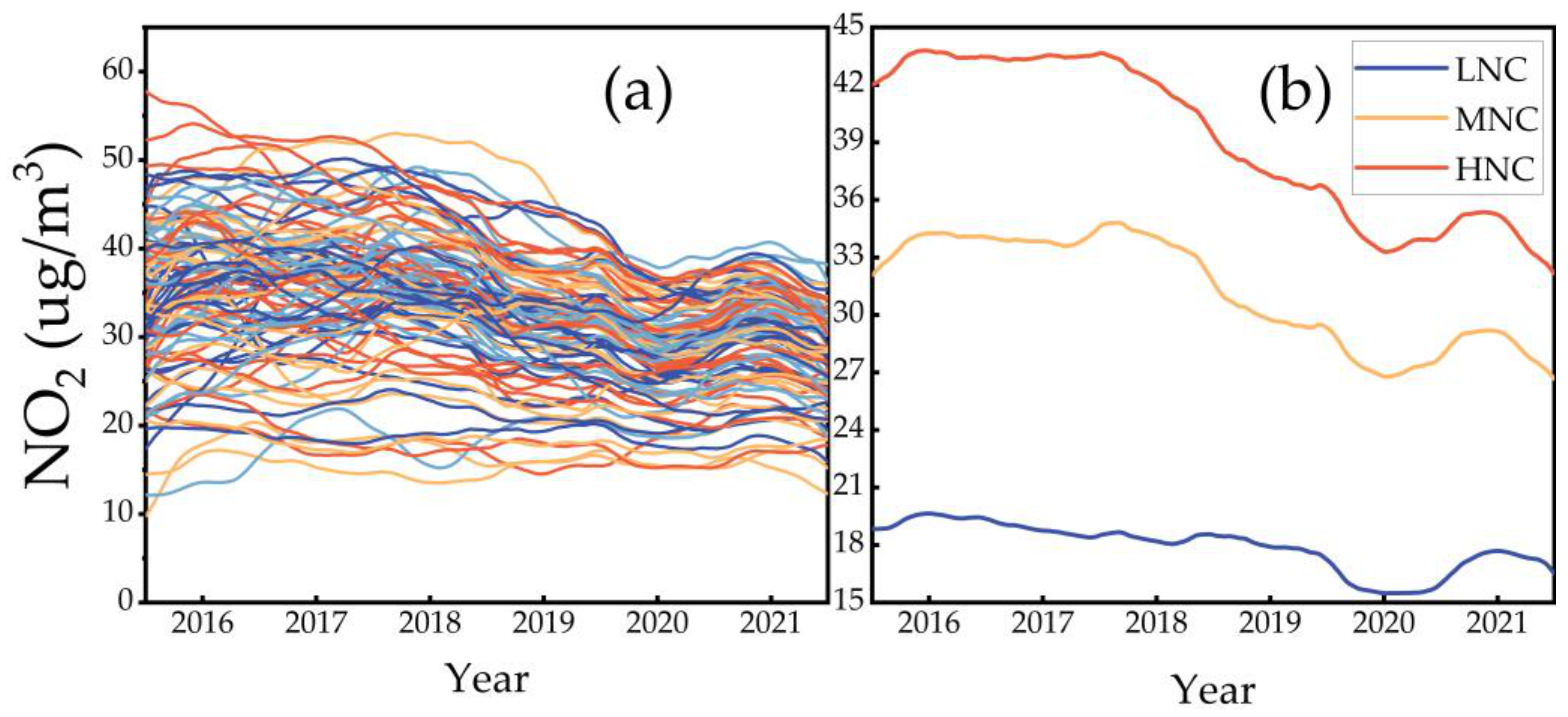
Figure 2a shows a 365-day sliding average of hourly data from 100 cities. Figure 2b displays the curves representing the three types of cities: low NO2 concentration cities (LNC), medium NO2 concentration cities (MNC), and high NO2 concentration cities (HNC), based on their respective NO2 concentrations. The observed “U” change in NO2 concentrations from late 2019 to the first half of 2020 can account for the outbreak of COVID-19 at the end of 2019. This significantly reduced NO2 emissions from public transport and industrial sources during the first half of 2020. Consequently, the gradual resumption of production and work increased NO2 concentrations [38].
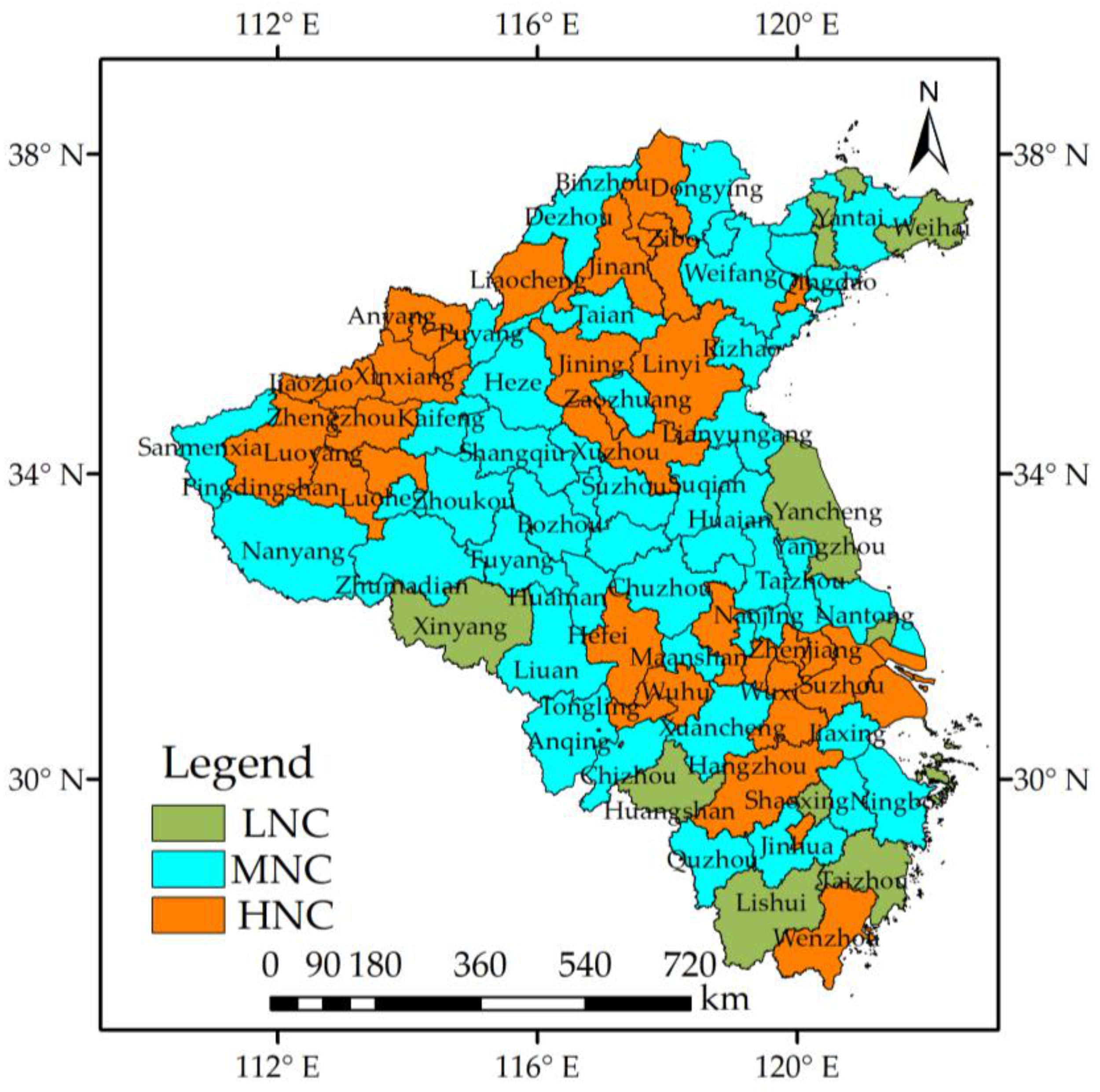
The spatial distribution of the three city types is presented in Figure 3, comprising 15 cities in the LNC, 51 cities in the MNC, and 34 cities in the HNC. The LNC cities primarily consist of popular tourist locations such as Weihai and Huangshan, known for their robust tourism industries, picturesque landscapes, and good air quality. In contrast, the HNC encompasses major cities such as Shanghai, Nanjing, and Hefei alongside cities characterized by a robust industrial presence. The MNC category falls between the LNC and HNC categories.
3.2. Spatial and Temporal Trends in NO2 Concentrations
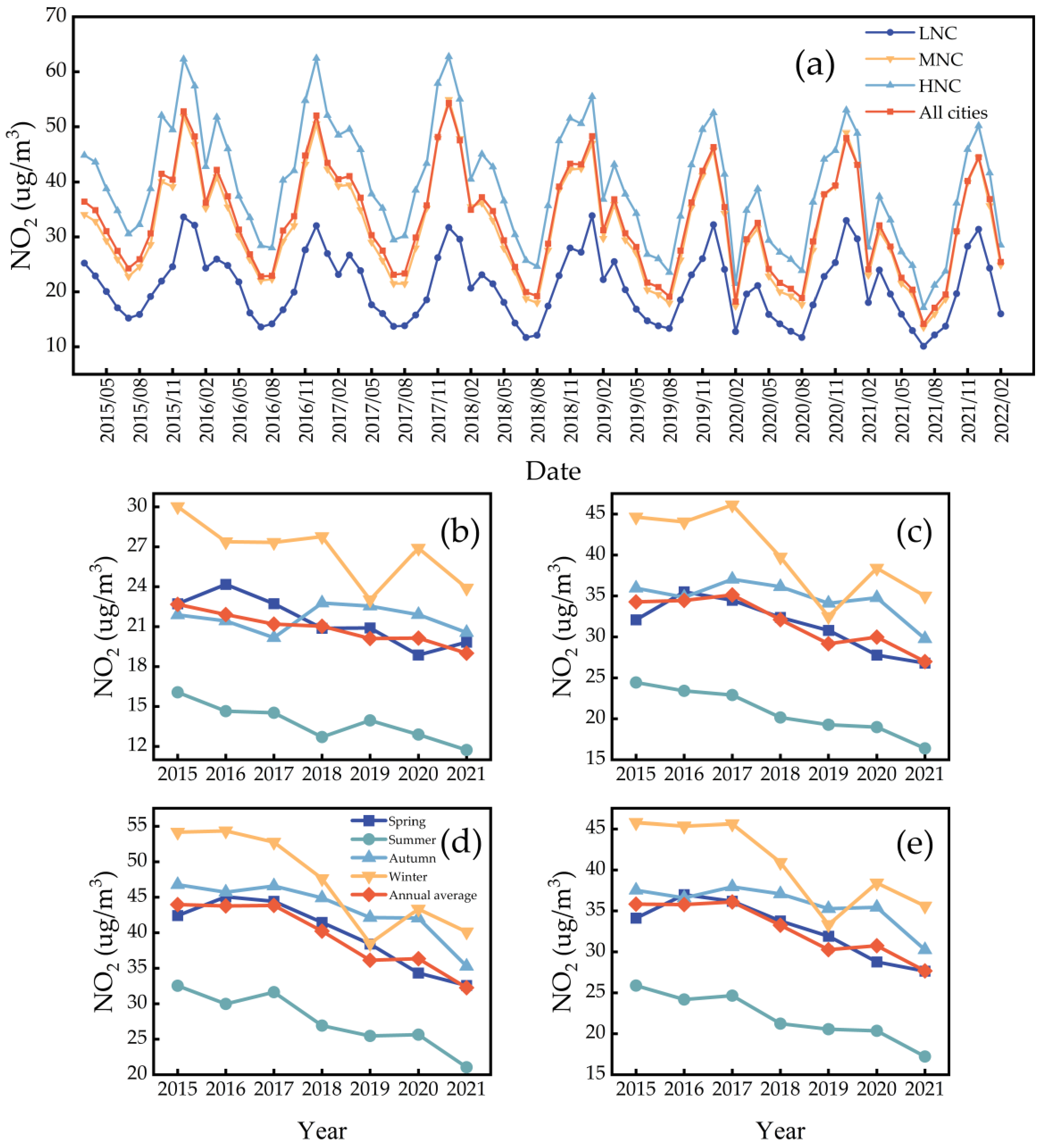
Figure 4 shows the trends in (a) monthly mean NO2 concentrations across various city types and highlights the seasonal characteristics of (b) LNC, (c) MNC, (d) HNC, and (e) ALL. To describe seasonal variations, this study categorizes March to May, June to August, September to November, and December to February as spring, summer, autumn, and winter, respectively. Figure 4a demonstrates a distinct “V” cycle of NO2 concentrations in all types of cities. The months of July and August exhibit the lowest NO2 concentrations, while December is usually the highest of the year. March shows a clear rise in NO2 concentrations annually, known as the “tidal phenomenon” [39]. This phenomenon entails a substantial decline in NO2 concentrations during the Chinese New Year, followed by a subsequent rebound after the festival. The NO2 concentration reaches its highest level in winter, lowest in summer, and slightly higher in autumn compared to spring (Figure 4b). The average NO2 concentration during the summer was 51.8%, 51.9%, 58.4%, and 54.1% of the winter concentration in the three city categories and overall, respectively. From 2015 to 2021, the average NO2 concentration in the three city categories decreased by 16.2%, 21.3%, and 26.7%, respectively, while the overall decrease was 22.7% for all cities. In recent years, the Chinese government has implemented a series of policies to improve air quality, including the Action Plan for Prevention and Control of Air Pollution (https://www.mee.gov.cn/zcwj/gwywj/201811/t20181129_676555.shtml, accessed on 1 February 2023) and the Three-year Action Plan to Fight Air Pollution (https://www.mee.gov.cn/zcwj/gwywj/201807/t20180704_446068.shtml, accessed on 1 February 2023). These policies have led to significant improvements in China’s overall air quality. The improvements can be attributed to several factors, such as the restructuring of industries in different regions, the increased adoption of cleaner energy sources, and the elimination of outdated production capacity, among other reasons.
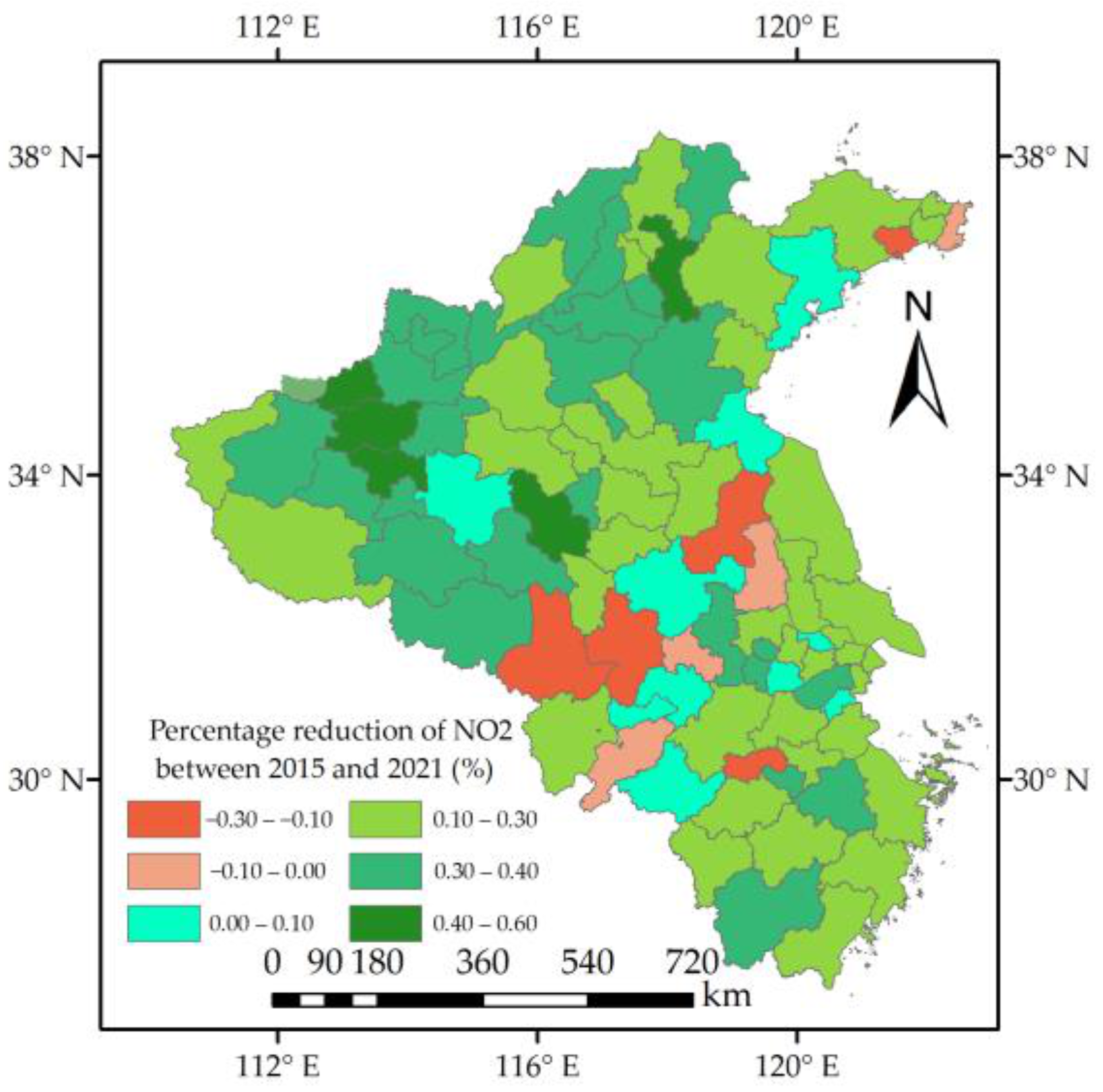
Figure 5 presents the percentage change in NO2 concentrations from 2015 to 2021. Most cities observed a decrease in NO2 concentrations exceeding 10%, and approximately 30% of places witnessed a decline of more than 30%. Bozhou City recorded the most substantial decline in NO2 concentrations at 50.5%. However, a few cities exhibited an increase in NO2 concentrations, with Luan City experiencing an increase of 29.5%. Bozhou, characterized by a well-established kiln industry, numerous enterprises employing boilers, and residents engaging in straw burning, has responded to national and local government policies by conducting an extensive optimization and environmentally conscious transformation of its kiln sector. The city has also enhanced the comprehensive utilization of straw among its population, resulting in a notable reduction in local NOx concentrations. Conversely, Luan grapples with challenges pertaining to the management of pollutant emissions. Primarily originating from the iron and steel, glass, brick and tile, and building materials industries, the ongoing expansion of these sectors has gradually heightened NOx emissions. This underscores the persistent necessity for refining the industrial structure and transitioning to cleaner energy sources.
3.3. Model Results
3.3.1. Model Parameter Results
Since the trends in NO2 concentrations are the same for the three types of cities, the focus of this study is on their overall analysis using a model. Before model fitting, examining the covariance relationship among different variables is essential. Typically, a variance inflation factor (VIF) >10 indicates substantial multicollinearity between variables, which can significantly impact the model results. The test results are presented in Table 2. The VIF for the chosen economic components is all less than 10, suggesting the absence of significant multicollinearity among the variables, aligning with the requirements for GTWR model construction. When comparing the goodness of fit between the GWR and GTWR models, it becomes evident that the GTWR model exhibits a significantly higher R2 than the GWR model. With the Akaike information criterion (AICC) serving as the model goodness-of-fit indicator, the GTWR model demonstrates a lower AICC value than the GWR model, and the residual sum of squares (RSS) for the GWR model exceeds that of the GTWR model, indicating superior goodness of fit for the GTWR model.
3.3.2. The Influence of Social Factors on Urban NO2 Concentrations
Table 3 displays the distribution of coefficient estimates in the GTWR model, encompassing the minimum, lower quartile, median, upper quartile, and maximum values. Each indicator showcases a unique regression coefficient concerning the NO2 concentration in each city. These coefficients exhibit substantial variability, emphasizing variations in influence degrees and associated trends. The positive and negative regression coefficients reveal the dual effects of each indicator on urban NO2, and the varying proportions of positive and negative impacts. This observation suggests spatial instability among the driving factors.
The results of the GTWR indicate that the three types of cities have respective R2 values of 0.741, 0.813, and 0.896, with an overall R2 of 0.802. Furthermore, the coefficients of the GTWR model exhibit overall significance (p < 0.05). Additionally, the results of the GTWR model reveal varying impacts of socioeconomic factors on different types of cities. LNC demonstrates the highest positive correlation with PGDP (1.312) and the strongest negative correlation with the UR rate (−1.430). The highest correlation between EC (0.806) and CV (−0.826) is seen in MNC. Economic factors have a very constant impact on HNC, with PGDP (−0.298) and CV (0.201) having the most effects. These cities had the highest correlation with POP (0.431) and EC (0.520) overall.
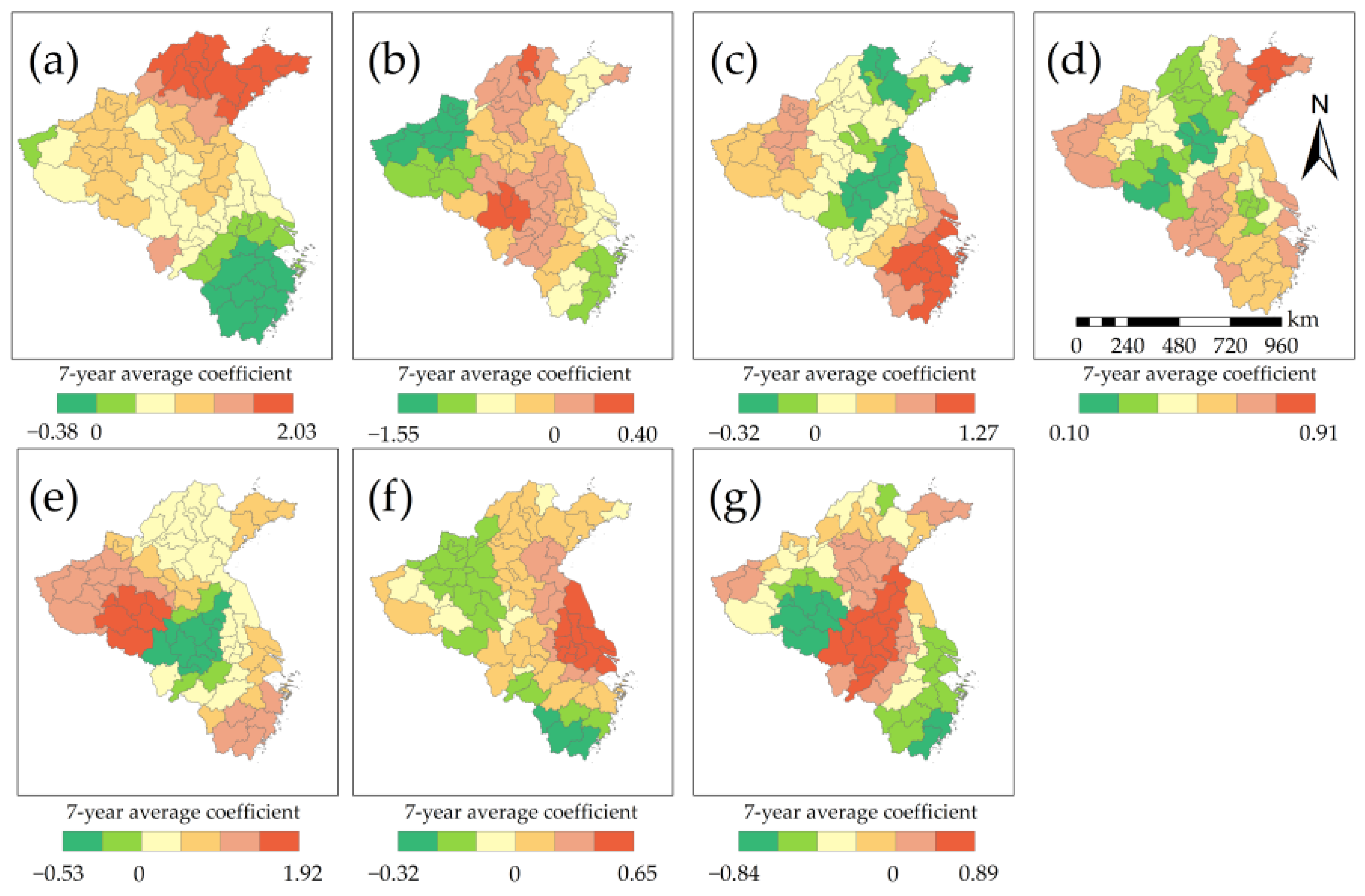
Figure 6 represents the spatial distribution of average coefficients for various drivers in the GTWR model. The results indicate a positive correlation between population density and NO2 concentration in most regions, particularly Shandong Province. Conversely, in some parts of Zhejiang Province, the correlation is negative. Moreover, the correlation between PGDP and NO2 concentration exhibits significant regional variation. Specifically, regions in Zhejiang and Henan primarily display a negative correlation, while in Anhui and Shandong, the correlation is predominantly positive. The recent industrial expansion in Luan and Hefei has, to some extent, led to a significant depletion of resources and energy. This depletion could potentially be a contributing factor to the observed increase in NO2 concentrations within these cities. Zhejiang exhibits the strongest positive correlation with the UR, while the IS positively correlates with NO2 concentrations across all cities in the study area, particularly in Qingdao and Yantai in Shandong, suggesting that the secondary sector is one of the main sources of NO2 emissions. The EC strongly affects urban NO2 emissions in Henan while negatively affecting Anhui Province. The CG shows a negative correlation in certain parts of Henan and Zhejiang, whereas it demonstrates a positive correlation in most cities, particularly in Jiangsu Province. Regarding CV, Anhui Province exhibits a positive correlation, while Henan and Zhejiang primarily display a negative correlation. This finding aligns with the study by Carslaw et al. [40], which reports a decline in traffic-related NO2 concentrations due to upgraded emission standards in the automotive industry, predominantly attributed to reduced diesel vehicle emissions rather than light-duty vehicles. The 2022 Annual Report on Environmental Management of Mobile Sources in China (www.mee.gov.cn/hjzl/sthjzk/ydyhjgl/, accessed on 1 February 2023) confirms a similar trend.
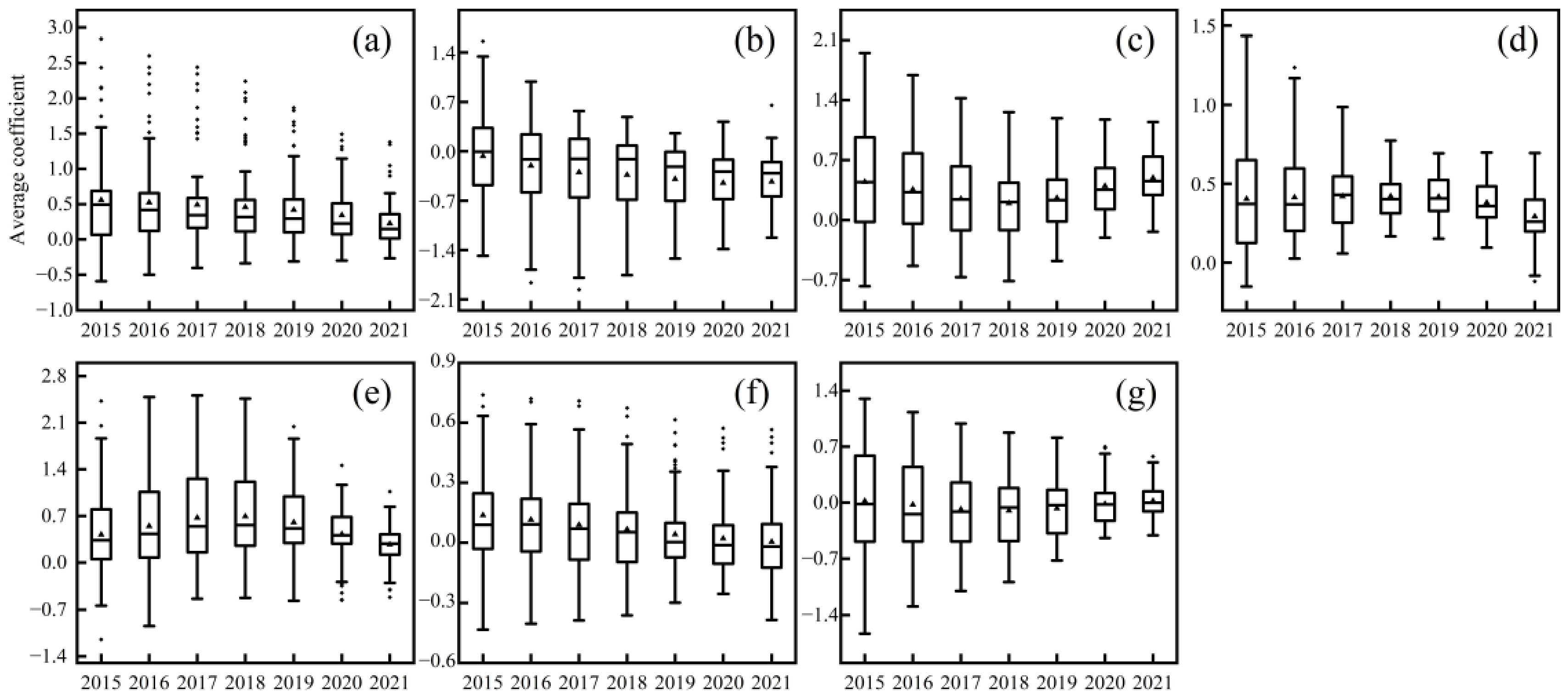
Figure 7 illustrates the temporal distribution of average coefficients for various drivers in the GTWR model. Between 2015 and 2021, POP and CG were positively correlated with NO2 concentrations, diminishing each year, and the negative correlation between PGDP and NO2 concentrations increased. Although economic development can lead to environmental degradation, as income levels rise, environmental issues are expected to improve, leading to reduced pollutant emissions [41], which may be the main reason for the decrease in NO2 concentration in Henan Province. The UR exhibits a “U” trend, implying that urbanization has been exacerbating environmental degradation in recent years [42]. The proportion of the IS and EC indicates an inverted “U” distribution. With the reinforcement of relevant laws and stringent regulations and the continuous adjustment of cleaning policies in recent years, China has been transitioning from a pollution-intensive secondary sector to a tertiary sector characterized by high value-added and advanced technology. This industrial and technological upgrade will help mitigate the negative impact on environmental quality [43].
3.3.3. The Influence of Meteorological Factors on Urban NO2 Concentrations
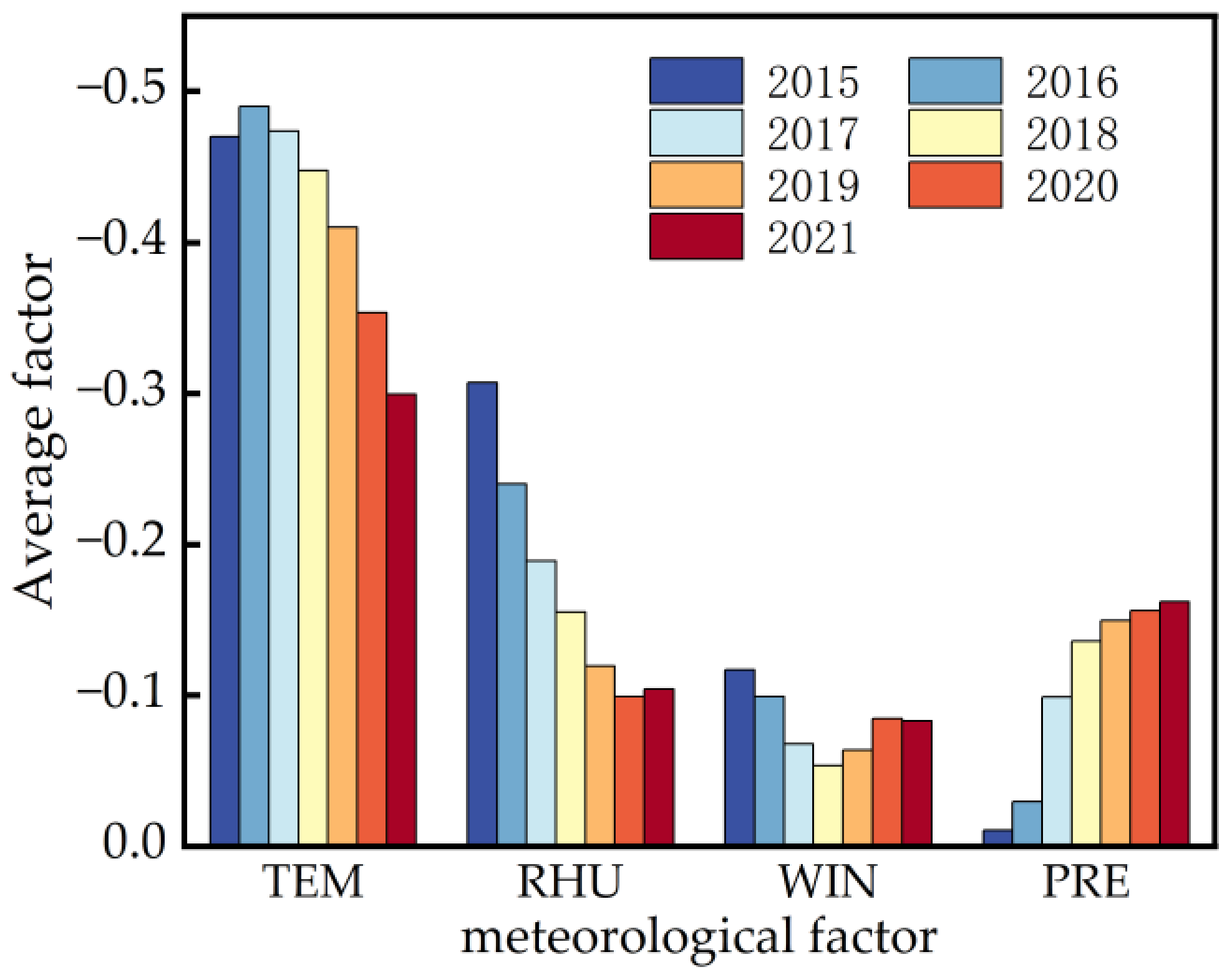
Table 4 presents the results of global simulation coefficients for meteorological factors in the GTWR, and the coefficients of the GTWR model exhibit overall significance (p < 0.05). with an R2 value of 0.831, suggesting a clear relationship between the variables and the variation in NO2 concentration. The results indicate correlations between TEM, RHU, WIN, PRE, and NO2 concentrations, with mean coefficients of −0.411, −0.147, −0.032, and −0.116, respectively. TEM exhibits a significant negative correlation with NO2 concentration, displaying a correlation coefficient of −0.411. The lower quartile (LQ) and upper quartile (UQ) values are −0.502 and −0.344, respectively. As the temperature increases, the photochemical reaction rate of NO2 intensifies [44].
Figure 8 illustrates the annual variations in the mean coefficients of various meteorological factors from 2015 to 2021. The average coefficients for TEM and RHU have generally decreased in recent years. The study found that the inhibitory effect of temperature on NO2 concentration was most significant at lower temperatures and stabilized at higher temperatures. Additionally, NO2 can be effectively removed from the air only when the relative humidity is high [45]. The trend of WIN is decreasing and then increasing; the average coefficient of PRE is increasing year by year, and the increase is most obvious in 2017.
4. Conclusions
In this study, based on hourly NO2 observations from 2015–2021, we classify cities in Mid-Eastern China into three categories by k-means clustering and explore the effects of drivers on spatial and temporal variations in NO2 concentrations using the GTWR model. We concluded that the implementation of air pollution control policies in recent years has led to a reduction in NO2 concentrations in most cities across mid-eastern China, although certain regions in Anhui and Jiangsu experienced exceptions to this trend. Furthermore, we observed a significant decrease in NO2 levels during early 2020, attributed to the impact of COVID-19. Additionally, the seasonal variation in NO2 concentration follows a distinct pattern, being higher in winter and lower in summer.
We carried out extensive data analysis in this paper and obtained some important conclusions. First, the strongest correlations of NO2 concentration are found with POP and EC, which aligns with the consensus among researchers in this field [46,47]. This reaffirms the validity of our findings and underscores the reliability of our methodologies. Second, the relationships of NO2 with socio-economic factors exhibit noticeable variations across different provinces, which contributes valuable insights into the visualization of spatial and temporal variations in the average coefficients of each of the related NO2 concentrations, and future government policies should take into account the characteristics of different regions in formulating new development requirements. In conclusion, the study reveals the link between NO2 concentrations and their possible influences, taking into account geographical differences and temporal dynamics. The empirical findings of this research highlight the unequivocal reality that air pollution challenges vary significantly across diverse Chinese cities. These disparities emerge due to pronounced spatial and temporal variations in the interplay between NO2 concentrations and socioeconomic variables.
This study has the potential to inform government decision-making; however, it also reveals certain limitations that necessitate future research efforts. Primarily, the constraints associated with the NO2 data obtained from meteorological stations hindered the classification of NO2 emission sources, including transport, industry, and heating. Subsequent investigations should endeavor to incorporate more comprehensive and detailed data to facilitate more precise source analysis. Moreover, we selected and standardized seven social factors, which resulted in a smaller distribution of regression coefficients between the different factors. In addition, the complexity of the mechanisms of air pollution formation and comprehending urban NO2 drivers through regression analysis remain challenges. Future research endeavors could employ a combined approach involving correlation analysis and chemical modeling to gain deeper insight into the multifaceted factors influencing NO2 formation.
Author Contributions
Conceptualization, M.Y. and Y.J.; methodology, Y.J.; software, M.Y. and Y.J.; validation, M.Y., Y.J. and Q.Z.; formal analysis, M.Y. and Y.J.; investigation, Y.J. and Y.L.; data curation, Y.J., J.Q. and Y.L.; writing—original draft preparation, Y.J.; writing—review and editing, M.Y.; visualization, Y.J.; supervision, M.Y.; project administration, M.Y.; funding acquisition, M.Y. All authors have read and agreed to the published version of the manuscript.
Funding
This study was funded by the Research Foundation of Anhui Jianzhu University (2020QDZ31), the Anhui Provincial Key Laboratory of Environmental Pollution Control and Resource Reuse (2022EPC07), and the National Natural Science Foundation of China (41005016, 41105031).
Institutional Review Board Statement
Not applicable.
Informed Consent Statement
Not applicable.
Data Availability Statement
Hourly NO2 observations were collected from the China National Environmental Monitoring Platform (http://106.37.208.233:20035/, accessed on 1 February 2023). Socioeconomic factor data were acquired from the National Statistical Database and the provincial and prefectural statistical yearbooks from 2015 to 2021. The meteorological data are from the National Centers for Environmental Information (https://www.ncei.noaa.gov/, accessed on 1 February 2023).
Acknowledgments
We want to express our sincere gratitude to the anonymous reviewers and editors for their efforts in improving the paper.
Conflicts of Interest
The authors declare no conflict of interest.
References
- Zhang, L.; Wang, Y.; Feng, C.; Liang, S.; Liu, Y.; Du, H.; Jia, N. Understanding the industrial NOx and SO2 pollutant emissions in China from sector linkage perspective. Sci. Total Environ. 2021, 770, 145242. [Google Scholar] [CrossRef] [PubMed]
- Fan, M.-Y.; Zhang, Y.-L.; Lin, Y.-C.; Li, L.; Xie, F.; Hu, J.; Mozaffar, A.; Cao, F. Source apportionments of atmospheric volatile organic compounds in Nanjing, China during high ozone pollution season. Chemosphere 2021, 263, 128025. [Google Scholar] [CrossRef] [PubMed]
- Li, W.; Qi, Y.; Qu, W.; Qu, W.; Shi, J.; Zhang, D.; Liu, Y.; Zhang, Y.; Zhang, W.; Ren, D.; et al. PM2.5 source apportionment identified with total and soluble elements in positive matrix factorization. Sci. Total Environ. 2023, 858, 159948. [Google Scholar] [CrossRef] [PubMed]
- Guan, W.-J.; Zheng, X.-Y.; Chung, K.F.; Zhong, N.-S. Impact of air pollution on the burden of chronic respiratory diseases in China: Time for urgent action. Lancet 2016, 388, 1939–1951. [Google Scholar] [CrossRef]
- Xue, Y.; Wang, L.; Zhang, Y.; Zhao, Y.; Liu, Y. Air pollution: A culprit of lung cancer. J. Hazard. Mater. 2022, 434, 128937. [Google Scholar] [CrossRef] [PubMed]
- Buoli, M.; Grassi, S.; Caldiroli, A.; Carnevali, G.S.; Mucci, F.; Iodice, S.; Cantone, L.; Pergoli, L.; Bollati, V. Is there a link between air pollution and mental disorders? Environ. Int. 2018, 118, 154–168. [Google Scholar] [CrossRef]
- Deng, Q.; Lu, C.; Norbäck, D.; Bornehag, C.-G.; Zhang, Y.; Liu, W.; Yuan, H.; Sundell, J. Early life exposure to ambient air pollution and childhood asthma in China. Environ. Res. 2015, 143, 83–92. [Google Scholar] [CrossRef]
- Itahashi, S.; Ge, B.; Sato, K.; Fu, J.S.; Wang, X.; Yamaji, K.; Nagashima, T.; Li, J.; Kajino, M.; Liao, H.; et al. MICS-Asia III: Overview of model intercomparison and evaluation of acid deposition over Asia. Atmos. Chem. Phys. 2020, 20, 2667–2693. [Google Scholar] [CrossRef]
- Silvern, R.F.; Jacob, D.J.; Mickley, L.J.; Sulprizio, M.P.; Travis, K.R.; Marais, E.A.; Cohen, R.C.; Laughner, J.L.; Choi, S.; Joiner, J.; et al. Using satellite observations of tropospheric NO2 columns to infer long-term trends in US NOx emissions: The importance of accounting for the free tropospheric NO2 background. Atmos. Chem. Phys. 2019, 19, 8863–8878. [Google Scholar] [CrossRef]
- Huang, G.; Sun, K. Non-negligible impacts of clean air regulations on the reduction of tropospheric NO2 over East China during the COVID-19 pandemic observed by OMI and TROPOMI. Sci. Total Environ. 2020, 745, 141023. [Google Scholar] [CrossRef]
- Zheng, C.; Zhao, C.; Li, Y.; Wu, X.; Zhang, K.; Gao, J.; Qiao, Q.; Ren, Y.; Zhang, X.; Chai, F. Spatial and temporal distribution of NO2 and SO2 in Inner Mongolia urban agglomeration obtained from satellite remote sensing and ground observations. Atmos. Environ. 2018, 188, 50–59. [Google Scholar] [CrossRef]
- De Hoogh, K.; Saucy, A.; Shtein, A.; Schwartz, J.; West, E.A.; Strassmann, A.; Puhan, M.; Röösli, M.; Stafoggia, M.; Kloog, I. Predicting Fine-Scale Daily NO2 for 2005–2016 Incorporating OMI Satellite Data Across Switzerland. Environ. Sci. Technol. 2019, 53, 10279–10287. [Google Scholar] [CrossRef] [PubMed]
- Bechle, M.J.; Millet, D.B.; Marshall, J.D. Remote sensing of exposure to NO2: Satellite versus ground-based measurement in a large urban area. Atmos. Environ. 2013, 69, 345–353. [Google Scholar] [CrossRef]
- Hůnová, I.; Bäumelt, V.; Modlík, M. Long-term trends in nitrogen oxides at different types of monitoring stations in the Czech Republic. Sci. Total Environ. 2020, 699, 134378. [Google Scholar] [CrossRef]
- Shen, Y.; Jiang, F.; Feng, S.; Xia, Z.; Zheng, Y.; Lyu, X.; Zhang, L.; Lou, C. Increased diurnal difference of NO2 concentrations and its impact on recent ozone pollution in eastern China in summer. Sci. Total Environ. 2023, 858, 159767. [Google Scholar] [CrossRef]
- Cui, Y.; Zha, H.; Dang, Y.; Qiu, L.; He, Q.; Jiang, L. Spatio-Temporal Heterogeneous Impacts of the Drivers of NO2 Pollution in Chinese Cities: Based on Satellite Observation Data. Remote Sens. 2022, 14, 3487. [Google Scholar] [CrossRef]
- Zheng, B.; Zhang, Q.; Geng, G.; Chen, C.; Shi, Q.; Cui, M.; Lei, Y.; He, K. Changes in China’s anthropogenic emissions and air quality during the COVID-19 pandemic in 2020. Earth Syst. Sci. Data 2021, 13, 2895–2907. [Google Scholar] [CrossRef]
- Li, R.; Wang, Z.; Cui, L.; Fu, H.; Zhang, L.; Kong, L.; Chen, W.; Chen, J. Air pollution characteristics in China during 2015–2016: Spatiotemporal variations and key meteorological factors. Sci. Total Environ. 2019, 648, 902–915. [Google Scholar] [CrossRef]
- Yang, J.; Ji, Z.; Kang, S.; Zhang, Q.; Chen, X.; Lee, S.-Y. Spatiotemporal variations of air pollutants in western China and their relationship to meteorological factors and emission sources. Environ. Pollut. 2019, 254, 112952. [Google Scholar] [CrossRef]
- Xu, B.; Zhong, R.; Liu, D.; Liu, Y. Investigating the impact of energy consumption and nitrogen fertilizer on NOx emissions in China based on the environmental Kuznets curve. Environ. Dev. Sustain. 2021, 23, 17590–17605. [Google Scholar] [CrossRef]
- Wang, J.; Ma, Y.; Qiu, Y.; Liu, L.; Dong, Z. Spatially differentiated effects of socioeconomic factors on China’s NOx generation from energy consumption: Implications for mitigation policy. J. Environ. Manag. 2019, 250, 109417. [Google Scholar] [CrossRef] [PubMed]
- Wang, J.; Qiu, Y.; He, S.; Liu, N.; Xiao, C.; Liu, L. Investigating the driving forces of NOx generation from energy consumption in China. J. Clean. Prod. 2018, 184, 836–846. [Google Scholar] [CrossRef]
- Wang, J.; Li, X.; Ding, S.; Xu, X.; Liu, L.; Dong, L.; Feng, Y. Uncovering temporal-spatial drivers of vehicular NOx emissions in China. J. Clean. Prod. 2021, 288, 125635. [Google Scholar] [CrossRef]
- Xu, Y.; Zhang, W.; Huo, T.; Streets, D.G.; Wang, C. Investigating the spatio-temporal influences of urbanization and other socioeconomic factors on city-level industrial NOx emissions: A case study in China. Environ. Impact Assess. Rev. 2023, 99, 106998. [Google Scholar] [CrossRef]
- Zhang, G.; Han, J.; Su, B. Contributions of cleaner production and end-of-pipe treatment to NOx emissions and intensity reductions in China, 1997–2018. J. Environ. Manag. 2023, 326, 116822. [Google Scholar] [CrossRef] [PubMed]
- He, S.; Zhao, L.; Ding, S.; Liang, S.; Dong, L.; Wang, J.; Feng, Y.; Liu, L. Mapping economic drivers of China’s NOx emissions due to energy consumption. J. Clean. Prod. 2019, 241, 118130. [Google Scholar] [CrossRef]
- Enkhbat, E.; Geng, Y.; Zhang, X.; Jiang, H.; Liu, J.; Wu, D. Driving Forces of Air Pollution in Ulaanbaatar City Between 2005 and 2015: An Index Decomposition Analysis. Sustainability 2020, 12, 3185. [Google Scholar] [CrossRef]
- Guo, S.; Liu, G.; Liu, S. Driving factors of NOX emission reduction in China’s power industry: Based on LMDI decomposition model. Environ. Sci. Pollut. Res. 2023, 30, 51042–51060. [Google Scholar] [CrossRef]
- Liu, X.; Yi, G.; Zhou, X.; Zhang, T.; Lan, Y.; Yu, D.; Wen, B.; Hu, J. Atmospheric NO2 Distribution Characteristics and Influencing Factors in Yangtze River Economic Belt: Analysis of the NO2 Product of TROPOMI/Sentinel-5P. Atmosphere 2021, 12, 1142. [Google Scholar] [CrossRef]
- Yang, L.; Qin, C.; Li, K.; Deng, C.; Liu, Y. Quantifying the Spatiotemporal Heterogeneity of PM2.5 Pollution and Its Determinants in 273 Cities in China. IJERPH 2023, 20, 1183. [Google Scholar] [CrossRef]
- Huang, B.; Wu, B.; Barry, M. Geographically and temporally weighted regression for modeling spatio-temporal variation in house prices. Int. J. Geogr. Inf. Sci. 2010, 24, 383–401. [Google Scholar] [CrossRef]
- Chen, Y.; Chen, M.; Huang, B.; Wu, C.; Shi, W. Modeling the Spatiotemporal Association Between COVID-19 Transmission and Population Mobility Using Geographically and Temporally Weighted Regression. GeoHealth 2021, 5, e2021GH000402. [Google Scholar] [CrossRef] [PubMed]
- Zhao, M.; Wang, H.; Sun, J.; Tang, R.; Cai, B.; Song, X.; Huang, X.; Huang, J.; Fan, Z. Spatio-temporal characteristics of soil Cd pollution and its influencing factors: A Geographically and temporally weighted regression (GTWR) method. J. Hazard. Mater. 2023, 446, 130613. [Google Scholar] [CrossRef]
- Zhang, W.; Wang, J.; Xu, Y.; Wang, C.; Streets, D.G. Analyzing the spatio-temporal variation of the CO2 emissions from district heating systems with “Coal-to-Gas” transition: Evidence from GTWR model and satellite data in China. Sci. Total Environ. 2022, 803, 150083. [Google Scholar] [CrossRef]
- GB 3095-2012; Ambient Air Quality Standards. Ministry of Environmental Protection of PRC: Beijing, China, 2012.
- Ikotun, A.M.; Ezugwu, A.E.; Abualigah, L.; Abuhaija, B.; Heming, J. K-means clustering algorithms: A comprehensive review, variants analysis, and advances in the era of big data. Inf. Sci. 2023, 622, 178–210. [Google Scholar] [CrossRef]
- Brunsdon, C.; Fotheringham, A.S.; Charlton, M.E. Geographically Weighted Regression: A Method for Exploring Spatial Nonstationarity. Geogr. Anal. 1996, 28, 281–298. [Google Scholar] [CrossRef]
- Wang, Z.; Uno, I.; Yumimoto, K.; Itahashi, S.; Chen, X.; Yang, W.; Wang, Z. Impacts of COVID-19 lockdown, Spring Festival and meteorology on the NO2 variations in early 2020 over China based on in-situ observations, satellite retrievals and model simulations. Atmos. Environ. 2021, 244, 117972. [Google Scholar] [CrossRef]
- Li, D.; Wu, Q.; Wang, H.; Xiao, H.; Xu, Q.; Wang, L.; Feng, J.; Yang, X.; Cheng, H.; Wang, L.; et al. The Spring Festival Effect: The change in NO2 column concentration in China caused by the migration of human activities. Atmos. Pollut. Res. 2021, 12, 101232. [Google Scholar] [CrossRef]
- Carslaw, D.C.; Murrells, T.P.; Andersson, J.; Keenan, M. Have vehicle emissions of primary NO2 peaked? Faraday Discuss. 2016, 189, 439–454. [Google Scholar] [CrossRef]
- Ding, Y.; Zhang, M.; Chen, S.; Wang, W.; Nie, R. The environmental Kuznets curve for PM2.5 pollution in Beijing-Tianjin-Hebei region of China: A spatial panel data approach. J. Clean. Prod. 2019, 220, 984–994. [Google Scholar] [CrossRef]
- Zhu, Y.; Zhan, Y.; Wang, B.; Li, Z.; Qin, Y.; Zhang, K. Spatiotemporally mapping of the relationship between NO2 pollution and urbanization for a megacity in Southwest China during 2005–2016. Chemosphere 2019, 220, 155–162. [Google Scholar] [CrossRef] [PubMed]
- Liu, F.; Zhang, Q.; van der A, R.; Zheng, B.; Tong, D.; Yan, L.; Zheng, Y.; He, K. Recent reduction in NO x emissions over China: Synthesis of satellite observations and emission inventories. Environ. Res. Lett. 2016, 11, 114002. [Google Scholar] [CrossRef]
- Wang, C.; Wang, T.; Wang, P. The Spatial–Temporal Variation of Tropospheric NO2 over China during 2005 to 2018. Atmosphere 2019, 10, 444. [Google Scholar] [CrossRef]
- Ju, T.; Geng, T.; Li, B.; An, B.; Huang, R.; Fan, J.; Liang, Z.; Duan, J. Impacts of Certain Meteorological Factors on Atmospheric NO2 Concentrations during COVID-19 Lockdown in 2020 in Wuhan, China. Sustainability 2022, 14, 16720. [Google Scholar] [CrossRef]
- Zhan, D.; Kwan, M.-P.; Zhang, W.; Wang, S.; Yu, J. Spatiotemporal Variations and Driving Factors of Air Pollution in China. IJERPH 2017, 14, 1538. [Google Scholar] [CrossRef]
- Wang, L.; Wang, Y.; He, H.; Lu, Y.; Zhou, Z. Driving force analysis of the nitrogen oxides intensity related to electricity sector in China based on the LMDI method. J. Clean. Prod. 2020, 242, 118364. [Google Scholar] [CrossRef]
Figure 1.
Mid-Eastern China and its monitoring site distribution.

Figure 2.
Sliding average (a) and k-means cluster analysis results (b). In (a), each line represents a different city.
Figure 2.
Sliding average (a) and k-means cluster analysis results (b). In (a), each line represents a different city.

Figure 3.
Spatial distribution of the three types of cities.

Figure 4.
The monthly and seasonal distributions of NO2 concentrations from 2015 to 2021. (a) Month changes in different types of cities; (b) LNC; (c) MNC; (d) HNC and (e) all city annual trends in NO2 concentrations.
Figure 4.
The monthly and seasonal distributions of NO2 concentrations from 2015 to 2021. (a) Month changes in different types of cities; (b) LNC; (c) MNC; (d) HNC and (e) all city annual trends in NO2 concentrations.

Figure 5.
Percentage reduction in NO2 concentration between 2015 and 2021.

Figure 6.
Spatial distribution of (a) POP, (b) PGDP, (c) UR, (d) IS, (e) EC, (f) CG, and (g) CV coefficients in the GTWR model.
Figure 6.
Spatial distribution of (a) POP, (b) PGDP, (c) UR, (d) IS, (e) EC, (f) CG, and (g) CV coefficients in the GTWR model.

Figure 7.
Temporal distribution of (a) POP, (b) PGDP, (c) UR, (d) IS, (e) EC, (f) CG, and (g) CV coefficients in the GTWR model.
Figure 7.
Temporal distribution of (a) POP, (b) PGDP, (c) UR, (d) IS, (e) EC, (f) CG, and (g) CV coefficients in the GTWR model.

Figure 8.
Annual variation in the mean coefficients of meteorological factors.


Table 1.
Statistical description of each variable used in the GTWR model.
| Variable | Unit | ||
|---|---|---|---|
| socioeconomic factors | POP | Permanent population density | 10,000 Capita/km2 |
| PGDP | GDP per capita | yuan | |
| UR | Urbanization rate | % | |
| IS | Share of secondary sector output in total GDP | % | |
| EC | Electricity consumption of the whole society | kwh | |
| CG | Coverage rate of urban green areas | % | |
| CV | Civil car vehicles | car | |
| meteorological factors | TEM | Average temperatures | °C |
| RHU | Relative humidity | % | |
| WIN | Average wind speed | m/s | |
| PRE | Average precipitation | mm |
Table 2.
Descriptive statistics of regression results of GWR and GTWR models.
| LNC | MNC | HNC | ALL | Meteorological | ||
|---|---|---|---|---|---|---|
| VIF | 3.15–9.17 | 1.19–9.10 | 1.35–6.68 | 1.25–5.29 | 1.56–8.35 | |
| Bandwidth | GWR | 1.987 | 0.115 | 0.115 | 0.115 | 0.115 |
| GTWR | 0.297 | 0.113 | 0.137 | 0.115 | 0.115 | |
| RSS | GWR | 29.310 | 103.427 | 53.258 | 175.326 | 98.54 |
| GTWR | 12.678 | 53.389 | 18.978 | 102.387 | 89.667 | |
| AICC | GWR | 138.032 | 689.429 | 400.41 | 1062.62 | 943.56 |
| GTWR | 137.187 | 614.578 | 365.268 | 947.706 | 824.84 | |
| R2 | GWR | 0.402 | 0.638 | 0.707 | 0.662 | 0.795 |
| GTWR | 0.741 | 0.813 | 0.896 | 0.802 | 0.831 |
Table 3.
Results for social factors in the GTWR model.
| Type of City | Min. | LQ | Med. | UQ | Max. | ||
|---|---|---|---|---|---|---|---|
| POP | Permanent population density | LNC | −2.339 | −1.088 | −0.573 | −0.033 | 0.002 |
| MNC | −1.294 | 0.011 | 0.122 | 0.303 | 1.078 | ||
| HNC | −1.482 | −0.328 | −0.119 | 0.111 | 1.047 | ||
| ALL | −0.593 | 0.076 | 0.431 | 0.581 | 2.842 | ||
| PGDP | GDP per capita | LNC | 0.050 | 0.116 | 1.312 | 2.474 | 5.271 |
| MNC | −6.644 | −0.938 | −0.467 | 0.196 | 5.333 | ||
| HNC | −2.356 | −1.076 | −0.298 | 0.239 | 1.993 | ||
| ALL | −1.962 | −0.645 | −0.311 | 0.054 | 1.560 | ||
| UR | Urbanization rate | LNC | −4.173 | −2.292 | −1.430 | −0.502 | −0.421 |
| MNC | −2.616 | −0.356 | 0.181 | 0.592 | 6.396 | ||
| HNC | −2.054 | −0.274 | 0.065 | 0.546 | 1.316 | ||
| ALL | −7.773 | 0.016 | 0.342 | 0.650 | 1.949 | ||
| IS | Share of secondary sector output in total GDP | LNC | −0.705 | −0.232 | 0.035 | 0.309 | 0.578 |
| MNC | −1.095 | 0.013 | 0.248 | 0.518 | 1.774 | ||
| HNC | −0.745 | −0.108 | 0.158 | 0.399 | 1.331 | ||
| ALL | −0.151 | 0.252 | 0.393 | 0.516 | 1.436 | ||
| EC | Electricity consumption of the whole society | LNC | −0.598 | −0.158 | 0.241 | 0.688 | 0.781 |
| MNC | −1.934 | −0.288 | 0.806 | 1.847 | 7.706 | ||
| HNC | −0.769 | −0.197 | 0.147 | 0.457 | 2.118 | ||
| ALL | −1.148 | 0.168 | 0.520 | 0.840 | 2.508 | ||
| CG | Coverage rate of urban green areas | LNC | −1.660 | −0.798 | −0.540 | −0.198 | −0.141 |
| MNC | −0.534 | −0.062 | 0.101 | 0.228 | 1.366 | ||
| HNC | −0.754 | −0.312 | −0.073 | 0.104 | 0.409 | ||
| ALL | −0.433 | −0.082 | 0.068 | 0.170 | 0.739 | ||
| CV | Civil car vehicles | LNC | −0.402 | −0.249 | 0.261 | 0.515 | 1.820 |
| MNC | −6.679 | −2.100 | −0.826 | 0.223 | 1.689 | ||
| HNC | −1.965 | −0.240 | 0.201 | 0.657 | 1.970 | ||
| ALL | −1.634 | −0.357 | −0.036 | 0.210 | 1.299 |
Table 4.
Results for meteorological factors in the GTWR model.
| Min. | LQ | Med. | UQ | Max. | |
|---|---|---|---|---|---|
| TEM | −0.951 | −0.502 | −0.411 | −0.344 | −0.064 |
| RHU | −0.295 | −0.251 | −0.147 | −0.022 | 0.479 |
| WIN | −0.804 | −0.417 | −0.032 | 0.235 | 0.682 |
| PRE | −0.588 | −0.241 | −0.116 | −0.007 | 0.714 |
Disclaimer/Publisher’s Note: The statements, opinions and data contained in all publications are solely those of the individual author(s) and contributor(s) and not of MDPI and/or the editor(s). MDPI and/or the editor(s) disclaim responsibility for any injury to people or property resulting from any ideas, methods, instructions or products referred to in the content. |
© 2023 by the authors. Licensee MDPI, Basel, Switzerland. This article is an open access article distributed under the terms and conditions of the Creative Commons Attribution (CC BY) license (https://creativecommons.org/licenses/by/4.0/).
Share and Cite
MDPI and ACS Style
Yi, M.; Jiang, Y.; Zhao, Q.; Qiu, J.; Li, Y. Spatiotemporal Variation and Driving Factors for NO2 in Mid-Eastern China. Atmosphere 2023, 14, 1369. https://doi.org/10.3390/atmos14091369
AMA Style
Yi M, Jiang Y, Zhao Q, Qiu J, Li Y. Spatiotemporal Variation and Driving Factors for NO2 in Mid-Eastern China. Atmosphere. 2023; 14(9):1369. https://doi.org/10.3390/atmos14091369
Chicago/Turabian StyleYi, Mingjian, Yongqing Jiang, Qiang Zhao, Junxia Qiu, and Yi Li. 2023. "Spatiotemporal Variation and Driving Factors for NO2 in Mid-Eastern China" Atmosphere 14, no. 9: 1369. https://doi.org/10.3390/atmos14091369
Note that from the first issue of 2016, this journal uses article numbers instead of page numbers. See further details here.