Responses to the Preparation of the 2021 M7.4 Madoi Earthquake in the Lithosphere–Atmosphere–Ionosphere System

Abstract

The purpose of this work is to investigate the responses of multiple parameters to the Madoi earthquake preparation. A new method is employed to extract anomalies in a geomagnetic field. The results show that there were abnormal changes in the lithosphere, atmosphere, and ionosphere near the epicenter before the earthquake. Despite the differences in spatial and temporal resolutions, the increase in geomagnetic residuals in the lithosphere exhibits similar temporal characteristics to the enhancement of thermal infrared radiation in the atmosphere. Two high–value regions are present in the ground–based geomagnetic high residuals and the ionospheric disturbances. The northern one is around the epicenter of the Madoi earthquake. Near the southern one, an M6.4 Yangbi earthquake occurred four hours before the Madoi earthquake. In this study, we have observed almost all of the physical phenomena that can occur during the preparation of an earthquake, as predicted using the electrostatic channel model. It can be inferred that the electrostatic channel is a possible mechanism for coupling between the lithosphere, atmosphere, and ionosphere during the Madoi earthquake.

1. Introduction

The discovery that local high–amplitude ULF signals were observed near the epicenters of violent M > 7.0 earthquakes at Loma Prieta [1] and Spitak [2,3] is the first milestone in the field of seismo–electromagnetics. Various ground–based or satellite observations in recent decades have proven that earthquakes can cause disturbances in the atmosphere and ionosphere [4,5,6,7,8]. The possible relationship between earthquakes and electromagnetic/ionospheric disturbances has received extensive attention in the past 20 years, especially after the 2008 Wenchuan earthquake [9,10,11]. Researchers also utilize satellite remote sensing data, which covers numerous seismic regions, to investigate thermal anomalies related to earthquakes [12,13,14,15,16,17,18,19,20]. To investigate the mechanisms by which earthquakes induce disturbances in the atmosphere and ionosphere, scientists have put forth various models that describe the coupling between the lithosphere, atmosphere, and ionosphere [21,22,23]. Hayakawa [24,25] has proposed several possible hypotheses regarding the mechanism of LAIC, including the chemical channel [26,27], acoustic channel [28,29], and electromagnetic channel [30,31]. Some scientists consider the thermal channel to be another important channel for LAI coupling [32]. An alternative hypothesis (the electrostatic channel) has also been suggested by Freund [33], who summarized his results based on laboratory experiments. The launch of the French satellite DEMETER in 2004, dedicated to seismo–electromagnetic studies, became another milestone. This mission has produced numerous scientific findings on the lithosphere–atmosphere–ionosphere coupling (LAIC) [34,35,36].

However, due to the complexity of the coupling mechanism, the study of seismic electromagnetic signals is still limited to the phenomenological level. There are no precise mathematical or physical models that can accurately describe all the coupling mechanisms between the three layers. Therefore, it is always important to gather more observational facts in order to explore and understand the mechanism of LAIC.

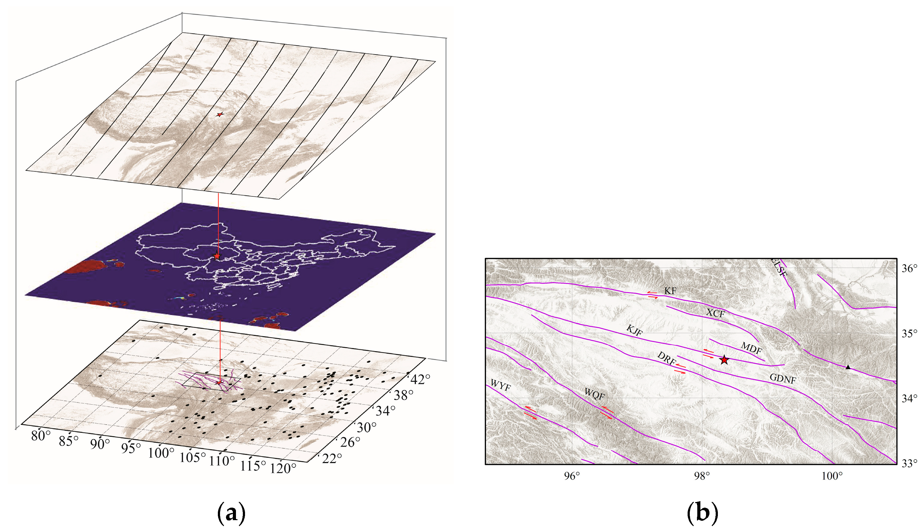
In recent years, the ground-based geomagnetic observation networks covering the entire Chinese mainland (Figure 1a, lower panel) and the launch of the China Seismo–Electromagnetic Satellite (CSES) in 2018 have provided us with the opportunity to further test these hypotheses. Most geomagnetic sites have favorable observation conditions and provide reliable data. CSES is the first space-based platform in China for earthquake observations and geophysical field measurements [37]. So far, CSES has successfully observed the response of in situ PAP O+ density and in situ LAP electron density to some seismic events [38].

On 22 May 2021, the Madoi 7.4 earthquake struck Qinghai Province in northwest China, with a longitude of 98.34° E, a latitude of 34.59° N, and a focal depth of 17 km. The epicenter was located at the Kunlun Pass–Jiancuo Fault, one of a series of nearly parallel active faults in the western Bayan Har block [39]. This fault is characterized by left–lateral slip. The Madoi earthquake was a strike–slip earthquake. And, it was also the first earthquake with a magnitude greater than 7.0 to hit the Chinese mainland since the launch of the CSES.

Over the past two years, scientists have conducted extensive research on the Madoi earthquake. Jing et al. [40] found anomalies in microwave brightness temperature and outgoing longwave radiation prior to the Madoi earthquake. Yang et al. [41] found thermal infrared brightness temperature anomalies before this event. Du and Zhang [42] investigated the anomalies of several parameters of the CSES satellite before the earthquake, including electron density, electron temperature, and ion compositions. Huang et al. [43] not only studied the data from multiple payloads of the CSES satellite but also analyzed the changes in total electron content (TEC) observed using GPS receivers before the Madoi earthquake. Li et al. [44] reported the earthquake risk near the epicenter based on the CSES data before the event.

Some of the current research focuses on analyzing satellite data, while others focus on analyzing ground-based data. However, the combination of these two is often limited to the joint analysis of satellite data and observations from a few individual ground-based sites. Data from the ground observation network is not being effectively utilized. We will utilize a novel approach to extract anomalies from geomagnetic network data and will investigate the abnormal changes from the ground to the ionosphere before the Madoi earthquake.

We will investigate the response of electromagnetic signals to the Madoi earthquake by combining ground-based geomagnetic data, outgoing long-wave radiation (OLR) detected by NOAA satellites, and ionospheric data from the CSES satellite. Figure 1a shows the stereoscopic data used in this work. This paper is organized as follows: In Section 2, we introduce the observational datasets, processing methods, and results. In Section 3, the results from various datasets will be analyzed synthetically, and the possible coupling mechanism of LAIC will be discussed. And, some brief conclusions will be given in Section 4.

2. Datasets and Processing

Previous studies [45,46] have reported that areas of stress accumulation in the Earth’s crust are often significantly larger than the fault rupture zones of earthquakes. According to Dobrovolsky’s research, there is a relationship between the radius of the earthquake preparation zone (R) and the magnitude of the earthquake (M), as follows: $\mathrm{R}={10}^{0.43\mathrm{M}}$. When the magnitude of an earthquake exceeds 7.0, the radius of the earthquake preparation zone extends beyond 1000 km [47,48]. This work focuses on the abnormal changes that occurred within a 1000 km radius of the epicenter of the Madoi earthquake.

2.1. Ground–Based Geomagnetic Datasets

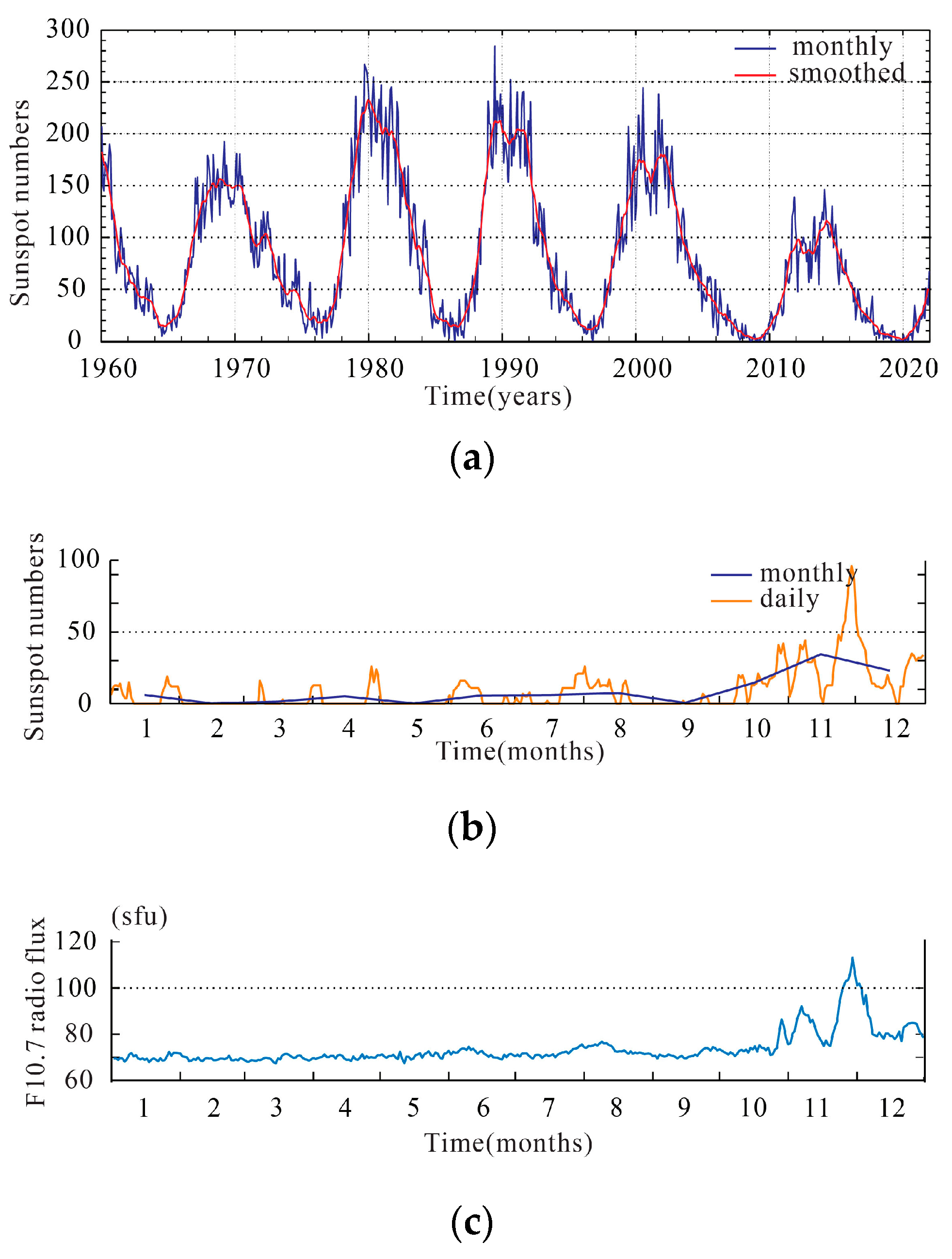
Strong earthquakes, severe magnetic storms, or solar activity can cause ionospheric perturbations, which could further affect the geomagnetic field [49]. Therefore, we made an effort to avoid these periods when selecting our data. As can be seen from Figure 2a, Solar Cycle 24 entered the solar minimum in 2018 and reached its lowest value in 2020. As can be seen from Figure 2b,c, the sunspot number remained below 40, and the F10.7 radio flux was less than 100 SFU (solar flux units), except for a few days from November 25 to 1 December 2020. This indicates that the solar activity had minimal impact on the ionosphere. No earthquakes with a magnitude greater than 7.0 occurred in Mainland China in 2020. To minimize the impact of magnetic storms and earthquakes, we selected data from 2020 as the reference.

It is well known that the observed fluctuations in the Z component of the geomagnetic field are usually smaller than those in other components during magnetic storm activity. Therefore, we utilized the Z component to study the response of the geomagnetic field to earthquakes.

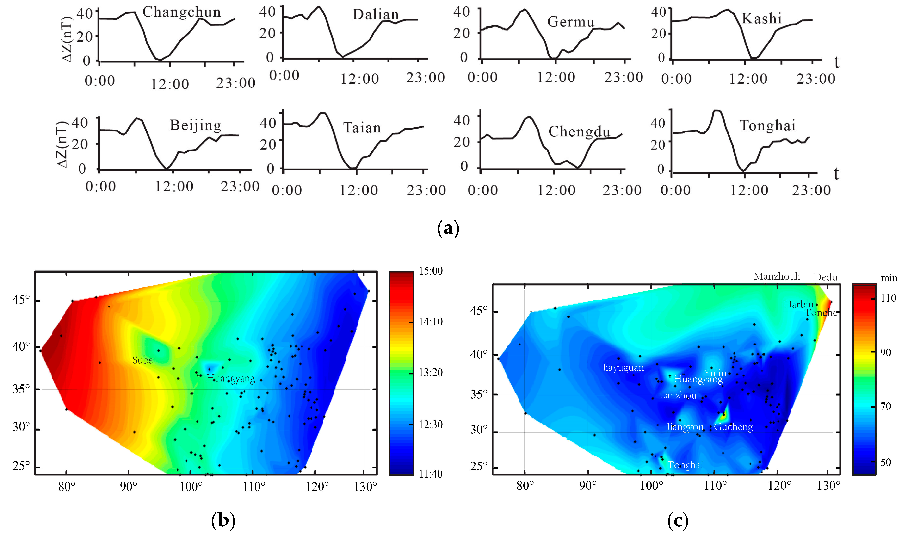
The regular diurnal variation in the geomagnetic field is a worldwide phenomenon [50]. Since the majority of the Chinese mainland is located in the mid-latitude of the northern hemisphere, the observed diurnal variation in the Z component closely resembles a cosine curve. In other words, the maximum occurs in the morning and evening, while the minimum occurs around noon (Figure 3a). The timing of the minimum occurrence is a key feature of the diurnal phase of the Z component. We will use it to describe the phase characteristics of the Z component. For simplicity, we will refer to it as the Low-Point-Time below. We will use the residuals of Low-Point-Time to demonstrate the disturbance of the geomagnetic field.

For a single station, the phase of the diurnal variation of geomagnetism does not change significantly from day to day. The Low-Point-Time of the geomagnetic Z component follows a normal distribution. Approximately 95% of the phasic deviations are less than two times the standard deviation. However, the diurnal phases of sites at different spatial locations vary greatly [51].

We calculate the average value and the standard deviation of the geomagnetic Z component Low-Point-Time observed at each station in 2020 using Formulas (1) and (2).

$$\overline{\mathrm{T}}=\frac{{\mathrm{t}}_1+{\mathrm{t}}_1+\dots +{\mathrm{t}}_{\mathrm{N}}}{\mathrm{N}}=\frac{{\sum }_{\mathrm{i}=1}^{\mathrm{N}}{\mathrm{t}}_{\mathrm{i}}}{\mathrm{N}}$$

(1)

$$\mathsf{\sigma }=\sqrt{\frac{{\sum }_{\mathrm{i}=1}^{\mathrm{N}}{({\mathrm{t}}_{\mathrm{i}}-\overline{\mathrm{T}})}^2}{\mathrm{N}}}$$

(2)

where ${\mathrm{t}}_{\mathrm{i}}$ is the Low-Point-Time of the $\mathrm{i}\mathrm{t}\mathrm{h}$ day and N is the number of days. $\overline{\mathrm{T}}$ is the average value of Low-Point-Time of each station. σ is the standard deviation of the Low-Point-Time. The average value of the Low-Point-Time shows significant longitude dependence (Figure 3b). That is to say, the Low-Point-Time is becoming later from east to west, except for a few stations (such as Huangyang and Subei), which are slightly lagging behind the surrounding area.

The standard deviation of the Low-Point-Time at most stations in the mid–latitude (i.e., from 30° N to 40° N) is less than 60 min. In addition, some stations have a slightly larger standard deviation. For example, the standard deviation of Gucheng is 89 min, which is significantly higher than that of the surrounding regions. The standard deviations of Huangyan Station, Yulin Station, Jiayuguan Station, Jiangyou Station, and Lanzhou Station are 72 min, 69 min, 69 min, 68 min, and 66 min, respectively, which are slightly higher than those of the surrounding areas. At high latitudes, the standard deviation is much larger. For example, the standard deviation of Tonghe Station is as high as 116 min, and the standard deviations of Dedu, Manzhouli, and Harbin are 86 min, 82 min, and 82 min. In general, geomagnetic disturbances are higher at high latitudes than in the mid–latitudes (Figure 3c), and the geomagnetic data are reliable.

We extract the portion where the standard deviation exceeds the threshold. Firstly, we use Formula (3) to calculate the difference between the observed value and the average value of the Low-Point-Time. Those with a difference of less than two standard deviations are considered within normal fluctuations. Then, Formula (4) is used to calculate the residuals that exceed two times the standard deviation observed at each station.

$$\Delta \mathrm{t}={\mathrm{t}}_{\mathrm{i}}-\overline{\mathrm{T}}$$

(3)

$$\Delta \Delta \mathrm{t}=\left\{\begin{array}{cc}\Delta \mathrm{t}-2\mathsf{\sigma }& (\Delta \mathrm{t}>2\mathsf{\sigma },\mathrm{o}\mathrm{r} \Delta \mathrm{t}<-2\mathsf{\sigma })\\ 0& (-2\mathsf{\sigma }\le \Delta \mathrm{t}\le 2\mathsf{\sigma })\end{array}\right.$$

(4)

where $\Delta \mathrm{t}$ is the part where the Low-Point-Time exceeds the standard deviation. $\Delta \Delta \mathrm{t}$ is a variable used to compare the residuals with two times the standard deviation.

We take two times the standard deviation as the threshold. To highlight the portion that exceeds the threshold value, we set the residuals to zero within the range of (−2σ, 2σ).

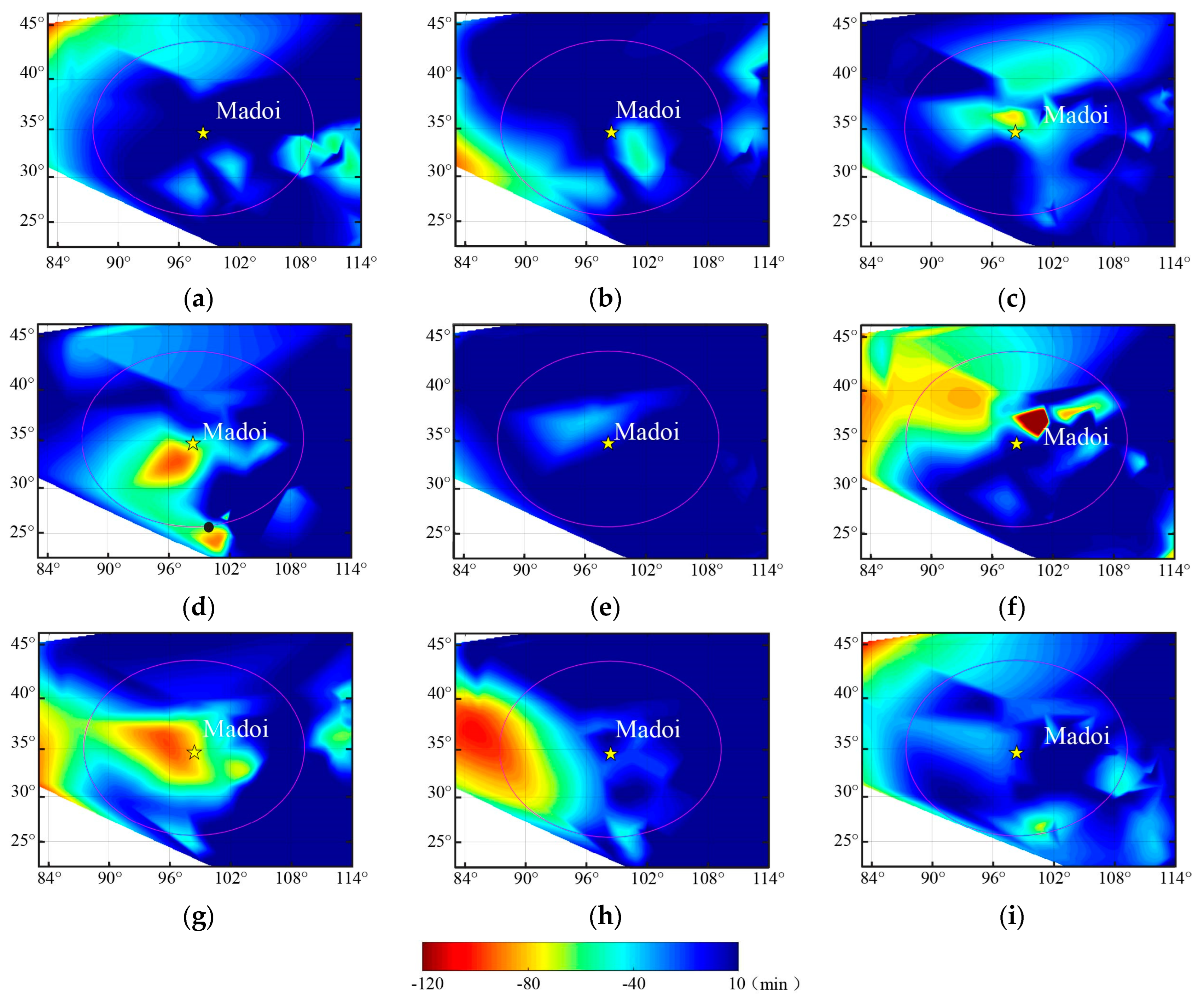
As shown in Figure 4, few residuals of Low-Point-Time near the epicenter exceed two times the standard deviation on 16 May 2021 (Figure 4a). On 17 May, the residuals southeast of the epicenter exceeded the threshold slightly. On 18 May, the residuals to the northwest and north of the epicenter exceeded the threshold. The range of high residuals was much greater than that on 17 May. On 20 May, the residual was surprisingly small. On 19 May, the residuals in the southeast of the epicenter exceeded the threshold. The region of high residual is divided into two parts. One is around (97.6° E, 34.2° N), and the other is near (101.6° E, 23.7° N). On 21 May, the residual in the north and northeast of the epicenter was more than 120 min. On 22 May, the day the Ms7.4 Madoi earthquake occurred, the area with residuals exceeding the threshold covered the entire epicenter (see Figure 4g). Later, on 23 May and 24, the residuals near the epicenter gradually decreased below the threshold. In summary, the residuals that exceeded the threshold were small in the first few days and then increased gradually day by day. Eventually, they disappeared after the earthquake.

2.2. Earth Radiation Observation

To investigate the presence of thermal anomalies around the epicenter of the Madoi earthquake, we analyzed the infrared emissions obtained from the OLR data collected by NOAA satellites.

We took the data from 15 May, which is the closest day to the study period, as a reference. Then, we subtracted the data on 15 May from each day of the study period. The differences indicate the variation in thermal infrared in different regions during those days.

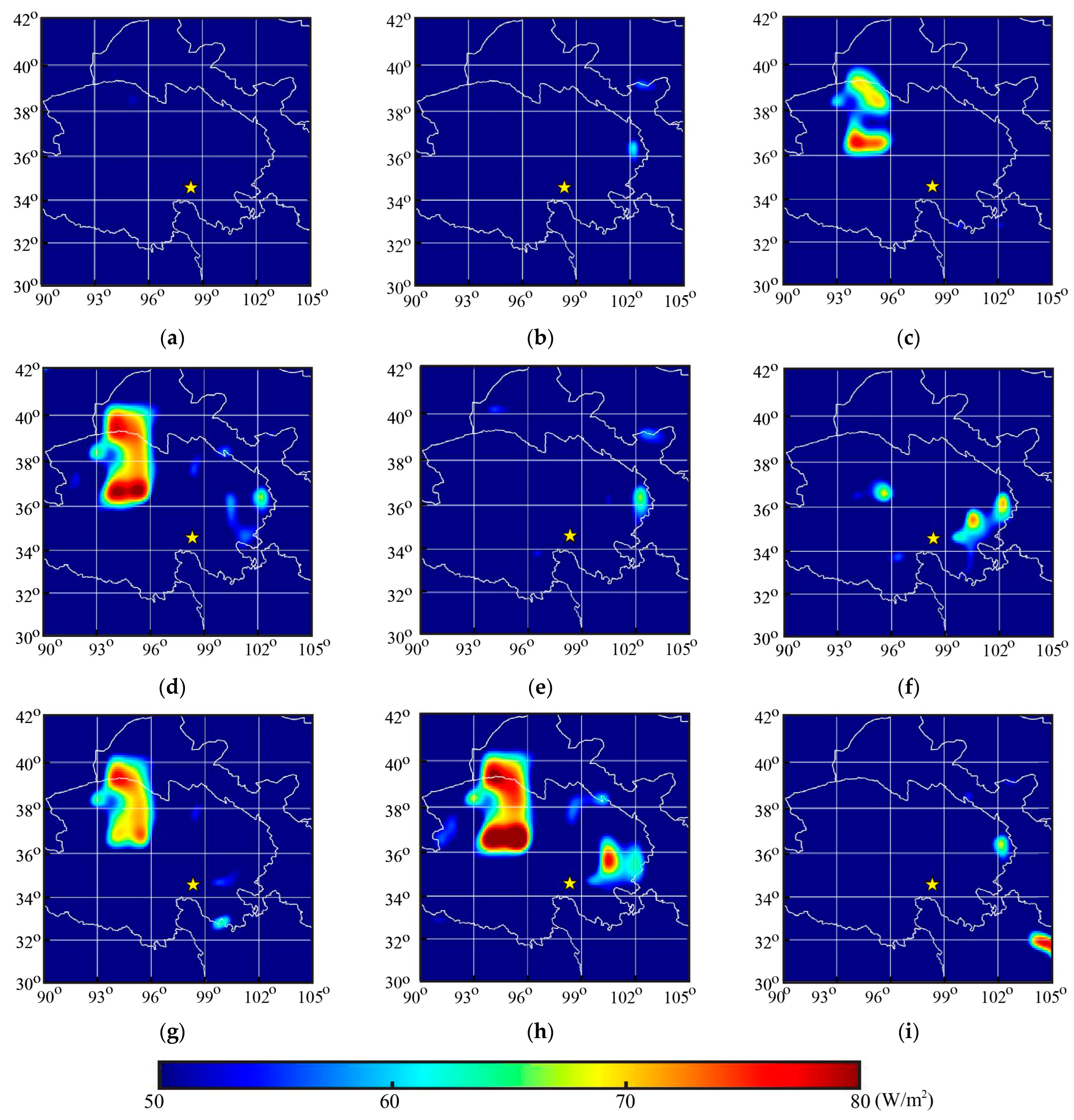
As shown in Figure 5, there was no significant increase in thermal infrared radiation in the study area on 16 May and 17 May compared with that on 15 May (see Figure 5a,b). On 18 May, the OLR radiation increased to the northwest of the epicenter, reaching a maximum amplitude of 74 W/m² (Figure 5c). There were also significant thermal anomalies in the same region on 19, 22, and 23 May (Figure 5d,g,h). On 19 May, the maximum increase in thermal warming reached 90 W/m². On 24 May, the warming phenomenon near the epicenter disappeared. During our study period, infrared anomalies appeared before the earthquake and disappeared on the third day after the earthquake. However, there were few anomalies on 20 and 21 May.

2.3. Ionospheric Data from the CSES

In this paper, we investigate the ionospheric response to the Madoi earthquake using LAP electron density and O+ density data from the night orbits. The ionosphere is the ionized part of the atmosphere that extends from about 50 to 1000 km above the Earth’s surface. Obara et al. [52] demonstrated an increase in electron flux at satellite altitude as a result of a geomagnetic storm, using an NOAA satellite.

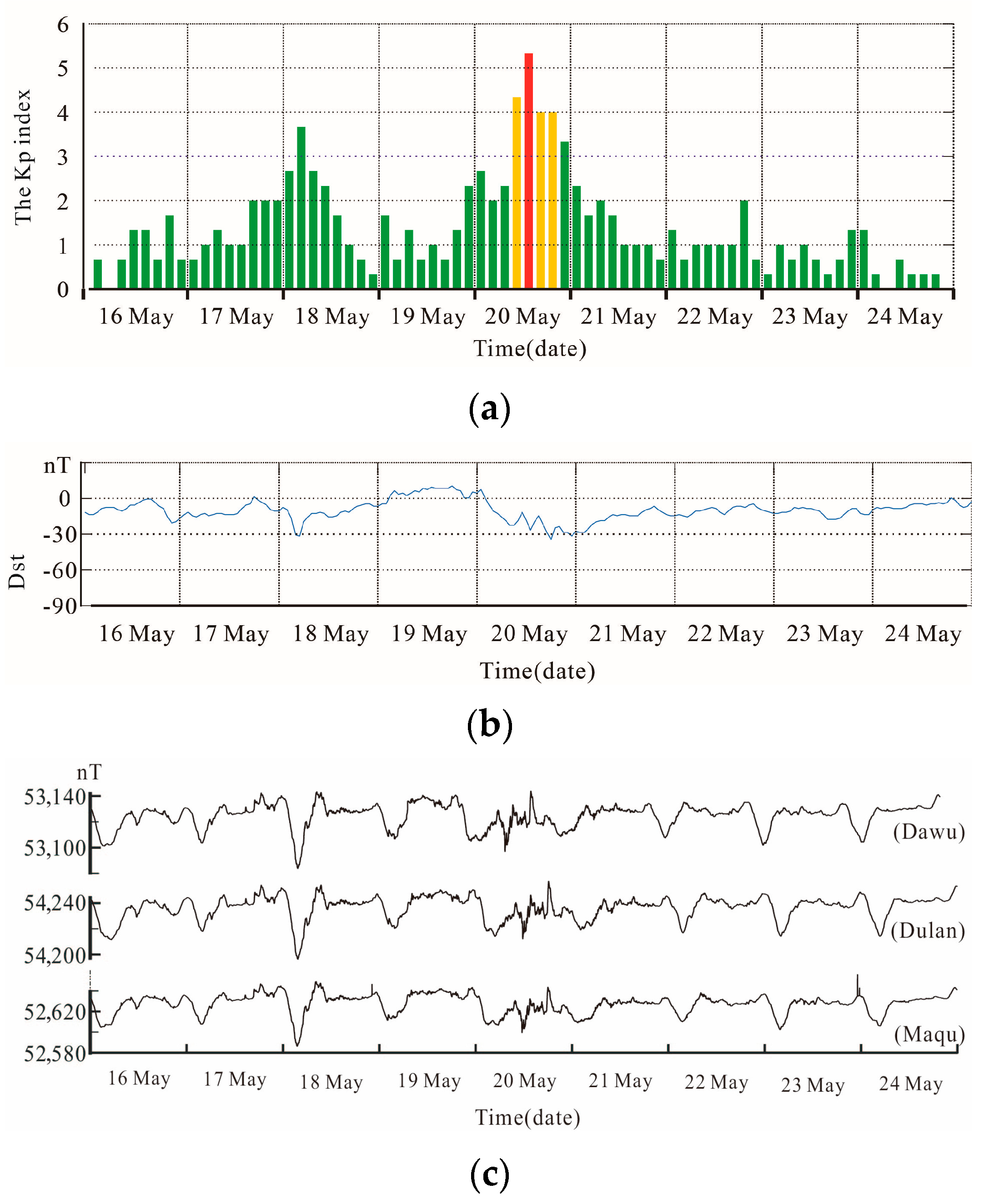
Generally, the interplanetary three–hour magnetic index, known as the Kp index, is used to describe global magnetic storms. Generally, geomagnetic activity is quiet when Kp is less than 3. However, the amplitude of the disturbance varies at different latitudes. The Dst index mainly reflects the influence of the ring current on the magnetic field, making it a better indicator and measurement of disturbances in low–latitude regions. To exclude the possible effect of external forces, data were selected only during periods of geomagnetic quiet time (|Dst| ≤ 30 nT and Kp ≤ 3). One can see from Figure 6 that there are parts of Kp indices larger than 3 and Dst < −30 on 18 and 20 May. Especially on 20 May, the Kp index reached a high of 5.33. It can also be observed from Figure 6c that the geomagnetic F component was affected by magnetic storm activity on 18 and 20 May.

The revisiting period of the CSES satellite was five days. We selected data from two revisiting periods before and after the Madoi earthquake. We excluded the data from 18 May and 20 May due to magnetic storms. Finally, we displayed all the data observed from different orbits during one revisiting period in the same image (Figure 7).

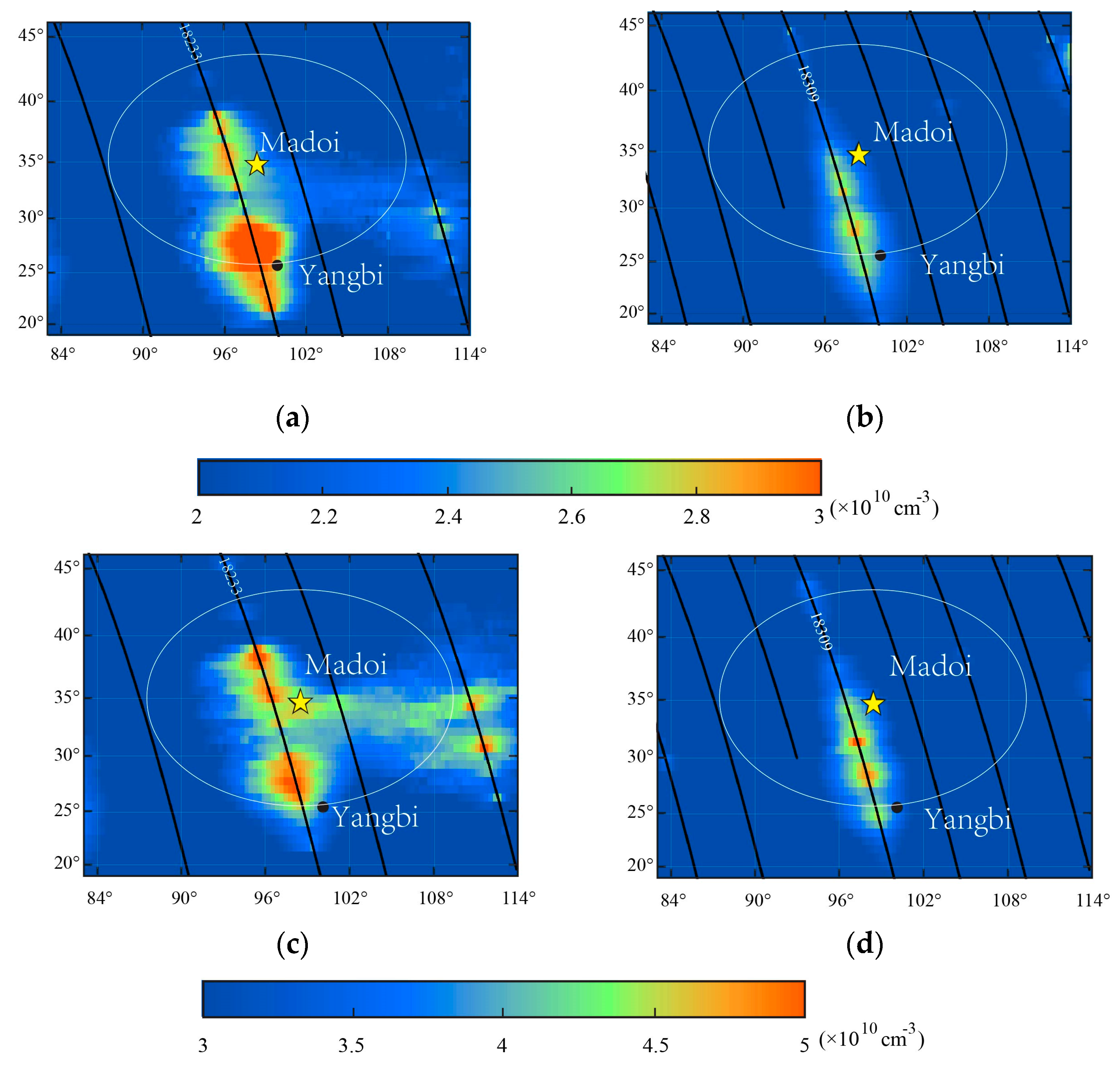
During the first revisiting period (from 16 May to 19 May), when the CSES satellite flew over the epicenter, orbit 18,233 recorded the ionospheric plasma disturbances detected by the PAP and LAP payloads, respectively (see Figure 7a,c). We can observe a significant increase in the density of O+ and electrons from the same orbit. The regions of plasma disturbance extended southeast from approximately 35° N to around 20° N. During the second revisiting period (from 21 May to 25 May), the electron density and O+ density detected from orbit 18,309 were still significantly higher over the epicenter compared with that of the other regions. Although the spatial range of high electron and O+ density was smaller than that observed in the previous revisiting period (see Figure 7b,d). The area of plasma density enhancement recorded during both revisiting periods had two focal points, particularly in the first revisiting period.

3. Result Analysis

This work presents a multi–parametric approach to investigate the pre–seismic anomaly during and before the Madoi earthquake that took place in China on 22 May, 2021. The ground-based data from the China Geomagnetic Networks, the OLR data from the NOAA satellite, and the plasma data from the CSES satellite were used in this work.

We proposed a method to extract geomagnetic anomalies using the Low-Point-Time residuals of the Z component of the geomagnetic field. The results show that the diurnal phasic variation in the Z component of the geomagnetic field near the epicenter changes significantly from 16 to 24 May, particularly on 19, 21, and 22 May. During this period, there was also an increase in atmospheric OLR radiation within the seismogenic zone. Although the high–radiation area is relatively farther from the epicenter, it still falls within Dobrovolsky’s radius. The anomalies in both the lithosphere and atmosphere reached a high magnitude on 18 May, 19 May, and 22 May. Previous studies have found that a similar phenomenon occurred before the Wenchuan earthquake on 12 May 2008. On 9 May 2008, synchronized anomalies were observed in multiple spheres, which may indicate an imminent earthquake.

In addition, during these two revisiting periods, orbit 18,233 and orbit 18,309 of the CSES satellite flew over the epicenter and recorded increases in electron density and O+ density. There are two regions with an increased plasma concentration (see Figure 7). The focal point of the northern region is located at (97.6° E, 34.2° N), near the epicenter of the Madoi earthquake. The southern focus is around (97.6° E, 34.2° N). An M = 6.4 Yangbi earthquake hit the southern area 4 h before the Madoi earthquake, which occurred at 21:48 on 21 May, Beijing Time. It is worth mentioning that the spatial distribution of geomagnetic phase residuals, extracted using our method, is remarkably consistent with plasma disturbances detected using the CSES satellite. On 19 May, there were also two similar focal points on the distribution plot of the residuals of Z component Low-Point-Time (Figure 4d). It is easy to imagine that the high–value region in the south is connected to the Yangbi earthquake. Since the subject of this study is the Madoi earthquake, we will not delve into the details of the southern focus. Although the data from each geosphere differs in temporal and spatial resolution, abnormal changes of varying degrees were observed in the lithosphere, atmosphere, and ionosphere before the Madoi earthquake.

Freund et al. [53] conducted laboratory experiments to compress rocks and to simulate tectonic plate shifts. The results showed that mobile positive holes (p–holes) can be activated in the crust due to microfractures during the dilatancy of earthquake preparation. The diffusion and outflow of these holes can further generate currents, radiations, electric fields, and magnetic fields on the Earth’s surface. Infrared emissions are expected to occur when p–hole recombine with electrons at the free surfaces [54,55]. Takeuchi et al. [56] proposed a detailed electrostatic channel model based on Freud’s p–holes theory and experimental results.

The P-holes are activated in a stressed fault zone and spread into the surrounding ground. Some of them reach the ground surface and form a positive surface potential over a large area around the epicenter. This potential creates an upward vertical electric field that penetrates the ionosphere through the atmosphere. The electrons “e⁻” in the ionosphere are forced downward and recombine with neutral particles “n” or positive ions “e⁺” in the atmosphere, which affects the density of electrons (or other plasma) in the ionosphere. Such an electric field can induce an abnormal magnetic field. The energy released by p-hole recombination is in the form of infrared emissions, which can potentially contribute to infrared warming. A detailed description can be found in reference [56].

In this work, almost all types of anomalies predicted using the electrostatic channel model were observed before or during the earthquake. So, there might be a coupling between the lithosphere, atmosphere, and ionosphere through electrostatic channels during the preparation and occurrence of the Madoi earthquake.

So far, no model can perfectly explain all the mechanisms of LAIC, and determining these mechanisms remains challenging. The study of seismic anomalies is still at the phenomenological level. Collecting more observations is important for further exploration of the lithosphere–atmosphere–ionosphere coupling mechanism associated with earthquakes.

However, there are still significant drawbacks in this study. The Earth’s ionosphere is a part of the atmosphere that extends from an altitude of about 50 km to over 1000 km. Because the altitude of the CSES satellite is about 500 km, it cannot record disturbances over the entire ionospheric height like GNSS–TEC can. Yue et al. [57] reported that significant TEC anomalies were observed three days before the earthquake. We have identified anomalies recorded on the two orbits that passed over the epicenter on 16 and 21 May. However, we cannot confirm if there are anomalies on the other days since the CSES satellite revisits every five days. Dong et al. [58] detected ionospheric perturbations in the conjugate regions using GPS TEC. We do not pay much attention to the magnetic conjugated regions of the Chinese mainland because of the distinct ionospheric backgrounds of the two opposite hemispheres.

In addition, the phenomena observed in this work are still somewhat different from what was expected. There are still many problems that cannot be explained in this work. For example, the distribution of plasma disturbances, thermal infrared warming, and high geomagnetic residuals does not strictly correspond in space. It might be related to spatial resolution, temporal resolution, and the laws governing the changing characteristics of the observed objects. It may not be possible to achieve complete consistency among the phenomena of different geospheres. In addition, there were almost no geomagnetic residuals that exceeded the threshold on 20 May during the study period. Furthermore, the increments in OLR on 20 and 21 May were very small. It is difficult to explain the factors that cause them to decrease during this period.

The Madoi earthquake in 2021 is the largest earthquake in mainland China since the launch of the CSES satellite. This work exemplifies the integrated use of the geomagnetic network and the CSES data, providing additional evidence for future LAIC research.

4. Conclusions

In this paper, we investigated the anomalies within Dobrovolksy’s radius before and during the Madoi earthquake. We are utilizing a novel approach to identify anomalies in the geomagnetic field. The following phenomena that we summarize are helpful for further research on earthquake–related LAIC. However, there are still some unexplained problems.

• Dobrovolksy’s radius has revealed abnormal changes in the lithosphere, atmosphere, and ionosphere.
• Despite the differences in spatial and temporal resolutions, some temporal similarities have been found between geomagnetic diurnal phase anomalies in the lithosphere and enhancements in atmospheric OLR.
• There are two regions of high value for both the ground–based geomagnetic high residual and the ionospheric disturbances observed with CSES. The northern one is near the epicenter of the Madoi earthquake, and the southern one is near the epicenter of the Yangbi earthquake, which occurred 4 h before the Madoi earthquake.
• In this study, we observed almost all of the physical phenomena that may occur during earthquake preparation, as predicted using the electrostatic channel model. The electrostatic channel model can explain the changes observed in the Madoi earthquake very well. So, we inferred that the electrostatic channel might be the possible mechanism for coupling between the lithosphere, atmosphere, and ionosphere during the Madoi earthquake.

References

- Fraser-Smith, A.C.; Bernardi, A.; Mcgill, P.R.; Ladd, M.E.; Helliwell, R.A.; Villard, O.G., Jr. Low-frequency magnetic field measurements near the epicenter of the Ms7.1 Loma Prieta earthquake. Geophys. Res. Lett. 1990, 17, 1465–1468. [Google Scholar] [CrossRef]
- Kopytenko, Y.A. Ultra Low Frequency Emission Associated with Spitak Earthquake and Following Aftershock Activity Using Geomagnetic Pulsation Data at Observatories Dusheti and Vardziya; IZMIRAN: Moscow, Russia, 1990. [Google Scholar]
- Molchanov, O.A.; Kopytenko, Y.A.; Voronov, P.M.; Kopytenko, E.A.; Matiashvili, T.G.; Fraser-Smith, A.C.; Bernardi, A. Results of ulf magnetic field measurements near the epicenters of the Spitak (ms=6.9) and Loma Prieta (ms=7.1) earthquakes: Comparative analysis. Geophys. Res. Lett. 1992, 19, 1495–1498. [Google Scholar] [CrossRef]
- Prattes, G.; Schwingenschuh, K.; Eichelberger, H.U.; Magnes, W.; Boudjada, M.; Stachel, M.; Vellante, M.; Villante, U.; Wesztergom, V.; Nenovski, P. Ultra Low Frequency (ULF) European multi station magnetic field analysis before and during the 2009 earthquak eat L’Aquila regarding regional geotechnical information. Nat. Hazards Earth Syst. Sci. 2011, 11, 1959–1968. [Google Scholar] [CrossRef]
- Rolland, L.M.; Lognonné, P.; Astafyeva, E.; Kherani, E.A.; Kobayashi, N.; Mann, M.; Munekane, H. The resonant response of the ionosphere imaged after the 2011 off the Pacific coast of Tohoku Earthquake. Earth Planets Space 2011, 63, 853–857. [Google Scholar] [CrossRef]
- Liu, J.; Wan, W.X.; Huang, J.P.; Zhang, X.M.; Zhao, S.F.; Ouyang, X.Y.; Zeren, Z.M. Electron density perturbation before Chile M8.8 earthquake. Chin. J. Geophys. 2011, 54, 271–2725. (In Chinese) [Google Scholar]
- Zhang, X.M.; Qian, J.D.; Ouyang, X.Y.; Shen, X.H.; Cai, J.A.; Zhao, S.F. Ionospheric electro magnetic disturbances observed on DEMETER satellite before an earthquake of M7.9 in Chile. Prog. Geophys. 2009, 24, 1196–1203. (In Chinese) [Google Scholar]
- Stangl, G.; Boudjada, M.Y.; Biagi, P.F.; Krauss, S.; Maier, A.; Schwingenschuh, K.; Al-Haddad, E.; Parrot, M.; Voller, W. Investigation of TEC and VLF space measurements associated to L’aquila (Italy) earthquakes. Nat. Hazards Earth Syst. Sci. 2011, 11, 1019–1024. [Google Scholar] [CrossRef]
- Li, M.; Lu, J.; Parrot, M.; Tan, H.; Chang, Y.; Zhang, X.; Wang, Y. Review of unprecedented ULF electromagnetic anomalous emissions possibly related to the Wenchuan Ms=8.0 earthquake, on 12 May 2008. Nat. Hazards Earth Syst. Sci. 2013, 13, 279–286. [Google Scholar] [CrossRef]
- Zeng, Z.C.; Zhang, B.; Fang, G.Y.; Wang, D.F.; Yin, H.J. The analysis of ionospheric vaiations before Wenchuan earthquake with DEMETER data. Chin. J. Geophys. 2009, 52, 11–19. (In Chinese) [Google Scholar] [CrossRef]
- Zhang, X.; Shen, X.; Liu, J.; Ouyang, X.Y.; Qian, J.D.; Zhao, S.F. Analysis of ionospheric plasma perturbations before Wenchuan earthquake. Nat. Hazards Earth Syst. Sci. Discuss. 2009, 9, 1259–1266. [Google Scholar] [CrossRef]
- Qiang, Z.J.; Xu, X.D.; Dian, C.G. Thermal infrared anomaly precursor of impending earthquakes. Chin. Sci. 1991, 36, 319–323. [Google Scholar] [CrossRef]
- Aliano, C.; Corrado, R.; Filizzola, C.; Genzano, N.; Pergola, N.; Tramutoli, V. Robust TIR satellite techniques for monitoring earthquake active regions: Limits, mainachievements and perspectives. Ann. Geophys. 2008, 51, 303–318. [Google Scholar] [CrossRef]
- Tronin, A.A. Satellite thermal survey-a new tool for the study of seismoactive regions. Int. J. Remote Sens. 1996, 41, 1439–1455. [Google Scholar] [CrossRef]
- Tramutoli, V.; Bello, G.D.; Pergola, N.; Piscitelli, S. Robust satellite techniques for remote sensing of seismically active areas. Ann. Geofis. 2001, 44, 295–312. [Google Scholar] [CrossRef]
- Piroddi, L.; Ranieri, G.; Freund, F.; Trogu, A. Geology, tectonics and topography underlined by L’Aquila earthquake TIR precursors. Geophys. J. Int. 2014, 197, 1532–1536. [Google Scholar] [CrossRef]
- Saraf, A.K.; Choudhury, S. Satellite detects surface thermal anomalies associated with the Algerian earthquakes of May 2003. Int. J. Remote Sens. 2005, 26, 2705–2713. [Google Scholar] [CrossRef]
- Ouzounov, D.; Freund, F.T. Mid-infrared emission prior to strong earthquakes analyzed remote sensing data. Adv. Inspace Res. 2004, 33, 268–273. [Google Scholar] [CrossRef]
- Ouzounov, D.; Liu, D.F.; Kang, C.L.; Cervone, G.; Kafatos, M.; Taylor, P. The outgoing long-wave radiation variability prior to the major earthquake by analyzing IR satellite data. Tectonophysics 2007, 421, 211–220. [Google Scholar] [CrossRef]
- Blackett, M.; Wooster, M.J.; Malamud, B.D. Exploring land surface temperature earthquake precursors: A focus on the Gujarat (India) earthquake of 2001. Geophys. Res. Lett. 2011, 38, L15303. [Google Scholar] [CrossRef]
- Namgaladze, A.A.; Klimenko, M.V.; Klimenko, V.V.; Zakharenkova, I.E. Physical mechanism and mathematical modeling of earthquake ionospheric precursors registered in total electron content. Geomagn. Aeron. 2009, 49, 252–262. [Google Scholar] [CrossRef]
- Klimenko, M.V.; Klimenko, V.V.; Zakharenkova, I.E.; Pulinets, S.A. Variations of equatorial electrojet as possible seismo-ionospheric precursor at the occurrence of TEC anomalies before strong earthquake. Adv. Space Res. 2012, 49, 509–517. [Google Scholar] [CrossRef]
- Artru, J.; Lognonné, P.; Blanc, E. Normal modes modelling of post-seismic ionospheric oscillations. Geophys. Res. Lett. 2001, 28, 697–700. [Google Scholar] [CrossRef]
- Hayakawa, M.; Molchanov, O.A.; NASDA/UEC Team. Summary report of NASDA’s earthquake remote sensing frontier project. Phys. Chem. Earth 2004, 29, 617–625. [Google Scholar] [CrossRef]
- Hayakawa, M.; Schekotov, A.; Izutsu, J.; Nickolaenko, A.P. Seismogenic effects in ULF/ELF/VLF electro magnetic waves. Int. J. Electron. Appl. Res. 2019, 6, 1–86. [Google Scholar]
- Sorokin, V.M.; Chmyrev, V.M.; Yaschenko, A.K. Electrodynamic model of the lower atmosphere and the ionosphere coupling. J. Atmos. Sol. Terr. Phys. 2001, 63, 1681–1691. [Google Scholar] [CrossRef]
- Rapoport, Y.; Grimalsky, V.; Hayakawa, M.; Ivchenko, V.; Juarez-R, D.; Koshevaya, S.; Gotynyan, O. Change of ionospheric plasma parameters under the influence of electric field which has lithospheric origin and due to radon emanation. Phys. Chem. Earth 2004, 29, 579–587. [Google Scholar] [CrossRef]
- Shalimov, S.; Gokhberg, M. Lithosphere-ionosphere coupling mechanism and its application to the earthquake in Iran on June 20, 1990. A review of ionospheric measurements and basic assumptions. Phys. Earth Planet. Inter. 1998, 105, 211–218. [Google Scholar] [CrossRef]
- Singh, B.; Kushwah, V.; Singh, O.P.; Lakshmi, D.R.; Reddy, B.M. Ionospheric perturbations caused by some major earthquakes in India. Phys. Chem. 2004, 29, 537–550. [Google Scholar] [CrossRef]
- Molchanov, O.A.; Hayakawa, M.; Rafalsky, V.A. Penetration characteristics of electromagnetic emissions from an underground seismic source into the atmosphere, ionosphere, and magnetosphere. J. Geophys. Res. 1995, 100, 1691–1712. [Google Scholar] [CrossRef]
- Grimalsky, V.V.; Kremenetsky, I.A.; Rapoport, Y.G. Excitation of electromagnetic waves in the lithosphere and their penetration into ionosphere and magetsphere. J. Atmos. Electr. 1999, 19, 101–117. [Google Scholar]
- Ghosh, S.; Chowdhury, S.; Kundu, S.; Sasmal, S.; Politis, D.Z.; Potirakis, S.M.; Hayakawa, M.; Chakraborty, S.; Chakrabarti, S.K. Unusual Surface Latent Heat Flux Variations and Their Critical Dynamics Revealed before Strong Earthquakes. Entropy 2022, 24, 23. [Google Scholar] [CrossRef]
- Freund, F.T. Stress-activated positive hole charge carriers in rocks and the generation of pre-earthquake signals. Electromagn. Phenom. Assoc. Earthq. 2009, 3, 41–96. [Google Scholar]
- Parrot, M.; Benoist, D.; Berthelier, J.J.; Błęcki, J.; Chapuis, Y.; Colin, F.; Elie, F.; Fergeau, P.; Lagoutte, D.; Lefeuvre, F. The magnetic field experiment IMSC and its data processing onboard DEMETER: Scientific objectives, description and first results. Planet. Space Sci. 2006, 54, 441–455. [Google Scholar] [CrossRef]
- Kuo, C.L.; Huba, J.D.; Joyce, G.; Lee, L.C. Ionosphere plasma bubbles and density variations induced by pre-earthquake rock currents and associated surface charges. J. Geophys. Res. 2011, 116, A10317. [Google Scholar] [CrossRef]
- Ouzounov, D.; Pulinets, S.; Hattori, K.; Taylor, P. Pre-Earthquake Processes: A Multidisciplinary Approach to Earthquake Prediction Studies; AGU Geophysical Monograph 234; Wiley: Hoboken, NJ, USA, 2018; 365p. [Google Scholar]
- Shen, X.H.; Zhang, X.M.; Yuan, S.G.; Wang, L.W.; Gao, J.B.; Huang, J.P.; Zhu, X.H.; Piergiorgio, P.; Dai, J.P. The state-of-the-art of the China Seismo-Electromagnetic Satellite mission. Sci. China Technol. Sci. 2018, 61, 634–642. [Google Scholar] [CrossRef]
- Li, M.; Shen, X.H.; Parrot, M.; Zhang, X.M.; Zhang, Y.; Yu, C.; Yan, R.; Liu, D.P.; Lu, H.X.; Guo, F. Primary joint statistical seismic influence on iIonospheric parameters recorded by the CSES and DEMETER satellites. J. Geophys. Res. Space Phys. 2020, 125, e2020JA028116. [Google Scholar] [CrossRef]
- Chen, G.H.; Li, Z.W.; Xu, X.W.; Sun, H.Y.; Ha, G.H.; Guo, P.; Su, P.; Yuan, Z.D.; Li, T. Co-seismic surface deformation and late Quaternary accumulated displacement along the seismogenic fault of the 2021 Madoi M7.4 earthquake and their implications for regional tectonics. Chin. J. Geophys. 2022, 65, 2984–3005. [Google Scholar]
- Jing, F.; Zhang, L.; Singh, R. Pronounced changes in thermal signals associated with the Madoi (China) M7.3 earthquake from passive microwave and infrared satellite data. Remote Sens. 2022, 14, 2539. [Google Scholar] [CrossRef]
- Yang, X.; Zhang, T.B.; Lu, Q.; Long, F.; Liang, M.J.; Wu, W.W.; Gong, Y.; Wei, J.X.; Wu, J. variation of thermal infrared brightness temperature anomalies in the Madoi earthquake and associated earthquakes in the Qinghai-Tibetan plateau (China). Front. Earth Sci. 2022, 10, 823540. [Google Scholar] [CrossRef]
- Du, X.; Zhang, X. Ionospheric Disturbances Possibly Associated with Yangbi Ms6.4 and Maduo Ms7.4 Earthquakes in China from China Seismo Electromagnetic Satellite. Atmosphere 2022, 13, 438. [Google Scholar] [CrossRef]
- Huang, J.P.; Wang, Q.; Yan, R.; Lin, J.; Zhao, S.F.; Chu, W.; Shen, X.H.; Zeren, Z.M.; Yang, Y.Y.; Cui, J.; et al. Pre-seismic multi-parameters variations before Yangbi and Madoi earthquakes on May 21, 2021. Nat. Hazards Res. 2023, 3, 27–34. [Google Scholar] [CrossRef]
- Li, M.; Wang, H.; Liu, J.; Shen, X. Two Large Earthquakes Registered by the CSES Satellite during Its Earthquake Prediction Practice in China. Atmosphere 2022, 13, 751. [Google Scholar] [CrossRef]
- Bedford, J.R.; Moreno, M.; Deng, Z.G.; Oncken, O.; Schurr, B.; John, T.; Báez, J.C.; Bevis, M. Months-long thousand-kilometre-scale wobbling before great subduction earthquakes. Nature 2020, 580, 628–635. [Google Scholar] [CrossRef] [PubMed]
- Chen, C.H.; Yeh, T.K.; Wen, S.; Meng, G.J.; Han, P.; Tang, C.C.; Liu, J.Y.; Wang, C.H. Unique Pre-Earthquake Deformation Patterns in the Spatial Domains from GPS in Taiwan. Remote Sens. 2020, 12, 366–385. [Google Scholar] [CrossRef]
- Dobrovolsky, I.P.; Zubkov, S.I.; Miachkin, V.I. Estimation of the size of earthquake preparation zones. Pure Appl. Geophys. 1979, 117, 1025–1044. [Google Scholar] [CrossRef]
- Chen, T.; Zhang, X.X.; Zhang, X.M.; Jin, X.B.; Wu, H.; Ti, S.; Li, R.K.; Li, L.; Wang, S.H. Imminent estimation of earthquake hazard by regional network monitoring the near surface vertical atmospheric electrostatic field. Chin. J. Geophys. 2021, 64, 1145–1154. (In Chinese) [Google Scholar]
- Ryu, K.; Lee, E.; Chae, J.S.; Parrot, M.; Pulinets, S. Seismo-ionospheric coupling appearing as equatorial electron density enhancements observed via DEMETER electron density measurements. J. Geophys. Res. Space Phys. 2014, 119, 8524–8542. [Google Scholar] [CrossRef]
- Chapman, S. The solar and lunar diurnal variations of terrestrial magnetism. Philos. Trans. R. Soc. Lond. 1919, 218, 1–118. [Google Scholar]
- Wang, Y.L.; Wu, Y.Y.; Lu, J.; Yu, S.R.; Li, M.X. Spatial distribution characteristics of geomagnetic Z component phase variation in Chinese mainland. Chin. J. Geophys. 2009, 52, 1033–1040. (In Chinese) [Google Scholar] [CrossRef]
- Obara, T.; Miyoshi, Y.; Morioka, A. Large enhancement of the outer belt electrons during magnetic storms. Earth Planet Space 2001, 53, 1163–1170. [Google Scholar] [CrossRef]
- Freud, F. Time-resolved study of charge generation and propagation in igneous rocks. J. Geophys. Res. 2000, 105, 11001–11019. [Google Scholar] [CrossRef]
- Freund, F.; Ouillon, G.; Scoville, J.; Sornette, D. Earthquake precursors in the light of peroxy defects theory: Critical review of systematic observations. Eur. Phys. J. Spec. Top. 2021, 230, 7–46. [Google Scholar] [CrossRef]
- Ouzounov, D.; Pulinets, S.; Parrot, M.; Hattori, K.; Taylor, P. Surveying the natural hazards by joint satellite and ground based analysis of Earth’s electromagnetic environment. In Proceedings of the EMSEV-DEMETER Joint Workshop, International Union of Geodesy and Geophysics, Sinaia, Romania, 7–12 September 2008. [Google Scholar]
- Takeuchi, A.; Lau, B.; Freund, F. Current and surface potential induced by stress-activated positive holes in igneous rocks. Phys. Chem. Earth 2006, 31, 240–247. [Google Scholar] [CrossRef]
- Yue, Y.; Koivula, H.; Bilker-Koivula, M.; Chen, Y.; Chen, F.; Chen, G. TEC Anomalies Detection for Qinghai and Yunnan Earthquakes on 21 May 2021. Remote Sens. 2022, 14, 4152. [Google Scholar] [CrossRef]
- Dong, L.; Zhang, X.; Du, X. Analysis of Ionospheric Perturbations Possibly Related to Yangbi Ms6.4 and Maduo Ms7.4 Earthquakes on 21 May 2021 in China Using GPS TEC and GIM TEC Data. Atmosphere 2022, 13, 1725. [Google Scholar] [CrossRef]
Figure 1.
Schematic presentation of the epicenter, active faults, and stereo monitoring of the Madoi earthquake: (upper panel of (a)) the orbits of the CSES; (middle panel of sub-figure (a)) OLR detected by NOAA satellite; (lower panel of (a)) black dots represent ground geomagnetic observations; (b) active faults in the western Bayan Har block; DRF: Dari fault; ELSF: Elashan fault; GDNF: Gandenan fault; KF: Kunlun fault; KJF: Kunlun Pass-Jiancuo fault; MDF: Madoi fault; TTHF: Tongtianhe fault; WQF:Wudaoliang-Qumalai fault; WYF: Wulan-Yushu fault;XCF: Xizangdagou-Changmahe fault (fault data comes from reference [39]), and the red star represent the epicenter of the Madoi earthquake.
Figure 2.
(a) Monthly and 13–month smoothed sunspot numbers over the last 6 cycles; (b) daily and monthly sunspot numbers in 2020. (Source: WDC–SILSO, Royal Observatory of Belgium, Brussels.) (c) The F10.7 radio flux during 2020.
Figure 3.
(a) Diurnal variation curves of the Z component of several Chinese geomagnetic stations; (b) the average value and the standard deviation of the geomagnetic Z component Low-Point-Time over mainland China in 2020, which shows very significant longitude dependence; (c) the standard deviation of the geomagnetic Z component Low-Point-Time over mainland China in 2020. The standard deviation in the north is higher than that in the south.
Figure 4.
Spatio—temporal evolution of Low-Point-Time residuals of geomagnetic Z component diurnal variation in the days before and after the Madoi Ms7.4 earthquake in Qinghai on 22 May, 2021. Sub–figures (a–i) represent the residuals from 16 May to 24 May, respectively. The circle presents Dobrovolsky’s radius, and the black dot in sub-figure (d) represents the epicenter of the Yangbi earthquake.
Figure 5.
The OLR was observed by NOAA satellites near the epicenter of the Madoi earthquake. Sub-figures (a–i) show the increase in OLR emissions from 16 May to 24 May compared with that on 15 May. Therein, the amplitude of OLR reached 74 W/m2 on 18 May (c) and 90W/m2 on 23 May (h).
Figure 6.
Dst and Kp indices from 6 May to 24 May. (a) One of the Kp indices was >3 on 18 May. On 20 May, there were three Kp indices >3, one of which was 5.33. (b) The Dst of the corresponding period is close to −30 nT. (c) The geomagnetic F component of three observatories (i.e., Dawu, Dulan, and Maqu) were slightly disturbed by magnetic storm activity on 18 and 20 May.
Figure 7.
The spatial variation in LAP electron density and O+ density was observed via the CSES satellite during two revisit periods before and after the Madoi earthquake. One of the revisiting periods ran from 16 May to 20 May, and the other ran from 21 May to 25 May. Black arcs represent the orbits of the CSES satellite. The yellow star represents the epicenter of the Madoi earthquake, while the black dot represents the epicenter of the Yangbi earthquake, which occurred four hours prior to the Madoi earthquake. (a) LAP electron density from 16 May to 20 May 2021; (b) LAP electron density from 21 May to 25 May 2021; (c) PAP O+ density from 16 May to 20 May; (d) PAP O+ density from 21 May to 25 May. Thereinto, the data on 18 and 20 May were not used due to the geomagnetic storms.
Disclaimer/Publisher’s Note: The statements, opinions and data contained in all publications are solely those of the individual author(s) and contributor(s) and not of MDPI and/or the editor(s). MDPI and/or the editor(s) disclaim responsibility for any injury to people or property resulting from any ideas, methods, instructions or products referred to in the content. |
© 2023 by the authors. Licensee MDPI, Basel, Switzerland. This article is an open access article distributed under the terms and conditions of the Creative Commons Attribution (CC BY) license (https://creativecommons.org/licenses/by/4.0/).
Share and Cite
MDPI and ACS Style
Wang, Y.; Ma, W.; Zhao, B.; Yue, C.; Zhu, P.; Yu, C.; Yao, L. Responses to the Preparation of the 2021 M7.4 Madoi Earthquake in the Lithosphere–Atmosphere–Ionosphere System. Atmosphere 2023, 14, 1315. https://doi.org/10.3390/atmos14081315
AMA Style
Wang Y, Ma W, Zhao B, Yue C, Zhu P, Yu C, Yao L. Responses to the Preparation of the 2021 M7.4 Madoi Earthquake in the Lithosphere–Atmosphere–Ionosphere System. Atmosphere. 2023; 14(8):1315. https://doi.org/10.3390/atmos14081315
Chicago/Turabian StyleWang, Yali, Weiyu Ma, Binbin Zhao, Chong Yue, Peiyu Zhu, Chen Yu, and Li Yao. 2023. "Responses to the Preparation of the 2021 M7.4 Madoi Earthquake in the Lithosphere–Atmosphere–Ionosphere System" Atmosphere 14, no. 8: 1315. https://doi.org/10.3390/atmos14081315
Note that from the first issue of 2016, this journal uses article numbers instead of page numbers. See further details here.