
Evaluation of WRF Performance in Simulating an Extreme Precipitation Event over the South of Minas Gerais, Brazil
Institute of Natural Resources, Federal University of Itajubá, Itajubá 37500-903, Brazil
*
Author to whom correspondence should be addressed.
Atmosphere 2023, 14(8), 1276; https://doi.org/10.3390/atmos14081276
Submission received: 28 June 2023
/
Revised: 1 August 2023
/
Accepted: 10 August 2023
/
Published: 12 August 2023
(This article belongs to the Special Issue Extreme Hydrometeorological Forecasting)
Abstract
:Extreme precipitation events are becoming increasingly frequent and intense in southeastern Brazil, leading to socio-economic problems. While it is not possible to control these events, providing accurate weather forecasts can help society be better prepared. In this study, we assess the performance of the Weather Research and Forecasting (WRF) model in simulating a period of extreme precipitation from 31 December 2021 to 2 January 2022 in the southern region of Minas Gerais (SMG) state in southeastern Brazil. We conducted five simulations using two nested grids: a 12 km grid (coarse resolution) and a 3 km grid (high resolution). For the coarse resolution, we tested the performance of five cumulus convection parameterization schemes: Kain–Fritsch, Betts–Miller–Janjic, Grell–Freitas, Grell–Devenyi, and New Tiedke. We evaluated the impact of these simulations on driving the high-resolution simulations. To assess the performance of the simulations, we compared them with satellite estimates, in situ precipitation measurements from thirteen meteorological stations, and other variables from ERA5 reanalysis. Based on the results, we found that the Grell–Freitas scheme has better performance in simulating the spatial pattern and intensity of precipitation for the studied region when compared with the other four analyzed schemes.
1. Introduction
Extreme precipitation events responsible for severe economic impacts and loss of lives have been a cause of concern in Brazil for several decades [1,2,3,4,5]. However, the observed positive trends of the seasonal amount and daily extremes of rainfall reported by studies such as [6,7,8,9], and the dramatic consequences of recent extreme events in cities of Rio de Janeiro [1] (2022) and São Paulo [10] (2023) states in the Southeastern Region of Brazil (SEB), have caused more concern and brought the attention of decision-makers and the general public to the weather forecast, as many of these cases were not adequately predicted by numerical models.
During the austral rainy season of 2021/2022, the SEB, where more than 87 million people live—approximately 42.04% of the total Brazilian population [11]—registered several daily extreme events of rainfall [1,5,12]. One of the most critical events occurred in Petrópolis, a historical city in the Mountains of Rio de Janeiro State (RJ). In three hours on February 15th of 2022, 252.8 mm of rain caused landslides and flooding that resulted in billions in economic losses and 233 deaths [1,13]. This value is more than expected for the whole month of February [14] (a climatological average of 238.2 mm). One month later, on March 20th of 2022, Petrópolis was affected by another extreme event when 358.6 mm of rain was registered in 24 h [12]. The amount of precipitation in 24 h was higher in March, but in terms of casualties and social-economic impacts February’s event was the worst. Other significant events were reported in different cities of the SEB, such as Brumadinho (206.56 mm in 24 horas on 8 January 2022) and Muriaé (95.21 mm in 11 h on 9 January 2022) in Minas Gerais (MG) state [12].
In the SEB, the south of Minas Gerais (SMG) is affected by high volumes of precipitation with severe social-economic impacts, especially during the austral summer. The region has a monsoon climate with two well-defined seasons: the dry season between April and September and the rainy season from October to March [8,15]. Between December 31st of 2021 and January 2nd of 2022, for instance, extreme precipitation values were recorded in the area near the Mantiqueira Mountains (Serra da Mantiqueira) close to the border between the states of MG and São Paulo (SP). As a result, one of the main highways connecting the two states was blocked due to the collapse of barriers and tree falls, which caused inconvenience to the population and losses to the local economy [16].
In addition, the level of the Sapucai River, which crosses the Itajuba Municipality, reached the attention level at 842.98 m on January 01 of 2022 (meteorologia.unifei.edu.br/hidrologia).
For the SMG, numerical forecasts with the Weather Research and Forecast (WRF) model are run daily in operational mode by the Center for Weather and Climate Prediction of Minas Gerais (CEPreMG; https://meteorologia.unifei.edu.br/modelos/, (accessed on 4 Apil 2023)), which belongs to the Institute of Natural Resources of the Federal University of Itajubá (Universidade Federal de Itajubá—UNIFEI). To enhance awareness, preparedness, and response to extreme events, the forecast results obtained at CEPreMG are communicated to local authorities and local communications outlets through daily briefings sent by WhatsApp message and to the general public through the website https://meteorologia.unifei.edu.br/, (accessed on 4 April 2023). In this context, efforts have been made by the CEPreMG team to test different model settings to better predict precipitation in the SMG.
In Numerical Weather Prediction (NWP) models such as WRF, when simulations are performed with horizontal resolution coarser than 10 km precipitation is obtained through cumulus convection (CC) parameterizations, which represent the vertical transport of heat, moisture, and momentum caused by convection in the atmosphere [17,18], as well as through microphysics (MF) parameterizations, which represent processes related to hydrometeors such as type and size. Therefore, in simulations where the domain or domains have a horizontal resolution higher than 10 km, the convection is solved by the model equations; hence, these are called convection-permitted simulations [19]. However, MF parameterization is necessary. Several studies have reported the great sensitivity of WRF in simulating precipitation with different CC parameterization schemes worldwide [16,17,18,20,21,22,23,24,25]. A number of these studies are summarized in Table 1 along with their tests and main conclusions.
Hence, due to the impact of CC parameterizations in rainfall rates simulated by NWP models and the different results obtained for specific regions worldwide, the present study aims to evaluate five cumulus convection parameterization schemes which showed good performance in the studies cited in Table 1 and were available from WRF version 4.4 in order to verify the impact on the precipitation forecast during the extreme weather event registered between December 31 of 2021 and January 02 of 2022 in the SMG. In this situation, the coarse simulations drive the high-resolution ones. This study contributes to the ongoing efforts to improve CEPreMG forecasts
2. Materials and Methods
2.1. Source of Data
Different types and sources of data were used in this study in order to describe the extreme event and evaluate the WRF results for the period of interest between 31 December 2021 to 2 January 2022. Although the extreme values of precipitation were registered on 1 January 2022, the days before and after the event were considered as well. To describe the atmospheric conditions during this period, synoptic charts at 250 hPa, 850 hPa and at the surface level available at the National Institute for Space Research (INPE, http://img0.cptec.inpe.br/~rgptimg/Produtos-Pagina/Carta-Sinotica/Analise/, (accessed on 17 January 2023)) were used. Satellite images from GOES-16, channel 13 (10.35 μm), accessed through the INPE (http://satelite.cptec.inpe.br/acervo/goes16.formulario.logic, (accessed on 17 January 2023)), and daily precipitation data from MERGE dataset (http://ftp.cptec.inpe.br/modelos/tempo/MERGE/GPM/, (accessed on 17 January 2023)) were analyzed as well. MERGE is a product made available by CPTEC/INPE, and its generation occurs by combining satellite estimates with rain gauge observations [26], which is accumulated from 1200 to 1200 Z (the same was done for simulations with WRF).
The Global Forecast System (GFS) model forecasts with 0.25º of horizontal resolution, available at https://www.ncei.noaa.gov/products/weather-climate-models/global-forecast, (accessed on 26 November 2022), were used to drive WRF simulations. GFS data for every 6 h beginning 24 h before the period of interest and running until the end of the period of interest were used; the first 12 h of the simulations were discarded to allow for model spin-up [27].
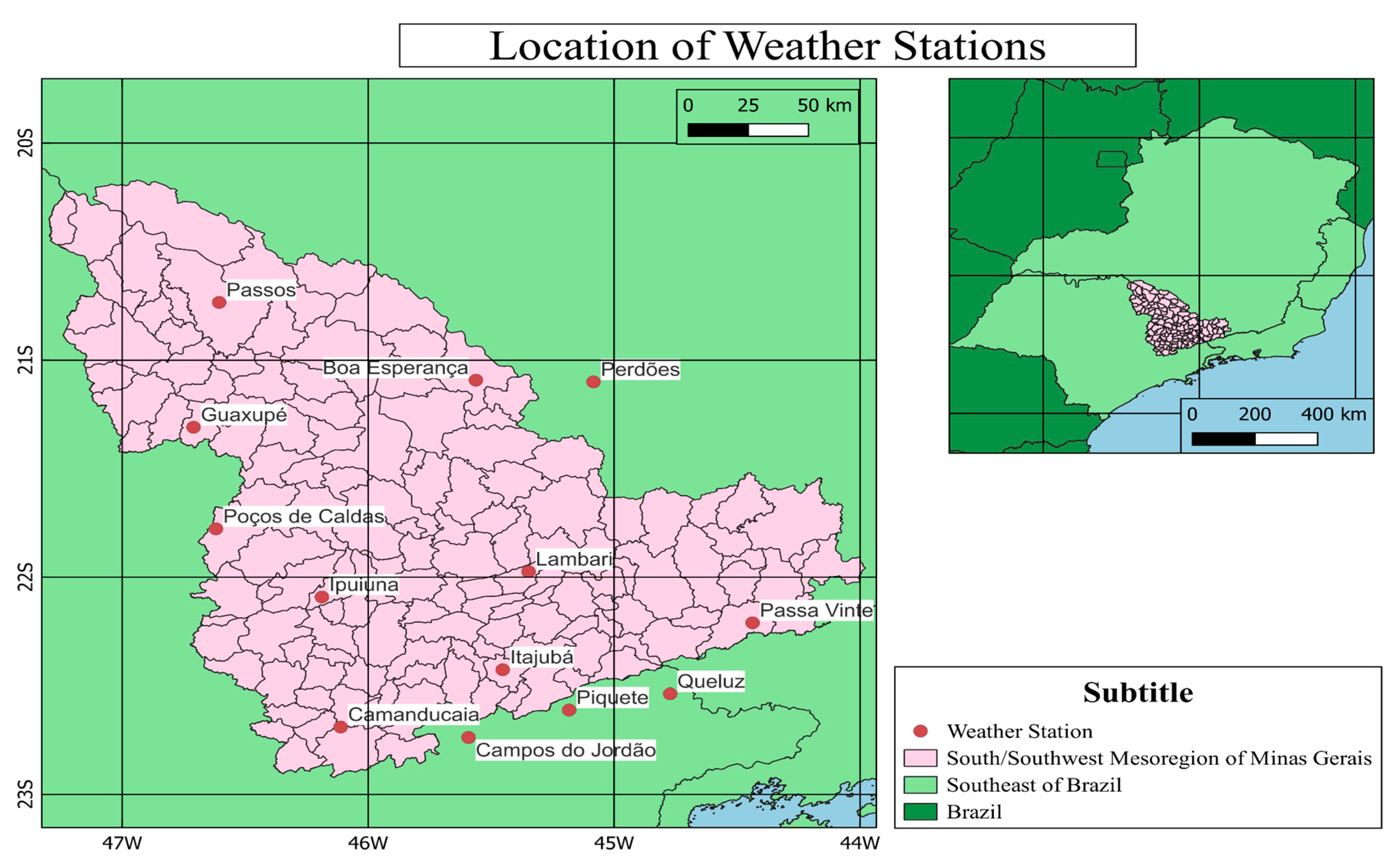
To validate the results obtained with WRF, in addition to the MERGE dataset, precipitation data measured in situ at thirteen weather stations of the National Center for Monitoring and Natural Disaster Alerts (CEMADEN, https://www.gov.br/cemaden/pt-br, (accessed on 13 December 2022)) were used; the precipitation data of these stations were accumulated daily. The zonal and meridional wind components at 850 hPa from ERA5 reanalysis [28] were used as well. The study area and the location of the weather stations considered are shown in Figure 1.
2.2. Numerical Experiments Design
WRF model version 4.4 (WRF4.4), released on August 2022 (https://www2.mmm.ucar.edu/wrf/users/physics/phys_references.html#CU, (accessed on 26 November 2022)), was used to study the impact of different CC parameterizations in simulating rainfall rates during an extreme event in the SMG. The simulations considered two nested grids with horizontal spatial resolutions of 12 km (D-01) and 3 km (D-02), respectively (Figure 2). The shared model configuration considered in all simulations was the same as the one used in the operational forecast system at CEPreMG (Table 2), and the model was driven by GFS forecasts. The simulations were integrated from 0000 Z on 30 December 2021 to 0000 Z on 03 January 2022. The first 12 h of the simulations were discarded to allow the model to spin up. In CEPreMG, the current operational version of WRF considers GF as the cumulus convection parameterization option [29,30].
The simulations differed from each other in their CC parameterization schemes. Five simulations (Table 3) were carried out using the schemes with better performance worldwide described in the literature, as previously shown in Table 1. By assuming that the 3 km grid explicitly allows for solving clouds, the CC parameterizations for this grid were disabled in all simulations [37]. For clarity, the simulations refer to the name of the CC parameterization used, as our goal is to evaluate the impact of the CC parametrization at the coarse domain (D-01) within the high-resolution domain (D-02).
2.3. Performance Analysis
Analysis of the synoptic environment associated with the extreme precipitation event was performed in order to understand the underlying phenomena and atmospheric patterns associated with this event. The spatial distribution of the rainfall was plotted through the MERGE dataset, along with the daily precipitation rates measured by weather stations in the area, and used to characterize the event.
To validate the WRF results, the spatial variability of the rainfall simulated by the different numerical experiments for the D-01 grid was compared to the MERGE dataset. Hence, in order to allow the comparison with the MERGE dataset, the rainfall rates simulated by the WRF model were accumulated from 1200 UTC to 1200 UTC. The similarity of the spatial pattern of the experiments in the D-01 grid and MERGE dataset was measured through spatial correlation and bias. Spatial correlation was computed using the Pearson correlation index (R), which indicates how closely two data series are related to each other. Correlation values vary from −1 to 1, where positive values close to 1 indicate stronger positive correlations and negative values closer to -1 indicate stronger negative correlations [45]. The bias, which represents the difference between simulation and observation (), was applied to compare the daily spatial distribution of precipitation. Thus, a spatial average of the daily accumulated precipitation was performed among all grid points for both MERGE and simulations in the sequence, and the difference model minus MERGE was obtained. The bias indicates the underestimation or overestimation of the model when compared to MERGE data [46]. The vertically integrated moisture flux between 1000 and 100 hPa for the D-01 grid was calculated to allow for analysis of its impact on the formation of the weather event.
For a local analysis, the precipitation simulated through the D-02 grid was compared with in situ measured data. For this comparison, the average of the area around the grid point closest to the weather station was calculated to define the precipitation rate for comparison with the observations. An area of 6 km radius from the grid point was used to calculate this average. To better evaluate the performance of the high-resolution simulations, class intervals for the accumulated daily rainfall rates for the SMG were defined as follows: 0–10 mm—light rain, 11–30 mm—moderate rain, 31–50 mm—heavy rain, and above 50 mm—very heavy rain. The daily accumulated values of the in situ measurements and the WRF results were then associated with the rain categories defined through the thresholds for comparison.
3. Results
3.1. Rainy Period Overview
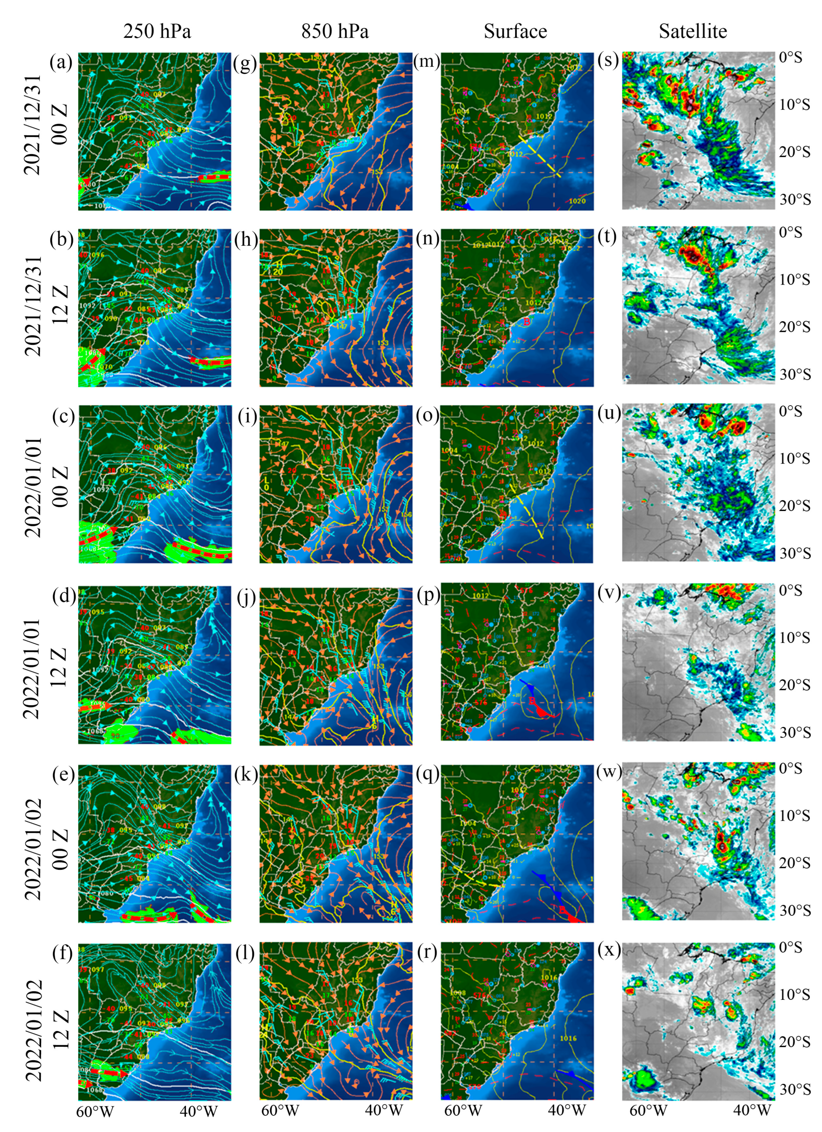
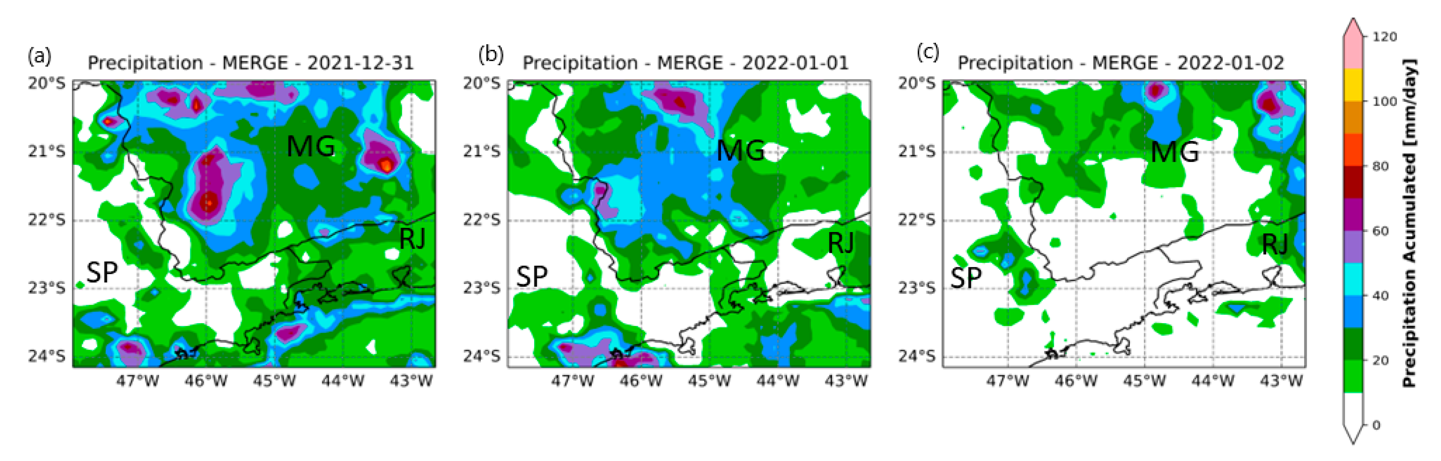
Between December 31 of 2021 and January 2 of 2022, a low-pressure system moved through the coast of SEB (Figure 3m–r). At 250 hPa (Figure 3a–f), with a trough located over the Midwest Brazil and SEB supporting the surface low pressure system. The 850 hPa chart (Figure 3g–l) shows the convergence of winds over the SMG; the branch that reaches the SMG is from Amazonia, while the other is from the Atlantic Ocean. Thus, the transport of moist and warm air to the SMG contributes to atmospheric instability and subsequent cloud formation and precipitation (Figure 3s–x). From December 31st and January 1st, the low surface pressure intensifies (Figure 3p). During these days, the satellite images show an extensive band of cloudiness located between the center of Brazil and the Atlantic Ocean (Figure 3s,t); daily precipitation totals of approximately 60 mm were recorded in the Mantiqueira mountain region (Figure 4). According to [47], values of 60 mm are considered extreme events in Minas Gerais state during the rainy period. Therefore, we can consider the studied period as one of extreme daily precipitation that is dangerous for vulnerable communities leaving near the slope of the mountains.
The spatial distribution of the daily accumulated precipitation obtained from the MERGE dataset between December 31 of 2021 and January 2 of 2022 is shown in Figure 4. The highest precipitation volumes, reaching about 70 mm, were concentrated in the north of the study region. Considering the Mantiqueira mountain range (on the borders between the states of SP, MG, and RJ with southern MG state), the daily precipitation totals showed a variation of 20 to 60 mm between December 31 of 2021 and January 01 of 2022.
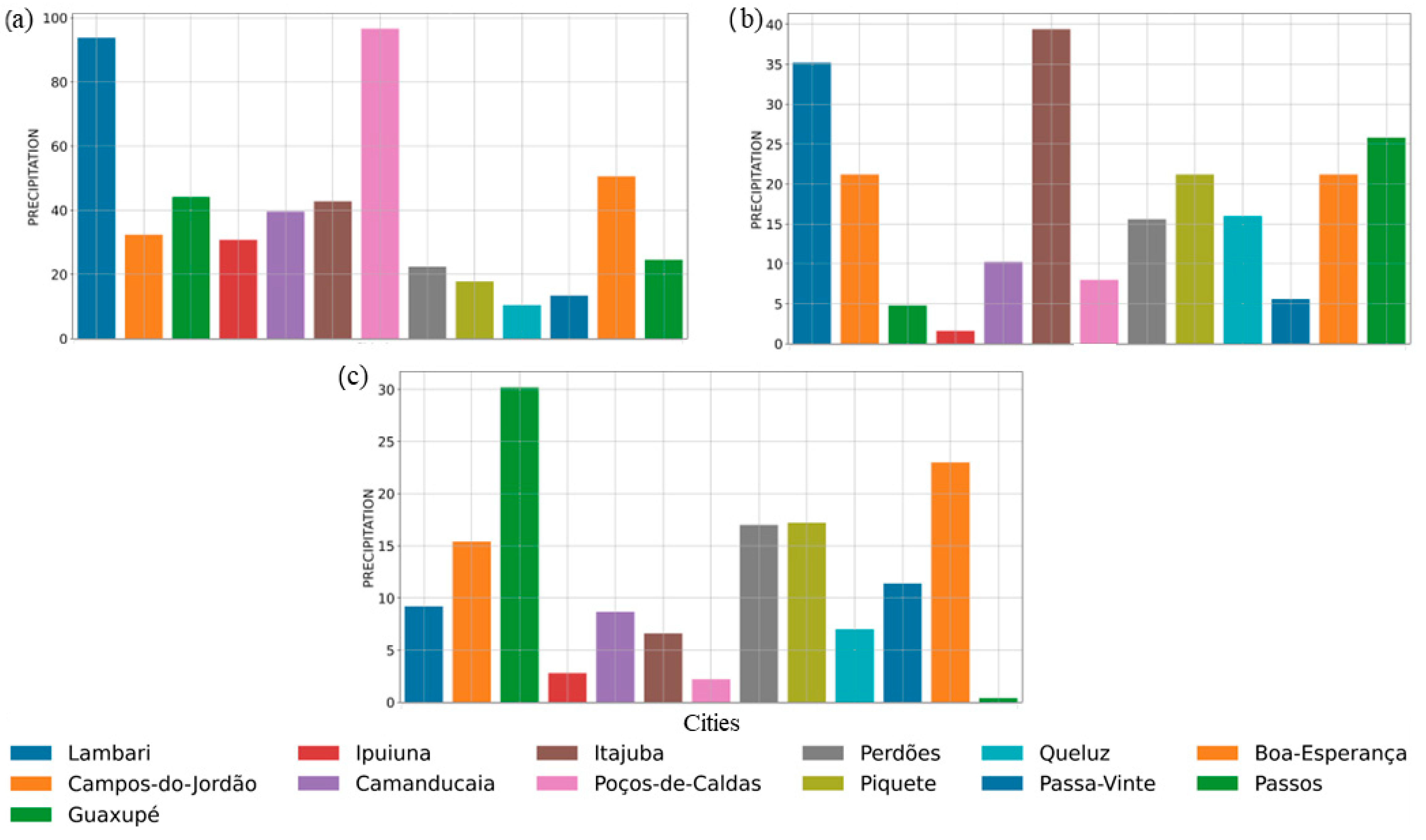
Regions with high volumes of precipitation over the SMG as indicated by the MERGE dataset correspond to the places with the highest volumes recorded through the in situ observations, as shown in Figure 5. As an example, values of 54.6 and 36.2 from the MERGE dataset and 93.8 and 96.6 from in situ observations are respectively revealed for the sites of Lambari and Poços de Caldas on December 31 of 2022. These two locations are far apart within the study region (127 km distant from each other), indicating that the MERGE dataset represents the spatial distribution of the precipitation but underestimates it. Studies such as [48,49,50,51] have shown suitable results when validating the use of MERGE dataset to represent the precipitation spatial patterns associated with specific events in Brazil. However, [50,52] highlighted that the MERGE data underestimate intense precipitation values.
3.2. WRF Evaluation
3.2.1. Domain D-01
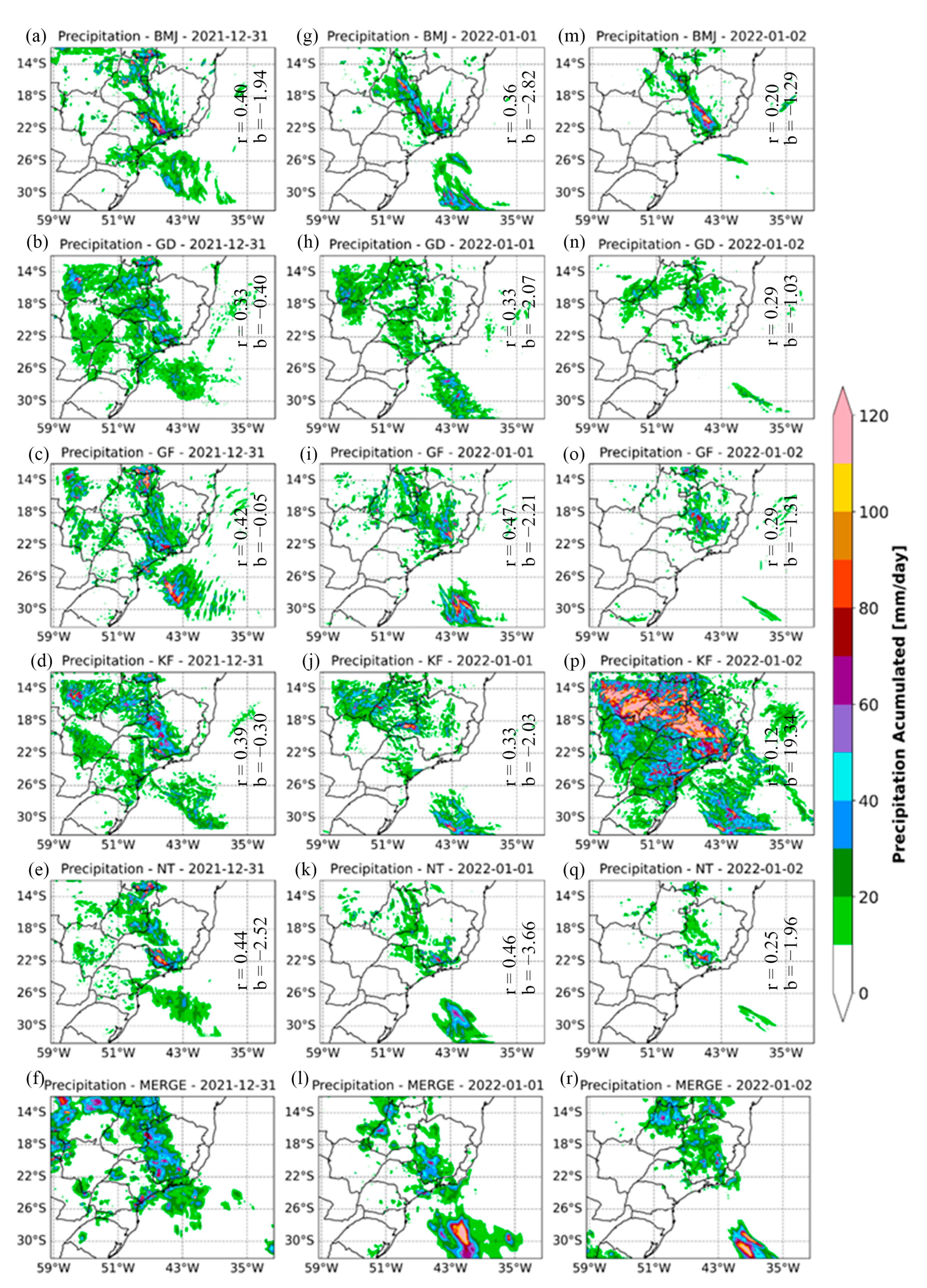
Figure 6 shows the spatial distribution of the total daily precipitation obtained from the different numerical experiments. Several simulations overestimated the precipitation over the South Atlantic Ocean on December 31, while, on this same day there were underestimates near the coast. In general, KF is the CC scheme with the higher overestimates (Figure 6d–p) and NT the one with the higher underestimates (Figure 6e–q). For example, on 02 January 2022 the intensity of the precipitation values was largely overestimated by KF. In the GD simulation (Figure 6n), the precipitation is more spread over the continent compared to the MERGE dataset. BMJ (Figure 6m) and GF (Figure 6o) show more similarities with the MERGE dataset in terms of volumes and spatial distributions.
Although in other regions of the world KF has shown good performance (such as in [53], which mentions that KF may be more accurate in convective precipitation events due to mass conservation, and [21], which reported lower errors and a high probability of detection (POD) when simulating events with extreme precipitation with the KF parameterization option), for our study region KF had lower performance. Moreover, [17] showed underestimation by an average of 12 mm/day of precipitation rates in WRF simulations using GF and KF as CC for Paraiba do Sul River Basin, Brazil.
To quantify the similarity between each experiment and the MERGE dataset, the daily spatial correlation (r) and bias were computed. During the three days, better spatial correlation is obtained with GF CC, which for 1 January 2022 has r = 0.47 (Figure 6c–o). The visual analysis shows that GF is able to represent spatial variability patterns closer to those from the MERGE dataset (Figure 6 f–r). The smallest difference between the model results and MERGE data (bias) was obtained for 31 December 2021, again when GF was used (bias = −0.05). However, as MERGE has a tendency towards underestimation compared to station data, the low bias obtained with GF could indicate that this simulation similarly underestimates the rainfall daily rates. This pattern was evaluated for the high-resolution grid (D-02) through comparison of the model results with local precipitation data.
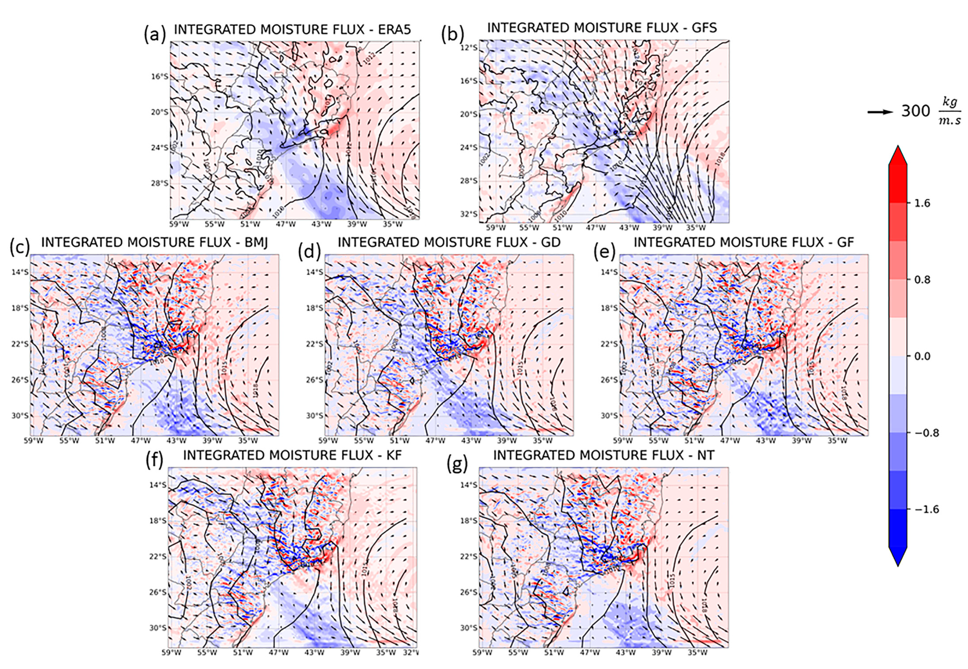
In order to provide a physical explanation of the differences in performance between rainfall simulations in the numerical experiments, Figure 7 presents the average vertically integrated moisture flux divergence and the flux vectors and mean sea level pressure from 31 December to 2 January. The same vertical levels as in the reference datasets and simulations were used in order to facilitate comparison. The vertically integrated moisture flux indicates convergence (negative values) and divergence (positive values) of the flow during the event. For this analysis, the outputs of the WRF model with different CC parameterization options were compared with data from ERA5 reanalysis. The GFS data are shown as well, because they were used as WRF input data to generate initial and boundary conditions required for the simulations. Therefore, a possible bad representation of the moisture flux by GFS could impact its representation in WRF. Due to the higher resolution of the WRF model, its results present further details which cannot be seen in Figure 7a, b, which was plotted using ERA5 and GFS data, respectively. The ERA5 and GFS data (Figure 7a, b) show a strong convergence of moisture between the SMG and São Paulo state. Moisture divergence dominates over the Atlantic Ocean, associated with the winds of the west side of the South Atlantic Subtropical Anticyclone (SASA). Most of the flow starts from the Amazon region, acquires a curvature over Midwest Brazil, and then reaches the SMG. This flow is in part a response to the horizontal pressure gradient between the Amazon Forest and the anomalous low pressure near the Brazilian coast [54,55]. The low-pressure area (1010 hPa) acts as an attractor of the South American Low-level Jet (SALLJ). Compared to ERA5, the GFS forecasts show the same spatial pattern of areas with divergence, and convergence, and flow direction, but presents differences in the isobars near the coast, more intense winds than ERA5 in the SALLJ path, and weaker winds over Paraguay and part of midwestern and southern Brazil. In general, an overestimation of the wind speed produced by GFS data was found by [56] in a comparison with station data for Minas Gerais State, Brazil.
Although WRF was driven by the GFS forecasts, the spatial pattern of the isobars in the experiments were closer to ERA5 (Figure 7c–g). The experiments represented the mean sea level pressure over the ocean associated with the SASA and the low area near the southeastern coast of Brazil well. On the other hand, the experiments showed differences in the divergence of the vertically integrated moisture flow and in the intensity and direction of the flow vectors when compared with ERA5 and GFS. The integrated moisture flux vectors in the path of the SALLJ have a slightly different route, and are weaker than ERA5 and GFS. This may be associated with the dynamics and physics of WRF.
The integrated moisture flux path simulated by GF is more similar to ERA5, as the other simulations show a more meridional orientation in the flux vectors. However, from Figure 7 the reason for this path and consequent better model performance is not clear. We emphasize that the comparison of the experiments with ERA5 indicates that GF represented the moisture flow in the atmosphere better, which resulted in a good precipitation forecast for the SEB in D-01 grid as compared with the MERGE dataset. Previous studies for the same region, such as [17], have indicated that WRF represents the main patterns of ERA5 well, especially the mean sea level pressure and wind intensity at 850 hPa.
3.2.2. Domain D-02
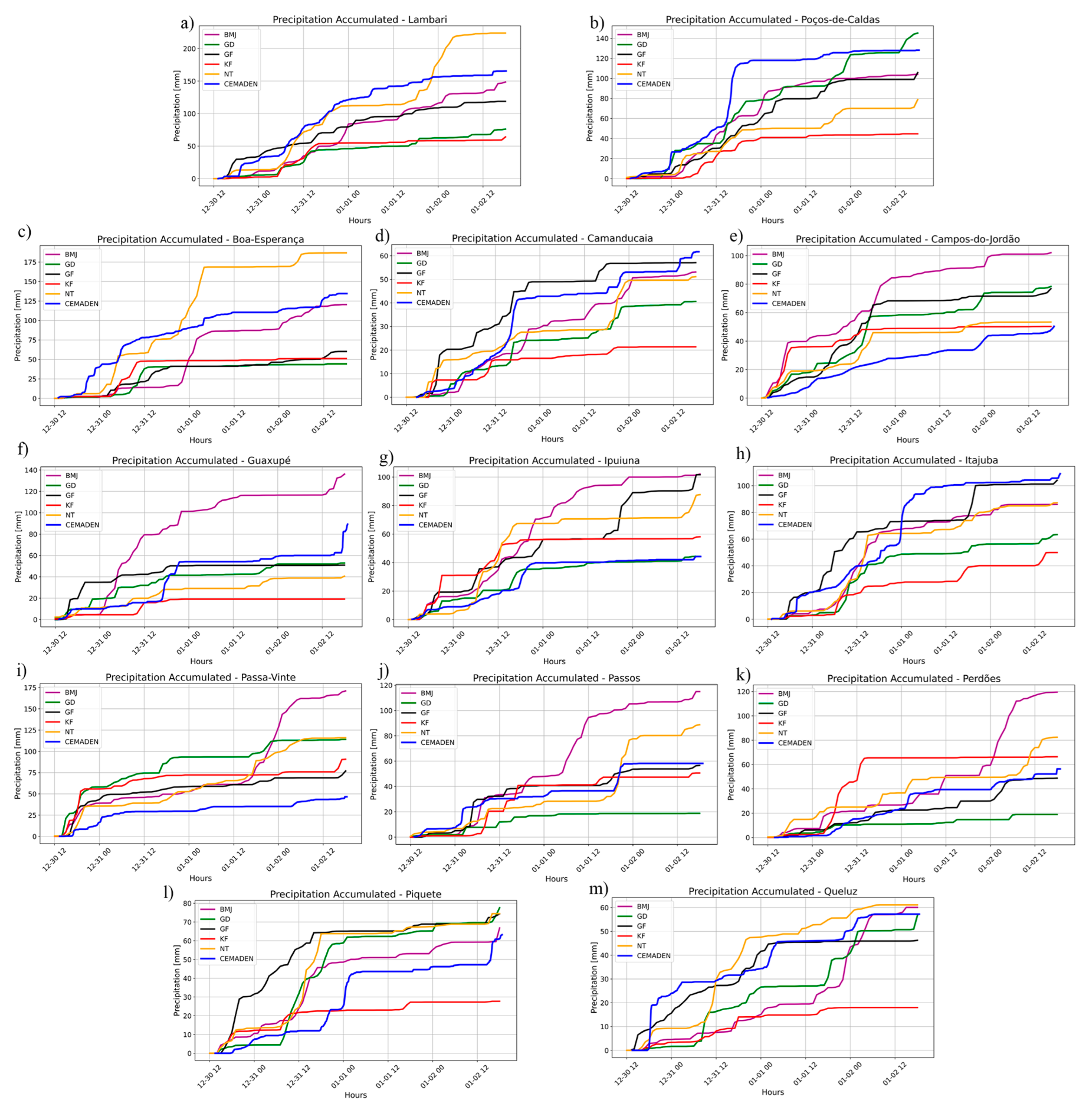
Figure 8 shows the comparison between the hourly precipitation registered in situ at each station and the WRF results extracted from the D-02 grid considering an average of the grid points around the station location. It is important to highlight that the SMG is located in complex mountainous terrain, which increases the difficulties when simulating precipitation with NWP models [57,58,59,60,61].
For brevity, we selected only two stations from Figure 8 to describe the results in more detail, namely, Lambari and Poços de Caldas. The data recorded in Lambari (the blue line in Figure 8a) reveal that there was a precipitation peak during the first 12 h. The NT simulation results, shown by the orange line, obtained better performance when predicting this peak around 0600 Z, while the other CC parameterization simulations results did not show accentuated precipitation peaks. Over the hours, NT overestimated precipitation values at the end of January 2 of 2022. In general, NT satisfactorily represented the hourly and daily accumulated precipitation values for the three days of the event. BMJ (the purple line) presented greater stability of the simulated precipitation compared to NT, as large peaks of precipitation were not simulated in a short time interval. Hence, it provides a good representation of the in situ observations despite the underestimation of the peak values, as verified by [62], where the BMJ parameterization presented better results for different microphysics parameterization options, including for WSM5, currently used in the operation in CEPreMG [26]. GF had better performance in the first three days compared to BMJ, and although GF underestimated the precipitation, it is able to simulate the temporal variability.
In Poços de Caldas, the weather station (the blue line in Figure 8b) recorded an accumulated precipitation rate for the three days that was above 120 mm. Unlike Lambari, NT (the yellow line) underestimated the rainfall values. The precipitation peak in Poços de Caldas was recorded shortly after 1200 Z on December 31 of 2021. The CC parameterization that best represented the accumulated precipitation was BMJ, with values higher than 90 mm for the accumulated precipitation during the entire event even without simulating the precipitation peak, followed by GF. In general, the WRF simulations underestimated the accumulated precipitation, corroborating results found in other studies for mountain regions [63,64,65,66,67,68]. In [63], the authors paid attention to the fact that each extreme event has different characteristics from the others. In this way, there is no combination of parameterization schemes that can be called the best for all simulated events.
From Figure 8, it is clear that there is no one better or worse CC parameterization scheme. Focusing on GF, however, it has reasonable performance (not necessarily better performance, but consistent at almost all stations) compared to the other CC schemes. Only for Boa Esperança, Campos de Jordão, Ipuiuna, and Piquete GF does it show lower ability (Figure 8c, e, g, l). The complex terrain and land use characteristics at these sites could explain these results. Boa Esperança is located close to large water reservoir (Furnas), Piquete is located in the base of Serra da Mantiqueira, and Campos do Jordão and Ipuiuna are located at higher altitudes (higher than 1600 and 1200 m, respectively). The influence of the terrain on the precipitation rates simulated by WRF was previously pointed out by [17,69].
For a more precise validation of the experiments, daily rainfall was separated into classes, as shown in Table 4 and Table 5 for Lambari and Poços de Caldas, respectively (the results for the other sites are presented in the Supplementary Materials). For Lambari, the comparison between the model results and the rainfall classes highlights the general underestimation of the recorded precipitation values by the model. Similar results were obtained by other studies in the same region, such as [17,65]. It is possible to verify that no parameterization stands out as the most appropriate when carrying out this comparison. It appears that for 2 January 2022 the model had difficulty representing the de-intensification of the system and resulting decrease in precipitation rates. Similar results were found for all sites, as can be seen in the tables available as Supplementary Material. These results corroborate the difficulties associated with rain forecasting for specific locations.
4. Conclusions
In the South of Minas Gerais state (SMG), located in the southeastern region of Brazil, the Center for Weather and Climate Prediction of Minas Gerais (CEPreMG) has run a daily the WRF model since 2017 to enhance weather forecasting for the region. However, following its implementation only a few studies have been carried out to evaluate which are the best physical parameterization schemes that should be used to better simulate the rainfall patterns and rates in the region, which has some of the most complex terrain in the country and has reported severe extreme precipitation events with significant social economic impacts throughout recent decades. Thus, this study aimed to use the same settings as the WRF model that is in operational mode, with the exception of cumulus convection, in order to evaluate which is the best cumulus convection scheme that represents extreme precipitation episodes in the SMG. For this purpose, the extreme precipitation event registered between 31 December 2021 and 2 January 2022 was chosen.
For the grid with coarse resolution (D–01), the results showed that the precipitation simulated by the GF was more similar in spatial distribution and intensity to the MERGE reference dataset. However, this dataset is known to underestimate rainfall rates when compared to in situ measurements. Hence, the representation of the average vertically integrated moisture flux divergence and the flux vectors and mean sea level pressure by WRF was compared with ERA5 reanalysis and GFS data, which were used as inputs to the WRF model. The GFS forecasting results showed the same spatial pattern as ERA5 in terms of areas with divergence, convergence, and flow direction, but presented differences in the isobars near the coast, more intense winds in the SALLJ path, and weaker winds over Paraguay and part of midwestern and southern Brazil. Therefore, this could be a source of error for WRF simulations and should be explored in future numerical experiments. When the analysis was performed for the D-02 domain, GF was the scheme that presented more coherent results representing the accumulated rainfall rates in comparison with observations. These results indicate that the GF CC scheme currently in use with the WRF at CEPreMG is the most adequate for precipitation forecasting in the region.
Supplementary Materials
The following supporting information can be downloaded at: https://www.mdpi.com/article/10.3390/atmos14081276/s1, Table S1: Classification of intensity rain to Boa Esperança city to period study of 31 December 2021 to 2 January 2022; Table S2: Classification of intensity rain to Camanducaia city to period study of 31 December 2021 to 2 January 2022; Table S3: Classification of intensity rain to Campos do Jordão city to period study of 31 December 2021 to 2 January 2022; Table S4: Classification of intensity rain to Guaxupé city to period study of 31 December 2021 to 2 January 2022; Table S5: Classification of intensity rain to Ipuiuna city to period study of 31 December 2021 to 2 January 2022; Table S6: Classification of intensity rain to Itajubá city to period study of 31 December 2021 to 2 January 2022; Table S7: Classification of intensity rain to Passa Vinte city to period study of 31 December 2021 to 2 January 2022; Table S8: Classification of intensity rain to Passos city to period study of 31 December 2021 to 2 January 2022; Table S9: Classification of intensity rain to Perdões city to period study of 31 December 2021 to 2 January 2022; Table S10: Classification of intensity rain to Piquete city to period study of 31 December 2021 to 2 January 2022; Table S11: Classification of intensity rain to Queluz city to period study of 31 December 2021 to 2 January 2022.
Author Contributions
Methodology, D.W.G., M.S.R., and V.S.B.C.; Software, D.W.G.; Formal analysis, D.W.G.; Writing—original draft, D.W.G.; Writing—review and editing, M.S.R. and V.S.B.C.; Visualization, D.W.G.; Project administration, M.S.R. All authors have read and agreed to the published version of the manuscript.
Funding
This work was financially supported by the Minas Gerais State Research Support (FAPEMIG, No: APQ-00134-17).
Data Availability Statement
Not applicable.
Acknowledgments
This work was supported by the Coordenação de Aperfeiçoamento de Pessoal de Nível Superior (CAPES, Coordination for the Improvement of Higher Education Personnel), by the Fundação de Amparo à Pesquisa do Estado de Minas Gerais (FAPEMIG, Minas Gerais State Research Support Foundation) and Conselho Nacional de Desenvolvimento Científico e Tecnológico (CNPq).
Conflicts of Interest
The authors declare no conflict of interest.
References
- Alcântara, E.; Marengo, J.A.; Mantovani, J.; Londe, L.; San, R.L.Y.; Park, E.; Lin, Y.N.; Mendes, T.; Cunha, A.P.; Pampuch, L.; et al. Deadly disasters in Southeastern South America: Flash floods and landslides of February 2022 in Petrópolis, Rio de Janeiro. Nat. Hazards Earth Syst. Sci. 2022, 23, 1157–1175. [Google Scholar] [CrossRef]
- Haddad, E.A.; Teixeira, E. Economic impacts of natural disasters in megacities: The case of floods in São Paulo, Brazil. Habitat Intern. 2015, 45, 106–113. [Google Scholar] [CrossRef] [Green Version]
- Oliveira, P.D.; Santos e Silva, C.M.; Lima, K.C. Climatology and trend analysis of extreme precipitation in subregions of Northeast Brazil. Theor. Appl. Clim. 2017, 130, 77–90. [Google Scholar] [CrossRef]
- Lima, S.S.; Armond, N.B. Rainfall in Metropolitan Region of Rio de Janeiro: Characterization, extreme events and trends. Soc. Nat. 2022, 34, 1–19. [Google Scholar] [CrossRef]
- Marengo, J.A.; Seluchi, M.E.; Cunha, A.P.; Cuartas, L.A.; Goncalves, D.; Sperling, V.B.; Ramos, A.M.; Dolif, G.; Saito, S.; Bender, F.; et al. Heavy rainfall associated with floods in southeastern Brazil in November–December 2021. Nat. Haz. 2023, 116, 3617–3644. [Google Scholar] [CrossRef]
- Avila-Diaz, A.; Benezoli, V.; Justino, F.; Torres, R.; Wilson, A. Assessing current and future trends of climate extremes across Brazil based on reanalyzes and earth system model projections. Clim. Dyn. 2020, 55, 1403–1426. [Google Scholar] [CrossRef]
- Gu, G.; Adler, R.F. Observed variability and trends in global precipitation during 1979–2020. Clim. Dyn. 2022, 61, 131–150. [Google Scholar] [CrossRef]
- Reboita, M.S.; da Rocha, R.P.; Souza, C.A.D.; Baldoni, T.C.; Silva, P.L.L.D.S.; Ferreira, G.W.S. Future projections of extreme precipitation climate indices over South America based on CORDEX-CORE multimodel ensemble. Atmos 2022, 13, 1463. [Google Scholar] [CrossRef]
- Zilli, M.T.; Carvalho, L.M.; Liebmann, B.; Silva Dias, M.A. A comprehensive analysis of trends in extreme precipitation over southeastern coast of Brazil. Int. J. Clim. 2017, 37, 2269–2279. [Google Scholar] [CrossRef]
- Silva, P.L.L.; Baldoni, T.C.; Ribeiro, G.T.S.; Reboita, M.S. Ambiente em escala sinótica associado ao extremo de chuva no litoral de São Paulo nos dias 18 e 19 de fevereiro de 2023. In Proceedings of the IX Seminário de Recursos Naturais, Itajubá, Brazil, 5–7 June 2023. [Google Scholar]
- Instituto Brasileiro de Geografia e Estatística—IBGE. Censo Demográfico 2022. 2023. Available online: https://www.ibge.gov.br/estatisticas/sociais/populacao/22827-censo-demografico-2022.html?=&t=resultados (accessed on 15 February 2023).
- Bartolomei, F.R.; Ribeiro, J.G.M.; Reboita, M.S. Eventos Extremos de Precipitação no Sudeste do Brasil: Verão 2021/2022. Rev. Bras. Geogr. Fis. 2023. (accepted). [Google Scholar]
- Silveira, G.L.; Xavier, R.G.; Reboita, M.S.; Reis, A.L. Análise do Evento Extremo de Precipitação ocorrido em Petrópolis-RJ no dia 15 de fevereiro de 2022. In Proceedings of the IX Seminário de Recursos Naturais 2023, Itajubá, Brazil, 5–7 June 2023. [Google Scholar]
- Instituto Nacional de Meteorologia—INMET. Normais Climátológicas—Gráficos Climatológicos. 2023. Available online: https://clima.inmet.gov.br/GraficosClimatologicos/DF/83377 (accessed on 15 February 2023).
- Teodoro, T.A.; Reboita, M.S.; Llopart, M.; Da Rocha, R.P.; Ashfaq, M. Climate change impacts on the South American monsoon system and its surface–atmosphere 564 processes through RegCM4 CORDEX-CORE projections. Earth Syst. Env. 2021, 5, 825–847. [Google Scholar] [CrossRef]
- Almeida Dantas, V.; Silva Filho, V.P.; Santos, E.B.; Gandu, A.W. Testando diferentes esquemas da Parametrização Cumulus do modelo WRF; para a região norte Nordeste do Brasileiro (Testing different WRF Cumulus parameterization schemes for the north-eastern region of Brazil). Rev. Bras. Geogr. Fis. 2019, 12, 754–767. [Google Scholar] [CrossRef]
- Campos, B. Sensibilidade de Parametrizações de Convecção Cumulus e Microfísica de Nuvens em Eventos Extremos de Precipitação na Bacia do Rio Paraíba do Sul. Master’s Thesis, (Mestrado em Meio Ambiente e Recursos Hídricos), Universidade Federal de Itajubá, Itajubá, Brazil, 2023. [Google Scholar]
- Jeworrek, J.; West, G.; Stull, R. Evaluation of cumulus and microphysics parameterizations in WRF across the convective gray zone. Weather. Forecast. 2019, 34, 1097–1115. [Google Scholar] [CrossRef]
- Prein, A.F.; Langhans, W.; Fosser, G.; Ferrone, A.; Ban, N.; Goergen, K.; Keller, M.; Tölle, M.; Gutjahr, O.; Feser, F.; et al. A review on regional convection-permitting climate modeling: Demonstrations, prospects, and challenges. Rev. Geophys. 2015, 53, 323–361. [Google Scholar] [CrossRef] [PubMed] [Green Version]
- Gilliland, E.K.; Rowe, C.M. A comparison of cumulus parameterization schemes in the WRF model. In Proceedings of the 87th AMS Annual Meeting & 21th Conference on Hydrology, San Antonio, TX, USA, 13–18 January 2007; Volume 2. [Google Scholar]
- Pennelly, C.; Reuter, G.; Flesch, T. Verification of the WRF model for simulating heavy precipitation in Alberta. Atmos. Res. 2014, 135, 172–192. [Google Scholar] [CrossRef]
- Stergiou, I.; Tagaris, E.; Sotiropoulou, R.-E.P. Sensitivity Assessment of WRF Parameterizations over Europe. Proceedings 2017, 1, 119. [Google Scholar]
- Hasan, M.A.; Islam, A.S. Evaluation of microphysics and cumulus schemes of WRF for forecasting of heavy monsoon rainfall over the southeastern hilly region of Bangladesh. Pure Appl. Geophys. 2018, 175, 4537–4566. [Google Scholar] [CrossRef]
- Otieno, G.; Mutemi, J.N.; Opijah, F.J.; Ogallo, L.A.; Omondi, M.H. The sensitivity of rainfall characteristics to cumulus parameterization schemes from a WRF model. Part I: A case study over East Africa during wet years. Pure Appl. Geophys. 2020, 177, 1095–1110. [Google Scholar] [CrossRef]
- Nasrollahi, N.; AghaKouchak, A.; Li, J.; Gao, X.; Hsu, K.; Sorooshian, S. Assessing the impacts of different WRF precipitation physics in hurricane simulations. Weather. Forecast. 2012, 27, 1003–1016. [Google Scholar] [CrossRef] [Green Version]
- Rozante, J.R.; Moreira, D.S.; de Goncalves, L.G.G.; Vila, D.A. Combining TRMM and surface observations of precipitation: Technique and validation over South America. Weather. Forecast. 2010, 25, 885–894. [Google Scholar] [CrossRef] [Green Version]
- Skamarock, C.; Klemp, J.B.; Dudhia, J.; Gill, D.O.; Liu, Z.; Berner, J.; Wang, W.; Powers, J.G.; Duda, M.G.; Barker, D.M.; et al. A Description of the Advanced Research WRF Model Version 4. NCAR Tech Note. NCAR/TN–556+ STR; National Center for Atmospheric Research: Boulder, Colorado, USA, 2021. [Google Scholar]
- Hersbach, H.; Bell, B.; Berrisford, P.; Hirahara, S.; Horányi, A.; Muñoz-Sabater, J.; Nicolas, J.; Peubey, C.; Radu, R.; Schepers, D.; et al. The ERA5 global reanalysis. Q. J. R. Meteorol. Soc. 2020, 146, 1999–2049. [Google Scholar] [CrossRef]
- Araújo, A.A.; Garcia, D.W.; Monteiro, J.R.; Miguel, T.V.; Campos, B.; Carvalho, V.S.B.; Reboita, M.S. Avaliação do modelo Weather Research and Forecasting (WRF) na simulação operacional de um evento de frente fria no sudeste do Brasil. Rev. Bras. Geogr. Fis. 2023, 16, 805–817. [Google Scholar] [CrossRef]
- Campos, B.; Carvalho, V.S.B.; Reboita, M.S. The numeric-operational weather forecast system for the southern region of the Minas Gerais state: Comparisons with observed data. Rev. Bras. Geogr. Fis. 2016, 9, 1017–1029. [Google Scholar] [CrossRef] [Green Version]
- Hong, S.; Dudhia, J.; Chen, S. A revised approach to ice microphysical processes for the bulk parameterization of clouds and precipitation. Mon. Weather. Rev. 2004, 132, 103–120. [Google Scholar] [CrossRef]
- Hong, S.; Dudhia, J. A new vertical diffusion package with an explicit treatment of entrainment processes. Mon. Weather. Rev. 2006, 134, 2318–2341. [Google Scholar] [CrossRef] [Green Version]
- Jiménez, P.A.; Dudhia, J.; González-Rouco, J.F.; Navarro, J.; Montávez, J.P.; García-Bustamante, E. A Revised Scheme for the WRF Surface Layer Formulation. Mon. Weather. Rev. 2012, 140, 898–918. [Google Scholar] [CrossRef] [Green Version]
- Mukul Tewari, N.C.A.R.; Tewari, M.; Chen, F.; Wang, W.; Dudhia, J.; LeMone, M.A.; Mitchell, K.; Ek, M.; Gayno, G.; Wegiel, J.; et al. Implementation and verification of the unified NOAH land surface model in the WRF model. In Proceedings of the 20th conference on weather analysis and forecasting/16th conference on numerical weather prediction, Seattle, WA, USA, 10–15 January 2004; pp. 11–15. [Google Scholar]
- Dudhia, J. Numerical Study of Convection Observed during the Winter Monsoon Experiment Using a Mesoscale Two-Dimensional Model. J. Atmos. Sci. 1989, 46, 3077–3107. [Google Scholar] [CrossRef]
- Mlawer, J.E.; Taubman, S.J.; Brown, P.D.; Iacono, M.J.; Clough, S.A. Radiative transfer for inhomogeneous atmospheres: RRTM, a validated correlated-k model for the longwave. J. Geophys. Res. Atmos. 1997, 102, 16663–16682. [Google Scholar] [CrossRef] [Green Version]
- Weisman, M.L.; Skamarock, W.C.; Klemp, J.B. The resolution dependence of explicitly modeled convective systems. Mon. Weather. Rev. 1997, 125, 527–548. [Google Scholar] [CrossRef]
- Kain, J. The Kain–Fritsch convective parameterization: An update. J. Appl. Meteor. 2004, 43, 170–181. [Google Scholar] [CrossRef]
- Kain, J.; Fritsch, J. A one-dimensional entraining/detraining plume model and its application in convective parameterization. J. Atmos. Sci. 1990, 47, 2784–2802. [Google Scholar] [CrossRef]
- Kain, J.; Fritsch, J. Convective parameterization for mesoscale models: The Kain–Fritsch scheme. In The Representation of Cumulus Convection in Numerical Models; American Meteorological Society: Boston, MA, USA, 1993; pp. 165–170. [Google Scholar]
- Janjic, Z.I. The Step–Mountain Eta Coordinate Model: Further developments of the convection, viscous sublayer, and turbulence closure schemes. Mon. Weather. Rev. 1993, 122, 927–945. [Google Scholar] [CrossRef]
- Grell, G.A.; Devenyi, D. A generalized approach to parameterizing convection combining ensemble and data assimilation techniques. Geophys. Res. Lett. 2002, 29, 38-1–38-4. [Google Scholar] [CrossRef] [Green Version]
- Grell, G.A.; Freitas, S.R. A scale and aerosol aware stochastic convective parameterization for weather and air quality modeling. Atmos. Chem. Phys. 2014, 14, 5233–5250. [Google Scholar] [CrossRef] [Green Version]
- Zhang, C.; Wang, Y. Projected Future Changes of Tropical Cyclone Activity over the Western North and South Pacific in a 20-km-Mesh Regional Climate Model. J. Clim. 2017, 30, 5923–5941. [Google Scholar] [CrossRef]
- Wilks, D.S. Statistical Methods in the Atmospheric Sciences; Academic Press: Cambridge, MA, USA, 2011. [Google Scholar]
- Saldanha, C.B.; Radin, B.; Cardoso, M.A.G.; Rippel, M.L.; Fonseca, L.L.D.; Rodriguez, F. Comparação dos dados de precipitação gerados pelo GPCP vs Observados para o estado do Rio Grande do Sul. Rev. Bras. Meteorol. 2015, 30, 415–422. [Google Scholar] [CrossRef]
- dos Reis, A.L.; Silva, M.S.; Regis, M.V.; da Silveira, W.W.; de Souza, A.C.; Reboita, M.S.; Silveira, V. Climatologia e eventos extremos de precipitação no estado de Minas Gerais (Climatology and extreme rainfall events in the state of Minas Gerais). Rev. Bras. Geogr. Fis. 2018, 11, 652–660. [Google Scholar] [CrossRef]
- Munar, A.; Collischonn, W. Simulação Hidrológica na Bacia do rio Piratini, Rio Grande do Sul, a partir de dados de chuva observada e dados de chuva derivados do produto MERGE. 2014. Available online: https://www.researchgate.net/publication/324216200_Simulacao_Hidrologica_na_Bacia_do_rio_Piratini_Rio_Grande_do_Sul_a_partir_de_dados_de_chuva_observada_e_dados_de_chuva_derivados_do_produto_MERGE#fullTextFileContent (accessed on 22 May 2023).
- Torres, F.; Ferreira, G.W.S.; Kuki, C.A.C.; Vasconcellos, B.T.C.; Freitas, A.A.; Silva, P.N.; Souza, C.A.; Reboita, M.S. Validação de diferentes bases de dados de precipitação nas bacias hidrográficas do Sapucaí e São Francisco. Rev. Bras. Clim. 2020, 27, 368–404. [Google Scholar]
- BATISTA, P.D.S. Validação dos dados de precipitação pluvial do produto Merge para a Amazônia Central. Ph.D. Dissertation, Universidade Federal do Oeste do Pará, Santarém, Portugal, 2019. [Google Scholar]
- Salviano, M.F. Comparação entre Estimativas de Precipitação com Satélite e Dados Observados para o Evento de Janeiro de 2020 em Bacias no Sudeste do Brasil. In Proceedings of the II Encontro Nacional de Desastres Hídricos, Online, 15–18 December 2020. [Google Scholar]
- Vila, D.A.; Goncalves, L.G.G.; Toll, D.L.; Rozante, J.R. Statistical evaluation of combined daily gauge observations and rainfall satellite estimates over continental South America. J. Hydrol. 2009, 10, 533–543. [Google Scholar] [CrossRef]
- Gochis, D.J.; Shuttleworth, W.J.; Yang, Z.L. Sensitivity of the modeled North American monsoon regional climate to convective parameterization. Mon. Weather. Rev. 2002, 130, 1282–1298. [Google Scholar] [CrossRef]
- Campetella, C.M.; Possia, N.E. Upper-level cut-off lows in southern South America. Met. Atmos. Phys. 2007, 96, 181–191. [Google Scholar] [CrossRef]
- Reboita, M.S.; Krusche, N.; Ambrizzi, T.; Rocha, R.P. Entendendo o Tempo e o Clima na América do Sul. Available online: https://periodicos.sbu.unicamp.br/ojs/index.php/td/article/view/8637425 (accessed on 9 April 2023). [CrossRef] [Green Version]
- Oliveira Filho, R.A.; Carvalho, V.S.B.; Reboita, M.S. Evaluating the Global Forecast System (GFS) for energy management over Minas Gerais State (Brazil) against in-situ observations. Atmósfera 2022, 35, 357–376. [Google Scholar] [CrossRef]
- Chow, F.K.; Schär, C.; Ban, N.; Lundquist, K.A.; Schlemmer, L.; Shi, X. Crossing multiple gray zones in the transition from mesoscale to microscale simulation over complex terrain. Atmosphere 2019, 10, 274. [Google Scholar] [CrossRef] [Green Version]
- Rauber, R.M.; Geerts, B.; Xue, L.; French, J.; Friedrich, K.; Rasmussen, R.M.; Tessendorf, S.A.; Blestrud, D.R.; Kunkel, M.L.; Parkinson, S. Wintertime orographic cloud seeding—A review. J. Appl. Meteor. 2019, 58, 2117–2140. [Google Scholar] [CrossRef]
- Wiersema, D.J.; Lundquist, K.A.; Chow, F.K. Development of a Multiscale Modeling Framework for Urban Simulations in the Weather Research and Forecasting Model; Lawrence Livermore National Lab. (LLNL): Livermore, CA, USA, 2018. [Google Scholar]
- Wiersema, D.J.; Lundquist, K.A.; Chow, F.K. Mesoscale to microscale simulations over complex terrain with the immersed boundary method in the Weather Research and Forecasting Model. Mon. Weather. Rev. 2020, 148, 577–595. [Google Scholar] [CrossRef]
- Jeworrek, J.; West, G.; Stull, R. WRF precipitation performance and predictability for systematically varied parameterizations over complex terrain. Weather. Forecast. 2021, 36, 893–913. [Google Scholar] [CrossRef]
- Sikder, S.; Hossain, F. Assessment of the weather research and forecasting model generalized parameterization schemes for advancement of precipitation forecasting in monsoon-driven river basins. J. Adv. Model. Earth Syst. 2016, 8, 1210–1228. [Google Scholar] [CrossRef] [Green Version]
- Merino, A.; García-Ortega, E.; Navarro, A.; Sánchez, J.L.; Tapiador, F.J. WRF hourly evaluation for extreme precipitation events. Atmos. Res. 2022, 274, 106215. [Google Scholar] [CrossRef]
- Choubin, B.; Malekian, A.; Golshan, M. Application of several data-driven techniques to predict a standardized precipitation index. Atmósfera 2016, 29, 121–128. [Google Scholar] [CrossRef] [Green Version]
- Calado, R.N.; Dereczynski, C.P.; Chou, S.C.; Suei, G.; Oliveira Moura, J.D.; Silva Santos, V.R. Avaliação do Desempenho das Simulações por Conjunto do Modelo Eta-5km para o Caso de Chuva Intensa na Bacia do Rio Paraíba do Sul em janeiro de 2000. Rev. Bras. Meteor. 2018, 33, 83–96. [Google Scholar] [CrossRef] [Green Version]
- Mu, Z.; Zhou, Y.; Peng, L.; He, Y. Numerical rainfall simulation of different WRF parameterization schemes with different spatiotemporal rainfall evenness levels in the Ili region. Water 2019, 11, 2569. [Google Scholar] [CrossRef] [Green Version]
- Tewari, M.; Chen, F.; Dudhia, J.; Ray, P.; Miao, S.; Nikolopoulos, E.; Treinish, L. Understanding the sensitivity of WRF hindcast of Beijing extreme rainfall of 21 July 2012 to microphysics and model initial time. Atmos. Res. 2022, 271, 106085. [Google Scholar] [CrossRef]
- Glisan, J.M.; Jones, R.; Lennard, C.; Castillo Pérez, N.I.; Lucas-Picher, P.; Rinke, A.; Solman, S.; Gutowski, W.J., Jr. A metrics-based analysis of seasonal daily precipitation and near-surface temperature within seven Coordinated Regional Climate Downscaling Experiment domains. Atmos. Sci. Lett. 2019, 20, e897. [Google Scholar] [CrossRef] [Green Version]
- Jing, X.; Geerts, B.; Wang, Y.; Liu, C. Evaluating seasonal orographic precipitation in the interior western United States using gauge data, gridded precipitation estimates, and a regional climate simulation. J. Hydrometeorol. 2017, 18, 2541–2558. [Google Scholar] [CrossRef]
Figure 1.
Study area showing the SMG (rosa) and location of the weather stations (red dots): Boa Esperança (MG), Camanducaia (MG), Campos do Jordão (SP), Guaxupé (MG), Ipuiúna (MG), Itajubá (MG), Lambari (MG), Passa Vinte (MG), Passos (MG), Perdões (MG), Piquete (SP), Poços de Caldas (MG), and Queluz (SP).

Figure 2.
WRF outer (D-01) and internal (D-02) domains.

Figure 3.
Synoptic charts at: (a–f) 250 hPa, showing the streamlines and wind intensity stronger than 70 knots in green; the upper-level jet is indicated by the red dashed line; (g–l) 850 hPa, showing the streamlines (orange lines), wind barbs (knots), and geopotential height (meters, yellow lines); and (m–r) surface, showing the mean sea level pressure (hPa, yellow lines), low pressure (B), and cold and warm fronts; and (s–x) satellite images channel 13 (°C) (a,g,m,s) for 0000 Z Dezember 31 of 2021, (b,h,n,t) 1200 Z Dezember 31 of 2021, (c,i,o,u) 0000 Z January 01 of 2022, (d,j,p,v), 1200 Z January 01 of 2022, (e,k,q,w) 0000 Z January 02 of 2022, and (f,l,r,x) 1200 Z of January 02 of 2022.

Figure 4.
Total daily precipitation (mm/day) from the MERGE dataset for (a) December 31 of 2021, (b) January 01, and (c) January 02 of 2022.
Figure 4.
Total daily precipitation (mm/day) from the MERGE dataset for (a) December 31 of 2021, (b) January 01, and (c) January 02 of 2022.

Figure 5.
Total daily precipitation (mm/day) registered by weather stations on (a) December 31 of 2021, (b) January 1 of 2022, and (c) January 2 of 2022.
Figure 5.
Total daily precipitation (mm/day) registered by weather stations on (a) December 31 of 2021, (b) January 1 of 2022, and (c) January 2 of 2022.

Figure 6.
Total daily precipitation (mm/day) simulated by (a,g,m) BMJ, (b,h,m) GD, (c,i,o) GF, (d,j,p) KF, (e,k,q) NT, and (f,l,r) MERGE dataset on (a–f) December 31 of 2021, (g–l) January 01 of 2022, and (m–r) January 02 of 2022. At the right side of the figures, the spatial correlation (r) and bias (b) are shown.

Figure 7.
Average between 31 December 2021 and January 2 of 2022 of the vertically integrated moisture flux divergence between 1000 and 100 hPa (kg/m2.s, shaded), showing flux vectors (kg/m.s) and mean sea level pressure (hPa, black lines).
Figure 7.
Average between 31 December 2021 and January 2 of 2022 of the vertically integrated moisture flux divergence between 1000 and 100 hPa (kg/m2.s, shaded), showing flux vectors (kg/m.s) and mean sea level pressure (hPa, black lines).

Figure 8.
Comparison between the hourly precipitation rates (mm/hour) measured in situ (blue line) and simulated with WRF model experiments: BMJ (purple line), GD (green line), GF (black line), KF (red line), and NT (yellow line) for (a) Lambari and (b) Poços de Caldas.
Figure 8.
Comparison between the hourly precipitation rates (mm/hour) measured in situ (blue line) and simulated with WRF model experiments: BMJ (purple line), GD (green line), GF (black line), KF (red line), and NT (yellow line) for (a) Lambari and (b) Poços de Caldas.


Table 1.
Summary of CC sensibility tests studies using WRF.
| Reference | Area of Interest | Tested CC Schemes | Main Conclusions |
|---|---|---|---|
| [20] | South Dakota and Nebraska, USA | Several cumulus parameterization schemes (CPS), Kain–Fritsch (KF), Betts–Miller–Janjic (BMJ), Grell–Devenyi (GD) | When using a spatial resolution of 4 km, CPS and BMJ were not able to indicate any precipitation value for the studiedevent due to lack of moisture in the atmospheric column. KF effectively simulated precipitation, with good representation of CAPE values and the presence of updrafts, and GD satisfactorily represented the convective cells that resulted in precipitation. |
| [25] | Hurricane Rita, U.S. Gulf Coast | No cumulus parameterization (NCP), KF, BMJ, GD | This study carried out 20 simulations using different combinations of CC and microphysical parameters. Three combinations presented the best representation of the accumulated precipitation values: LIN (Purdue Lin)—GD, WSM5 (WRF single—moment five—class microphysics scheme)—BMJ and WSM5—GD. Simulations without cumulus parameters presented a cumulative precipitation bias higher than other experiments. |
| [21] | Alberta, Canadá | KF, BMJ, GD, Grell, and 3D Explicit | Simulations using the KF option obtained the most accurate results when simulating precipitation for three summer events. In general, KF overestimated the precipitation values, resulting in a high Probability of Detection (POD) rate. |
| [22] | Europe | All available in Version 3.7.1 | In general, KF and OSAS (Old Simplified Arakawa–Schubert) presented very similar results. However, KF was chosen as the most appropriate parameterization because it better simulated precipitation for the month of January. |
| [23] | Southeastern of Bangladesh | KF, BMJ, New Grell (NG), and Tiedke (TK). | The simulation using TK obtained the best results for the meteorological event that occurred in 2012 in Southeast Bangladesh when compared with the other parameterization options. |
| [16] | North-Eastern of Brazil | KF, BMJ, Grell–Freitas (GF), GD, and TK | The KF scheme performed better compared to the other cumulus parameterization options, while TK represented values different from observations. |
| [17] | U.S.A. Southern Great Plains | KF, BMJ, GF, TK, and Multiscale Kain–Fritsch (MKF) | GF obtained the best results for this study; however, it took the longest to complete. KF, for instance, was 17% faster than GF simulations. The experiment using the MKF scheme showed better results compared to KF when using higher spatial resolutions. |
| [24] | East Africa region. | KF, BMJ, GD, and, KF with a moisture advection-based trigger function (KFT) | Heavy rains were simulated satisfactorily for all CC parameterizations, while light rains usually were overestimated. KF obtained wetter biases compared to KFT, which is explained by the fact that the KFT simulation has a delay in the onset of convection and consequent decrease in convective rainfall. GD parameterization has a lower rainfall bias; BMJ could not be used for a meaningful explanation. |
| [17] | Paraíba do Sul River Basin, Southeastern of Brazil. | KF and GF | This paper suggests the use of cumulus parameterization options capable of simulating very convective environments without incorporating artificial diffusion to control numerical stability, such as in the GF scheme. |
Table 2.
Shared WRF configuration used in all simulations.
| Parameters | Grid D-01 | Grid D-02 |
|---|---|---|
| Points in X-Direction | 190 | 153 |
| Points in Y-Direction | 240 | 181 |
| Points in Z-Direction | 42 | 42 |
| Horizontal Resolution | 12 km | 3km |
| Time Step | 60 s | 15 s |
| Central Point Latitude | 22.4255° S | |
| Central Point Longitude | 45.4527° W | |
| Microphysics | WSM3 [31] | |
| Planetary Boundary Layer | Yonsei University Scheme [32] | |
| Surface Layer | Revised-MM5 [33] | |
| Soil-surface Interaction | Noah-LSM [34] | |
| Short Wave Radiation | MM5 [35] | |
| Long Wave Radiation | RRTM [36] | |
Table 3.
Selected cumulus parameterization schemes and summary of main characteristics.
| Parameters | Main Characteristics |
|---|---|
| KF [38,39,40] | If the atmosphere is unstable and reaches a certain threshold, convection is initiated. This instability is determined by comparing the difference in potential temperature between a reference level and the model’s lowest atmospheric layer. As this scheme employs the idea of updraft mass flux to represent convective transport, vertical transport is represented by updraft and downdraft parcels. It includes an entrainment/detrainment process to account for mixing between convective and environmental air. |
| BMJ [41] | Represents convective transport through a mass flux approach, similar to the Kain–Fritsch scheme. This scheme uses an entraining/detraining plume model to simulate the vertical transport of heat, moisture, and momentum. |
| GD [42] | Based on the Kain–Fritsch scheme with modifications to improve the simulation of convective precipitation. Includes a convective trigger mechanism based on a convective available potential energy (CAPE) threshold. |
| GF [43] | This scheme is an extension of the GD scheme and introduces stochastic perturbations to the ensemble of convective updrafts to account for subgrid-scale variability. |
| NT [44] | A simplified parameterization which represents the convective transport based on the concept of entraining plumes; it does not explicitly simulate downdrafts and focuses on the updraft aspect of convection. |
Table 4.
Classification of the intensity of rain in Lambari City during the period of study (31 December 2021 to 2 January 2022).
Table 4.
Classification of the intensity of rain in Lambari City during the period of study (31 December 2021 to 2 January 2022).
| City-Lambari | |||||
|---|---|---|---|---|---|
| Date | Observed Rain | Experiments | Simulated Rain | ||
| Rate (mm/day) | Class | Rate (mm/day) | Class | ||
| 31 December 2021 | 93.8 | Very Heavy Rain | BMJ | 29.71 | Moderate Rain |
| GD | 11.72 | Moderate Rain | |||
| GF | 11.27 | Moderate Rain | |||
| KF | 3.20 | Light Rain | |||
| NT | 41.61 | Heavy Rain | |||
| 1 January 2022 | 35.2 | Heavy Rain | BMJ | 10.59 | Light Rain |
| GD | 4.42 | Light Rain | |||
| GF | 29.43 | Moderate Rain | |||
| KF | 2.85 | Light Rain | |||
| NT | 9.92 | Light Rain | |||
| 2 January 2022 | 9.2 | Light Rain | BMJ | 53.42 | Very Heavy Rain |
| GD | 40.12 | Heavy Rain | |||
| GF | 56.23 | Very Heavy Rain | |||
| KF | 58.94 | Very Heavy Rain | |||
| NT | 109.20 | Very Heavy Rain | |||
Table 5.
Classification of the intensity of rain in Poços de Caldas City during the period of study (31 December 2021 to 2 January 2022).
Table 5.
Classification of the intensity of rain in Poços de Caldas City during the period of study (31 December 2021 to 2 January 2022).
| City—Poços de Caldas | |||||
|---|---|---|---|---|---|
| Date | Observed Rain | Experiments | Simulated Rain | ||
| Rate (mm/day) | Class | Rate (mm/day) | Class | ||
| 31 December 2021 | 96.6 | Very Heavy Rain | BMJ | 4.02 | Light Rain |
| GD | 17.33 | Moderate Rain | |||
| GF | 6.24 | Light Rain | |||
| KF | 1.68 | Light Rain | |||
| NT | 7.88 | Light Rain | |||
| 1 January 2022 | 8.0 | Light Rain | BMJ | 2.49 | Light Rain |
| GD | 6.50 | Light Rain | |||
| GF | 4.63 | Light Rain | |||
| KF | 0.31 | Light Rain | |||
| NT | 4.71 | Light Rain | |||
| 2 January 2022 | 2.2 | Light Rain | BMJ | 72.03 | Very Heavy Rain |
| GD | 49.04 | Heavy Rain | |||
| GF | 51.76 | Very Heavy Rain | |||
| KF | 41.92 | Heavy Rain | |||
| NT | 47.21 | Heavy Rain | |||
Disclaimer/Publisher’s Note: The statements, opinions and data contained in all publications are solely those of the individual author(s) and contributor(s) and not of MDPI and/or the editor(s). MDPI and/or the editor(s) disclaim responsibility for any injury to people or property resulting from any ideas, methods, instructions or products referred to in the content. |
© 2023 by the authors. Licensee MDPI, Basel, Switzerland. This article is an open access article distributed under the terms and conditions of the Creative Commons Attribution (CC BY) license (https://creativecommons.org/licenses/by/4.0/).
Share and Cite
MDPI and ACS Style
Garcia, D.W.; Reboita, M.S.; Carvalho, V.S.B. Evaluation of WRF Performance in Simulating an Extreme Precipitation Event over the South of Minas Gerais, Brazil. Atmosphere 2023, 14, 1276. https://doi.org/10.3390/atmos14081276
AMA Style
Garcia DW, Reboita MS, Carvalho VSB. Evaluation of WRF Performance in Simulating an Extreme Precipitation Event over the South of Minas Gerais, Brazil. Atmosphere. 2023; 14(8):1276. https://doi.org/10.3390/atmos14081276
Chicago/Turabian StyleGarcia, Denis William, Michelle Simões Reboita, and Vanessa Silveira Barreto Carvalho. 2023. "Evaluation of WRF Performance in Simulating an Extreme Precipitation Event over the South of Minas Gerais, Brazil" Atmosphere 14, no. 8: 1276. https://doi.org/10.3390/atmos14081276
Note that from the first issue of 2016, this journal uses article numbers instead of page numbers. See further details here.