
Moisture Source Analysis of Two Case Studies of Major Extreme Precipitation Events in Summer in the Iberian Peninsula


1
Centro de Investigación Mariña, Universidade de Vigo, Environmental Physics Laboratory (EPhysLab), Campus As Lagoas s/n, 32004 Ourense, Spain
2
Departamento de Meteorología, Instituto Superior de Tecnologías y Ciencias Aplicadas, Universidad de La Habana, Havana 10400, Cuba
*
Author to whom correspondence should be addressed.
Atmosphere 2023, 14(8), 1213; https://doi.org/10.3390/atmos14081213
Submission received: 31 May 2023
/
Revised: 12 July 2023
/
Accepted: 25 July 2023
/
Published: 27 July 2023
(This article belongs to the Section Meteorology)
Abstract
:Extreme summer precipitation events commonly affect the Iberian Peninsula (IP), and studying the moisture sources that generate intense precipitation is extremely important. Therefore, this study analyzed the moisture sources of two major extreme precipitation events in summer in the IP. The events occurred on 18 September 1999 and 7 September 1989, and the anomalies of the associated meteorological variables are shown with respect to a 30-year reference period (1985–2014). A Lagrangian approach is used for determining the moisture source pattern using only the precipitating particles that reach the target region. In this research a dynamic downscaling methodology is applied using the WRF-ARW model forced using the ERA5 reanalysis and then the WRF-ARW outputs used to force the Lagrangian dispersion model FLEXPART-WRF. Specifically, the first event was associated with an atmospheric river favoring strong moisture transport from remote sources and the second event was caused by local convergence of moisture under the influence of a cut-off low system. For the 18 September 1999 case study, the major contribution to moisture reaching the target region was associated with the central and eastern North Atlantic, with values of up to approximately 32%. In addition, the moisture source pattern exhibited a strong anomaly in the climatological pattern. However, the origin of the moisture sources associated with the case of 7 September 1989 was mainly the western Mediterranean Sea, with a contribution of up to 40% or higher. Finally, Northwest Africa and precipitation recycling processes over the IP contributed approximately 16% to the moisture supply for this event.
1. Introduction
The location of the Iberian Peninsula (IP), located in southwestern Europe, determines that its climate mainly depends on moisture intrusion from two of the main oceanic sources [1,2], specifically, the IP is bordered by the Mediterranean Sea source to the east and the North Atlantic Ocean source to the west [1]. In addition, the precipitation recycling process is mainly highlighted in the central and eastern areas of the IP and is less important in the northern and western [2,3,4]. This makes it one of the most interesting regions to analyze the variability of rainfall patterns [5].
Moreover, a strong seasonal precipitation cycle was evident in the IP, with maximum values from October to May and mainly distributed in the western region of the IP as well as the region over the mountains, influenced by storm tracks and associated frontal systems [6]. Several studies have shown the notable impacts of extreme precipitation events (EPEs) in the IP [7,8]. The prolonged winter events (October–March) were described and corresponded mainly to the tracking of extratropical cyclones combined with atmospheric rivers (ARs). In summer, the precipitation pattern is generally associated with local factors and mesoscale convective systems which cause intense precipitation and floods in the eastern region of the IP [9,10]. The EPE ocurring for extended summers (April to September) have been analyzed in several previous investigations [11,12], but very few studies have focused on determining the origin of the moisture sources of these extreme events
Different methodologies have been used to determine the moisture sources in both present and future climates. These can be found in the review by Gimeno et al. [2], in which a detailed explanation of each numerical method is provided. The Lagrangian approach is commonly used. In general, it is based on an analysis of the change in the moisture content of air parcels tracked backward (or less frequently, forward) in time. In addition, it is computationally efficient, requiring fewer computational resources and shorter calculation times. However, all Lagrangian models are subject to uncertainties arising from the accuracy of the modeled trajectory pathway, among other model-specific parameters (such as the employed convection scheme and the number of parcels being tracked). Therefore, these elements determine the setup of these models which can fundamentally differ [13]. In particular, in this work we use a version of the FLEXible PARTicle dispersion model (FLEXPART) and according to the developers, Stohl and James [14], there could be an overestimation of the evaporation and precipitation values given by fluctuations that are mainly due to non-physical processes relevant to phenomenology. In addition, Lagrangian models are also victims of necessary simplifications in their formulation, which can lead to biases, and in particular, FLEXPART progressively increases the uncertainty of air cell trajectories with time [15].
From a climatic perspective, Ramos et al. [12] have detailed how EPEs behave for the extended summer throughout the IP, particularly in Portugal due to the very affectation of these events. In this study, a top ranking of events is displayed for the 1950–2008 period based on station data, as well as by applying the methodology proposed by Ramos et al. [16]. The studies developed by Insua-Costa et al. [17] and Cloux et al. [18] determined the moisture sources associated with EPEs in October and November. The authors used the FLEXPART-WRF (a FLEXPART version that works with the Weather Research and Forecasting (WRF)) [19] model and vapor tracers with WRF-WVTs (new moisture tagging tool recently added to the WRF) [17] to determine the origin and moisture source contribution. These investigations used the ERA-Interim reanalysis data for the initial and boundary conditions of the WRF-WVTs. However, an analysis of the moisture sources has not been presented for EPEs that occurred in the summer period.
Therefore, considering the importance of the social and economic impact of these EPEs on the IP and the need to continue deepening the understanding of the moisture sources that generate intense precipitation, this study proposes to analyze the moisture sources of the two major EPEs that occurred during summer in the IP, ranked by Ramos et al. [12], by applying the dynamic downscaling methodology using WRF and FLEXPART-WRF. This methodology was evaluated in a study on moisture source determination, specifically for the IP, by Fernández-Alvarez et al. [20]. The selected EPEs occurred on 18 September 1999 (EPE-1) and 7 September 1989 (EPE-2), both of which were in the top ranking developed by Ramos et al. [12].
The selected EPEs exhibit different meteorological characteristics. EPE-1 is an AR [12] while EPE-2 is a cut-off low [21,22]. These meteorological systems are important for the occurrence of intense precipitation over the IP [12,17,23]. It should be noted that the complete event of September 1989 began on 4 September 1989 [24], however the maximum rainfall values occurred on 7 September 1989. This EPE caused the loss of life of 11 people in the provinces of Mallorca, Valencia, Murcia, and Tarragona. In addition, severe storms occurred in most of the Mediterranean region, however these were prominent along the Murcian and Almerian coasts, with precipitation values of 98–180 mm. This case study constitutes a climatic singularity in the 1980s [21].
The structure of the paper is as follows: Section 2 refers to the materials and methods where the models were used, their configurations, and the methodology for moisture source determination is explained. Section 3 presents the results and discusses the two cases considered in this investigation. Finally, Section 4 presents the conclusions of the study and future research directions.
2. Materials and Methods
2.1. Data Used
The ERA5 reanalysis [25] was used as the initial and boundary conditions to force the WRF-ARW (WRF with its dynamic core ARW). This reanalysis is the most recent (fifth generation) of the European Center for Medium-Range Weather Forecasts (ECMWF), Reading, UK, which has a high resolution, 31 km horizontally and 137 vertical levels. In addition, this reanalysis has increased the number of observations assimilated (increases from approximately 0.75 million per day on average in 1979 to around 24 million per day by January 2019). Specifically, in the 40 years from 1979 to 2019 inclusive, 94.6 billion observations were actively assimilated in Four-Dimensional Variational data assimilation (4D-Var), 65 million in the ocean-wave component and about one billion observations each of surface air temperature and relative humidity [25]. The ERA5 significantly improves upon its predecessor, the ERA-Interim reanalysis. The main improvements were as follows: improvements for warm rain and ice phase processes; ice supersaturation; improved representation of mixed-phase clouds; and forecast variables for rain and snow precipitation. In addition, ERA5 reviewed the drag and coupling on a large scale (a large redistribution of rainfall from the Hadley cell to the Walker cell). This implies a better representation of the precipitation fields in both extratropical and tropical oceanic areas.
2.2. Dynamic Downscaling with the WRF Model
The analysis of regional moisture sources and sinks using trajectories from dynamic downscaling data from the WRF-ARW (version 3.8.1) model [26] forced with the ERA5 reanalysis (herein WRF-ERA5) [25] were used in previous research [20,27]. Here we used these WRF-ERA5 outputs to force the FLEXPART-WRF dispersion model [19]. The characteristics of the configuration of each model are detailed below.
To obtain the initial and boundary conditions to force the FLEXPART-WRF dispersion model, dynamic downscaling was performed considering WRF-ARWv3.8.1. The following parameterizations were used in the WRF-ARW setup: WSM6 Microphysics scheme [28], Yonsei University Planetary Boundary Layer (PBL) scheme [29], Revised MM5 Surface Layer scheme [30], United Noah Land Surface Model [31], shortwave and longwave RRTMG schemes [32], and the Kain–Fritsch cumulus scheme [33]. Since WRF is forced in this study with ERA5 reanalysis over a long period with simulation for each year, which is necessary to calculate anomalies of moisture sources and meteorological fields, it is necessary to use the nudging techniques. These techniques are methods for adding a correction to the predictive equation of the variable to be adjusted at the grid point in the model. In this study, spectral nudging of the synoptic circulation in the grid (about 1000 km wavelength and longer) towards reanalysis was applied to avoid distortions due to the interaction between the model’s solution and the lateral boundary conditions [34]. This spectral nudging and dynamic downscaling methodology has been used by Insua-Costa et al. [17] and Cloux et al. [18].
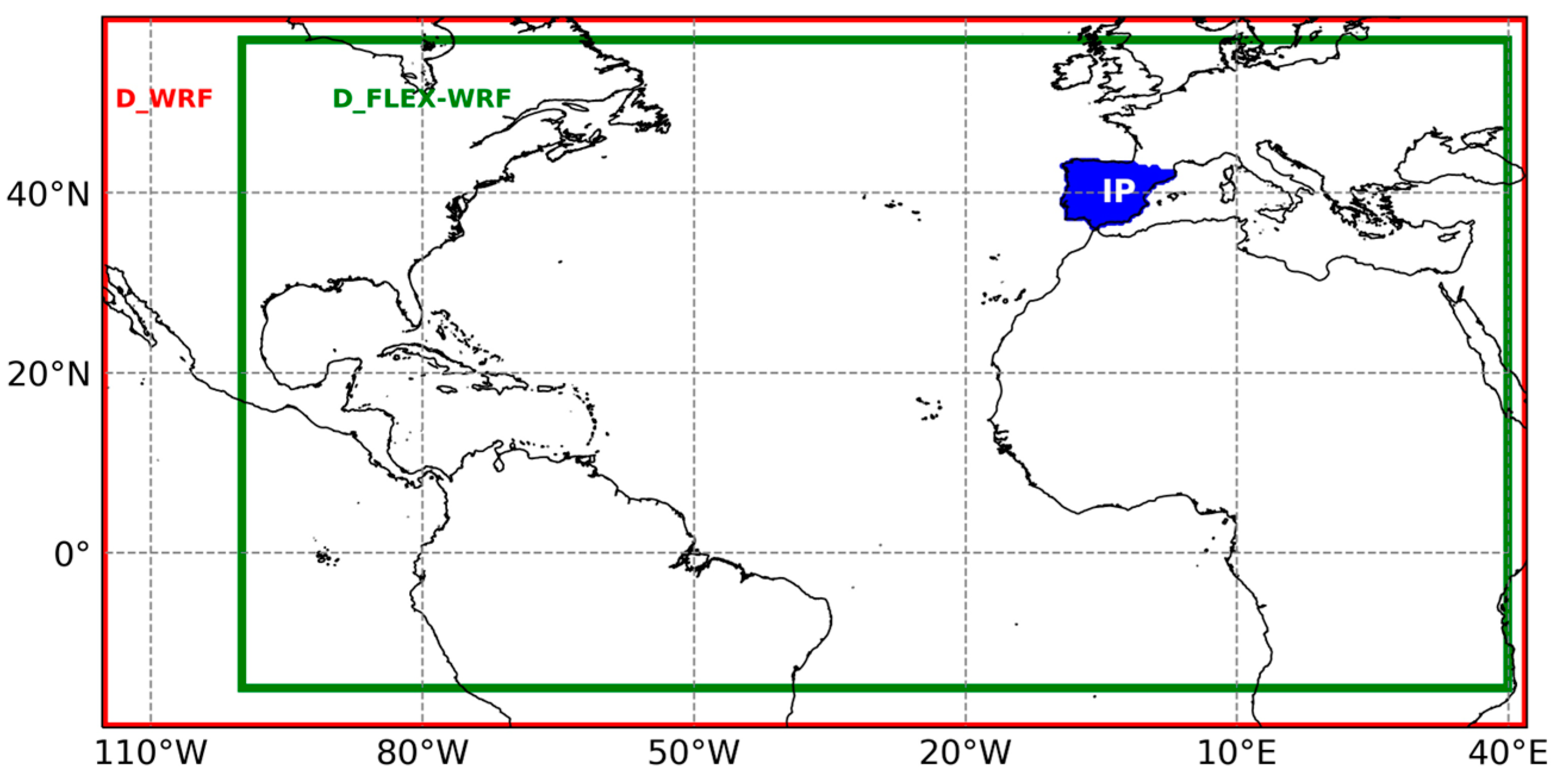
Moreover, the WRF-ERA5 outputs have 40 vertical layers from the surface to 50 hPa with a horizontal spacing of approximately 20 km (480 × 780 nodes), and cover an area of 115.39–42.02° W and 19.41°S–59.51° N (see Figure 1). These parameterization schemes were selected because they have been evaluated and used in several previous investigations involving the same study region [17,20,35]. For the WRF simulations, an initial 1-month spin-up was performed before each simulation. That is, the WRF model is initialized 1-month before for each year to enable the model to adjust from the initial conditions to a state that is consistent with its own numerics and physics and to develop appropriate large-scale circulations [36,37], and to reach a physical equilibrium state following the path defined by the boundary conditions, while forgetting about the initial conditions [38,39,40]. Then, only the outputs for the corresponding year are considered, eliminating the outputs to the simulated month corresponding to the previous year. This approach is carried out to complete a period of 30 years, which is adequate to determine the anomalies of the meteorological fields and the moisture sources for the two summer days of maximum precipitation in the ranking of Ramos et al. [12] mentioned above: 18 September 1999 and 7 September 1989.
2.3. Experimental Setup for FLEXPART-WRF
Once the WRF-ARW simulations were performed, FLEXPART-WRF was used. In this case, for the FLEXPART-WRFv3.2 [19] configuration, Hanna’s scheme [41] was used for turbulence parameterization with the convection scheme activated. This scheme is based on the boundary layer parameters of PBL height, Monin–Obukhov length, convective velocity scale, roughness length, and friction velocity. Skewed rather than Gaussian turbulence was assumed in the convective PBL. The FLEXPART-WRF has 40 levels and 400 × 777 points at which the particles are released in the output grid. The outputs have spatial and temporal resolutions of approximately 20 km and 6 h, respectively. Two million particles are considered in the simulation. A more detailed summary of the configuration and evaluation of the IP is presented by Fernández-Alvarez et al. [20]. The FLEXPART-WRF was run in forward mode during the simulation period for each case study.
2.4. Determination of Moisture Sources
To estimate the moisture sources, the Lagrangian methodology by Stohl and James [14,42] was used to follow the changes in the specific moisture content (q) over time (t, every 6 h) along the backward trajectories described by each atmospheric particle that reached a defined location, calculated using FLEXPART-WRF. The changes in q can be calculated as:
where m is the mass of the particle, and the difference between e and p considers the increase or decrease in the water vapor ratio along the trajectory every 6 h. For this study, the mean residence time of water vapor particles in the atmosphere of approximately 10-days [43,44,45] was considered, which is the maximum time to follow the particles. It should be noted that only precipitating particles are considered. Therefore, these particles, according to Läderach and Sodemann [46], are those in which the specific humidity decreased more than 0.1 g/kg in the 6 h before reaching the target region.
Once the individual (e − p) computations for all precipitated parcels have been calculated, the total surface freshwater flux in each grid cell can be calculated by adding the contributions of all the particles over a grid area (A) at a given time. The total budget is calculated as follows:
where E represents evaporation, P is precipitation, and N is the total number of particles over the grid area (A). Our target region for the study corresponds to the IP (see Figure 1a). It should be noted that a region is considered a moisture source where evaporation dominates over precipitation (E − P > 0) when the backward mode for following the air particles in time is performed [14,42].
In addition, due to moisture losses by precipitation along the particle trajectory, the remote moisture sources will contribute less and less to the final precipitation over the target region [47]. Thus, the fractional contribution of each evaporation location to final precipitation can be estimated as:
where i denotes the particle position at time ti, Q is the specific humidity of the particle when arriving to the target region and Δq′i is the moisture change for each particle. By averaging all the fractional contributions over the grid cell of area A, we computed the moisture source contribution percentage (MSCP) by grid as follows:
where M represents the number of fractional contributions over the grid cell of area A. This method was used to study meteorological systems as in Pérez-Alarcón et al. [48,49] for tropical cyclones. In addition, the TRansport Of water Vapor software (TROVA, [50]) was used for all commented post-processing of the E−P pattern. It was used in the backward in time mode to determine the moisture sources. Finally, the anomalies of the moisture sources were presented, and were determined as the difference in the patterns for each case study day analyzed minus the climatological pattern for that same calendar day over the 30 years (1985–2014; see Section 2.2).
3. Results and Discussion
3.1. Evaluation of the WRF-ARW Configuration Used
The meteorological variables that are used in the following sections to show the synoptic situation of extreme events are evaluated with respect to the ERA5 reanalysis. The variables considered are total precipitation (TP), vertically integrated moisture transport (VIMT), specific humidity at 850 hPa (Q850), total column water (TCW), mean sea level pressure field (MSLP), geopotential height at the 500 hPa level (GPH_500) and geopotential height at the 300 hPa level (GPH_300). For them, the following statistics are considered [51]: Pearson’s correlation (R), Bias (B), Mean Absolute Error (MAE) and Root Mean Square Error (RMSE). In addition, the spatial differences are calculated to show where the WRF-ARW shows a greater bias with respect to the reanalysis. To carry out the evaluation, the WRF-ERA5 variables were interpolated to the ERA5 grid so that they had the same resolution, but the analysis was only performed for the region defined in the WRF domain (see Figure 1). Finally, Table 1 and Table 2 show the results obtained for the extreme events of 18 September 1999 and 7 September 1989, respectively.
In general terms, the WRF-ARW configuration shows good representation with very high R values in the range of 0.8–0.9. However, for the TP the configuration decreases R with a value of ~0.69. In addition, for the variables VIMT, Q850, and MSLP there is a slight underestimation of the pattern and in the rest, there is very little difference, except for TCW where it overestimates the ERA5 by 1.27 kg/m2. Additionally, the MAE shows low values compared to the order of magnitude of each variable. Furthermore, the RSME increases slightly for variables related to moisture transport such as VIMT, Q850, TCW, and total precipitation. This accentuates that in the regions where the maximum values exist, the differences between the simulations and the reanalysis are maximized. Finally, Figure S1 shows the spatial differences for each variable analyzed. It is confirmed that the aforementioned variables are those that present the greatest differences with respect to the ERA5. It should be noted that these differences are accentuated in regions further away from the IP over the Western Atlantic (underestimation) and in mountainous areas such as the Alps and northwest Africa (overestimation).
Moreover, regarding the representation of the variables for the EPE-2 (see Table 2), very similar behavior is observed for R compared to that obtained for EPE-1. However, a slight increase can be seen in the underestimation of the VIMT with a value of −5.25 kg m−1 s −1, for TCW of −0.44 kg/m2, and in the overestimation of total precipitation with 0.33 mm. Additionally, the MAE and RSME statistics reveal very similar values compared to EPE-1, but with slight differences. For example, the RSME for VIMT increases up to 71 kg m−1 s−1, but decreases for TP with a value of ~ 7.30 m, because in this case, there was not such a large area with considerable precipitation values. Regarding the spatial differences for the EPE-2 (Figures S2 and S3), an underestimation is observed for MSLP over the IP and North Africa, but for the variable geopotential height, very little change was obtained. It stands out for this EPE that the WRF-ARW shows slightly displaced areas of intense precipitation (further inland from the IP) for ERA5. In addition, it can be seen that it considerably overestimated the areas with maximum rainfall, influencing notable differences in the southeast of the IP. Finally, an overestimation is observed for the variables VIMT, Q850, and TCW, mostly over the IP but less notable for VIMT. In general, although there are differences in the configuration of the WRF-ARW vs. ERA5, the model shows quite adequate behavior for this type of extreme event in this study region.
3.2. Study Case I: 18 September 1999
3.2.1. Synoptic Situation and Meteorological Variables
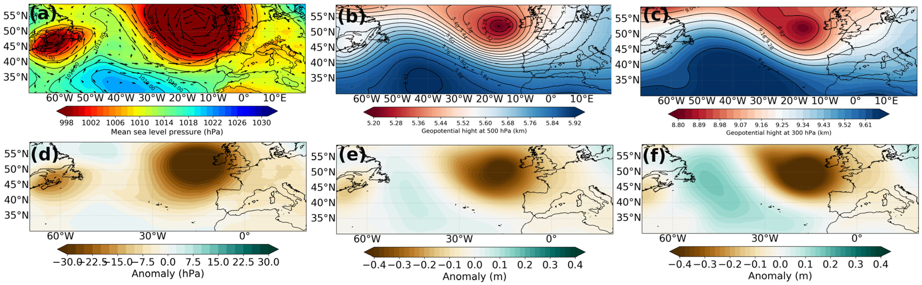
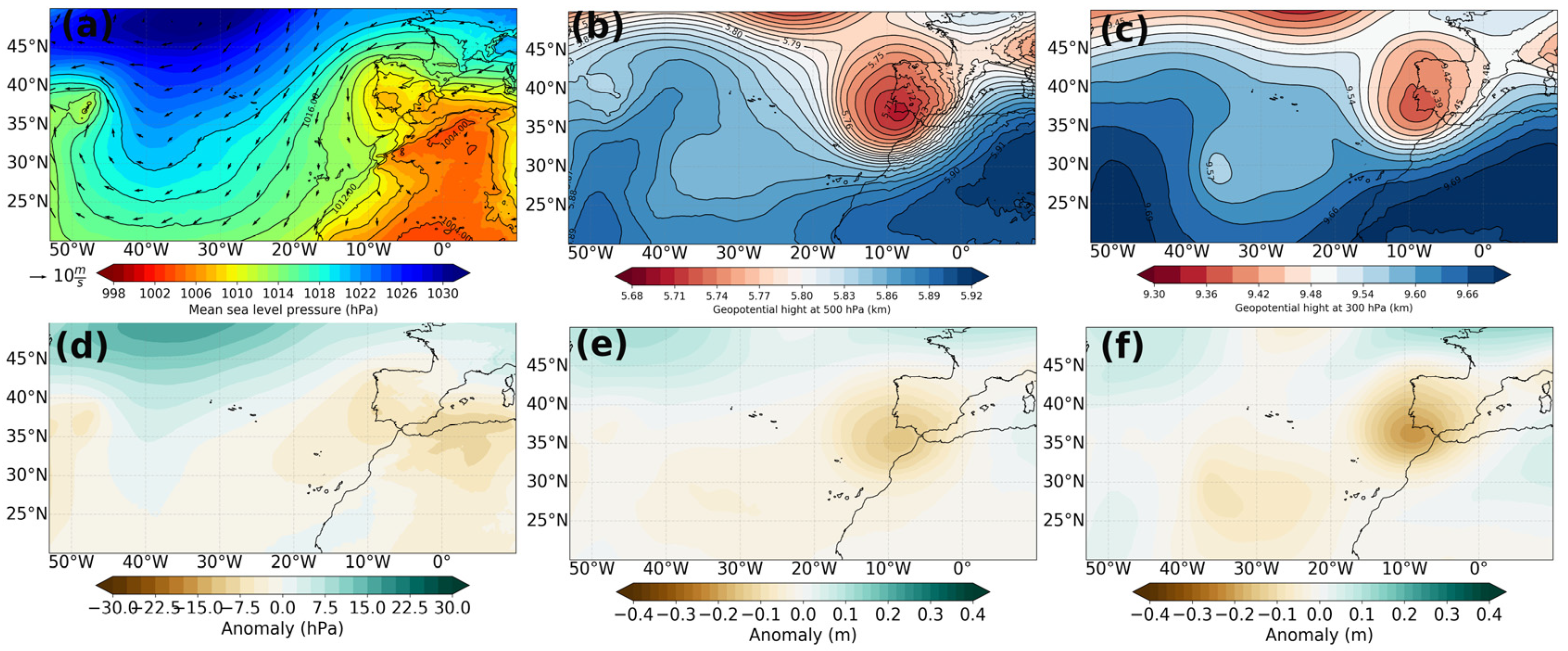
The day 18 September 1999 was marked by the influence of an AR, as shown in Ramos et al. [12]. This AR was associated with the movement of an extratropical cyclone with a well-defined center and mean sea level pressure (MSLP) values of approximately 990 hPa to the west of the British Islands. The system presented a closed circulation with a symmetrical pattern that determined the west–northwest flux from the central North Atlantic to the IP (Figure 2a). Moreover, this extratropical cyclone showed a well-defined structure in the vertical column with a center of low geopotential height values at 500 hPa, equally close to the British Isles however it was slightly displaced meridionally (Figure 2b). In addition, at the 300 hPa level, a weaker center was still observed (Figure 2c). Additionally, it can be seen in Figure 2d–f the anomaly for each field with respect to the mean pattern calculated for the same day over the 30 years. In general, it is observed that anomalous values prevailed both on the surface and in the middle and upper levels of the troposphere with negative anomalies predominantly in the center of the extratropical cyclone.
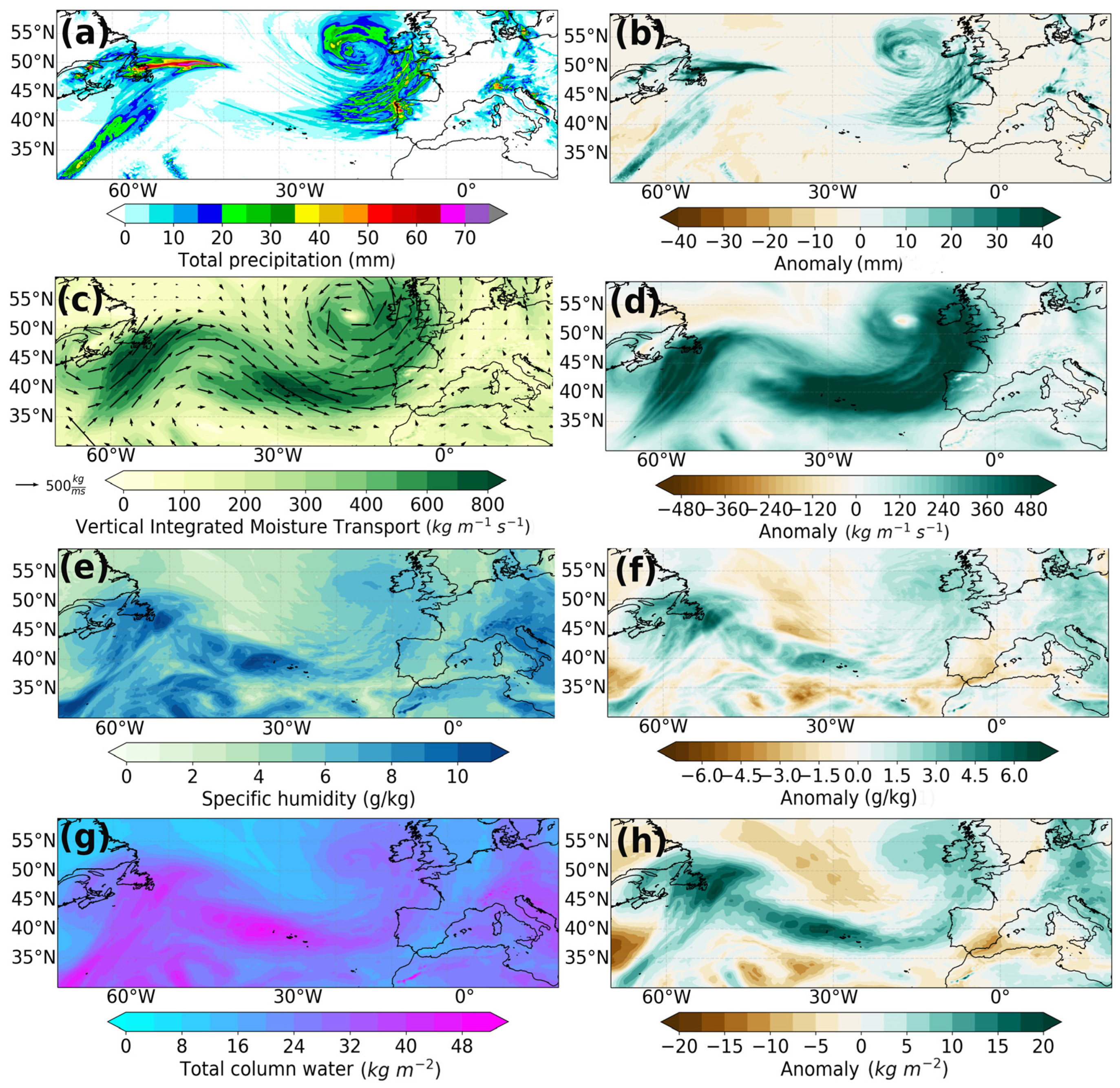
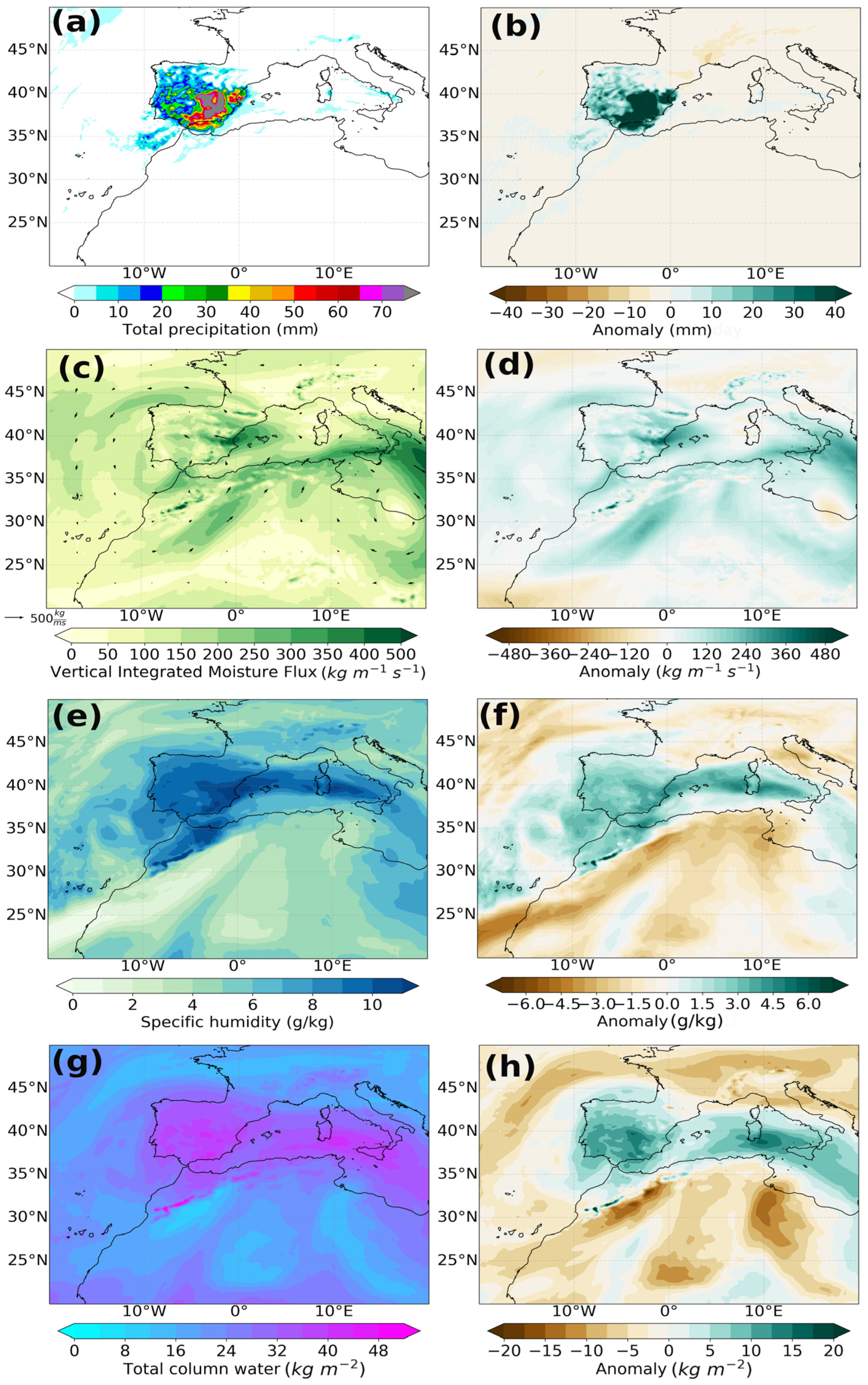
The total precipitation for that day is displayed in Figure 3a. The maximum observed values were recorded in the northwestern region of the IP, with a maximum over Galicia and northern Portugal with approximately 70 mm/day. That day was highlighted by a strong anomaly in the precipitation field in the northwest of the IP and the northeast of the North Atlantic (Figure 3b). These considerable precipitation values may be related to the strong moisture transport (Figure 3c) from the western North Atlantic coast to the IP coast. Strong moisture transport was established by the prevailing atmospheric circulation caused by the extratropical cyclone, resulting in considerable vertical integrated moisture transport (VIMT) values. The VIMT is calculated by vertically integrating moisture fluxes of the u and v components. Specifically, VIMT maxima higher than 800 kg m−1 s−1 were observed in the AR area. Additionally, this determined that on that day, regarding the considered climatological conditions, there was a positive anomaly band that extends from the Western Atlantic to the coasts of Europe (Figure 3d). In addition, at 850 hPa, there was considerable specific moisture content (Figure 3e) across the entire right band of the extratropical cyclone located in the northern area of the IP. In particular, it highlights the maximum specific humidity values over the western and central North Atlantic regions. Similarly, Figure 3g displays the behavior of the total water column on that day. This subfigure shows that the moisture maxima were located in regions on the IP, they were notable up to the center and within areas of the Atlantic. In addition, another low-pressure system was located near the US coast that contributed to the moisture transport. Specifically, very marked positive anomalies were observed for both variables in the regions of maximum VIMT values and negative ones around those regions (Figure 3f,h).
3.2.2. Moisture Sources Causing Precipitation
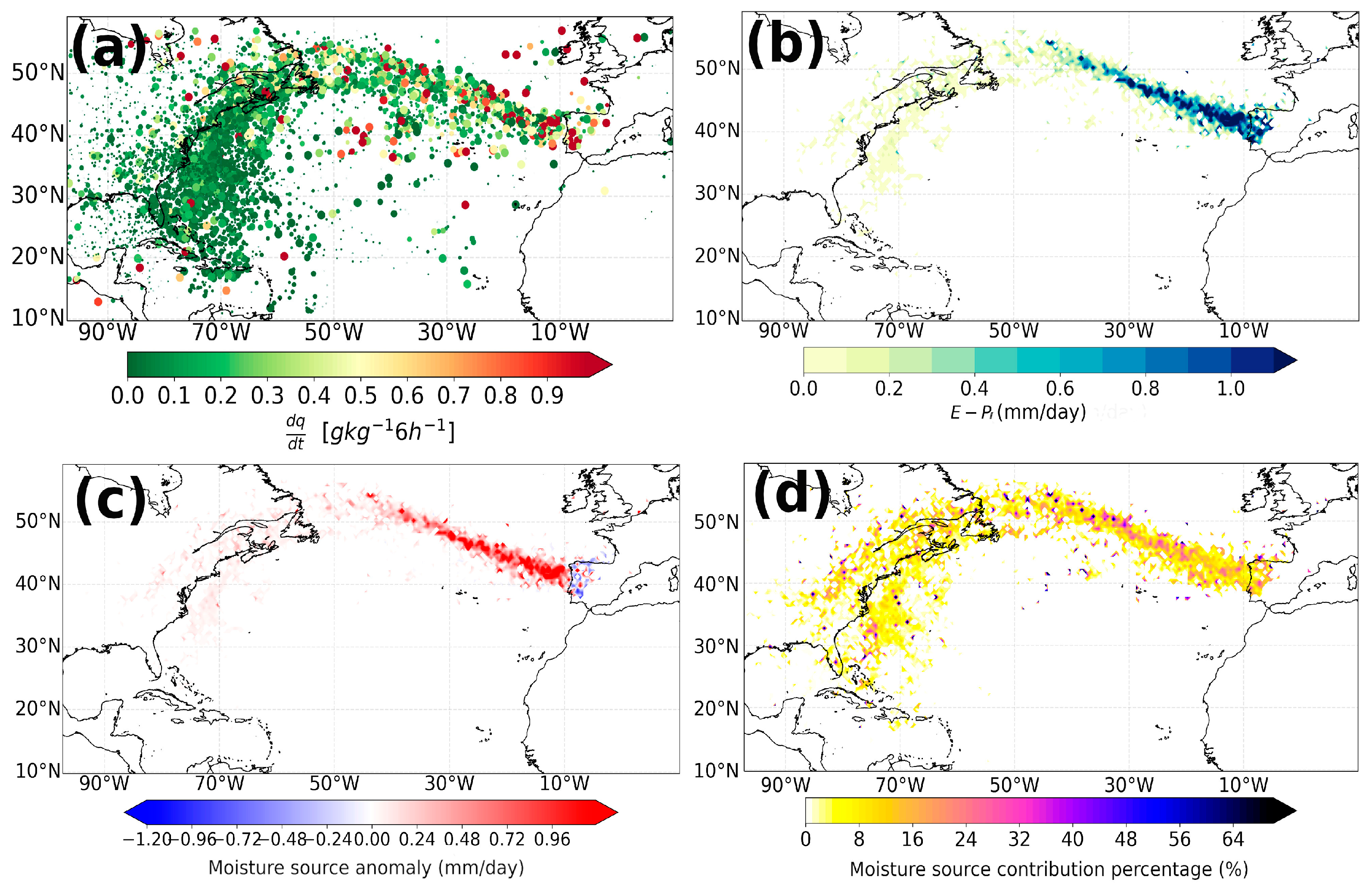
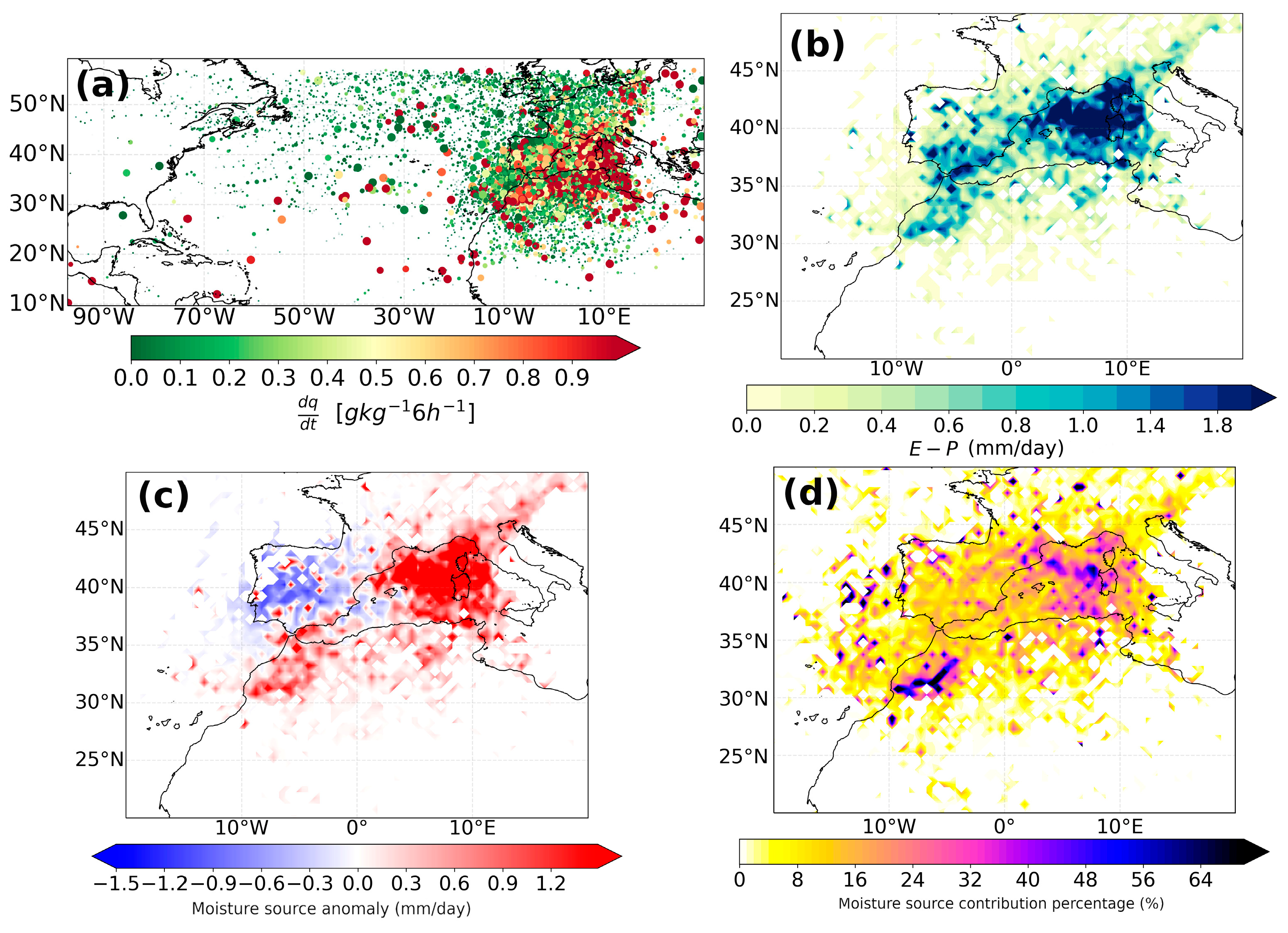
The analysis of moisture sources is presented below. Figure 4a displays the specific humidity changes every 6 h for the trajectories of a sample of particles that generated precipitation in the target region (IP). In this case, the size of the circle shows the magnitude of the humidity change in 6 h. Therefore, the regions where the particles had the greatest moisture uptake corresponded to the center and east of the North Atlantic between 10–50° W and 40–50° N (0.4–0.9 g kg−1 6 h−1). In addition, an increase was observed mainly in the northern Caribbean Sea and near the coasts of the United States, however to a lesser extent, with values up to 0.3 g kg−1 6 h−1. Finally, it was observed that for more distant regions, there was a lower contribution of moisture from particles that precipitated over the IP.
Figure S4 presents the spatial representation for the 10 days backward in time for a sample of particle trajectories as a function of height. They are distributed vertically and reach heights equal to or greater than 10 km. It was also observed that over the Caribbean Sea and Western Atlantic, the height values were lower, however as they increased in latitude, they reached higher heights. This could be associated with the prevailing atmospheric circulation in this synoptic situation, delimited by the strong extratropical cyclone that moved over the Atlantic during that period. Furthermore, this behavior detailed day-by-day is shown in Figures S5–S7.
Figure 4b displays the source regions that generated precipitation over the target region (IP) according to the method of Läderach and Sodemann [46] considering the threshold proposed in Section 2.4. The moisture sources were observed closer to the IP, located mainly in a band between 40–50° N, with a decreasing contribution from the remote sources as the source was far from the IP (Western Atlantic). However, it was verified that, on this day, there was mostly a positive anomaly for moisture uptake (Figure 4c) regarding the climatological pattern over 30 years. Therefore, the values for the moisture sources were higher than the historical pattern, reaching a maximum in areas close to the IP. It should be noted that the previously mentioned pattern was distributed in an elongated shape, increasing in width near the IP and the humidity around the IP.
The moisture source pattern for 18 September 1999 differed from the climatological pattern of sources presented by Ramos et al. [52]. These authors demonstrated that the average moisture source pattern for ARs that reached the IP were located at 20–40° N. However, a latitudinal shift was observed in our case study. Figure 4d displays the moisture source contribution percentages in this study. Remote moisture sources contribute less to the final moisture content that reaches the target region [47]. The maximum percentages were located east of the 50° W meridian (8–32%); however, to the west, the values tended to be less than 8%. Finally, the difference between the contribution patterns of the sources was not considered relevant for this case study.
3.3. Study Case II: 7 September 1989
3.3.1. Synoptic Situation and Meteorological Variables
The second EPE case study (7 September 1989) corresponded to a cut-off low system (COL) that affected the IP from 4 September 1989 [21,22], with maximum values of precipitation over the IP on 7 September 1989 [12]. The meteorological system is located near Cabo San Vicente, Portugal (Figure 5a). The system had a well-defined structure with the typical characteristics of a COL [22] at mid- and high-levels of the troposphere (Figure 5b,c) but without a sign at the surface (where a trough and ridge pattern can be seen in Figure 5a), as in Molina [21]. Therefore, at 300 hPa (Figure 5c), a region of low values of geopotential height was observed (central minimum of approximately 9 km) with very closed circulation around the southwest of the IP. At 500 hPa, it showed a less intense pattern, however, it maintained a very well-defined closed circulation and a prevailing strong subtropical anticyclonic ridge (Figure 5b). The three fields analyzed both on the surface and in the levels of the troposphere showed negative anomalies, showing that that day differed from the climatic pattern, dominated by low-pressure systems (Figure 5d–f). Finally, a strong geopotential gradient to the south-southeast of the COL was observed over southeastern region of Spain and the Levante region [21]. It should be noted that strong storms, associated with a strong suction exerted by the air from low levels, were recorded in this region causing the formation of large cloudy areas [21,22].
Figure 6a displays the precipitation pattern in the COL of 7 September 1989. The maximum values were observed in the southeastern IP and were higher than 80 mm in regions closer to the coast. It can be affirmed that the values for that day in those areas were anomalous (>40 mm, Figure 6b) and higher than the climatological average for that day in the 1985–2014 period. On this day, the VIMT came mainly from North Africa, the Strait of Gibraltar, and the western Mediterranean Sea, conditioned by the circulation in height (Figure 6c). This determined positive VIMT anomalies in the northeast region of the IP and North Africa. It is noted that these values are not comparable with the anomaly obtained for this variable in the EPE-1 (Figure 6d). In addition, there was high moisture content at 850 hPa, with maximum values in the Mediterranean (Figure 6e). These conditions, in addition to the strong convergence of the moisture flux, favored the formation of strong storms (Figure S8). Additionally, high values of the total column water (Figure 6g) were observed, providing favorable conditions for heavy rainfall to be generated in this region owing to the existence of cold air at higher levels, which allowed the condensation of water vapor carried by the updrafts. Finally, the aforementioned is verified with the positive anomaly values, since that day there was a notable moisture layer at 850 hPa and a water content integrated in the vertical (Figure 6f,h) that extended from the Mediterranean Sea to the IP, covering most of it.
3.3.2. Moisture Sources Causing Precipitation
The precipitation generated by COLs is the result of a strong convergence of moisture flux at the local scale and, to a lesser extent, moisture transport from remote sources [22]. This can be observed in Figure 7a, which displayed the moisture changes in the positions of the particles used in tracking. Although particles with humidity from more remote sources to the IP, the maximum changes in humidity were achieved in North Africa and west of the Mediterranean Sea, near the system center.
Figure S9 shows the trajectories as a function of height for a sample of particles. They were mainly distributed from the surface to medium levels, which may be associated with the presence of cold air in the upper layers of the atmosphere. This determines the condensation of all the moisture displaced by the updrafts. This behavior was observed in the vertical distribution of particles per day (Figures S10–S12). In addition, the accumulation of particles was observed vertically for days 1–3 backward in time, as determined by the convergence of the moisture flux (Figure S8) associated with the COL.
Figure 7b displays the moisture sources (method described in Section 2.4) for the COL under study. The most important source region for this extreme precipitation event was the western Mediterranean (Figure 7b). The Mediterranean Sea constitutes a fundamental moisture source with an important contribution to events of this type that develop in the area [17,53]. In addition, it was observed that part of the moisture from the precipitating particles originated in the central and eastern regions of the IP, with the southeastern region of the IP where the maximum continental moisture was taken up. This is related to the typical recycling processes (the fraction of the target precipitation that has evaporated in the target domain itself during the previous 10 days [14] along the IP during summer [1]. Another source region, albeit to a lesser extent, was North Africa and the Strait of Gibraltar.
A high anomaly was observed for moisture uptake in the 30-year climatology pattern in the Western Mediterranean Sea and North African regions. However, the moisture sources on the IP showed a negative anomaly in most of the IP. Finally, Figure 7d shows the contribution of the moisture source. A similar percentage was observed in the entire area analyzed, except for the western Mediterranean and northwestern Africa, where there are values above 40%. Therefore, the contribution of the western Mediterranean to the generation of heavy rainfall on 7 September 1989 stands out.
4. Conclusions
This study analyzed the moisture sources for the two major extreme precipitation events (EPEs) during summer in the period of 1950–2008 on the IP. These events were an atmospheric river (AR) that occurred on 18 September 1999 and a cutoff low (COL) system that occurred on 7 September 1989. For characterization, a dynamic downscaling methodology was used with the WRF-ARW regional model and FLEXPART-WRF dispersion model. The data used as the initial and boundary conditions belonged to the ERA5 reanalysis. To calculate the moisture source pattern, a Lagrangian methodology [14,42] was used, considering only the precipitating particles involved in each system [47]. In addition, a detailed analysis of the meteorological fields associated with moisture transport patterns is presented.
In the first case study, the AR, considerable moisture transport associated with an extratropical cyclone located to the east in the North Atlantic, was observed on 18 September 1999. In addition, an important vertically integrated moisture content allowed the generation of precipitation. Specifically, the moisture sources were located mainly between 40–50° N, with remote sources located in the western Atlantic being less important. This behavior was corroborated by the maximum percentages of moisture contribution that reached the IP, which were a maximum east of the 50° W meridian (8–32%) and less than 8% west of this position. Finally, the moisture source pattern presented an anomaly with respect to the climatological pattern with a latitudinal shift.
In the COL case, intense rainfall was observed, especially southeast of the IP because there was significant moisture transport associated and strong convergence of the moisture flux around the IP. In addition, a high moisture content was observed at a pressure level of 850 hPa. Regarding the origin of the moisture sources, it was found that the most important source region of this extreme precipitation event was the western Mediterranean. This was demonstrated by the values for the contribution of moisture sources being greater than 40% in this area and a strong anomaly in the climatological pattern. The precipitation recycling processes with maximum values were observed in the southeastern region of the IP (approximately 16%). Other regions of origin, however to a lesser extent, were North Africa and the Strait of Gibraltar, with contributions of approximately 16% to the moisture supply to this event.
In conclusion, the extreme events, although they occurred in the month of September, the meteorological systems that originate them are physically different, therefore their moisture sources differ remarkably. In other words, EPE-1 originated from a very well-structured extratropical cycle that was associated with an AR. This AR generated strong moisture transport from remote source regions [54] associated with the presence of a notable moisture content. These conditions shown by positive anomalous values for these variables determined a favorable scenario for the extreme precipitation event. However, EPE-2 originated from the presence of a very well structured low cut-off system at medium and high levels that, together with an anomalous layer of humidity in practically the entire vertical column, determined a strong convergence of the humidity flow southeast of the IP.
Finally, in future research, we intend to conduct a study on moisture sources with a greater number of extreme precipitation events in the summer for the IP. In addition, to updating the ranking of events up to the present, the events of previous decades were compared with those of the current decades.
Supplementary Materials
The following supporting information can be downloaded at: https://www.mdpi.com/article/10.3390/atmos14081213/s1, Figure S1: Comparison of the meteorological fields obtained with WRF forced with ERA5 (left column) with respect to the ERA5 reanalysis (middle column). In the right column the differences of the WRF-ERA5 minus ERA5 are shown. The fields from top to bottom are: mean sea level pressure field (MSLP), geopotential height at the 500 hPa level, geopotential height at the 300 hPa level, total precipitation, vertically integrated moisture transport, specific humidity at 850 hPa and total column water. Study case: 18 September 1999; Figure S2: Comparison of the meteorological fields obtained with WRF forced with ERA5 (left column) with respect to the ERA5 reanalysis (middle column). In the right column the differences of the WRF-ERA5 minus ERA5 are shown. The fields from top to bottom are: mean sea level pressure field (MSLP), geopotential height at the 500 hPa level and geopotential height at the 300 hPa level. Study case: 7 September 1989; Figure S3: Comparison of the meteorological fields obtained with WRF forced with ERA5 (left column) with respect to the ERA5 reanalysis (middle column). In the right column the differences of the WRF-ERA5 minus ERA5 are shown. The fields from top to bottom are: total precipitation, vertically integrated moisture transport, specific humidity at 850 hPa and total column water. Study case: 7 September 1989; Figure S4: Representation of the trajectories for a sample of particles that reach the IP on 18 September 1999; Figure S5: Representation of the spatial and vertical distribution of a sample of particles that reached the IP on 18 September 1999. The subfigures correspond to days 7, 8, 9 and 10 backward in time; Figure S6: Representation of the spatial and vertical distribution of a sample of particles that reached the IP on 18 September 1999. The subfigures correspond to days 3, 4, 5 and 6 backward in time; Figure S7: Representation of the spatial and vertical distribution of a sample of particles that reached the IP on 18 September 1999. The subfigures correspond to days 1 and 2 backward in time; Figure S8: Moisture flux divergence for September 7, 1989 in mm day−1; Figure S9: Representation of the trajectories for a sample of particles that reach the IP on 7 September 1989; Figure S10: Representation of the spatial and vertical distribution of a sample of particles that reached the IP on 7 September 1989. The subfigures correspond to days 7, 8, 9 and 10 backward in time; Figure S11: Representation of the spatial and vertical distribution of a sample of particles that reached the IP on 7 September 1989. The subfigures correspond to days 3, 4, 5 and 6 backward in time; Figure S12: Representation of the spatial and vertical distribution of a sample of particles that reached the IP on 7 September 1989. The subfigures correspond to days 1 and 2 backward in time.
Author Contributions
G.A.-S., J.C.F.-A. and R.N. conceived the idea of the study. G.A.-S. and J.C.F.-A. processed the data and created the figures. G.A.-S., J.C.F.-A. and R.N. analyzed the results and wrote the manuscript. All authors analyzed the results and revised the manuscript. All authors have read and agreed to the published version of the manuscript.
Funding
This work is supported by the SETESTRELO project (PID2021-122314OB-I00) funded by the Ministerio de Ciencia, Innovación y Universidades, Spain. Partial support was also obtained from the Xunta de Galicia under the project “Programa de Consolidación e Estructuración de Unidades de Investigación Competitivas (Grupos de Referencia Competitiva)” (ED431C 2021/44).
Data Availability Statement
Simulations with WRF-ARW and FLEXPART-WRF and codes can be obtained by correspondence with the authors.
Acknowledgments
G.A.-S. acknowledge the support from Consejo Superior de Investigaciones Científicas under the grant JAE Intro 2022 (grant no. JAEINT_22_02769). J.C.F.-A. acknowledge the support from the Xunta de Galicia under the grant no. ED481A-2020/193. G.A.-S., J.C.F.-A. and R.N. thank Luis Gimeno for her help in the development of the research. In addition, this work has been made possible thanks to the computing resources and technical support provided by CESGA (Centro de Supercomputación de Galicia) and Red Española de Supercomputación (RES) (AECT-2022-3-0009 and DATA-2021-1-0005).
Conflicts of Interest
The authors declare no conflict of interest.
References
- Gimeno, L.; Stohl, A.; Trigo, R.M.; Dominguez, F.; Yoshimura, K.; Yu, L.; Drumond, A.; Durán-Quesada, A.M.; Nieto, R. Oceanic and terrestrial sources of continental precipitation. Rev. Geophys. 2012, 50, RG4003. [Google Scholar] [CrossRef] [Green Version]
- Gimeno, L.; Nieto, R.; Trigo, R.; Vicente-Serrano, S.M.; López-Moreno, J.I. Where does the Iberian Peninsula moisture come from? An answer based on a Lagrangian approach. J. Hydrometeorol. 2010, 11, 421–436. [Google Scholar] [CrossRef] [Green Version]
- Rios-Entenza, A.; Miguez-Macho, G. Moisture recycling and the maximum of precipitation in spring in the Iberian Peninsula. Clim. Dyn. 2014, 42, 3207–3231. [Google Scholar] [CrossRef]
- Rios-Entenza, A.; Soares, P.M.; Trigo, R.M.; Cardoso, R.M.; Miguez-Macho, G. Moisture recycling in the Iberian Peninsula from a regional climate simulation: Spatiotemporal analysis and impact on the precipitation regime. J. Geophys. Res. Atmos. 2014, 119, 5895–5912. [Google Scholar] [CrossRef] [Green Version]
- Lionello, P. The Climate of the Mediterranean Region: From the Past to the Future; Elsevier: Amsterdam, The Netherlands, 2012. [Google Scholar]
- Trigo, R.M.; Valente, M.A.; Trigo, I.F.; Miranda, P.M.A.; Ramos, A.M.; Paredes, D.; García-Herrera, R. The impact of North Atlantic wind and cyclone trends on european precipitation and significant wave height in the atlantic, trends and directions in climate research. Ann. N. Y. Acad. Sci. 2008, 1146, 212–234. [Google Scholar] [CrossRef] [Green Version]
- Pereira, S.; Ramos, A.M.; Zêzere, J.L.; Trigo, R.M.; Vaquero, J.M. Spatial impact and triggering conditions of the exceptional hydrogeomorphological event of December 1909 in Iberia. Nat. Hazards Earth Syst. Sci. 2016, 16, 371–390. [Google Scholar] [CrossRef] [Green Version]
- Trigo, R.M.; Ramos, C.; Pereira, S.S.; Ramos, A.M.; Zêzere, J.L.; Liberato, M.L.R. The deadliest storm of the 20th century striking Portugal; flood impacts and atmospheric circulation. J. Hydrol. 2016, 541, 597–610. [Google Scholar] [CrossRef]
- García-Herrera, R.; Barriopedro, D.; Hernández, E.; Paredes, D.; Correoso, J.F.; Prieto, L. The 2001 mesoscale convective systems over Iberia and the Balearic Islands. Meteorol. Atmos. Phys. 2005, 90, 225–243. [Google Scholar] [CrossRef]
- Paredes, D.; Trigo, R.M.; García-Herrera, R.; Trigo, I.F. Understanding precipitation changes in Iberia in early spring: Weather typing and storm-tracking approaches. J. Hydrometeorol. 2006, 7, 101–113. [Google Scholar] [CrossRef] [Green Version]
- de Luis, M.; Brunetti, M.; Gonzalez-Hidalgo, J.C.; Longares, L.A.; Martin-Vide, J. Changes in seasonal precipitation in the Iberian Peninsula during 1946–2005. Glob. Planet. Chang. 2010, 74, 27–33. [Google Scholar] [CrossRef]
- Ramos, A.M.; Martins, M.J.; Tomé, R.; Trigo, R.M. Extreme precipitation events in summer in the Iberian Peninsula and its relationship with atmospheric rivers. Front. Earth Sci. 2018, 6, 110. [Google Scholar]
- Keune, J.; Schumacher, D.L.; Miralles, D.G. A unified framework to estimate the origins of atmospheric moisture and heat using Lagrangian models. Geosci. Model Dev. 2022, 15, 1875–1898. [Google Scholar] [CrossRef]
- Stohl, A.; James, P. A Lagrangian analysis of the atmospheric branch of the global water cycle. Part I: Method description, validation, and demonstration for the August 2002 flooding in central Europe. J. Hydrometeorol. 2004, 5, 656–678. [Google Scholar] [CrossRef]
- Stohl, A. Computation, accuracy and applications of trajectories—A review and bibliography. Atmos. Environ. 1998, 32, 947–966. [Google Scholar] [CrossRef]
- Ramos, A.M.; Trigo, R.M.; Liberato, M.L.R. A ranking of high resolution daily precipitation extreme events for the Iberian Peninsula. Atmos. Sci. Lett. 2014, 15, 328–334. [Google Scholar] [CrossRef]
- Insua-Costa, D.; Miguez-Macho, G.; Llasat, M.C. Local and remote moisture sources for extreme precipitation: A study of the two catastrophic 1982 western Mediterranean episodes. Hydrol. Earth Syst. Sci. 2019, 23, 3885–3900. [Google Scholar] [CrossRef] [Green Version]
- Cloux, S.; Garaboa-Paz, D.; Insua-Costa, D.; Miguez-Macho, G.; Pérez-Muñuzuri, V. Extreme precipitation events in the Mediterranean area: Contrasting two different models for moisture source identification. Earth Syst. Sci. 2021, 25, 6465–6477. [Google Scholar] [CrossRef]
- Brioude, J.; Arnold, D.; Stohl, A.; Cassiani, M.; Morton, D.; Seibert, P.; Angevine, W.; Evan, S.; Dingwell, A.; Fast, J.D.; et al. The lagrangian particle dispersion model flexpart-wrf version 3.1. Geosci. Model Dev. 2013, 6, 1889–1904. [Google Scholar] [CrossRef] [Green Version]
- Fernández-Alvarez, J.C.; Vázquez, M.; Pérez-Alarcón, A.; Nieto, R.; Gimeno, L. Comparison of Moisture Sources and Sinks Estimated with Different Versions of FLEXPART and FLEXPART-WRF Models Forced with ECMWF Reanalysis Data. J. Hydrometeorol. 2023, 24, 221–239. [Google Scholar] [CrossRef]
- Molina, J.J.C. Convección profunda sobre el Mediterráneo español: Lluvias torrenciales durante los días 4 al 7 de septiembre de 1989 en Andalucía oriental, Murcia, Levante, Cataluña y Mallorca. Paralelo 1989, 37, 51–80. [Google Scholar]
- Nieto, R.; Gimeno, L.; de la Torre, L.; Ribera, P.; Gallego, D.; García-Herrera, R.; García, J.A.; Nuñez, M.; Redaño, A.; Lorente, J. Climatological features of cutoff low systems in the Northern Hemisphere. J. Clim. 2005, 18, 3085–3103. [Google Scholar] [CrossRef] [Green Version]
- Nieto, R.; Gimeno, L.; Añel, J.A.; de la Torre, L.; Gallego, D.; Barriopedro, D.; Gallego, M.C.; Gordillo, A.; Redaño, A.; Delgado, G. Analysis of the precipitation and cloudiness associated with COLs occurrence in the Iberian Peninsula. Meteorol. Atmos. Phys. 2007, 96, 103–119. [Google Scholar] [CrossRef]
- Efemerides AEMET. Available online: https://www.aemet.es/es/serviciosclimaticos/datosclimatologicos/efemerides_sucesos*?dateDia=6&dateMes=8&dateAnyo=1989&palabra=Introduzca+texto (accessed on 10 March 2023).
- Hersbach, H.; Bell, B.; Berrisford, P.; Hirahara, S.; Horányi, A.; Muñoz-Sabater, J.; Nicolas, J.; Peubey, C.; Radu, R.; Schepers, D.; et al. The ERA5 global reanalysis. Q. J. R. Meteorol. Soc. 2020, 146, 1999–2049. [Google Scholar] [CrossRef]
- Skamarock, W.C.; Klemp, J.B.; Dudhia, J.; Gill, D.O.; Barker, D.M.; Duda, M.G.; Huang, X.Y.; Wang, W.; Powers, J.G. Description of the Advanced Research WRF Version 3; Technical Report; National Center for Atmospheric Research: Boulder, CO, USA, 2008. [Google Scholar]
- Fernández-Alvarez, J.C.; Pérez-Alarcón, A.; Eiras-Barca, J.; Ramos, A.M.; Rahimi-Esfarjani, S.; Nieto, R.; Gimeno, L. Changes in moisture sources of atmospheric rivers landfalling the Iberian Peninsula with WRF-FLEXPART. J. Geophys. Res. Atmos. 2023, 128, e2022JD037612. [Google Scholar] [CrossRef]
- Hong, S.Y.; Lim, J.O.J. The WRF single-moment 6-class microphysics scheme (WSM6). J. Korean Meteorol. Soc. 2006, 42, 129–151. [Google Scholar]
- Hong, S.Y.; Noh, Y.; Dudhia, J. A new vertical diffusion package with an explicit treatment of entrainment processes. Mon. Weather Rev. 2006, 134, 2318–2341. [Google Scholar] [CrossRef] [Green Version]
- Jimenez, P.A.; Dudhia, J.; Gonzalez-Rouco, J.F.; Navarro, J.; Montavez, J.P.; Garcia–Bustamante, E. A revised scheme for the WRF surface layer formulation. Mon. Weather Rev. 2012, 140, 898–918. [Google Scholar] [CrossRef] [Green Version]
- Tewari, M.; Chen, F.; Wang, W.; Dudhia, J.; LeMone, M.; Mitchell, K.; Ek, M.; Gayno, G.; Wegiel, J.; Cuenca, R.H. Implementation and verification of the unified Noah land surface model in the WRF model. In Proceedings of the 20th Conference on Weather Analysis and Forecasting/16th Conference on Numerical Weather Prediction, Seattle, WA, USA, 12–16 January 2004. [Google Scholar]
- Iacono, M.J.; Delamere, J.S.; Mlawer, E.J.; Shephard, M.W.; Clough, S.A.; Collins, W.D. Radiative forcing by long-lived greenhouse gases: Calculations with the AER radiative transfer models. J. Geophys. Res. Atmos. 2008, 113, D13103. [Google Scholar] [CrossRef]
- Kain, J.S. The Kain–Fritsch Convective Parameterization: An Update. J. Appl. Meteorol. 2004, 43, 170–181. [Google Scholar]
- Miguez-Macho, G.; Stenchikov, G.L.; Robock, A. Spectral nudging to eliminate the effects of domain position and geometry in regional climate model simulations. J. Geophys. Res. Atmos. 2004, 109, D13104. [Google Scholar] [CrossRef] [Green Version]
- Insua-Castro, D.; Miguez-Macho, G. A new moisture tagging capability in the Weather Research and Forecasting model: Formulation, validation and application to the 2014 Great Lake-effect snowstorm. Earth Syst. Dyn. 2018, 9, 167–185. [Google Scholar] [CrossRef] [Green Version]
- Jankov, I.; Gallus, W.A., Jr.; Segal, M.; Koch, S.E. Influence of initial conditions on the WRF–ARW model QPF response to physical parameterization changes. Weather. Forecast. 2007, 22, 501–519. [Google Scholar] [CrossRef] [Green Version]
- Skamarock, W.C.; Klemp, J.B. A time-split nonhydrostatic atmospheric model for weather research and forecasting applications. J. Comput. Phys. 2008, 227, 3465–3485. [Google Scholar] [CrossRef]
- Yang, Z.L.; Dickinson, R.E.; Henderson-Sellers, A.; Pitman, A.J. Preliminary study of spin-up processes in land surface models with the first stage data of Project for Intercomparison of Land Surface Parameterization Schemes Phase 1(a). J. Geophys. Res. Atmos. 1995, 100, 16553–16578. [Google Scholar] [CrossRef]
- Giorgi, F.; Mearns, L.O. Introduction to special section: Regional climate modeling revisited. J. Geophys. Res. Atmos. 1999, 104, 6335–6352. [Google Scholar] [CrossRef]
- Denis, B.; Laprise, R.; Caya, D.; Côté, J. Downscaling ability of one-way nested regional climate models: The Big-Brother Experiment. Clim. Dyn. 2002, 18, 627–646. [Google Scholar]
- Hanna, S.R. Applications in air pollution modelling. In Atmospheric Turbulence and Air Pollution Modelling; Reidel Publishing Company: Dordrecht, The Netherlands, 1982; pp. 275–310. [Google Scholar]
- Stohl, A.; James, P.A. A Lagrangian analysis of the atmospheric branch of the global water cycle: Part II: Earth’s river catchments ocean basins, and moisture transports between them. J. Hydrometeorol. 2005, 6, 961–984. [Google Scholar] [CrossRef]
- Numaguti, A. Origin and recycling processes of precipitating water over the Eurasian continent: Experiments using an atmospheric general circulation model. J. Geophys. Res. 1999, 104, 1957–1972. [Google Scholar] [CrossRef]
- van der Ent, R.J.; Tuinenburg, O. A The residence time of water in the atmosphere revisited. Hydrol. Earth Syst. Sci. 2017, 21, 779–790. [Google Scholar] [CrossRef] [Green Version]
- Gimeno, L.; Eiras-Barca, J.; Durán-Quesada, A.M.; Dominguez, F.; van der Ent, R.; Sodemann, H.; Sánchez-Murillo, R.; Nieto, R.; Kirchner, J.W. The residence time of water vapour in the atmosphere. Nat. Rev. Earth Environ. 2021, 2, 558–569. [Google Scholar] [CrossRef]
- Läderach, A.; Sodemann, H. A revised picture of the atmospheric moisture residence time. Geophys. Res. Lett. 2016, 43, 924–933. [Google Scholar] [CrossRef] [Green Version]
- Sodemann, H.; Schwierz, C.; Wernli, H. Interannual variability of Greenland winter precipitation sources: Lagrangian moisture diagnostic and North Atlantic Oscillation influence. J. Geophys. Res. Atmos. 2008, 113, D03107. [Google Scholar] [CrossRef] [Green Version]
- Pérez-Alarcón, A.; Sorí, R.; Fernández-Alvarez, J.C.; Nieto, R.; Gimeno, L. Where does the moisture for North Atlantic tropical cyclones come from? J. Hydrometeorol. 2022, 23, 457–472. [Google Scholar] [CrossRef]
- Pérez-Alarcón, A.; Fernández-Alvarez, J.C.; Sorí, R.; Nieto, R.; Gimeno, L. Moisture source identification for precipitation associated with tropical cyclone development over the Indian Ocean: A Lagrangian approach. Clim. Dyn. 2022, 60, 2735–2758. [Google Scholar] [CrossRef]
- Fernández-Alvarez, J.C.; Pérez-Alarcón, A.; Nieto, R.; Gimeno, L. TROVA: TRansport Of water VApor. SoftwareX 2022, 20, 101228. [Google Scholar] [CrossRef]
- Forecast Verification—Issues, Methods and FAQ. Forecast Verification—Methods and FAQ. Available online: https://www.cawcr.gov.au/ (accessed on 30 April 2023).
- Ramos, A.M.; Nieto, R.; Tomé, R.; Gimeno, L.; Trigo, R.M.; Liberato, M.L.; Lavers, D.A. Atmospheric rivers moisture sources from a Lagrangian perspective. Earth Syst. Dyn. 2016, 7, 371–384. [Google Scholar] [CrossRef] [Green Version]
- Nieto, R.; Gimeno, L.; Drumond, A.; Hernandez, E. A Lagrangian identification of the main moisture sources and sinks affecting the Mediterranean area. WSEAS Trans. Environ. Dev. 2010, 6, 365–374. [Google Scholar]
- Gimeno, L.; Nieto, R.; Vázquez, M.; Lavers, D.A. Atmospheric Rivers: A mini-review. Front. Earth Sci. 2014, 2, 2. [Google Scholar] [CrossRef]
Figure 1.
Domains used for WRF-ARW (red) and FLEXPART-WRF (green) in the simulations. Target region (blue) considered for particle tracking.
Figure 1.
Domains used for WRF-ARW (red) and FLEXPART-WRF (green) in the simulations. Target region (blue) considered for particle tracking.

Figure 2.
September 18, 1999: Meteorological fields (top row) obtained with the outputs of WRF-ARW forced with ERA5 reanalysis data: (a) mean sea level pressure field (MSLP), (b) geopotential height at the 500 hPa level and (c) geopotential height at the 300 hPa level. Anomaly (d–f), bottom row) for each field with respect to the mean pattern calculated for the same day over 30 years.

Figure 3.
September 18, 1999: Meteorological fields (left column) obtained with the outputs of WRF-ARW forced with ERA5 reanalysis data: (a) total precipitation, (c) vertically integrated moisture transport, (e) specific humidity at 850 hPa and (g) total column water. Anomaly for each field ((b,d,f,h), right column) with respect to the mean pattern calculated for the same day over 30 years.

Figure 4.
Analysis of moisture sources for case I (18 September 1999) with FLEXPART-WRF: (a) Specific humidity changes every 6 h for the trajectories of a sample of particles that originate in the precipitation in the target region. The circle size is a function of the value of the humidity change in 6 h for each position of the particle, (b) Moisture source pattern (E-P > 0), (c) Anomaly moisture source pattern with respect to the climatology for 18 September 1999 and (d) Moisture sources contribution percentage.

Figure 5.
September 7, 1989: Meteorological fields (top row) obtained with the outputs of WRF-ARW forced with ERA5 reanalysis data: (a) mean sea level pressure field (MSLP), (b) geopotential height at the 500 hPa level and (c) geopotential height at the 300 hPa level. Anomaly ((d–f), bottom row) for each field ((d–f), bottom row) with respect to the mean pattern calculated for the same day in the 30 years.

Figure 6.
September 7, 1989: Meteorological fields obtained with the outputs of WRF-ARW forced with ERA5 reanalysis data: (a) total precipitation, (c) vertically integrated moisture flux, (e) specific humidity at 850 hPa and (g) total column water. Anomaly for each field ((b,d,f,h), right column) with respect to the mean pattern calculated for the same day over 30 years.

Figure 7.
Analysis of moisture sources for case II (7 September 1989) with FLEXPART-WRF: (a) Specific humidity changes every 6 h for the trajectories of a sample of particles that originate in the precipitation in the target region. The size of the circle is a function of the value of the humidity change in 6 h for each position of the particle, (b) Moisture source pattern (E − P > 0), (c) Anomaly of the moisture source pattern with respect to the climatology for 7 September 1989, and (d) Moisture sources contribution percentage.


Table 1.
Statistics obtained corresponding to the analyzed variables for the EPE-1.
| Variables | R | B | MAE | RSME |
|---|---|---|---|---|
| VIMT (kg m−1 s−1) | 0.92 | −3.04 | 35.54 | 64.15 |
| Q850 (g/kg) | 0.85 | −0.38 | 1.19 | 1.77 |
| TCW (kg/m2) | 0.84 | 1.27 | 4.66 | 7.45 |
| TP (mm) | 0.69 | 0.23 | 2.71 | 8.26 |
| HGP_500 (m) | 0.99 | 0.003 | 0.003 | 0.004 |
| HGP_300 (m) | 0.99 | 0.0002 | 0.002 | 0.002 |
| MSLP (hPa) | 0.95 | −1.00 | 1.19 | 2.24 |
Table 2.
Statistics obtained corresponding to the analyzed variables for the EPE-2.
| Variables | R | B | MAE | RSME |
|---|---|---|---|---|
| VIMT (kg m−1 s−1) | 0.84 | −5.25 | 36.96 | 71.73 |
| Q850 (g/kg) | 0.83 | −0.44 | 1.26 | 1.94 |
| TCW (kg/m2) | 0.82 | 1.01 | 4.90 | 7.81 |
| TP (mm) | 0.65 | 0.33 | 2.64 | 7.30 |
| HGP _500 (m) | 0.99 | 0.003 | 0.003 | 0.004 |
| HGP _300 (m) | 0.99 | 0.001 | 0.002 | 0.002 |
| MSLP (hPa) | 0.94 | −0.99 | 1.18 | 2.25 |
Disclaimer/Publisher’s Note: The statements, opinions and data contained in all publications are solely those of the individual author(s) and contributor(s) and not of MDPI and/or the editor(s). MDPI and/or the editor(s) disclaim responsibility for any injury to people or property resulting from any ideas, methods, instructions or products referred to in the content. |
© 2023 by the authors. Licensee MDPI, Basel, Switzerland. This article is an open access article distributed under the terms and conditions of the Creative Commons Attribution (CC BY) license (https://creativecommons.org/licenses/by/4.0/).
Share and Cite
MDPI and ACS Style
Alvarez-Socorro, G.; Fernández-Alvarez, J.C.; Nieto, R. Moisture Source Analysis of Two Case Studies of Major Extreme Precipitation Events in Summer in the Iberian Peninsula. Atmosphere 2023, 14, 1213. https://doi.org/10.3390/atmos14081213
AMA Style
Alvarez-Socorro G, Fernández-Alvarez JC, Nieto R. Moisture Source Analysis of Two Case Studies of Major Extreme Precipitation Events in Summer in the Iberian Peninsula. Atmosphere. 2023; 14(8):1213. https://doi.org/10.3390/atmos14081213
Chicago/Turabian StyleAlvarez-Socorro, Gleisis, José C. Fernández-Alvarez, and Raquel Nieto. 2023. "Moisture Source Analysis of Two Case Studies of Major Extreme Precipitation Events in Summer in the Iberian Peninsula" Atmosphere 14, no. 8: 1213. https://doi.org/10.3390/atmos14081213
Note that from the first issue of 2016, this journal uses article numbers instead of page numbers. See further details here.