Reproducing High Spatiotemporal Resolution Precipitable Water Distributions Using Numerical Prediction Data

Abstract

Water vapor is an important greenhouse gas that affects regional climatic and weather processes. Atmospheric water vapor content is highly variable spatially and temporally, and continuous quantification over a wide area is problematic. However, existing methods for measuring precipitable water (PW) have advantages and disadvantages in terms of spatiotemporal resolution. This study uses high temporal resolution numerical prediction data and high spatial resolution elevation to reproduce PW distributions with high spatiotemporal resolution. This study also focuses on the threshold for elevation correction, improving temporal resolution, and reproducing PW distributions in near real time. Results show that using the water vapor content in intervals between the ground surface and 1000-hPa isobaric surface as the threshold value for elevation correction and generating hourly numerical prediction data using the Akima spline interpolation method enabled the reproduction of hourly PW distributions for 75% of the global navigation satellite system observation stations in the target region throughout the year with a root mean square error of 3 mm or less. These results suggest that using the mean value of monthly correction coefficients for the past years enables the reproduction of PW distributions in near real time following the acquisition of numerical prediction data.

1. Introduction

Precipitable water (PW) is an indicator that indicates fluctuations in the amount of water vapor in the atmosphere. It is defined as the total amount of water vapor included in a vertical air column with a unit cross-sectional area extending from the ground to the upper edge of the atmosphere [1]. Water vapor is one of the most important elements of the atmosphere. It is also one of the most important greenhouse gases, making up approximately 60% of all greenhouse gases [2,3], and it is also thought to affect regional climatic and weather processes. Most water vapor is present in the lower troposphere and plays a critical role during the precipitation process in the lower atmosphere as well as water circulation and climatic phenomena. Moreover, changes in the PW amount are also strongly associated with the global radiation balance, and they may affect the structure of atmospheric temperature and the characteristics of droughts and rainfall [4]. Furthermore, water vapor in the atmosphere provides the only major positive feedback for global warming [5,6,7], and it is predicted, based on both climate models and observations, that the amount of water vapor may tend to increase in response to the rise in the surface temperature [7,8,9]. Accordingly, monitoring fluctuations in water vapor in the atmosphere is important to determine climate fluctuations and to deepen our understanding of the feedback provided by water vapor in response to global warming [2].

Currently, methods commonly used to observe PW amounts include radiosonde observations [10], microwave radiometers [11,12], global navigation satellite system (GNSS) [13,14,15], and satellite remote sensing [16,17,18,19]. Of these, radiosonde observations are the traditional observation method [20]. However, in the case of radiosonde observations, there is a distance of 200–300 km between stations, and observations are performed only two to four times daily; thus, PW data obtained through radiosonde observations have a disadvantage in that they have low spatiotemporal resolutions [1,21]. Moreover, highly reliable microwave radiometers and terrestrial GNSS, generally used for ground-based observations, have desirable features such as high accuracy and high temporal resolution. However, the problem with these two ground-based observation technologies is that the ground stations are few and far between [20]. Furthermore, progress in satellite remote sensing technologies has made it possible to observe water vapor in the atmosphere on a large scale with high frequency. For example, the data collected by the MODIS sensors mounted on the Terra and Aqua satellites can provide atmospheric water vapor products with a high spatial resolution [16,19], but the disadvantage is that the temporal resolution is low. Moreover, PW amounts can be obtained at a temporal resolution of 1 h from the numerical predictions of global models, but these involve the disadvantage of having low spatial resolutions and accuracy [22,23].

The amount of water vapor in the atmosphere is affected by production and absorption sources such as cloud condensation and evaporation, rainfall, and evaporation of soil moisture, as well as by mixing and transport. Convection processes on various scales control the vertical transport of water vapor, and water vapor is also transported by large-scale advection of air masses. The combination of various processes such as these means that water vapor in the atmosphere has a high degree of variability in both spatial and temporal terms [24], and these complex temporal and spatial fluctuations make accurate quantification extremely difficult even today [23]. Moreover, the fundamental process is still not well understood [25]. Vogelmann et al. [25] demonstrated that, within the scope of several km and in intervals of 1 h or less, PW amounts possess high variability up to 0.5 mm. However, continuous and wide-spectrum quantification of water vapor remains a problem [26].

In the past, the authors have investigated methods for reproducing PW distributions with high spatiotemporal resolutions by converting the spatial resolution of obtainable numerical prediction data with a temporal resolution of 1–3 h to high-resolution values [27,28]. With Japan’s Kanto district as the target scope, the authors used numerical prediction data for 5-km grid squares provided by the Japan Meteorological Agency and elevation data with a resolution of 90 m to reproduce the PW distribution with a resolution of 90 m at 3-h intervals. The accuracy when using the PW amounts obtained from GNSS as true values was a root mean square error (RMSE) of 4.0 mm throughout the year. However, for elevation correction, necessary to reproduce PW distributions at high resolutions, the appropriate threshold value for the application range of elevation correction is unclear, making it necessary to temporarily reproduce the PW amounts for one month to derive the correction coefficient required for elevation correction, and this presented a problem in that it was impossible to convert the PW distribution data to high-resolution values immediately following the acquisition of the numerical prediction data. In addition, as a portion of the numerical prediction data had a temporal resolution of 3 h, the PW distribution could only be reproduced at 3-h intervals. Accordingly, to reproduce PW distributions at a high spatiotemporal resolution (90 m, 1 h), using numerical prediction data with a high temporal resolution and elevation data with a high spatial resolution, this study examined (1) the threshold value for the application range of elevation correction, (2) methods for converting temporal resolutions to high-resolution values, and (3) the possibility of reproducing PW distributions in near real time.

The abbreviations and explanations used in the article are listed in

Table 1. List of abbreviations used in this article.

Abbreviation	Explanation
AMeDAS	Automated Meteorological Data Acquisition System
ASTER	Advanced Spaceborne Thermal Emission and Reflection Radiometer
ASTER GDEM	ASTER Global Digital Elevation Model
DEM	Digital Elevation Model
GNSS	Global Navigation Satellite System
GPV	Grid Point Value
MSM	Meso-Scale Model
PW	Precipitable Water
RH	Relative Humidity
RISH	Research Institute for Sustainable Humanosphere
RMSE	Root Mean Square Error

.

2. Materials and Methods

2.1. Data Used and Target Region

In this study, the reconfigured MSM-GPV datasets, which were derived by reconfiguring the grid point value (GPV) data for the mesoscale model (MSM) calculated by the Japan Meteorological Agency, were used as numerical prediction data. The reconfigured MSM-GPV datasets comprise archived data reconfigured from the original MSM-GPV data to enable the Kyoto University Research Institute for Sustainable Humanosphere (RISH) to express the most likely atmospheric conditions. These archived data comprise the initial value data obtained by the objective analysis and the predicted data using the forward initial value [29]. The spatial resolution of the reconfigured MSM-GPV data is 5 km at the ground level and 10 km for each barometric surface, and the corresponding temporal resolutions were 1 and 3 h, respectively (

Table 2. Description of MSM-GPV data.

Variable	Level	Spatial Resolution (km)	Temporal Resolution (h)
Air temperature (K)	Surface	5	1
Relative humidity (%)	Surface	5	1
Surface pressure (hPa)	Surface	5	1
Sea-level pressure (hPa)	Surface	5	1
Air temperature (K)	16 pressure levels 1	10	3
Relative humidity (%)	12 pressure levels 2	10	3

¹ 16 pressure levels: 1000, 975, 950, 925, 900, 850, 800, 700, 600, 500, 400, 300, 250, 200, 150, and 100 hPa. ² 12 pressure levels: 1000, 975, 950, 925, 900, 850, 800, 700, 600, 500, 400, and 300 hPa.

). The MSM-GPV datasets from 2014 through 2022 were downloaded from RISH for use in this study [29].

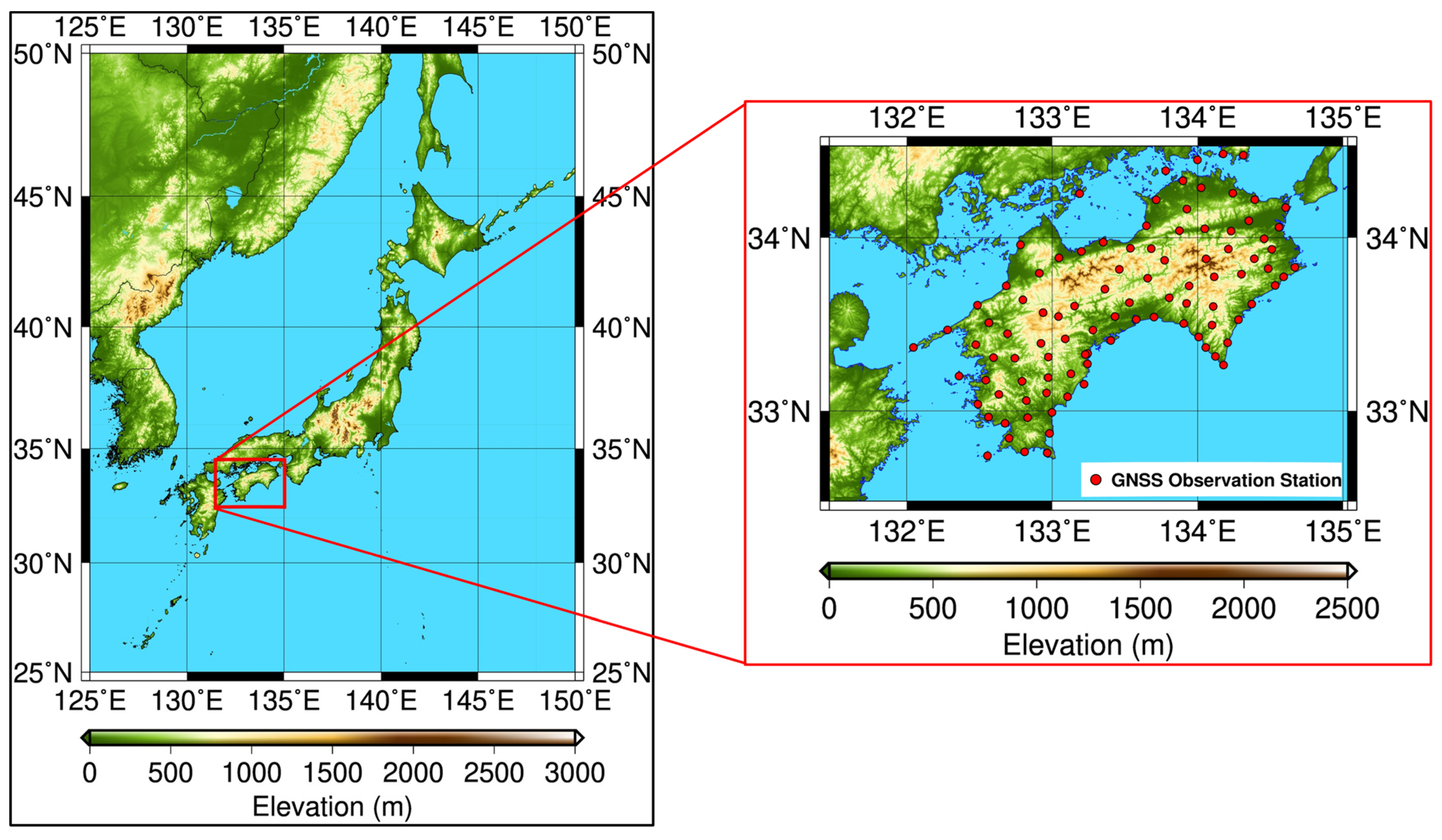
As digital elevation model (DEM) data, the Advanced Spaceborne Thermal Emission and Reflection Radiometer (ASTER) Global Digital Elevation Model (GDEM) data were used. These data were generated using stereo pair images photographed by ASTER sensors mounted on the Terra satellite [30]. The spatial resolution of the ASTER GDEM data was approximately 30 m (1 arc-second). In this study, however, data resampled to a spatial resolution of 90 m were used. Figure 1 depicts the target scope for the study and placement of 98 GNSS observation stations. The base map in Figure 1 shows the ASTER GDEM elevation data converted to a spatial resolution of 90 m.

PW amounts estimated from GNSS data were used to verify the accuracy of PW distributions reproduced using MSM-GPV and ASTER GDEM data. The PW amounts at GNSS observation stations can be estimated from the atmospheric delay of the GNSS signal between the satellite and the ground receiver, as long as the temperature and air pressure at the GNSS observation station are known [31]. The PW amounts estimated from the atmospheric delay of the GNSS signal are referred to as GNSS-PW amounts in this study. Following previous studies [32,33], the GNSS atmospheric delay data at 1-h intervals provided by the Geospatial Information Authority of Japan [34] and the hourly temperature and air pressure values at each GNSS observation station interpolated from the observation values of the Japan Meteorological Agency’s Automated Meteorological Data Acquisition System (AMeDAS) [35] were used to calculate the hourly GNSS-PW amounts in the study.

2.2. Method Used to Reproduce Pecipitable Water Distributions from MSM-GPV and DEM Data

The integrated water vapor amount ($IWV$) can be calculated from radiosonde data using Equation (1) [36].

$$IWV=\frac{100}{g}\left[q_{L1,L0}\left(P_{L0}-P_{L1}\right)+q_{L1,L2}\left(P_{L1}-P_{L2}\right)+\cdots \right],$$

(1)

where $q_{Li,Lj}$denotes the mean value (kg/kg) for specific humidity between the barometric surface $P_{Li}$(hPa) and $P_{Lj}$(hPa), and $g$ represents the standard acceleration of free fall.

Accordingly, the PW distribution with a resolution of 5 km can be calculated with the MSM-GPV data using Equation (2):

$$\begin{gathered} {IWV}_{300}=\frac{100}{g}\left[q_{S,1000}\left(P_s-P_{1000}\right)+q_{\mathrm{1000,975}}\left(P_{1000}-P_{975}\right)+\cdots \\ +q_{\mathrm{400,300}}\left(P_{400}-P_{300}\right)\right] \\ =W_{S,1000}+W_{\mathrm{1000,975}}+\cdots +W_{\mathrm{400,300}}, \end{gathered}$$

(2)

where ${IWV}_{300}$ denotes the cumulative amount of water vapor from the ground surface to the 300-hPa barometric surface level (mm), $P_S$denotes the surface pressure (hPa), $q_S$ denotes the specific humidity at the surface pressure (kg/kg), and $W_{L1,L2}$ denotes the amount of water vapor between the barometric surface $P_{L1}$ and the barometric surface $P_{L2}$ (mm). In this study, ${IWV}_{300}$ was used as the amount of PW.

Next, the specific humidity (kg/kg) at the barometric surface $P_n$ ($q_n$) can be calculated using Equation (3) [36].

$$q_n=\frac{0.622}{\left(P_n/e_{P_n}\right)-0.378},$$

(3)

where $e_{P_n}$denotes water vapor pressure (hPa) at the barometric surface $P_n$.

Moreover, the water vapor pressure (hPa) at the barometric surface $P_n$ ($e_{P_n}$) can be calculated using Equation (4) [36].

$$e_{P_n}=\left(\frac{{RH}_{P_n}}{100}\right)\times e_{P_n,sat},$$

(4)

where ${RH}_{P_n}$ denotes relative humidity (%) at the barometric surface $P_n$, and $e_{P_n,sat}$denotes saturation water vapor pressure (hPa) at the barometric surface $P_n$.

Furthermore, the saturation water vapor pressure (hPa) at the barometric surface $P_n$ ($e_{P_n,sat}$) can be calculated using Equation (5) [36].

$$e_{P_n,sat}=6.1078\times {10}^{\frac{7.5T_{P_n}}{T_{P_n}+237.3}},$$

(5)

where $T_{P_n}$ denotes the temperature ($℃$) at the barometric surface $P_n$.

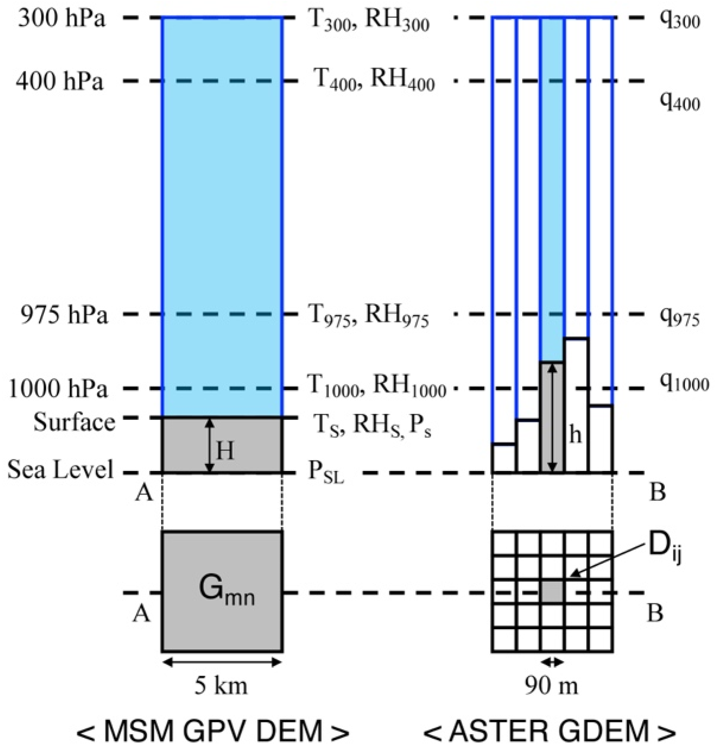
As the MSM-GPV barometric surface data include prediction values for relative humidity and temperature at 12 barometric surfaces between 1000 and 300 hPa, Equations (2)–(5) can be used to calculate the integrated water vapor amount from the ground surface up to the 300-hPa barometric surface level. Moreover, in reproducing PW distributions using the MSM-GPV data and the ASTER GDEM elevation data, PW distributions with a spatial resolution of 90 m can be reproduced by considering the differences in elevation within the 5-km grid squares of the MSM-GPV data using the ASTER GDEM data with a spatial resolution of 90 m (Figure 2). Here the focus is only on the individual grid squares $G_{mn}$ in the MSM-GPV data and the individual pixels $D_{ij}$ in the ASTER data corresponding to the interior of $G_{mn}$. The PW amount at $D_{ij}$ (${PW}_{D_{ij}}$) can be calculated from the specific humidity $q_{D_{ij}}$ and ground air pressure $P_{D_{ij}}$ at $D_{ij}$, which can be estimated using both MSM-GPV and ASTER GDEM data.

Assuming that air is an ideal gas and the temperature lapse rate is 6.5 K/km, the elevation $H_{ G_{mn}}$ of each MSM-GPV data grid square $G_{mn}$ can be calculated using the relational expression shown in Equation (6) [37].

$$H_{G_{mn}}=\frac{T_{G_{mn}}+273.15}{0.0065}\left\{{\left(\frac{P_{SL,G_{mn}}}{P_{G_{mn}}}\right)}^{\raisebox{1ex}{$1$}\!\left/ \!\raisebox{-1ex}{$5.257$}\right.}-1\right\},$$

(6)

where $T_{ G_{mn}}$ denotes the surface temperature ($℃$), $P_{ G_{mn}}$ denotes the surface pressure (hPa), and $P_{SL, G_{mn}}$ denotes the mean sea-level barometric pressure of $G_{mn}$ (hPa).

Next, if the elevation at each DEM pixel $D_{ij}$ is $h_{D_{ij}}$ (m), the surface pressure at $D_{ij}$ ($P_{D_{ij}}$) can be expressed using $T_{ G_{mn}}$, $P_{SL, G_{mn}}$, and $h_{D_{ij}}$ as follows [37]:

$$P_{D_{ij}}=P_{SL,G_{mn}}\times {\left(1-\frac{0.0065h_{D_{ij}}}{T_{SL,G_{mn}}+273.15}\right)}^{5.257},$$

(7)

where $T_{SL, G_{mn}}$ denotes the mean sea-level barometric pressure ($℃$).

The value for $T_{SL, G_{mn}}$ can be derived from Equation (8) as follows:

$$T_{SL,G_{mn}}=T_{G_{mn}}+0.0065H_{G_{mn}}.$$

(8)

In addition, the specific humidity at $D_{ij}$ ($q_{D_{ij}}$) can be calculated using Equation (9) as follows [38]:

$$q_{D_{ij}}=\frac{0.622}{\left(P_{D_{ij}}/e_{D_{ij}}\right)-0.378}.$$

(9)

From Equations (4) and (5), the saturation water vapor pressure at $D_{ij}$ ($e_{D_{ij}}$) can be calculated using Equation (10) as follows:

$$e_{D_{ij}}=\left(\frac{{RH}_{D_{ij}}}{100}\right)\times 6.1094\times exp\left\{17.625T_{D_{ij}}/\left(243.04+T_{D_{ij}}\right)\right\},$$

(10)

where $T_{D_{ij}}$ denotes the temperature ($℃$) at each DEM pixel $D_{ij}$.

The value for $T_{D_{ij}}$ can be determined using Equation (11):

$$T_{D_{ij}}=T_{SL,G_{mn}}-0.0065h_{D_{ij}}.$$

(11)

Finally, if $P_{D_{ij}}$ > 1000 hPa, it can be surmised that ${RH}_{D_{ij}}$ = ${RH}_{G_{mn}}$, and $q_{D_{ij}}$ can be estimated using Equations (8)–(12).

If $P_{D_{ij}}$ > 1000 hPa, the PW amount at $D_{ij}$ (${PW}_{D_{ij}}$) can be estimated using Equation (12).

$$\begin{gathered} {PW}_{D_{ij}}=\frac{100}{g}\left[q_{D_{ij},1000}\left(P_{D_{ij}}-P_{1000}\right)+q_{\mathrm{1000,975}}\left(P_{1000}-P_{975}\right)+\cdots \\ +q_{\mathrm{400,300}}\left(P_{400}-P_{300}\right)\right]. \end{gathered}$$

(12)

If $P_{D_{ij}}$ ≤ 1000 hPa, $q_{D_{ij}}$ can be presumed to be equivalent to the specific humidity $q_{G_{mn}}$ of $G_{mn}$ at the barometric surface $P_n$ that is closest to $D_{ij}$ (in other words, the specific humidity value calculated from the temperature and relative humidity at the barometric surface $P_n$ in the MSM-GPV data). As a result, if $P_{D_{ij}}$ ≤ 1000 hPa, ${PW}_{D_{ij}}$ can be estimated using Equation (13).

$$\begin{gathered} {PW}_{D_{ij}}=\frac{100}{g}\left[q_{D_{ij},1}\left(P_{D_{ij}}-P_{L1}\right)+q_{L1,L2}\left(P_{L1}-P_{L2}\right)+\cdots +q_{\mathrm{400,300}}\left(P_{400}-P_{300}\right)\right], \\ (P_{400}<P_{L2}<P_{L1}<P_{D_{ij}}\le 1000) \end{gathered}$$

(13)

where $P_{L1}$ denotes the barometric surface closest to $P_{D_{ij}}$ in the MSM-GPV data, and$P_{L2}$ denotes the barometric surface closest to $P_{L1}$ in the MSM-GPV data.

In this study, the ${PW}_{D_{ij}}$ value calculated using Equation (12) or (13) is referred to as the MSM-PW.

The amount of water vapor in the atmosphere decreases as the elevation increases [39,40]. Accordingly, if there is a significant discrepancy between the elevation data used for MSM-GPV data calculations and the elevation of the GNSS observation stations, this may result in significant bias [41]. Therefore, to increase the accuracy of PW amounts reproduced from the MSM-GPV data and DEM, the bias caused by the elevation differential must be removed through elevation correction.

Based on previous research, elevation correction has been formalized as shown below [28]:

$${PW}_{{EC}_m,D_{ij}}={PW}_{D_{ij}}-\left(a_m\times h_{D_{ij}}+b_m\right),$$

(14)

where ${PW}_{{EC}_m,D_{ij}}$ denotes the PW amount at $D_{ij}$ after elevation correction, ${PW}_{D_{ij}}$ denotes the PW amount at $D_{ij}$ before elevation correction, and $a_m$and $b_m$ denote monthly elevation correction coefficients.

In this method, the elevation correction coefficients $a_m$and $b_m$are presumed to be constant throughout the month. The elevation correction coefficients are used to calculate the MSM-PW at 3-h intervals for each month using Equations (12) and (13). The monthly mean values for the difference (bias) between the MSM-PW and GNSS-PW amount at pixels that include GNSS observation stations are calculated. Subsequently, the linear regression expression for the monthly mean value for the bias at each GNSS observation station and the elevation of each GNSS observation station is determined, and the inclination and intercept are expressed as $a_m$and $b_m$, respectively.

The PW amounts reproduced through elevation correction using this procedure will be referred to as MSM high-resolution PW amounts.

2.3. Study of Methods for Improving Elevation Correction

In previous research [27], Equation (14) was used to perform an elevation correction for all pixels within the target scope. For some GNSS observation stations in low-elevation regions, however, the RMSE between the GNSS-PW amounts and the MSM high-resolution PW amounts for pixels that included GNSS observation stations became worse after elevation correction. Moreover, at low-elevation GNSS observation stations, the bias of the GNSS-PW and MSM-PW amounts for pixels that included GNSS observation stations did not fit the regression line of the monthly mean difference between the MSM-PW and GNSS-PW amounts at each GNSS observation station and elevation at each GNSS observation station very well. In other words, in high-elevation regions, it was possible to improve the accuracy of reproduced values for PW amount through elevation correction; however, in low-elevation regions, the reproduction accuracy of the PW amount was adversely affected by overcorrection [27]. Accordingly, by conducting elevation correction only for regions, where the elevation exceeds 200 m, it was possible to prevent the RMSE of low-elevation regions from being adversely affected by overcorrection during elevation correction, whereas, in high-elevation regions, it was possible to improve the reproduction accuracy of the PW amount [28]. However, the elevation value that should be used as the standard for conducting elevation correction (200 m in previous studies) could not be determined.

In this study, the fact that the bias of GNSS-PW amounts corresponding to the MSM-PW amounts for pixels that include GNSS observation stations increased at higher elevations was thought to be because of the significant impact of the presumption when the PW amount was calculated using Equation (12). In high-elevation regions, $P_{D_{ij}}$ ≤ 1000 hPa, and when the PW amount is calculated using Equation (12), the specific humidity $q_{D_{ij}}$ at each ASTER GDEM pixel $D_{ij}$ “is assumed equal to the specific humidity value calculated from the temperature and relative humidity at the barometric surface $P_n$ in the MSM-GPV data that is closest to $D_{ij}$”. In other words, as in this case, differences in elevation within the 5-km grid squares of the MSM-GPV data are not considered, and this is thought to be a factor that affects reproduction accuracy in high-elevation regions. Accordingly, in this study, based on Figure 2 and Equation (2), it is thought that in many cases $W_{S,1000}=0$ when $P_{D_{ij}}$ ≤ 1000 hPa, a study was conducted to determine whether $W_{S,1000}$ is equal to or not equal to zero as the threshold value for performing elevation correction.

2.4. Study of Methods for Converting Temporal Resolutions to High-Resolution Values

As the temporal resolution of MSM-GPV data for each barometric surface is 3 h, with the method described in Section 2.1, MSM high-resolution PW amounts can only be reproduced at 3-h intervals. Accordingly, to convert the temporal resolution of MSM high-resolution PW amounts to high-resolution values, the MSM-GPV data for each barometric surface at 3-h intervals should be interpolated to data at 1-h intervals.

Many studies are currently underway to find methods for filling in the regular time gaps in meteorological data [42,43,44]. “Regular gaps” refer to the 2-h-long gaps in 3-h data [42]. Previous studies have attempted to use linear interpolation, Lagrange interpolation, spline interpolation, and so on as methods to fill in these time gaps. The results vary depending on the study in terms of the methods that show a high degree of accuracy; however, in many cases, spline interpolation has exhibited more accurate results than linear or Lagrange interpolation [42,43]. Anjomshoaa and Salmanzadeh reviewed previous studies and concluded that linear interpolation and cubic spline interpolation are the most commonly used methods for interpolating meteorological data, and in many cases, they are the most accurate [42]. Moreover, Liu et al. demonstrated that, although the ideal interpolation method differs depending on the season and the meteorological elements, cubic spline interpolation and the Akima spline interpolation method are highly accurate in most cases [44].

Cubic spline interpolation focuses on the monotonicity and unevenness of each interval function and divides the interpolation interval into multiple partial segments for interpolation. This results in the best approximation and ideal convergence, producing a smooth interpolation curve and providing good interpolation results for meteorological data [44]. The Akima spline interpolation method approximates each partial segment using a cubic polynomial function. Only a portion of the adjacent data is used, the continuity of the first derivation is ensured, and the smoothness, shape retention, and robustness of the interpolation curve are better than those of cubic spline interpolation [44].

Accordingly, in this study, the cubic spline interpolation method and the Akima spline interpolation method were used to construct barometric surface data at 1-h intervals from the MSM-GPV data for each barometric surface at 3-h intervals, and these data were used to calculate MSM high-resolution PW amounts. The method with the best reproduction accuracy would be ultimately used subsequently.

2.5. Reproducibility in Near Real Time

With the method described in Section 2.2, the monthly elevation correction coefficients are obtained after the MSM-PW amounts at 3-h intervals are calculated using the monthly MSM-GPV data. As a result, with existing methods, it was difficult to reproduce the PW distribution in near real time after MSM-GPV data at 3-h intervals had been obtained. In this study, we calculated the elevation correction coefficients for each month using existing methods and reproduced the MSM high-resolution PW from 2019 to 2022. Subsequently, the monthly mean value for the RMSE between the MSM high-resolution PW and GNSS-PW amounts at each GNSS observation station is calculated for each year. The results are compared with the results of the reproduction of MSM high-resolution PW from 2019 to 2022 using the averages of the monthly correction coefficients from 2014 to 2018. If the difference between the monthly average of RMSE using the elevation correction coefficients for each period and the monthly average of the elevation correction coefficients from 2014 to 2018 is small, it is thought that using the mean value for the monthly correction coefficient for the past several years enables the PW distribution to be reproduced in near real time after the acquisition of numerical prediction data.

3. Results and Discussion

3.1. Study of Methods for Improving Elevation Correction

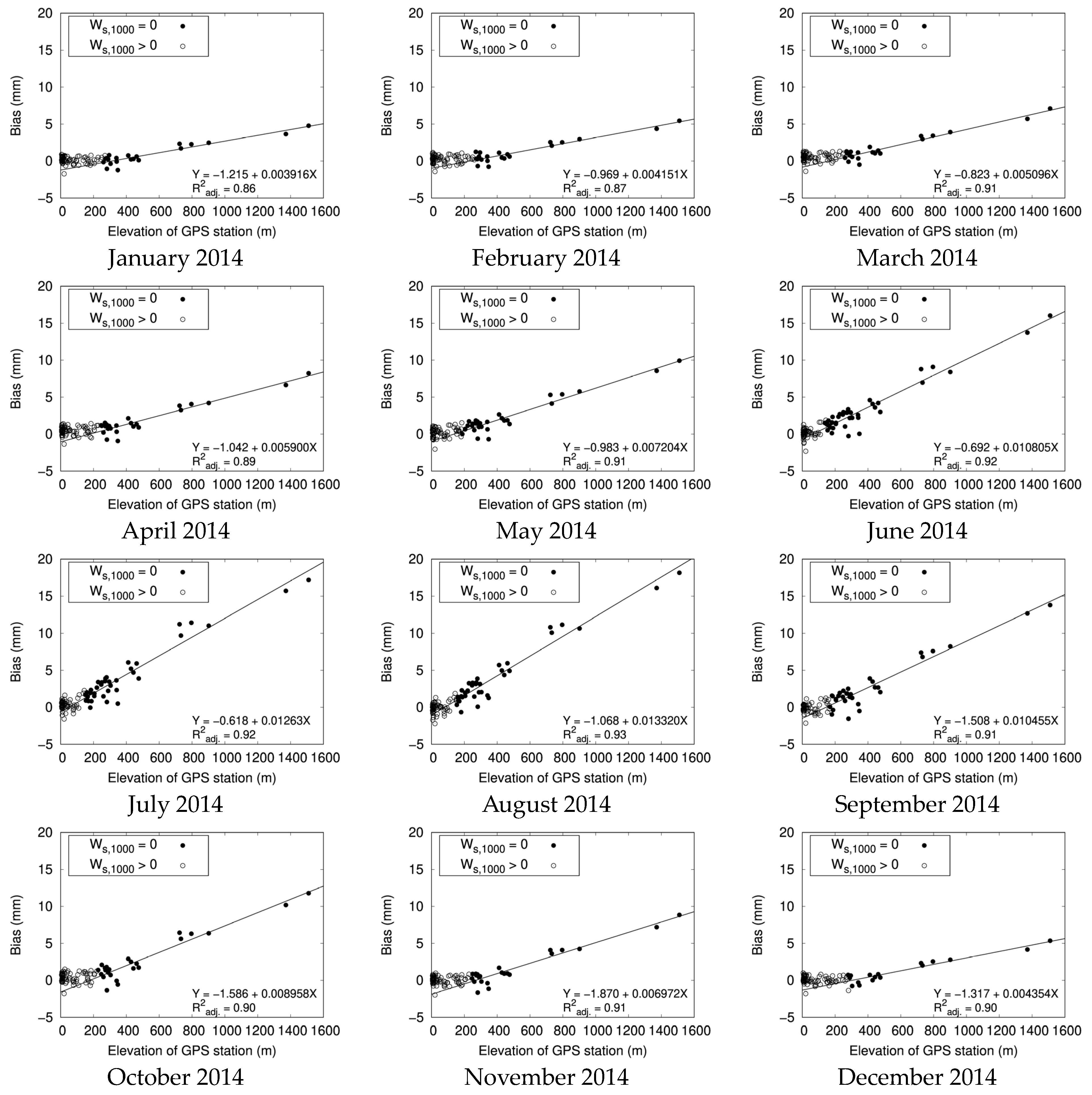
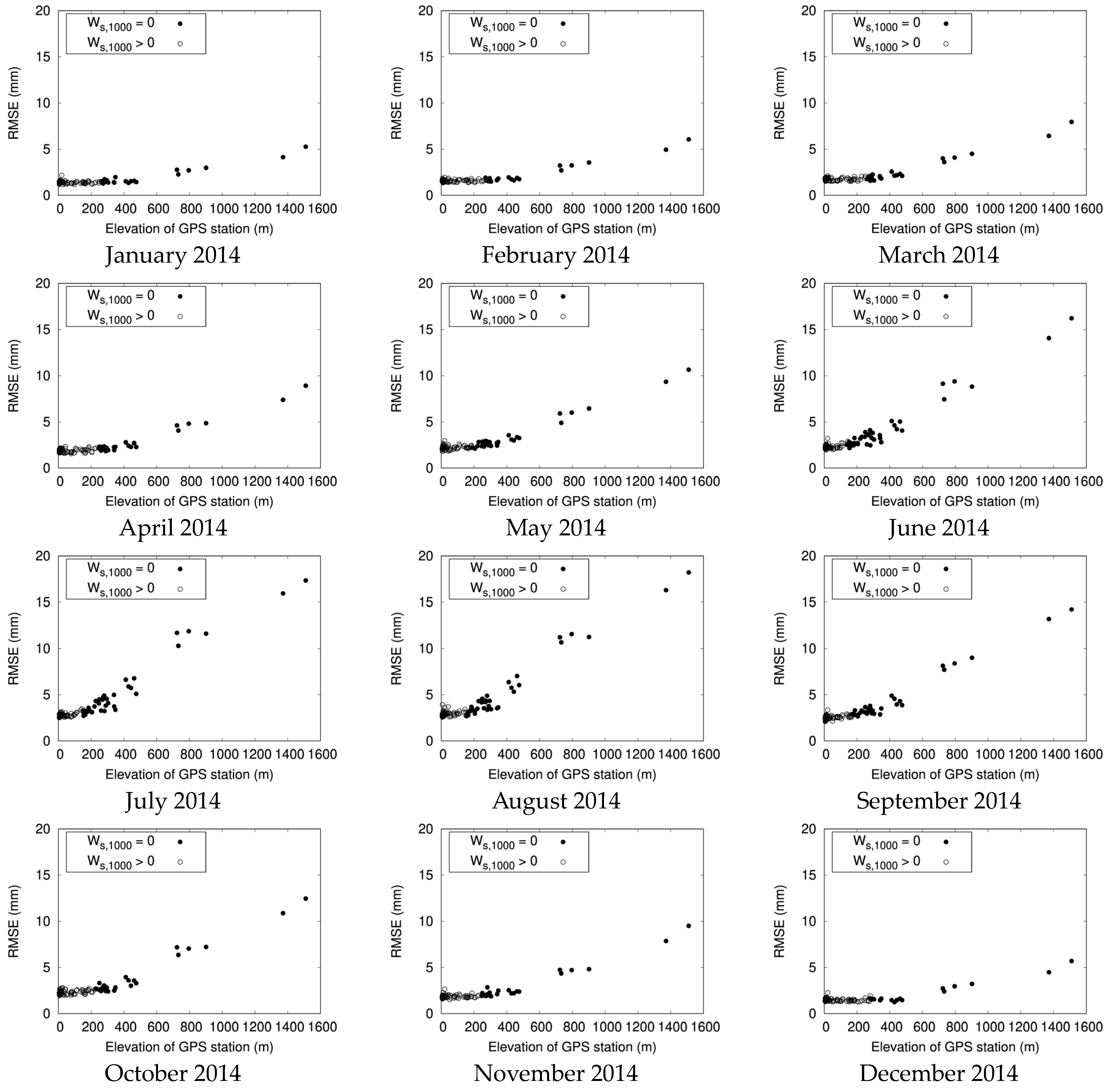
First, MSM-GPV and ASTER GDEM data were used to calculate MSM-PW amounts with a spatial resolution of 90 m. Figure 3 depicts the relationship between the monthly mean value for the bias between the MSM-PW and GNSS-PW amount at each GNSS observation station in 2014 prior to elevation correction and the elevation at each GNSS observation station. Figure 4 depicts the relationship between the monthly mean RMSE for the MSM-PW and GNSS-PW amounts at each GNSS observation station in 2014 and the elevation at each GNSS observation station. In this study, the bias and RMSE were calculated using the GNSS-PW amount treated as the true value. As shown in Figure 3 and Figure 4, the monthly mean values for bias and RMSE at each GNSS observation station are greater for GNSS observation stations at higher elevations. This suggests that the difference between MSM-PW and GNSS-PW amounts prior to elevation correction is highly dependent on elevation. This trend was the same from 2015 to 2022.

Moreover, in Figure 3 and Figure 4, the point configuration differs depending on whether the value for $W_{S,1000}$ is equal to zero. Figure 3 and Figure 4 show that, for GNSS observation stations where $W_{S,1000}$ is equal to 0, the difference between MSM-PW and GNSS-PW amounts is strongly dependent on elevation, whereas, for GNSS observation stations where $W_{S,1000}$ is not equal to 0, the difference between MSM-PW and GNSS-PW amounts is not dependent on elevation. This suggests that regardless of whether $W_{S,1000}$ is equal to or not equal to 0, it can be used as the standard for performing elevation correction.

Next, the MSM-PW at 3-h intervals was calculated for each month using Equations (12) and (13), and at GNSS observation stations where $W_{S,1000}$ is equal to 0, the monthly mean bias with the GNSS-PW amount was calculated. Subsequently, a linear regression expression (Figure 3) was determined for the monthly mean bias of the GNSS observation stations where $W_{S,1000}$ is equal to zero and the elevation at each GNSS observation station, and the inclination and intercept were expressed as monthly elevation correction coefficients $a_m$ and $b_m$, respectively (

Table 3. Monthly elevation correction coefficient $a_m$ (mm/m) and $b_m$ (mm) from 2014 to 2022. The elevation correction coefficient $a_m$ and $b_m$ indicate the slope and intercept of the regression expression for the monthly bias at each GNSS observation station and the elevation of the GNSS observation station, respectively. All values for elevation correction coefficient $a_m$ are statistically significant with a significance level of 5%.

Month	Coefficient	2014	2015	2016	2017	2018	2019	2020	2021	2022
January	$a_m$	3.92 × 10−3	4.26 × 10−3	4.57 × 10−3	4.12 × 10−3	4.11 × 10−3	4.16 × 10−3	5.06 × 10−3	4.04 × 10−3	3.14 × 10−3
	$b_m$	−1.22	−1.23	−1.76	−1.39	−1.64	−1.73	−1.84	−1.15	−0.62
February	$a_m$	4.15 × 10−3	4.26 × 10−3	4.37 × 10−3	4.19 × 10−3	3.53 × 10−3	4.79 × 10−3	4.53 × 10−3	4.24 × 10−3	3.17 × 10−3
	$b_m$	−0.97	−1.05	−1.57	−1.20	−1.45	−1.65	−1.67	−1.14	−0.54
March	$a_m$	5.10 × 10−3	5.32 × 10−3	5.22 × 10−3	4.41 × 10−3	5.27 × 10−3	5.03 × 10−3	5.02 × 10−3	5.70 × 10−3	5.08 × 10−3
	$b_m$	−0.82	−1.63	−1.37	−1.17	−1.52	−1.23	−1.23	−0.99	−0.65
April	$a_m$	5.90 × 10−3	7.69 × 10−3	7.11 × 10−3	6.84 × 10−3	6.63 × 10−3	6.30 × 10−3	4.92 × 10−3	6.06 × 10−3	6.81 × 10−3
	$b_m$	−1.04	−1.98	−1.44	−1.39	−1.15	−0.91	−0.41	−1.02	−1.31
May	$a_m$	7.20 × 10−3	8.17 × 10−3	8.62 × 10−3	8.14 × 10−3	8.13 × 10−3	7.08 × 10−3	8.60 × 10−3	8.72 × 10−3	7.48 × 10−3
	$b_m$	−0.98	−1.79	−1.42	−1.58	−0.63	−0.91	−0.43	−0.90	−0.48
June	$a_m$	1.08 × 10−2	1.07 × 10−2	1.12 × 10−2	9.84 × 10−3	1.06 × 10−2	1.04 × 10−2	1.04 × 10−2	1.04 × 10−2	1.04 × 10−2
	$b_m$	−0.69	−1.51	−0.94	−1.20	−0.62	0.06	0.97	0.00	0.77
July	$a_m$	1.26 × 10−2	1.30 × 10−2	1.34 × 10−2	1.36 × 10−2	1.33 × 10−2	1.22 × 10−2	1.28 × 10−2	1.25 × 10−2	1.27 × 10−2
	$b_m$	−0.62	−1.59	−1.37	−1.01	0.02	0.26	−0.13	0.42	1.20
August	$a_m$	1.33 × 10−2	1.32 × 10−2	1.21 × 10−2	1.30 × 10−2	1.22 × 10−2	1.24 × 10−2	1.32 × 10−2	1.28 × 10−2	1.32 × 10−2
	$b_m$	−1.07	−1.75	0.14	−0.19	0.12	0.50	0.06	0.75	0.96
September	$a_m$	1.05 × 10−2	1.13 × 10−2	1.29 × 10−2	1.09 × 10−2	1.20 × 10−2	1.29 × 10−2	1.14 × 10−2	1.20 × 10−2	1.20 × 10−2
	$b_m$	−1.51	−2.13	−1.45	−1.57	−1.14	−0.58	−0.11	−0.42	−0.04
October	$a_m$	8.96 × 10−3	7.50 × 10−3	1.01 × 10−2	1.01 × 10−2	8.57 × 10−3	9.89 × 10−3	8.52 × 10−3	8.80 × 10−3	8.47 × 10−3
	$b_m$	−1.59	−2.16	−2.45	−2.78	−1.55	−1.31	−1.49	−1.04	−1.23
November	$a_m$	6.97 × 10−3	8.56 × 10−3	7.14 × 10−3	6.40 × 10−3	6.41 × 10−3	6.74 × 10−3	6.94 × 10−3	6.16 × 10−3	6.85 × 10−3
	$b_m$	−1.87	−2.54	−1.99	−2.18	−2.16	−2.35	−1.97	−0.99	−1.04
December	$a_m$	4.35 × 10−3	5.74 × 10−3	5.40 × 10−3	4.03 × 10−3	5.48 × 10−3	5.31 × 10−3	4.52 × 10−3	4.41 × 10−3	4.03 × 10−3
	$b_m$	−1.32	−1.94	−1.85	−1.65	−2.01	−1.88	−1.37	−0.87	−0.95

). All $a_m$ elevation correction coefficients were statistically significant with a significance level of 5%. Moreover,

Table 4. Adjusted coefficient of determination for regression expression for monthly bias at each GNSS observation station from 2014 to 2022 and elevation of GNSS observation station.

Month	2014	2015	2016	2017	2018	2019	2020	2021	2022
January	0.86	0.87	0.89	0.88	0.86	0.90	0.91	0.92	0.83
February	0.87	0.88	0.92	0.91	0.86	0.92	0.91	0.92	0.80
March	0.91	0.89	0.92	0.87	0.89	0.93	0.81	0.93	0.87
April	0.89	0.92	0.89	0.90	0.89	0.89	0.93	0.96	0.90
May	0.91	0.89	0.90	0.88	0.91	0.88	0.95	0.93	0.85
June	0.92	0.90	0.91	0.88	0.89	0.90	0.93	0.91	0.92
July	0.92	0.94	0.90	0.88	0.91	0.88	0.95	0.93	0.89
August	0.93	0.92	0.87	0.88	0.87	0.88	0.94	0.94	0.92
September	0.91	0.91	0.92	0.90	0.92	0.91	0.94	0.94	0.92
October	0.90	0.9	0.90	0.93	0.92	0.92	0.94	0.95	0.92
November	0.91	0.92	0.92	0.90	0.90	0.90	0.93	0.96	0.90
December	0.90	0.90	0.88	0.87	0.94	0.88	0.92	0.93	0.87

shows the adjusted coefficient of determination for the linear regression expression for the monthly mean bias of each GNSS observation station from 2014 to 2022 and the elevation of each GNSS observation station. Although the target regions for analysis differed, the value of the adjusted coefficient of determination for the regression expression increased compared with elevation correction with a 200-m elevation as the threshold, and the fit of the regression expression in this study was improved [28]. When elevation correction was performed using an elevation of 200 m as the threshold, the coefficient of determination decreased to 0.5 or lower in winter when the PW amount was low. However, when elevation correction was performed using $W_{S,1000}$ as the threshold, the coefficient of determination did not decrease even in winter and was constant throughout the year at 0.8 or higher.

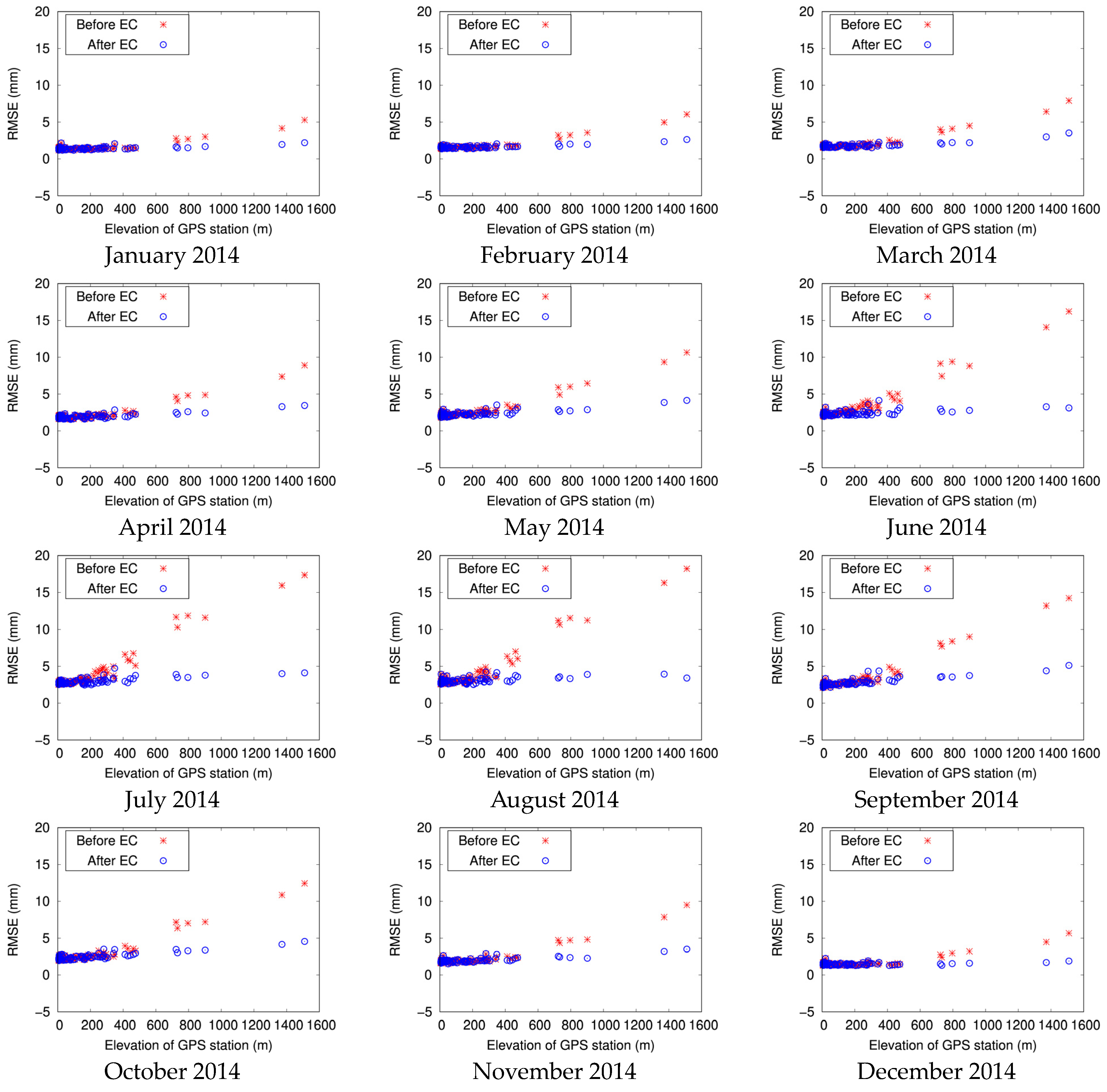
Elevation correction was performed for GNSS observation stations where the value for $W_{S,1000}$ was zero with Equation (14) using the monthly elevation correction coefficients $a_m$ and $b_m$ shown in Table 3. Figure 5 shows the relationship between elevation and the monthly difference (bias) of the MSM-PW and GNSS-PW amounts at each GNSS observation station in 2014. Figure 3 shows that even in the target region of this study, it is possible to visually determine that when the elevation of the GPS observation point is greater than 200 m, the bias value also increases, so it is possible to set the elevation-based threshold value at 200 m in May to October 2014. On the other hand, Figure 3 shows that the value of bias appears to be almost constant until the elevation of the GPS observation point is approximately 400 m, so it is appropriate to set the threshold based on elevation at 400 m in January to April and December 2014. Thus, it can be seen that determining the threshold based on elevation is difficult and can be arbitrary. This study used whether $W_{S,1000}$ is equal to or not equal to zero as the threshold value for performing elevation correction. Figure 5 shows that the elevation dependence of bias between MSM-PW and GNSS-PW amounts with respect to the monthly mean absolute value almost completely disappeared, even for GNSS observation stations where the value of $W_{S,1000}$ became zero because of elevation correction. This trend was the same from 2015 to 2022. This shows that the water vapor amount $W_{S,1000}$ included between the ground and the 1000-hPa isobaric surface can be used in place of elevation as a threshold value for the appropriate application range for elevation correction.

3.2. Study of Methods Converting Temporal Resolution Values to High Resolutions

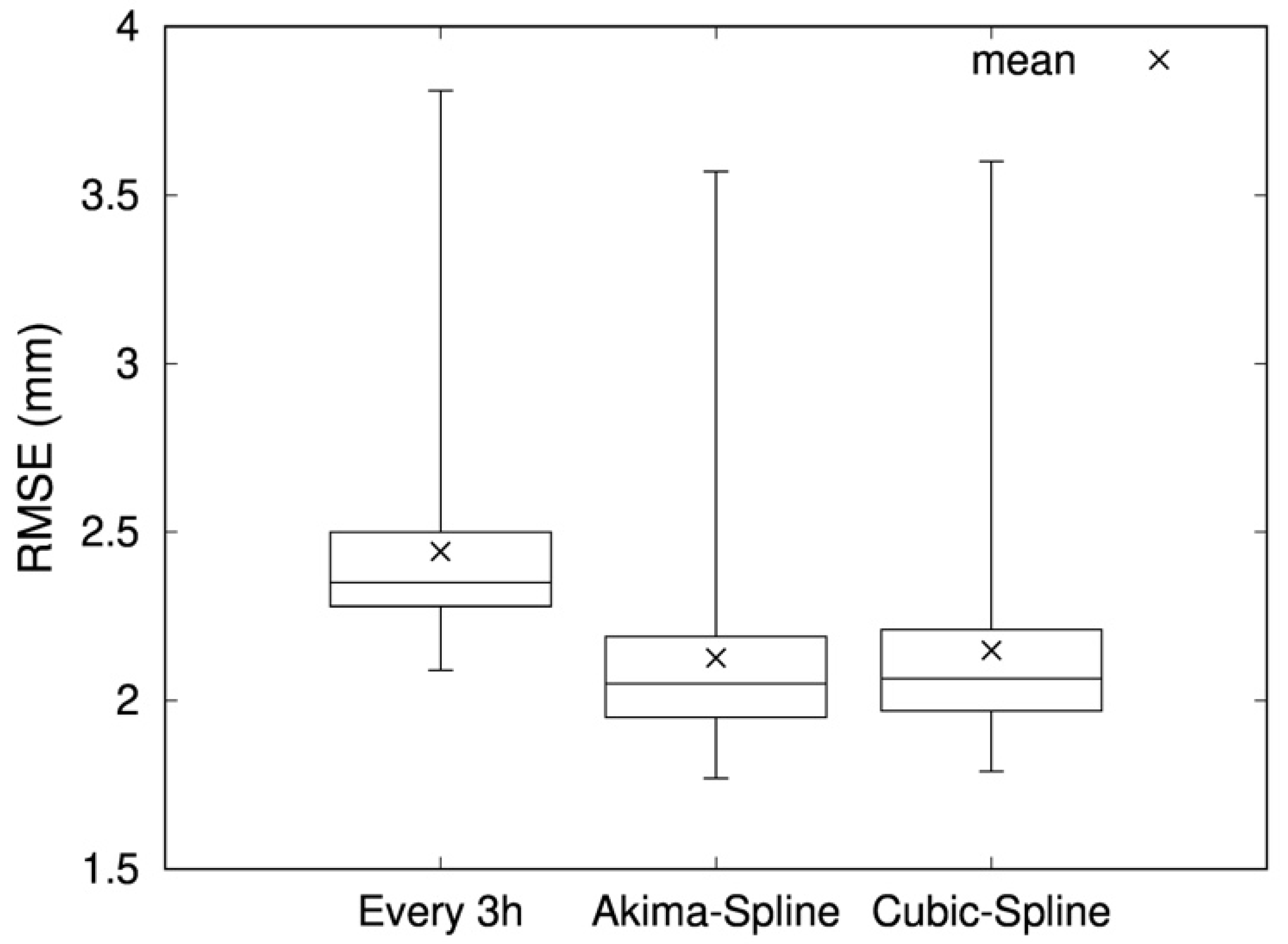
To convert the temporal resolutions of MSM high-resolution PW amounts to high-resolution values, the cubic spline interpolation method and the Akima spline interpolation method were used to construct barometric surface data at 1-h intervals from the MSM-GPV data for each barometric surface at 3-h intervals. Subsequently, the barometric surface data at 1-h intervals were used to reproduce individual MSM high-resolution PW distributions, and the GNSS-PW amounts were used to assess the reproduction accuracy (Figure 6). Figure 6 depicts the RMSE for the MSM high-resolution PW amount at 3-h intervals (midnight, 3 a.m., 6 a.m., 9 a.m., noon, 3 p.m., 6 p.m., and 9 p.m.) at each GNSS observation station, and the RMSE for the MSM high-resolution PW amount at 1-h intervals (1 a.m., 2 a.m., 4 a.m., 5 a.m., 7 a.m., 8 a.m., 10 a.m., 11 a.m., 1 p.m., 2 p.m., 4 p.m., 5 p.m., 7 p.m., 8 p.m., 10 p.m., and 11 p.m.), estimated using the barometric surface data and ground surface data created using the two spline interpolation methods. With regard to the accuracy of the MSM high-resolution PW amount at 3-h intervals reproduced using the ground surface data and barometric surface data at 3-h intervals from the MSM-GPV data, the RMSE 75 percentile values reveal that the RMSE is approximately 2.5 mm or less. Furthermore, even for stations with the worst reproduction accuracy (RMSE is 2.5 mm or less for 75% of all GNSS observation stations in the Shikoku region), the RMSE was 3.8 mm. In contrast, with the MSM high-resolution PW amount at 1-h intervals reproduced using the MSM-GPV ground surface data at 1-h intervals and the barometric surface data at 1-h intervals created using the two spline interpolation methods with MSM-GPV barometric surface data at 3-h intervals, the RMSE 75 percentile values were approximately 2.3 mm or less, suggesting that for 75% of all GNSS observation stations in the Shikoku region, reproduction was possible with an RMSE for each station of 2.3 mm or less. Moreover, even for stations with the worst reproduction accuracy, the RMSE value was 3.6 mm or less. This suggests that, even when barometric surface data created using the two spline interpolation methods are used, PW amounts can be reproduced with equivalent or better accuracy than when using only barometric surface data directly calculated through numerical predictions. In addition, the mean RMSE value for all GNSS observation stations in the Shikoku region was 2.13 mm for the Akima spline interpolation method and 2.15 mm for the cubic spline interpolation method. Accordingly, in this study, the Akima spline interpolation method, which had slightly higher accuracy, was adopted, and an MSM high-resolution PW distribution at 1-h intervals was reproduced by creating barometric surface data at 1-h intervals from the MSM-GPV barometric surface data at 3-h intervals.

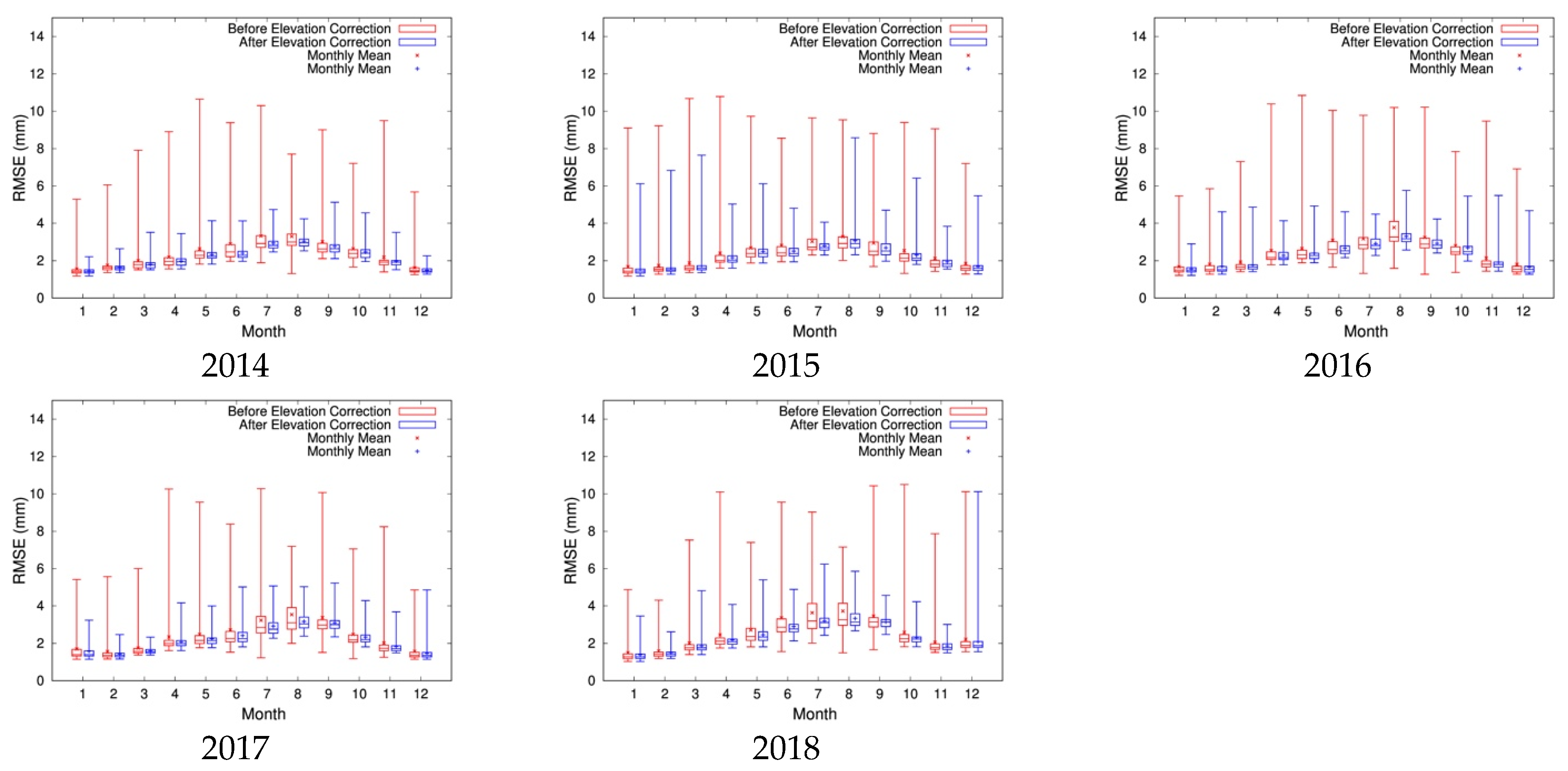
Figure 7 shows the reproduction accuracy of MSM high-resolution PW amounts at 1-h intervals, reproduced using barometric surface data at 1-h intervals generated from MSM-GPV barometric surface data at 3-h intervals using the Akima spline interpolation method. Figure 7 uses box plots to illustrate the monthly mean RMSE at each GNSS observation station from 2014 to 2018. The red box plots show the RMSE values before the elevation correction. The blue box plots show the RMSE values after elevation correction, conducted using $W_{S,1000}=0$ for the water vapor amount$\left(W_{S,1000}\right)$, included between the ground and the 1000-hPa barometric surface, as the threshold for the application range of elevation correction. From the RMSE values in this figure for 75% of the GNSS observation stations in the Shikoku region (in other words, the RMSE 75 percentile values), it was possible to reproduce the PW amount at 1-h intervals from 2014 to 2018 with an RMSE value of approximately 3 mm or lower throughout the year.

3.3. Possibility of Reproduction in Near Real Time

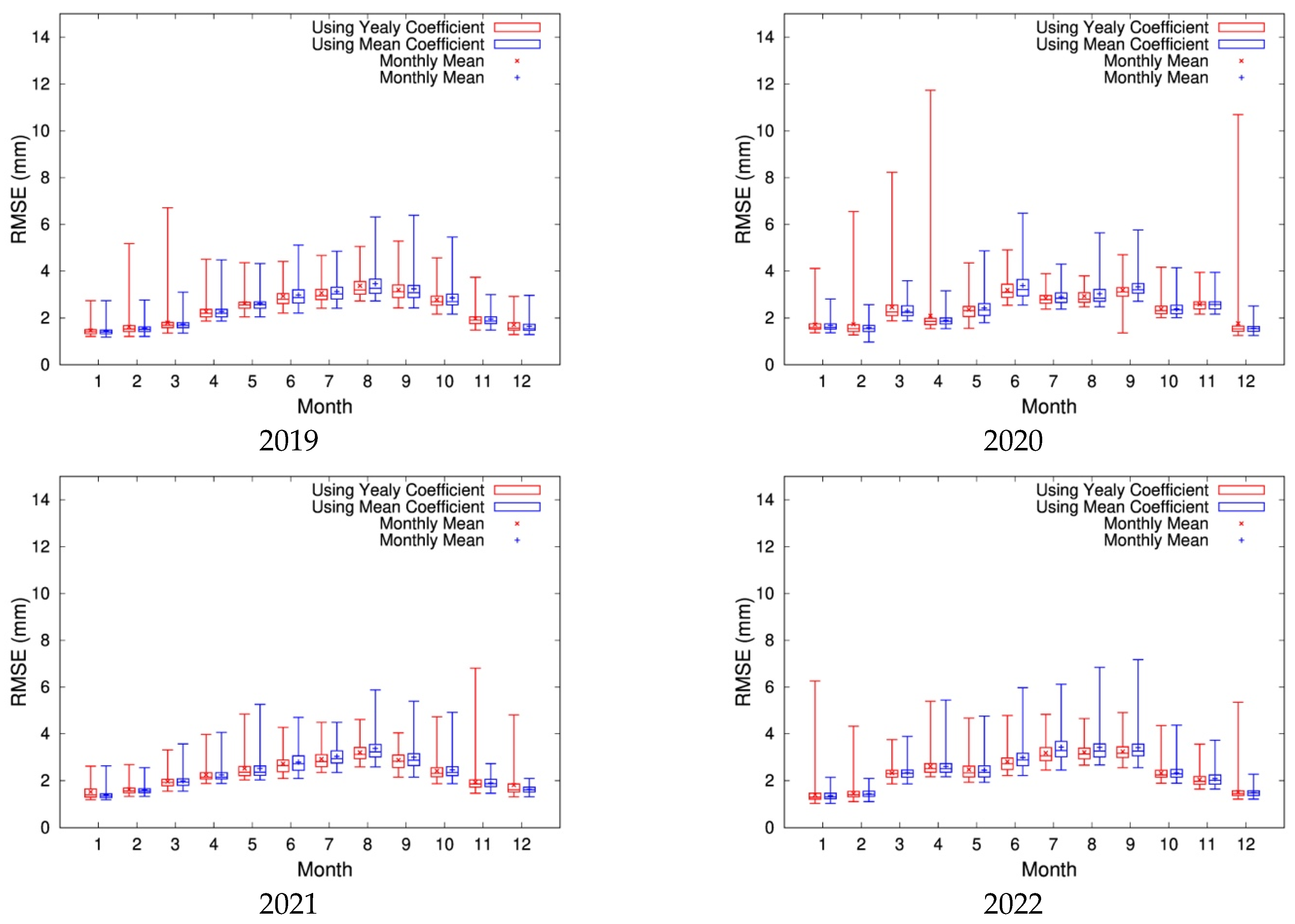
Figure 8 depicts the monthly mean RMSE at each GNSS observation station from 2019 to 2022, shown as box plots. First, the monthly elevation correction coefficients $a_m$ and $b_m$ were determined for each year from 2019 to 2022 (Table 2 and Table 3), and elevation correction was conducted. Then, the MSM high-resolution PW was reproduced, and the mean value for the RMSE of the MSM high-resolution PW and the GNSS-PW amounts at each GNSS observation station was calculated; these values are shown as red box plots. Next, the values $a_m$ and $b_m$ (

Table 5. Mean values for monthly elevation correction coefficients from 2014 to 2018.

Month	Mean
	Slope $\left({\mathit{a}}_{\mathit{m}}\right)$	Intercept $({\mathit{b}}_{\mathit{m}})$
January	4.19 × 10−3	−1.45
February	4.01 × 10−3	−1.25
March	5.05 × 10−3	−1.30
April	6.84 × 10−3	−1.40
May	8.05 × 10−3	−1.28
June	1.06 × 10−2	−0.99
July	1.32 × 10−2	−0.91
August	1.28 × 10−2	−0.55
September	1.15 × 10−2	−1.56
October	9.04 × 10−3	−2.10
November	7.10 × 10−3	−2.15
December	5.00 × 10−3	−1.76

), which are the mean values for monthly elevation correction coefficients for each year from 2014 to 2018, were used as elevation correction coefficients to perform elevation correction for each year from 2019 to 2022 to reproduce the MSM high-resolution PW. Subsequently, the RMSE values for the MSM high-resolution PW and GNSS-PW amounts at each GNSS observation station were calculated; these values are shown as blue box plots. As shown in Figure 8, when the mean values for 2014–2018 are used as elevation correction coefficients, the mean RMSE for each GNSS observation station from June to September tended to be slightly worse. However, a comparison of the RMSE 75 percentile values shows that the degree of worsening of the RMSE values at 75% of all GNSS observation stations in the Shikoku region for a year was extremely small, with the difference in the mean RMSE value at most 0.25 mm (July 2022). Accordingly, this suggests that even if the monthly mean elevation correction coefficients for the past few years are used, the reproduction accuracy of the MSM high-resolution PW would barely worsen. These results show that using the mean value for monthly correction coefficients allows for the reproduction of the PW distribution in near real time following the acquisition of numerical prediction data.

4. Conclusions

This study considered (1) the threshold value for the application range of elevation correction, (2) methods for converting temporal resolutions to high-resolution values, and (3) the possibility of reproducing PW distributions in near real time, with the aim of using numerical prediction data with high temporal resolutions and elevation data with high spatial resolutions to reproduce PW distributions with high spatiotemporal resolutions (90 m, 1 h). The results are as follows.

(1) Using the amount of water vapor included between the ground and the 1000-hPa isobaric surface as a threshold value for the application range for elevation correction in place of elevation enabled elevation correction with equivalent or better accuracy than using elevation as the threshold. When the elevation is used as the threshold, it is difficult to determine the reference elevation value. Moreover, with the method used in this study, the coefficient of determination for the regression expression used to derive the elevation correction coefficient increased compared with the use of elevation as the threshold. Accordingly, it is thought to be appropriate to use the amount of water vapor included between the ground and the 1000-hPa isobaric surface as the threshold for the application range of elevation correction.

(2) The cubic spline interpolation method and the Akima spline interpolation method were used to create barometric surface data at 1-h intervals from the MSM-GPV data for each barometric surface at 3-h intervals, and these data were used to reproduce individual MSM high-resolution PW distributions; subsequently, GNSS-PW amounts were used to assess the reproduction accuracy. The results showed that reproduction was possible with equivalent or better accuracy than when using barometric surface data at 3-h intervals, even in the periods where PW amounts were reproduced using the barometric surface data at 1-h intervals interpolated using the Akima spline interpolation method. For 75% of the GNSS observation stations in the Shikoku region, it was possible to reproduce PW amounts at 1-h intervals with an RMSE of 2.5 mm or less throughout the year. This suggests that using the Akima spline interpolation method to create barometric surface data at 1-h intervals from MSM-GPV barometric surface data at 3-h intervals enables the reproduction of MSM high-resolution PW distributions at 1-h intervals.

(3) To investigate the possibility of reproducing PW distributions in near real time, in this study, a comparison of accuracy was performed for the results of (a) calculation of monthly elevation correction coefficients for each year from 2019 to 2022 and reproduction of individual PW distributions and (b) using the mean values for monthly elevation correction coefficients from 2014 to 2018 to reproduce the individual PW distributions from 2019 to 2022. The results showed that using the mean values from 2014 to 2018 as elevation correction coefficients slightly degraded reproduction accuracy. However, the degree of degradation of the reproduction accuracy was minute over a year, with the degradation of the RMSE value at most approximately 0.25 mm. This shows that using the mean values for monthly correction coefficients for the past few years enables the reproduction of PW distributions in near real time following the acquisition of numerical prediction data.

The above results suggest that, with our proposed method, numerical prediction data and elevation data can be used to reproduce PW distributions in near real time at a spatial resolution of 90 m and a temporal resolution of 1 h, with an RMSE value of 3 mm or less throughout the year.

The method proposed in this study is applicable to the entire range of MSM-GPV data. However, caution is required when applying the elevation correction coefficients of this study to areas other than the target region of this study. It should be mentioned that the spatial versatility of the elevation correction coefficients in this study needs to be evaluated by applying them to areas other than those covered by this study. In that case, it would be better if the entire MSM-GPV data could be analyzed at once instead of narrowing down the target region to a certain region, but it is expected that it would take an enormous amount of processing time to reproduce the PW distribution over the entire region at 90 m resolution. Therefore, reducing processing time to reproduce PW distributions is also a future task, and for this purpose, it is necessary to examine the spatial resolution of the PW distribution sufficient to evaluate the spatial variation of atmospheric water vapor amount. In a study by Vogelmann et al. [25], the scale of spatial variability of atmospheric water vapor amount was noted to be several kilometers, which means that reproducing PW distribution with a spatial resolution coarser than 90 m may be sufficient for evaluating spatial variability of atmospheric water vapor amount. Therefore, if the spatial resolution of the PW distribution sufficient to evaluate the spatial variability of atmospheric water vapor amount becomes clear, processing time for reproducing PW distributions can be reduced. This will enable the analysis of a wider area, so it is expected that spatially versatile elevation correction coefficients can be obtained.

References

- Zhao, Q.; Zhang, X.; Wu, K.; Liu, Y.; Li, Z.; Shi, Y. Comprehensive precipitable water vapor retrieval and application platform based on various water vapor detection techniques. Remote Sens. 2022, 14, 2507. [Google Scholar] [CrossRef]
- Chen, B.; Liu, Z. Global water vapor variability and trend from the latest 36 year (1979 to 2014) data of ECMWF and NCEP reanalyses, radiosonde, GPS, and microwave satellite. J. Geophys. Res. Atmos. 2016, 121, 11–442. [Google Scholar] [CrossRef]
- Wagner, T.; Beirle, S.; Grzegorski, M.; Platt, U. Global trends (1996–2003) of total column precipitable water observed by global ozone monitoring experiment (GOME) on ERS-2 and their relation to near-surface temperature. J. Geophys. Res. 2006, 111, D12102. [Google Scholar] [CrossRef] [Green Version]
- Sarkar, S.; Kuttippurath, J.; Patel, V.K. Long-term changes in precipitable water vapour over India derived from satellite and reanalysis data for the past four decades (1980–2020). Environ. Sci. 2023, 3, 749–759. [Google Scholar] [CrossRef]
- Dai, A. Recent climatology, variability, and trends in global surface humidity. J. Clim. 2006, 19, 3589–3606. [Google Scholar] [CrossRef] [Green Version]
- Mieruch, S.; Schröder, M.; Noël, S.; Schulz, J. Comparison of decadal global water vapor changes derived from independent satellite time series. J. Geophys. Res. Atmos. 2014, 119, 12–489. [Google Scholar] [CrossRef]
- Zhang, L.; Wu, L.; Gan, B. Modes and mechanisms of global water vapor variability over the twentieth century. J. Clim. 2013, 26, 5578–5593. [Google Scholar] [CrossRef]
- Held, I.M.; Soden, B.J. Robust responses of the hydrological cycle to global warming. J. Clim. 2006, 19, 5686–5699. [Google Scholar] [CrossRef]
- Santer, B.D.; Wigley, T.M.L.; Gleckler, P.J.; Bonfils, C.; Wehner, M.F.; AchutaRao, K.; Barnett, T.P.; Boyle, J.S.; Brüggemann, W.; Fiorino, M.; et al. Forced and unforced ocean temperature changes in Atlantic and pacific tropical cyclogenesis regions. Proc. Natl. Acad. Sci. USA 2006, 103, 13905–13910. [Google Scholar] [CrossRef]
- Shoji, Y.; Sato, K.; Yabuki, M.; Tsuda, T. Comparison of shipborne GNSS-derived precipitable water vapor with radiosonde in the western north pacific and in the seas adjacent to Japan. Earth Planets Space 2017, 69, 153. [Google Scholar] [CrossRef]
- He, W.; Cheng, Y.; Zou, R.; Wang, P.; Chen, H.; Li, J.; Xia, X. Radiative transfer model simulations for ground-based microwave radiometers in North China. Remote Sens. 2021, 13, 5161. [Google Scholar] [CrossRef]
- Sun, W.; Wang, J.; Li, Y.; Meng, J.; Zhao, Y.; Wu, P. New gridded product for the total columnar atmospheric water vapor over ocean surface constructed from microwave radiometer satellite data. Remote Sens. 2021, 13, 2402. [Google Scholar] [CrossRef]
- Lu, C.; Chen, X.; Liu, G.; Dick, G.; Wickert, J.; Jiang, X.; Zheng, K.; Schuh, H. Real-time tropospheric delays retrieved from multi-GNSS observations and IGS real-time product streams. Remote Sens. 2017, 9, 1317. [Google Scholar] [CrossRef] [Green Version]
- Van Malderen, R.; Pottiaux, E.; Stankunavicius, G.; Beirle, S.; Wagner, T.; Brenot, H.; Bruyninx, C.; Jones, J. Global spatiotemporal variability of integrated water vapor derived from GPS, GOME/Sciamachy and ERA-interim: Annual cycle, frequency distribution and linear trends. Remote Sens. 2022, 14, 1050. [Google Scholar] [CrossRef]
- Wu, Z.; Liu, Y.; Liu, Y.; Wang, J.; He, X.; Xu, W.; Ge, M.; Schuh, H. Validating HY-2A CMR precipitable water vapor using ground-based and shipborne GNSS observations. Atmos. Meas. Tech. 2020, 13, 4963–4972. [Google Scholar] [CrossRef]
- Kaufman, Y.J.; Gao, B.-C. Remote sensing of water vapor in the near IR from EOS/MODIS. IEEE Trans. Geosci. Remote Sens. 1992, 30, 871–884. [Google Scholar] [CrossRef]
- Li, X.; Tan, H.; Li, X.; Dick, G.; Wickert, J.; Schuh, H. Real-time sensing of precipitable water vapor from BeiDou observations: Hong Kong and CMONOC networks. J. Geophys. Res. Atmos. 2018, 123, 7897–7909. [Google Scholar] [CrossRef] [Green Version]
- Nelson, R.R.; Crisp, D.; Ott, L.E.; O’Dell, C.W. High-accuracy measurements of total column water vapor from the orbiting carbon observatory-2. Geophys. Res. Lett. 2016, 43, 12–261. [Google Scholar] [CrossRef] [Green Version]
- Xiong, Z.; Sun, X.; Sang, J.; Wei, X. Modify the accuracy of MODIS PWV in China: A performance comparison using random forest, generalized regression neural network and back-propagation neural network. Remote Sens. 2021, 13, 2215. [Google Scholar] [CrossRef]
- Song, Y.; Han, L.; Huang, X.; Wang, G. Analysis and evaluation of the layered precipitable water vapor data from the FENGYUN-4A/AGRI over the southeastern Tibetan Plateau. Atmosphere 2023, 14, 277. [Google Scholar] [CrossRef]
- Zhao, Q.; Yao, W.; Yao, Y.; Li, X. An improved GNSS tropospheric tomography method with the GPT2w model. GPS Solut. 2020, 24, 60. [Google Scholar] [CrossRef]
- Li, H.; Wang, X.; Choy, S.; Wu, S.; Jiang, C.; Zhang, J.; Qiu, C.; Li, L.; Zhang, K. A new cumulative anomaly-based model for the detection of heavy precipitation using GNSS-derived tropospheric products. IEEE Trans. Geosci. Remote Sens. 2022, 60, 1–18. [Google Scholar] [CrossRef]
- Zhang, W.; Zhang, H.; Liang, H.; Lou, Y.; Cai, Y.; Cao, Y.; Zhou, Y.; Liu, W. On the suitability of ERA5 in hourly GPS precipitable water vapor retrieval over China. J. Geod. 2019, 93, 1897–1909. [Google Scholar] [CrossRef]
- Steinke, S.; Eikenberg, S.; Löhnert, U.; Dick, G.; Klocke, D.; Di Girolamo, P.; Crewell, S. Assessment of small-scale integrated water vapour variability during HOPE. Atmos. Chem. Phys. 2015, 15, 2675–2692. [Google Scholar] [CrossRef] [Green Version]
- Vogelmann, H.; Sussmann, R.; Trickl, T.; Reichert, A. spatiotemporal variability of water vapor investigated using lidar and FTIR vertical soundings above the Zugspitze. Atmos. Chem. Phys. 2015, 15, 3135–3148. [Google Scholar] [CrossRef] [Green Version]
- Fersch, B.; Wagner, A.; Kamm, B.; Shehaj, E.; Schenk, A.; Yuan, P.; Geiger, A.; Moeller, G.; Heck, B.; Hinz, S.; et al. Tropospheric water vapor: A comprehensive high-resolution data collection for the transnational upper rhine graben region. Earth Syst. Sci. Data 2022, 14, 5287–5307. [Google Scholar] [CrossRef]
- Akatsuka, S.; Susaki, J.; Takagi, M. Estimation of precipitable water using numerical prediction data. Eng. J. 2018, 22, 257–268. [Google Scholar] [CrossRef]
- Akatsuka, S. Improved method for estimating precipitable water distribution using numerical prediction data. Internet J. Soc. Manag. Syst. 2020, 12, sms19-5790. [Google Scholar]
- Research Institute for Sustainable Humanosphere, Kyoto University. Data Form Japan Meteorological Agency. 2017. Available online: http://database.rish.kyoto-u.ac.jp/arch/jmadata/ (accessed on 8 May 2023).
- Jet Propulsion Laboratory, NASA. ASTER Global Digital Elevation Map Announcement. 2017. Available online: https://asterweb.jpl.nasa.gov/gdem.asp (accessed on 8 May 2023).
- Means, J.D. GPS precipitable water as a diagnostic of the North American monsoon in California and Nevada. J. Clim. 2013, 26, 1432–1444. [Google Scholar] [CrossRef]
- Shangguan, M.; Heise, S.; Bender, M.; Dick, G.; Ramatschi, M.; Wickert, J. Validation of GPS atmospheric water vapor with WVR data in satellite tracking mode. Ann. Geophys. 2015, 33, 55–61. [Google Scholar] [CrossRef] [Green Version]
- Vey, S.; Dietrich, R.; Rülke, A.; Fritsche, M.; Steigenberger, P.; Rothacher, M. Validation of precipitable water vapor within the NCEP/DOE reanalysis using global GPS observations from one decade. J. Clim. 2010, 23, 1675–1695. [Google Scholar] [CrossRef]
- Geospatial Information Authority of Japan. GNSS Data Provided Service. Available online: https://terras.gsi.go.jp (accessed on 8 May 2023).
- Japan Meteorological Agency Homepage. Historical Meteorological Data. Available online: https://www.data.jma.go.jp/obd/stats/etrn/ (accessed on 8 May 2023).
- Kondo, J. Atmospheric Science Near the Ground Surface; The University of Tokyo Press: Tokyo, Japan, 2000. [Google Scholar]
- Sakai, T.; Koremura, K.; Niimi, K. Height measurement error of barometric altimeter and its correction. Electron. Navig. Res. Inst. Pap. 2005, 114, 1–13. [Google Scholar]
- Ross, R.J.; Elliott, W.P. Tropospheric water vapor climatology and trends over North America: 1973-93. J. Clim. 1996, 9, 3561–3574. [Google Scholar] [CrossRef]
- Jin, S.; Li, Z.; Cho, J. Integrated water vapor field and multiscale variations over China from GPS measurements. J. Appl. Meteorol. Climatol. 2008, 47, 3008–3015. [Google Scholar] [CrossRef]
- Wang, H.; Wei, M.; Li, G.; Zhou, S.; Zeng, Q. Analysis of precipitable water vapor from GPS measurements in Chengdu region: Distribution and evolution characteristics in autumn. Adv. Space Res. 2013, 52, 656–667. [Google Scholar] [CrossRef] [Green Version]
- Bock, O.; Keil, C.; Richard, E.; Flamant, C.; Bouin, M. Validation of precipitable water from ECMWF model analyses with GPS and radiosonde data during the MAP SOP. QJR Meteorol. Soc. 2005, 131, 3013–3036. [Google Scholar] [CrossRef]
- Anjomshoaa, A.; Salmanzadeh, M. Filling missing meteorological data in heating and cooling seasons separately. Int. J. Climatol. 2019, 39, 701–710. [Google Scholar] [CrossRef]
- Claridge, D.E.; Chen, H. Missing data estimation for 1-6 h gaps in energy use and weather data using different statistical methods. Int. J. Energy Res. 2006, 30, 1075–1091. [Google Scholar] [CrossRef]
- Liu, D.; Sun, T.; Han, Y.; Yan, X. The influence of calculation error of hourly marine meteorological parameter on building energy consumption calculation. Front. Archit. Res. 2022, 11, 981–991. [Google Scholar] [CrossRef]
Figure 1.
Locations of the target region, along with GNSS observation stations. The base map shows the elevation, which was mapped using ASTER GDEM data. The red dots indicate the locations of the GNSS observation stations.
Figure 2.
Relationship between difference in elevation within 5-km grid squares between ASTER GDEM data with a spatial resolution of 90 m and MSM-GPV data and variables used to calculate PW amount.
Figure 3.
Relationship between monthly mean difference (bias) between MSM-PW and GNSS-PW amount at each GNSS observation station in 2014 prior to elevation correction and elevation at each GNSS observation station. The configuration of points differs depending on whether Ws,1000 is equal to or not equal to zero. The straight line indicates the linear regression expression for the monthly mean bias of the GNSS observation stations, where the value of Ws,1000 is equal to 0, and the elevation of each GNSS observation station.
Figure 4.
Relationship between monthly mean RMSE for MSM-PW and GNSS-PW amounts at each GNSS observation station in 2014 prior to elevation correction and elevation at each GNSS observation station.
Figure 5.
Relationship between monthly difference (bias) of MSM-PW and GNSS-PW amounts at each GNSS observation station in 2014 before and after elevation correction (EC), and elevation at each GNSS observation station. The blue symbols indicate the relationship before elevation correction. The red symbols indicate the relationship after elevation correction.
Figure 6.
Comparison of accuracy of MSM high-resolution PW at 3-h intervals (midnight, 3 a.m., 6 a.m., 9 a.m., noon, 3 p.m., 6 p.m., and 9 p.m.) and accuracy of MSM high-resolution PW at 1-h intervals (1 a.m., 2 a.m., 4 a.m., 5 a.m., 7 a.m., 8 a.m., 10 a.m., 11 a.m., 1 p.m., 2 p.m., 4 p.m., 5 p.m., 7 p.m., 8 p.m., 10 p.m., and 11 p.m.) estimated with barometric surface data and ground surface data created using two spline interpolation methods. (The “×” symbol indicates the mean value for all GNSS observation stations.).
Figure 7.
Monthly mean RMSE at each GNSS observation station from 2014 to 2018. Red indicates the RMSE before the elevation correction. Blue indicates the RMSE after elevation correction. The “×” and “+” symbols indicate the mean value for all GNSS observation stations.
Figure 8.
Monthly mean RMSE at each GNSS observation station from 2019 to 2022. The red box plots show the calculation results of elevation correction coefficients for each period and the reproduction of PW distributions from 2019 to 2022. The blue box plots show the calculation results of elevation correction coefficients for each period from 2014 to 2018 and the use of these monthly mean values to reproduce the PW distributions from 2019 to 2022. The “×” and “+” symbols indicate the mean value for all GNSS observation stations.