Article

Assessment of CH4 and CO2 Emissions from a Gas Collection System of a Regional Non-Hazardous Waste Landfill, Harmanli, Bulgaria, Using the Interrupted Time Series ARMA Model

1
Ekoresurs Harmanli Ltd., 6450 Harmanli, Bulgaria
2
Department of Applied Ecology and Animal Hygiene, Faculty of Agriculture, Trakia University, 6000 Stara Zagora, Bulgaria
3
Department of Pharmacology, Animal Physiology and Physiological Chemistry, Faculty of Veterinary Medicine, Trakia University, 6000 Stara Zagora, Bulgaria
4
Department of Informatics and Mathematics, Faculty of Economics, Trakia University, 6000 Stara Zagora, Bulgaria
5
Department of Biochemistry, Microbiology and Physics, Faculty of Agriculture, Trakia University, 6000 Stara Zagora, Bulgaria
*
Author to whom correspondence should be addressed.
Atmosphere 2023, 14(7), 1089; https://doi.org/10.3390/atmos14071089
Submission received: 17 May 2023 / Revised: 16 June 2023 / Accepted: 27 June 2023 / Published: 29 June 2023
(This article belongs to the Section Air Quality)

Abstract

:
Municipal solid waste (MSW) landfills are among the major sources of greenhouse gas (GHG) emissions affecting global warming and the Earth’s climate. In Bulgaria, 53 regional non-hazardous waste landfills (RNHWL) are in operation, which necessitates conducting studies to determine the environmental risk from the emitted GHGs. This study attempted to assess the CH4 and CO2 emissions from three gas wells of a cell (in active and closed phases, each of 2.5 years duration) in an RNHWL, Harmanli (41°54′24.29″ N; 25°53′45.17″ E), based on monthly in situ measurements by portable equipment, using the Interrupted Time Series (ITS) ARMA model. The obtained results showed a significant variation of the CH4 and CO2 concentrations (2.06–15.1% v/v) and of the CH4 and CO2 emission rates (172.81–1762.76 kg/y) by gas wells (GWs), months and years, indicating the dynamics of the biodegradation of the deposited waste in the areas of the three GWs. Throughout most of the monitoring period (2018–2022), the CH4 concentrations were higher than the CO2 concentrations (% v/v), while CO2 emissions were lower than CH4 emissions (kg/y), a fact that could be explained by the differences in the mass of the two gases. The emissions rates of both gases from GW2 dominated over those from GW1 and GW3, giving a reason to determine the zone of GW2 as a hotspot of Cell-1. On the whole, CH4 and CO2 emission rates were higher in the winter (December–February) and partly in the spring (March–May) compared to summer–autumn (June–November). However, the CH4 and CO2 concentrations and emissions decreased drastically after the Cell-1 closure. The CH4/CO2 ratio (0.68–2.01) by months and gas wells demonstrated a great sensitivity, making it a suitable indicator for the assessment of organic waste biodegradation level in the landfills. The ITS ARMA model confirmed the negative and significant effect of the cell closure on CH4 and CO2 emissions; the correlations found between predicted and observed values were strong and positive (0.739–0.896).

1. Introduction

The rapid urbanization and population growth around the world has resulted in a drastic increase of municipal solid waste (MSW) generation [1,2,3]. The MSW amount is increasing even faster than the rate of urbanization [4]. In recent years, human activities have generated approximately 2 billion tons of MSW annually with an expected growth up to 3.76 billion tons by 2050 [5], of which between 44 and 46% (by mass) will be organic waste (food, plant residues, paper, wood) [6]. Despite the different options for MSW management—prevention, minimization, reuse, recycling, energy recovery, burning, etc.—MSW landfilling is still the most common method for MSW treatment in many countries [7,8,9,10,11]. Approximately 60–85% of the global MSW is deposited in landfills of different types [2,5,12,13]. A number of studies report that MSW landfills may negatively affect the environment (pollution of air, soil, and groundwater) and human health due to the generation of landfill gas (LFG) and leachate [10,14,15,16,17,18,19,20]. Based on literature data, the emissions from the landfills can be classified into five different sources: biogas emissions; landfill leachate emissions; emissions related to the disposal of fresh waste (“fresh waste emissions”); emissions from the temporarily covered landfill surface; and emissions from the permanently covered landfill surface [21]. The correct choice of site for the construction of the landfill is of key importance. Recent research data provide evidence that multi-criteria analysis and geographic information systems are successfully used to find a suitable landfill site location. The method includes three steps: the first step is to process 15 environmental and socio-economic factors utilizing the fuzzy analytic-hierarchy process method; the second step comprises visual analysis and the selection of the most suitable locations from the synthetic convenience map; the third step involves the final ranking of sites by means of the fuzzy multi-objective analysis by ratio plus the full multiplicative form method, based on four additional beneficial and non-beneficial criteria [22]. That is why the adequate management of landfills through their whole life cycle is important to mitigate the potential environmental and human health impacts of MSW landfilling [8,23,24,25].
MSW landfills are a large source of anthropogenic greenhouse gas (GHGs) emissions with a contribution rate of between 69% and 95% in the waste sector [26] and about 3–5% of the total GHG emissions, mainly due to uncontrolled biogas emissions. All this defines landfills as prominent contributors to global warming [24,27,28]. LFG production in the landfills as specific anthropogenic ecological systems depends on many factors: type of the landfill (sanitary or unsanitary), structural features of the site, type of the landfilling (controlled or uncontrolled), amount of the deposited waste, waste type and composition, landfill daily cover, gas and leachate systems design and operation, environmental factors (temperature, moisture content, pH, inhibitory compounds, type of microorganisms—aerobic/anaerobic and their activity), etc. [11,29,30,31,32]. LFG production involves three stages—anaerobic bacterial decomposition of the organic substances, chemical reactions and volatilization or hydrolysis, acetogenesis, and methanogenesis [33,34,35]. LFG is a mixture of different gases divided into two groups; the first group comprises gases generated in large amounts (principal gases—CH4: 55–60% v/v and CO2: 40–45% v/v), while the second group is formed by gases present in very small amounts (minor and trace gases—N2O, H2S, H2, NH3, and non-methane volatile organic compounds/NMVOCs/, about 1–9% v/v) [3,30,36,37].
Generally, the production of CH4 in landfill MSW dominates compared to that of CO2 [31,32,38,39]. Moreover, the global warming potential of methane is 21–36 times higher than that of CO2 over a 100-year time frame and ~80–84 times higher in the short-term as CH4 is a short-lived greenhouse gas—about 12 years [24,31,40,41,42]. In addition to being a potent GHG, CH4 is also an ozone precursor and thus has impacts on air quality, human health, and plants [43,44,45]. The relatively high percentage of CH4 in LGE indicates active anaerobic decomposition of the biodegradable organic waste components [46], while the lower percentage of CO2 is a result of the decomposition of substrates with a high hydrogen/oxygen ratio (e.g., fats, hemicellulose, etc.) as well as its dissolution in water/leachate within the site [27]. Some researchers propose the CH4/CO2 volumetric ratio as a reliable indicator for the assessment of the degradation level of the organic compounds for determination of the anaerobic “age” of the landfill [8,46,47]. Under normal condition closure, landfill sites continue to generate LFG until the organic compounds in the waste are degraded, which can last decades [29,31,46,48] and even centuries [13]. Landfill sites are estimated as the second largest source of anthropogenic CH4 emissions [49], responsible for between 5.0 and 20% of the global methane emissions [41,50,51]; in Europe, that percentage is about 20% [52]–22% [29].
Over the last two decades, EU waste management policy has increasingly shifted the focus with regard to municipal waste from disposal methods to prevention and recycling, to reduce the pressure on the environment and create jobs [53]. In 2020, the EU-28 have generated 225 million tons of MSW—by 13.6% more compared to 1995 (198 million tons)—but the total MSW landfilled in 2020 fell by 69 million tons, or by 58 % compared to 1995 (from 121 million tons to 52 million tons). As a result, the landfilled MSW of the total generated MSW in the EU countries dropped from 61% in 1995 to 32.2% in 2020. Nevertheless, the MSW landfilling is still the most widely used practice in EU countries [54]. For the same period, the CH4 emissions from the solid waste deposition sector also decreased by 37%—from 127 Mt CO2eq to 80 Mt CO2eq. Thus, EU countries contribute to climate change mitigation and air quality and human health improvement [45]. The positive trend towards CH4 emissions reduction can be attributed to the implementation of Directive 31/1999 on landfill [55], binding Member States to reducing the amount of biodegradable municipal waste going to landfills to 35% in 2016 and to 10% until 2035. The Directive has encouraged EU countries to adopt different strategies to avoid sending the organic municipal waste fraction to landfills through composting (including fermentation), incineration, and pre-treatment, such as mechanical-biological treatments (including physical stabilization) [54].
Following the EU waste management policy, in the last decade, Bulgaria (111,000 km2, population 6,520,000) has constantly reduced the amount of MSW generated (from 3572 thousand tons in 2011 to 2829 thousand tons in 2020) as well as the amount of MSW landfilled (from 72% in 2011 to 29% in 2020) [56]. One of the measures to achieve the main goal of the new National Waste Management Plan 2021–2028 [57], namely reducing the impact of harmful waste on the environment and public health, is to apply environmentally friendly practices of MSW landfilling and LFG emission control. Nowadays, 53 regional sanitary non-hazardous MSW landfills with different structures and capacities are in operation in the country. All landfills are constructed and function using a similar technology with minor modifications according to specific conditions of each site. In general, the construction and management of the landfills complies with the EU Landfill Directive [55]. The sanitary landfill construction includes four specific layers that play an important role in the entire process of waste decomposition; the first layer is at the bottom, made of compact clay and a synthetic geomembrane to protect the underground area of pollution; the second layer is a drainage system to drain away the leachate; the third layer is a gas collection system to extract the LFG and the fourth layer forms the repository in which to store the deposited waste. The biogas well-pipes collection system with LFG flaring and daily, temporary, and final covers with the available native soil of the landfill site, followed by its reclamation as the general LFG management practice. The mentioned practices are widely used to control LFG emissions from the landfills in many countries over the world [20,49,58,59]. According to the requirements of Ordinance No. 6/2013 [60], Bulgarian landfill operators are obliged to carry out monitoring on GHG emissions on their own and to report annually collected data to the National Environmental Executive Agency.
The future actions of the authorized Bulgarian institutions regarding the management of MSW and their landfilling follow the EU policy, which aims to achieve a “circular economy” and “zero waste” up to 2050. In this regard, it is planned to build installations for the separation/pretreatment of waste and installations for composting green and other biodegradable waste at all landfills. Currently, 22 bio-waste recovery plants are in operation, another 30 are in the process of implementation and one is in the process of evaluation; of the separation/pretreatment plants—25 are in operation, 21 are in the process of implementation, two are at the working project stage, one is in the process of evaluation and there is an investment intention for another one. There are also ongoing procedures for closing landfills that do not meet the regulatory requirements, as well as procedures for the reclamation of landfills whose capacity has already been filled. The intention is to carry out the technical reclamation of the landfills in the shortest possible terms to prevent the negative impact on the environment from possible self-ignition of the landfilled waste and from other incidents. The building of additional cells to landfills in regions where significant amounts of MSW are generated has been devised. All this creates more favorable and environmentally friendly conditions for landfilling and landfill management in the country [57].
With regard to a more appropriate national policy on the management of non-hazardous MSW landfills and the implementation of more appropriate measures in compliance with the local conditions in the country, it is necessary to conduct scientific research to provide reliable information about the processes in landfills in both active and closed phases. As pointed out by [48], the first step in controlling and managing LFG is to determine the quantity of CH4 and CO2 emissions as those gases are the basic greenhouse gases emitted from the landfills [34,61]. It is strongly suggested to collect biogas emission samples directly at the extraction wells or at the inlet of the LFG combustion facilities [21]. The aim of this study was to assess the CH4 and CO2 emissions from a gas collection system of a cell in a regional non-hazardous waste landfill—Harmanli, Bulgaria—on the basis of: (1) in situ measured concentrations of both gases during the active and closed phases of the cell; (2) the results from statistical and correlation analysis, using the Interrupted Time Series ARMA Model.

2. Materials and Methods

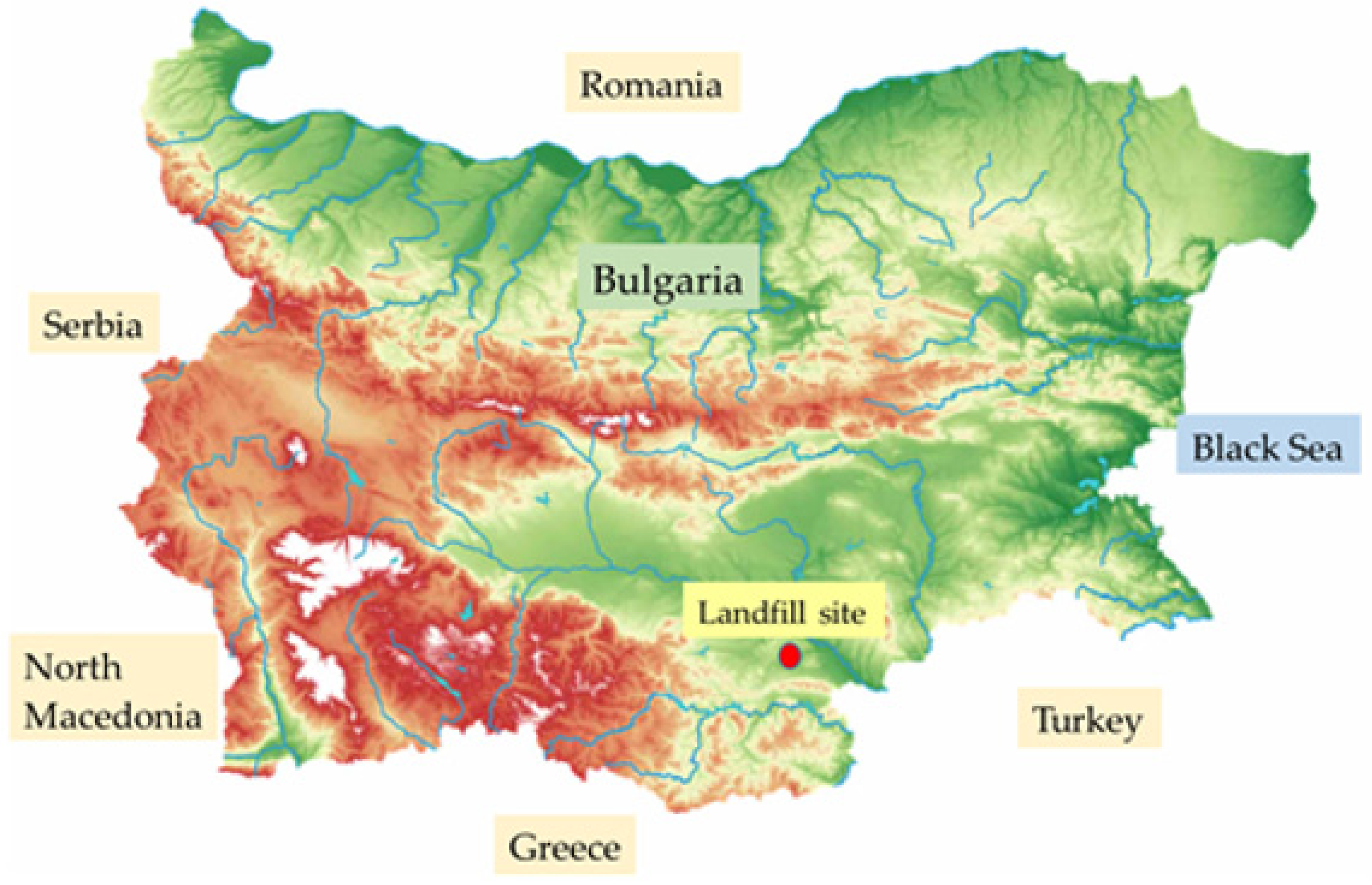
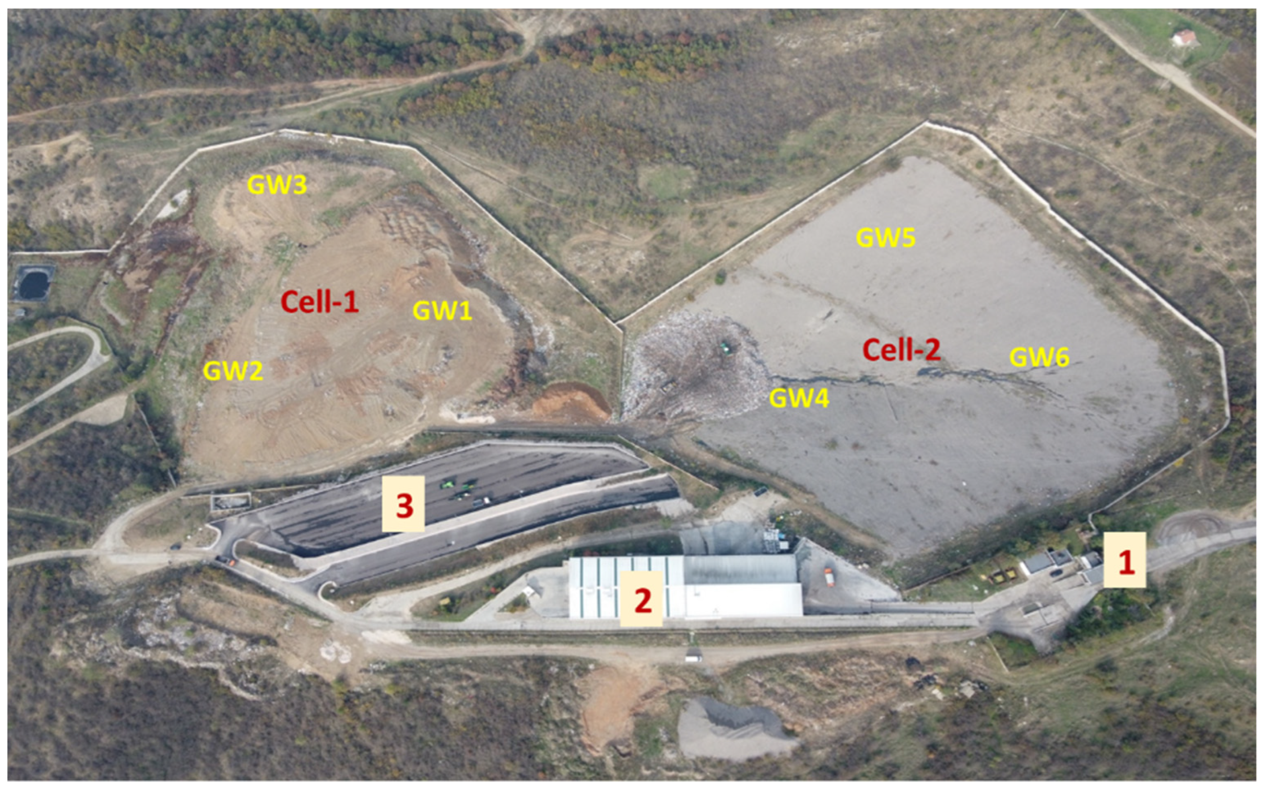
2.1. Site Description

The regional non-hazardous waste landfill (RNHWL) under study is located 2.5 km south of Harmanli town (41°54′24.29″ N; 25°53′45.17″ E; 70 m asl) in Southeast Bulgaria on a surface area of 10.3 ha (Figure 1). The climate of the region is Transitional-Mediterranean—Cfa by the Köppen climate classification. The Mediterranean climatic influence is mainly expressed by the higher average annual temperatures. The micro-climate of the investigated site is characterized by an average annual air temperature of 18.4 °C (maximum average monthly temperature of 28.0 °C—August and minimum of −5.0 °C—January; average annual temperature amplitude 20–22°C), precipitation of 550–600 mm (with autumn–winter rainfall maximum and summer minimum; a secondary precipitation maximum in May), and about 2220 h of sunshine (from 59–69 h in December–January to 320–325 in July–August). The first snow cover forms in the middle of December and in recent years the average annual number of days with snow cover is about five; winter precipitation is mostly rain. Cloud cover is greatest in the winter months, with a score of 6.4 to 6.9, during which the heat flow to the Earth’s surface in the region decreases by about 67%. The average annual total cloud cover is 5.2 points. On average, there are 40.2 days per year with fog; the foggiest days are during November and December. The relative air humidity is within the range 42–77% with a minimum in July and a maximum in January, with an annual average of around 59%. The Harmanli area is characterized by a windy spring with the highest average wind speed in April. The orographic features of the region influence the direction and speed of the wind, with winds with a southern component (SE, S, SW) prevailing. The average annual wind speed is 3.3 m/s [62].
The RNHWL has been in operation since 2003 (Complex Permit No 285-H2/2018) and accepts MSW from seven municipalities with a total of 74,270 inhabitants. The landfill site is a small ravine situated on an east–west slope (23–30°) and consists of two cells for non-hazardous waste: Cell-1, 4.0 ha, capacity 292,254 t and Cell-2, 3.2 ha, capacity 157,102 t, a facility for waste separation, capacity up to 30,000 t/y and a composting facility, capacity up to 2756 t/y (Figure 2). The west borders of the two cells, their lowest parts, are formed with retaining earth dikes: Cell-1—length 41.00 m, height 6.50 m, width in the top 3.00 m and Cell-2—20.00 m, 5.00 m and 3.00 m, respectively. To prevent soil and groundwater pollution, the bottom and the side boundaries of the cells are covered with several layers: a dense and compact clay layer (0.50 m), a geomembrane of high-density polyethylene (HDPE), geotextile, and old car tires covered by sand and gravel (0.50 m, fraction 16–32 mm). Both cells are equipped with a drainage system for leachate treatment and a passive LFG collection and extraction system. The drainage system is constructed by perforated (6.00–22.00 mm) HDPE pipes (Ø 315 mm) and HDPE collector pipe (Ø 355 mm) for taking the leachate to a pumping station. The leachate collected in the pumping station is pumped back over the deposited waste in the cells, mostly during rain.
The LFG collection and extraction system of one cell includes three gas wells (GWs), each of them consisting of a vertical perforated HDPE pipe (Ø 50 mm, 4.00 m), a collector and three perforated horizontal HDPE pipes (Ø 50 mm, 25 m). The vertical pipe is fixed in the center of a cylindrical body of gravel (0.80/1.80 m, fraction 30–50 mm) built by concrete rings with a total height of 1.80 m, the maximal level of the deposited waste in the cell; 0.60 m of the pipe above this level is placed in a metal tube (d = 0.60 m) filled with gravel (fraction 30–50 mm), the rest of the pipe (1.60 m) remaining free. The collector is installed at the bottom of the well and connects the well with the horizontal pipes, placed in the drainage layer in three directions (120° apart) with an upward slope of 1% towards to the collector. The generated LFG is transported to the vertical pipe of the gas well under its own pressure and emitted in the atmosphere.
The daily accepted MSW in the landfill is disposed by layers. The waste is spread by a bulldozer (Shantui SD16, 17 t, Shantui Construction Machinery Co., Ltd., Jining, China) and compacted with a 32 t compactor machine (Hanomag GL 66 D, Hanover, Germany) until a layer with a thickness of 25–40 cm is formed. At the end of the day, the compacted waste layer is covered with native soil and other inert materials about 0.20 m thick. These operations are repeated until the designed thickness (1.80 m) of the landfill waste in the cell is reached. Finally, the temporarily covered cell is closed and prepared for reclamation.
The characteristics and composition of the deposited MSW are listed in Table 1 and Table 2. The data in the two tables were collected from their own monitoring, which the landfill operator is obliged to carry out according to Ordinance No. 6 of 27 August 2013 [60]. Based on the methodology approved by the Ministry of the Environment and Water [63], the settlements in the territory from which the MSW is collected are distributed in two zones: Zone 1, which includes seven cities with a population of 3000 to 25,000 inhabitants and Zone 2, which includes villages with a population of up to 3000 inhabitants. All parameters, included in Table 1—fractional composition, moisture content, bulk weight of the waste, weight of compacted waste (without daily accepted waste and degree of waste compaction) were determined annually, and during the four seasons, two samples were taken for analysis—one sample from Zone 1 and one sample from Zone 2. The formation of an average sample for the analysis of these parameters goes through several stages: Stage 1—the vehicle with waste that arrived at the landfill is weighed on an electronic scale installed at the entrance to the landfill, after which it is directed to a concrete platform for unloading; date and time of arrival, air temperature, and weather conditions are recorded and the waste compaction is visually assessed; Stage 2—after unloading the waste at the site, a visual inspection is performed for the presence of non-domestic waste or hazardous waste; if there are any, they are removed; Stage 3—the obtained waste sample is mixed until a relatively uniform composition is obtained in the different points of the waste pile; Stage 4—the waste is spread in the form of a circle with a height of 30–40 cm; Stage 5—the resulting configuration is divided into four equal parts with solid wooden partitions (i.e., first quartering is carried out); Stage 6—the separated waste in the two diagonally opposite quarters is removed and deposited; the remaining amount of waste is again spread into a circle and a second quartering is carried out; Stage 7—the procedure is repeated until obtaining an average sample of about 120–150 kg. After that, the determination of individual parameters begins as follows: (a) fractional composition—the amount of the received waste sample is successively sifted through sieves with hole sizes of 150 mm and 65 mm, resulting in waste distributed in three fractions (0–65 mm, 65–150 mm and above 150 mm); (b) moisture content, %—BDS EN 15934:2012 (gravimetric) [64]; (c) bulk weight of accepted waste, kg—gravimetric, is determined by the difference in the weight of a container (1 m3) filled with waste from the sample and its weight after emptying; (d) weight of the compacted waste, kg—gravimetric, the procedure is the same as for the determination of bulk weight of the accepted waste, but an average sample of compacted waste (by compacting machine) is used.
When determining the fractional composition of the waste, an average waste sample was also prepared, and this procedure include nine stages. The first seven stages are repeated as for the above-cited parameters. Stage 8—from the average sample of waste determined in Stage 7, the large fractions of the different types of waste are manually removed and are collected in separate plastic bags; the remaining amount of waste is sifted through a sieve with a hole size of 4 mm; sifted waste is classified as inert materials; Stage 9—the bags with the different waste are weighed on an electronic scale ± 0.1 kg, and the results are recorded. Data by types of waste from all of 8 samples during the year are averaged and presented in percentages.
The study was carried out on Cell-1 of the RNHWL for a 5-year period, 2018–2022, and comprised two phases: Phase 1—active cell (from January 2018 to June 2020, when the cell was filled up and closed for operation) and Phase 2—closed cell with temporary soil cover (from July 2020 to December 2022). After Cell-1 was closed, the MSW started to be disposed in Cell-2. The amount of the annually deposited MSW in Cell-1 varied between 5333 t (2003) and 21,800 t (2013), with a total of 292,254 t for the operational period. When the monitoring started, in the sixteenth year of the landfill operation, 87.3% of Cell-1 capacity was full of MSW.

2.2. Monitoring, Sampling, Measurement

For the monitored period, the CH4 and CO2 concentrations in the LFG of the three gas wells of Cell-1: GW1—41°54′24.81250″ N, 25°53′40.86719″ E; GW2—41°54′24.81525″ N, 25°53′38.96831″ E and GW3—41°54′27.57308″ N, 25°53′39.56314″ E (Figure 3) were measured in situ monthly from 11:00 to 13:00 h by a portable gas-analyzer GA-21 Plus. In parallel, the air temperature (°C), atmospheric pressure (hPa), and biogas velocity (m/s) at the outlet of the corresponding GW were also measured by a digital thermometer Testo 106, ±0.1 °C, a digital barometer Testo 511, ±3 hPa, and a thermal anemometer Testo 405, respectively. The air temperature and the atmospheric pressure were measured at a height of 1.0 m above the Cell-1 surface and 0.50 m from the vertical pipe of the corresponding GW. Biogas velocity was measured by putting the positioning stick of the apparatus in the duct of the pipe of the corresponding GW for 2 min. All parameters were measured in triplicate (n = 3). CH4 and CO2 concentrations were presented in % v/v, kg/season and kg/y.
The conversion of the values for both gases from volume percentages to mg/m3 was carried out according to the following formulas [65]:
CCH4 = (CCH4(% v/v) × 10,000 × Mm CH4)/22.4, mg/m3
CCO2 = (CCO2(% v/v) × 10,000 × Mm CO2)/22.4, mg/m3,
where:
  • CCH4—Converted amount of CH4 from % v/v in to mg/m3;
  • CCO2—Converted amount of CO2 from % v/v in to mg/m3;
  • CCH4(% v/v)—CH4 concentration in % v/v;
  • CCO2(% v/v)—CO2 concentration in % v/v;
  • MmCH4—Molar mass of methane = 16.04 g/mol;
  • MmCO2—Molar mass of carbon dioxide = 44.01 g/mol;
  • 22.4—Conversion factor, represents the volume per mole of an ideal gas.
Rainfall data (mm) by months and years of the monitored period were provided by the database of the nearest meteorological station in the area, situated 30 km from the landfill [62].
The annual CH4 and CO2 emissions from the investigated gas wells were calculated by Equations (1) and (2) [66], adapted to the present study:
QCH4 = 365 × 24 × dh × Ngw, kg/y
QCO2 = 365 × 24 × dh × Ngw, kg/y,
where:
  • QCH4—Annual amount (emission) of the emitted CH4, kg/y;
  • QCO2—Annual amount (emission) of the emitted CO2, kg/y;
  • dh—Average flow rate per gas well, kg/h;
  • Ngw—Number of the gas wells;
  • 365 and 24—the annual days and daily hours, respectively.
The CH4 and CO2 emissions were converted to the equivalent amount of carbon dioxide equivalents (CO2-eq) on a 100-year time horizon basis by the Greenhouse Gas Equivalencies calculator. The multiplication factors of 25 for CH4 and 1 for CO2 based on mass basis were used [67].

2.3. Statistical Analysis

For all statistical computing, test and graphics the software environment R version 4.2.2 was used [68]. The statistical analysis was implemented using the agricolae, forecast, lmtest and tseries packages of R. The results for investigated parameters are shown as mean value and standard deviation (SD). The Duncan multiple range test (p < 0.05) was used for the evaluation of specific differences between the pairs of CH4 and CO2 concentration means by gas wells and years. The Jarque-Bera test (p < 0.05) was used to check whether the data (CH4 and CO2 emissions, air pressure and air temperature from the three GWs) were normally distributed (H0 hypothesis) or not (H1 hypothesis). To assess the effect of the consequence of the temporary cover of the Cell-1 (after it closure) on the CH4 and CO2 emissions, the Interrupted Time Series ARMA Model was used.
Interrupted Time Series (ITS), the strongest and most commonly used method of statistical analysis involving tracking a period before and after an intervention at a known point in time to assess the intervention’s effects within a single group/population was applied [69,70,71].
For the purpose of the study, the following designations were adopted: yt denoted the CH4 or CO2 emissions at time t (t = 1, …, n), measured by a single gas well; ¶tCC represents the Cell-1 closed (CC) dummy variable, which is equal to 0 for all the time points before the Cell-1 was covered (i.e., during Phase 1: from January 2018 to June 2020) and 1 afterwards (i.e., during Phase 2: from July 2020 to December 2022); the variable T = 1, …, n represents the time elapsed in months (n = 60) starting from January 2018, the first considered time point in the analysis to December 2022. The year was divided into two periods—the winter period (December, January, and February) and the non-winter period (March, April, May, June, July, August, September, October, and November). This asymmetric division of the year into two periods was based on the climate change in the country resulting from the global warming, especially in its southeastern part [72,73], where the landfill under study was located. The process was accompanied by a blurring of the boundaries between the seasons and, practically, two periods were observed—cold (winter), a shorter one, and non-winter (warm), a longer one.
To adjust for seasonality and autocorrelation in the response variable, meteorological variables are included in the model: the 1 × p vector Xt contains the values of the considered regressors referred to as day t, given by atmospheric pressure, air temperature, precipitation, and a dummy variable introduced to capture the non-winter effect (the variable is equal to 1 if month t occurred between March to November, and 0 otherwise). The non-winter season was chosen because during this temporal range, the air and soil temperatures are higher and thus greater oxidation of CH4 and CO2 are produced. Therefore, higher values of CH4 and CO2 emissions are expected [74,75].
The ITS ARMA model is defined by two equations [76,77,78]: the first Equation (5) includes the intercept, the linear effect of time and the regressors together with the dummy for Cell-1’s closed period, which is also included in the interaction term with time; the second Equation (6) instead defines the temporal structure of the regression errors.
yt = α0 + α1T + α2tCC + α3(TtCC) + Xtβ +εt
εt = φ1εt−1 + … + φpεtp + ϵt + θ1ϵt−1 + … + θqϵtq.
In particular, the regression error term εt follows an ARMA process with coefficients φ1, …, φp, θ1, …, θp, whereas the innovation error term ϵt is assumed to be a normally distributed white-noise process with zero mean and variance σ2.
In the considered model, β is the p × 1 vector of coefficients for the regressors. Moreover, α0 + Xtβ presents the baseline level of the response variable when ¶tCC = 0 (before the Cell-1 closure), whereas α1 is the baseline trend slope, i.e., the expected change in yn that occurs with each month before the Cell-1 closure. When the Cell-1 closure takes effect, the level change and the trend slope change become equal to α2 and α3, respectively. The final vector of parameters is given by (α, β, φ1, …, φp, θ1, …, θq, σ2), with α = (α0, α1, α2, α3), and the maximum likelihood approach was used for estimation [79]. In particular, a backward stepwise approach was adopted by starting from the full model and by removing the non-significant regressors (among atmospheric pressure, air temperature, precipitation, and non-winter dummy variable) according to the p-value (the considered threshold is 10%). The α coefficients were kept in the model even if not significant because they improve the model fit. Moreover, the α parameters were not removed from the model in order to discuss the effectiveness of the Cell-1 closure period in changing the level and trend slope of the time series. The best ARMA(p,q) structure for the error term was obtained using the auto.arima function in R, which chooses the model having the lowest AIC score. A residual analysis was carried out in order to assess whether the ARMA errors ϵt resemble a white-noise series. This was undertaken by checking the autocorrelation structure of the residues using autocorrelation function (ACF) and the Ljung–Box test. The test was applied to the residuals after fitting the ARMA model to the data. If the autocorrelations are very small, it follows that the model does not exhibit a significant lack of fit [80].

3. Results and Discussion

3.1. Variation of CH4 and CO2 Contents

The measured concentrations of CH4 and CO2 varied widely across gas wells, months, and years as follows: for CH4—GW1 from 2.06% v/v (September 2022) to 9.73% v/v (November 2018); GW2 from 5.38% v/v (June 2019) to 15.1% (December 2019); and GW3 from 2.21% v/v (September 2022) to 8.21% v/v (December 2018). For CO2—GW1 from 2.60% v/v (October 2022) to 12.7% v/v (March 2020); GW2 from 4.49% v/v (February 2018) to 10.2% v/v (January 2020); and GW3 from 2.19% v/v (December 2022) to 6.13% v/v (December 2018), see Table 3.
All average annual CH4 values by gas wells were 1.14 times (GW1, 2019) to 1.54 times (GW3, 2020) higher than the CO2 values. Exceptions were the GW1 and GW3 values in 2021 and 2022, where the concentrations of CO2 slightly exceeded those of CH4 (1.02–1.06 times). In previous studies, researchers usually reported higher levels of CH4 in the LFG compared to CO2 [8,32,66,81,82] but, although less often, inverse ratios of the two gases were also encountered [42,83,84]. The monthly CH4 and CO2 concentrations by gas wells among individual years of the observed period varied within more narrow limits than among individual gas wells within the same year. Based on the results obtained from Duncan’s multiple range test, the average annual CH4 and CO2 values by gas wells were statistically different (p < 0.05): for CH4 between 2018 and 2022 and between GW2 from one side and GW1/GW3 from the other in 2019, 2020 and 2021; for CO2 between all average annual values in 2018, 2019, 2020, and 2022 and between GW2 and GW1/GW3 in 2021. The average annual concentrations of the two gases from all gas wells were significantly different (p < 0.05) between 2018 and 2021/2022; between 2021 and 2018/2020/2022, and between 2022 and 2018/2019/2020/2021 for CH4, and between 2022 and 2018/2019/2020/2021 for CO2. Coefficients of variation (Cv) revealed slight to significant variability in the concentrations of both gases by gas wells as well as by years: for CH4 Cv(GW1) = 1.04% (2018)–44.9% (2021), Cv(GW2) = 1.06% (2018)–37.1% (2019) and Cv(GW3) = 2.26% (2018)–16.9% (2021); for CO2 Cv(GW1) = 1.22% (2018)–38.6% (2020), Cv(GW2) = 1.31% (2018)–20.7% (2019) and Cv(GW3) = 2.36% (2018)–8.04% (2022). By years, the coefficients of variation indicated slight to moderate variations of the content of both gases, within a broader range for CH4 (Cv = 1.36–16.5%) than for CO2 (Cv = 1.51–9.96%), see Table 3.
The large variability of the CH4 and CO2 concentrations from the three gas wells of the investigated landfill cell is not unusual as many factors can influence the LFG production. Considering that the atmospheric pressure, air temperature, and the quantity of the precipitation around the three gas wells were very close during the corresponding month of measurement (Table 4), the most probable factor determining the significant variability and dynamics of gas concentrations was the heterogeneity of the MSW in the cell. Previous studies underlined that there were noticeable discrepancies between LFG concentrations of different sampling points of the same landfill cell due to the spatial heterogeneity of waste in the landfill, with respect to different decay rates, which was a spot-specific factor [11,13]. Because of this, varying amounts of CO2 and CH4 in different spots of the site [85], as well as from well to well, could be found [66].
A general trend towards decreasing CH4 and CO2 concentrations in produced LFG was observed during the tested period and especially after the Cell-1 closure in June 2020. The average annual content of the two gases in 2022 was lower by 25.3% and 35.3% than in 2021, by 46.1% and 41.2% compared to 2020, by 37.2% and 38.0% compared to 2019, and by 43.6% and 38.4% than in 2018, respectively. Exceptions were the average annual values at GW2 in 2021 and 2022, when CH4 and CO2 content remained high and comparable to those of the previous three years. The results indicated that the biodegradation of the MSW, i.e., CH4 and CO2 production, proceeded at a different intensity in the areas of the three gas wells of the cell both before and after its closure.
Measured concentrations of the two gases were significantly lower in comparison to the results of other studies on landfills with gas collection systems equipped with gas extraction wells: CH4 44.80–54.60% and CO2 37.50–44.60% [82]; CH4 14.54–65.59% and CO2 21.74–31.62% [8]; CH4 59.4–60.4% and CO2 39.6–40.6% [86]; CH4 59–67% and CO2 31–42% [87]; CH4 35–60% and CO2 25–40% [66]; CH4 36.2–49.2% and CO2 24.3–34.5% [34], and in the lower part of the range for a site with 47 gas extraction wells where CH4 and CO2 fluctuated between 1% and 68% [74]. Lower values than ours for methane concentration (0–2.14% v/v) from collection wells of a MSW landfill were also reported [88]. The potential causes that may explain the differences between our results and those of the above-cited authors are numerous and different, but two of them are of particular importance—the amount of the deposited MSW in the landfill and the content of organic matter in the deposited waste. In the present study, the amount of the deposited MSW in the monitored cell was much smaller than that in the cited papers, a fact presuming a smaller amount of organic matter in the waste, i.e., lower CH4 and CO2 concentrations.

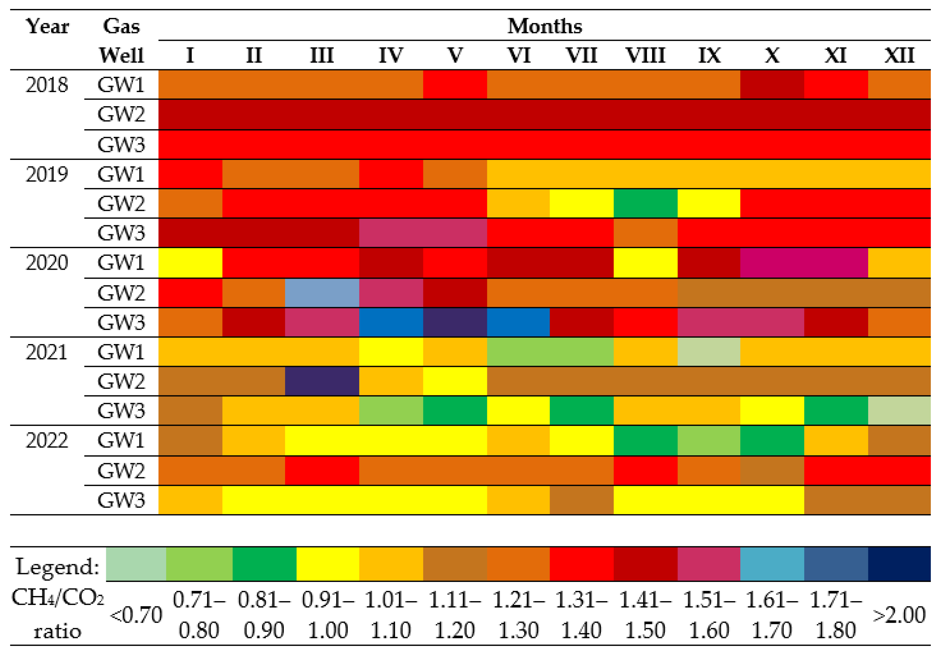
3.2. CH4/CO2 Volumetric Ratio

The CH4/CO2 volumetric ratio was calculated to provide an insight into the anaerobic reaction stage, i.e., the degree of CH4 oxidation into the deposited MSW in Cell-1 [47,74,81,89]. The CH4/CO2 ratio varied significantly among the gas wells, months, and years as follows: GW1 from 0.70, September 2021 to 1.54, November 2020; GW2 from 0.90, August 2019 to 2.01, March 2021 and GW3 from 0.68, December 2021 to 2.01, May 2020 (Figure 4). Despite variable results, predominantly higher values of that ratio (>1.24) were found in 2018, 2019, and 2020 (Phase 1—active cell, January 2018–June 2020) compared to 2021 and 2022 (<1.18) (Phase 2—closed cell, July 2020–December 2022). Exceptions to the general trend were observed during both periods: at GW1 (June–December) and at GW2 (June–September) in 2019, at GW1 (January, August and December) and at GW2 (September–December) in 2020 with lower values (0.90–1.15) than those during Phase 1 of Cell-1 as well as at GW2 (March) in 2021 and at GW2 for all months of 2022 with higher values (1.18–2.01) than those during Phase 2 of Cell-1. These contradictory results revealed the fragmented nature of organic waste biodegradation processes in the investigated cell by place and by time. Overall, the CH4/CO2 ratio for the three gas wells was greater than 1.0 throughout most of the monitoring period (GW1—92.78%, GW2—97.78% and GW3—92.22% of the time), indicating that the MSW in Cell-1 was still in the active phase of biomethanization [46]. Some authors noted that the CH4/CO2 ratio increases up to typical values (≥1.50) for a mature LFG [89]. The results obtained are logical, as newer waste typically has a CH4/CO2 ratio of about 1.5 and higher, as was found in this study in 2018 and most of the months in 2019 and 2020, while older waste (2021–2022) had a lower CH4/CO2 ratio as expected [74]. The results reported by other investigations of sites of different types, capacities, and age were within our results’ range: 1.53 [46], 1.00–1.50 [74], 0.7–2.2 [8], 0.69–0.76 [90]. In conclusion, the CH4/CO2 ratio in the present study demonstrates a great sensitivity and enables an accurate assessment of the methane phase of organic waste decomposition in different areas of the cell.

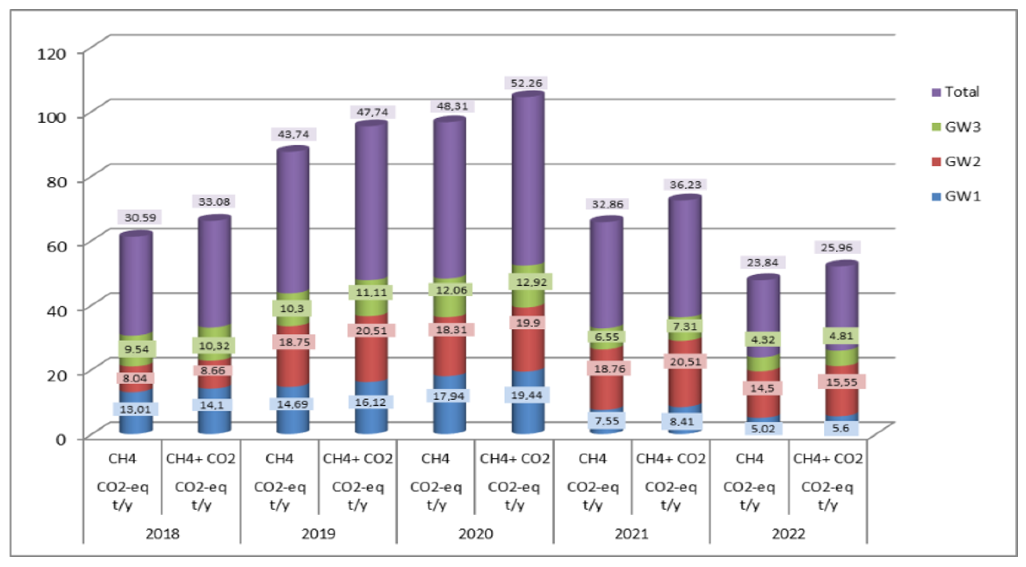
3.3. CH4 and CO2 Emissions

The results showed that the CO2 emissions were greater than CH4 emissions during the monitoring period and that their amount by gas wells and by years varied between 491.97 kg/y (GW3, 2022) and 1762.76 kg/y (GW2, 2019), and between 172.81 kg/y (GW3, 2022) and 750.41 kg/y (GW2, 2021), respectively (Table 5). Considering that the content of CH4, measured in volumetric percentages (% v/v), was greater than that of CO2 content (Table 3), the greater CO2 emission rates (kg) compared to those of CH4 could be explained by the differences in the mass of the two gases. The molecular mass of CO2 is 2.74 times greater than that of CH4 (44.01 vs. 16.04) and converting the values from volume percentages (% v/v) to mg/m3 resulted in higher values in mg/m3 with respect to CO2 emissions compared to those of CH4. Previous studies also reported that the CO2 emission rates are usually higher than the CH4 emission rates from landfills of different types [2,42]. The emissions of both gases demonstrated significant variability by gas wells both within the same year and among the different years of the observed period. On the whole, CH4 and CO2 emission rates by gas wells were higher in the winter period (December, January, and February) and in the first three months of the non-winter period (March, April, and May) compared to the last six months of the non-winter period (June–November).
According to the amount of the generated CH4 and CO2 emissions, the gas wells ranked differently during the individual years of the observed period. In 2018, the majority of CO2 and CH4 emissions were emitted from GW1, followed by GW3 and GW2, while in the remaining four years (2019–2022), the arrangement by gas wells was GW2 > GW1 > GW3. Although the spatial variability (according to the gas well location) in the emission of the two gases was very large, the quantity emitted from GW2 dominated over those from GW1 and GW3 (an exception was 2018), giving a reason to determine the zone of GW2 as a hotspot of Cell-1. Other researchers [91,92] have also identified hotspot areas of high CO2 and CH4 concentrations on MSW landfills, where the CO2 and CH4 hotspot areas have been very close.
The results for contradictory emission dynamics from the gas wells of the investigated landfill cell suggested that the factors influencing the CO2 and CH4 production were quite variable. Among those factors, the air temperature, atmospheric pressure, and precipitation could be highlighted. A relationship between meteorological factors and the topography of the terrain on which the landfill is located has also been reported [93]. In the literature, there are conflicting data about the influence of meteorological factors on LFG production. Some researchers found out that the LFG emission rates demonstrated a seasonal variability, with low values in summer and the highest values between September and May [94]; others reported the existence of a strong influence of atmospheric pressure on LFG CH4 concentration, LFG flow, and CH4 flow, while the ambient temperature was not a major meteorological parameter affecting LFG recovery [36]. The air temperature was not correlated with either CO2 or CH4 fluxes, despite the significant variation of that parameter [82,86]; whereas other data demonstrate that the LFG emissions generally increased as the average air temperature became higher [95]. CH4 emissions were commonly higher during colder temperatures in winter than during warm temperatures in summer [96]; the CH4 and CO2 emissions were the highest during the summer season, followed by the monsoon and the winter seasons [74,90] but LGE emissions did not show a significant difference between the end of the rainy period and the end of the dry period [92]. Therefore, it can be concluded that all these results reflect the specific conditions for each of the studied landfills.
Regarding the total annual CH4 and CO2 emissions, a general trend was observed. The emission of both gases increased from 2018 to 2020 (by 57.96% for CH4 and by 58.26% for CO2) when they reached the highest levels; afterwards, the emissions decreased to 2022 (by 50.65% for CH4 and by 46.36% for CO2) and attained the lowest levels. This divergent trend in the emissions of both gases could be explained by the different activities occurring in Cell-1 during the tested years. From January 2018 until the end of June 2020, Cell-1 was in operation and daily new amounts of MSW, including new amounts of organic matter, had been added. Therefore, during that phase there were conditions for the production of larger amounts of LFG, leading to an increase in CH4 and CO2 emissions. Previously reported data revealed that the exploitation parameters have a considerable influence on the emission of LFG in an operating landfill [97]. Another reason could be the high content of rapidly degradable organic carbon in MSW combined with high moisture content, which stimulates anaerobic degradation, i.e., the production of more LFG within a short period [98]. After June 2020, Cell-1 was closed as its capacity was reached and it was temporarily covered by native soil. The discontinuation of MSW disposal in the cell led to the depletion of the organic matter reserves and, accordingly, to a decrease in the emission rates of both gases until the end of 2022. These results are in the line with previous studies reporting that operational landfills emit more LFG/CH4 than closed landfills, since the major part of degradation occurs in the first few years following MSW disposal (during the active phase of the landfills) with emission rates decreasing with time after their closure (during the closed phase of the landfills) [50,98]. Other researchers [23,26,38,42] pointed out that, after landfill closure, LFG/methane generation decreases and the process usually lasts many years. Our results are distinguished from those of other authors by the high rates of growth (>57–58%) and the decrease (<46–50%) in CH4 and CO2 emissions, respectively, during the active and closed phases of the cell, each of them lasting 2.5 years. The probable reasons for this phenomenon are multiple and different but are most likely related to the amount of deposited MSW, the content of MSW organic matter, and the thickness of the deposited waste as well as the environmental conditions (atmospheric pressure, temperature, moisture, pH, microbial activities, etc.). The monitored landfill cell has a relatively small capacity (292,254 t) and a small thickness of the deposited MSW (1.80 m), while in other studies the capacity of the landfills and the thickness of the deposited MSW were much greater; therefore, the produced CH4 and CO2 levels were also much higher than in the present study [36,66,83,99,100,101,102]. Some authors reported that the changes in the quantity of waste affected the annual methane production from the landfill more than the changes of waste composition [103].
The CH4 and CO2 emissions from Cell-1, presented as equivalent amounts of carbon dioxide (CO2-eq), exhibited the same dynamics over the years of the monitoring period as did the individual emissions of both gases. Carbon footprint calculations showed that, for the five tested years, the three gas wells of Cell-1 emitted between 25.96 t CO2-eq/y (2022) and 52.26 t CO2-eq/y (2020), see Figure 5. It turned out that the three gas wells had different contributions to those quantities: the greatest contribution was made by GW2, followed by GW1 and GW3. The annually emitted amounts of CO2-eq from all gas wells of Cell-1 were relatively small but were multiplied for the cells of all 53 landfills in Bulgaria; therefore, the picture was dramatically different. That is why, no matter how insignificant these amounts are, an environmentally friendly solution for their reduction and utilization must be sought. Due to the low profitability of energy production from LFG (methane) produced by the investigated cell, the plan for the management of generated biogas in cells/landfills after their reclamation includes gathering and flaring LFG from all wells in a common duct.

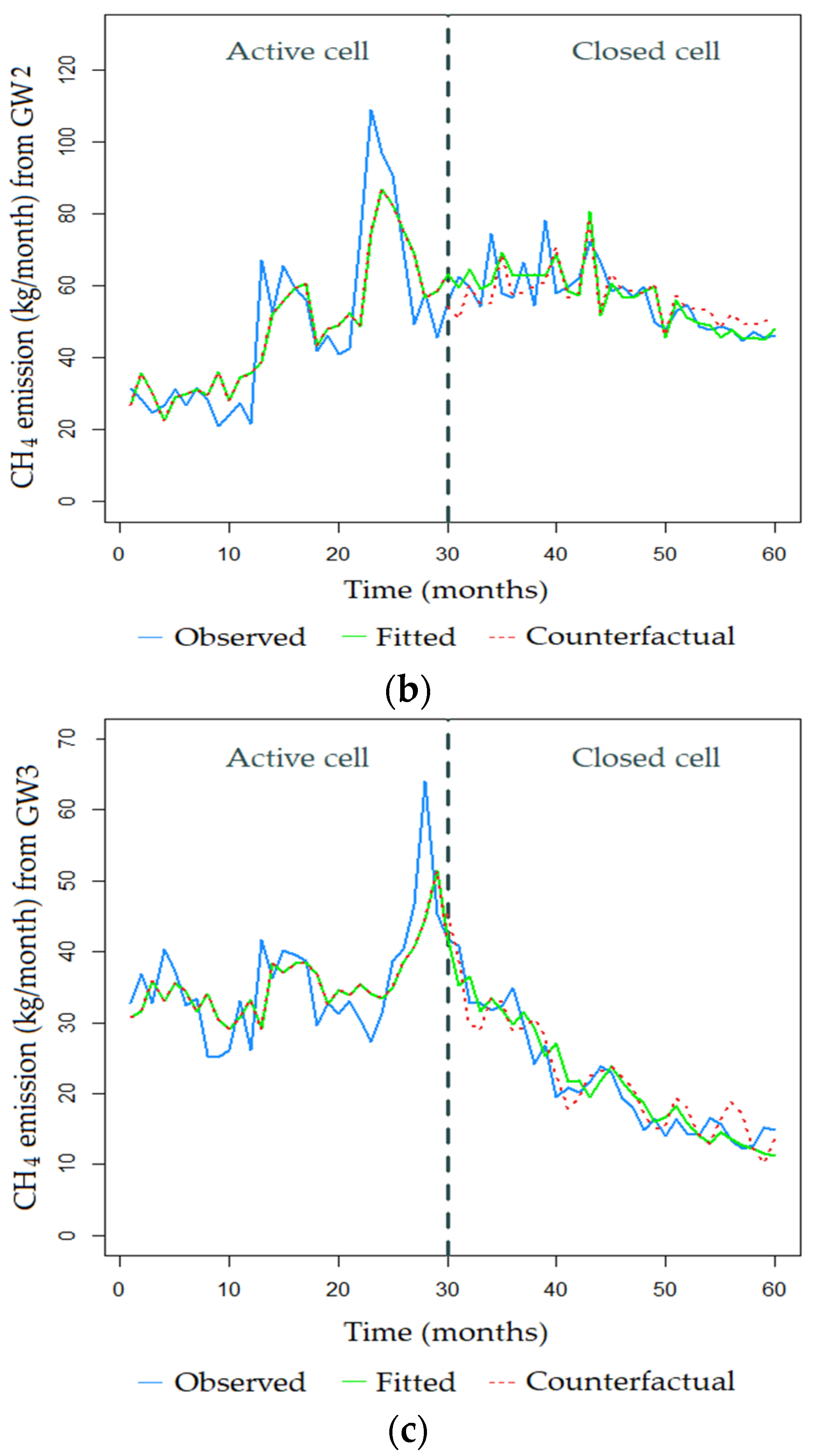
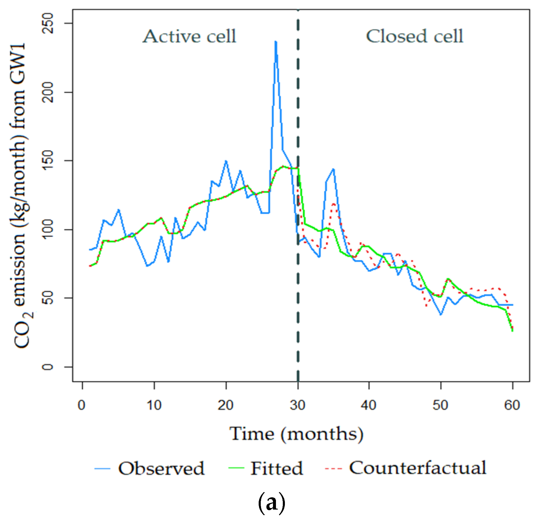
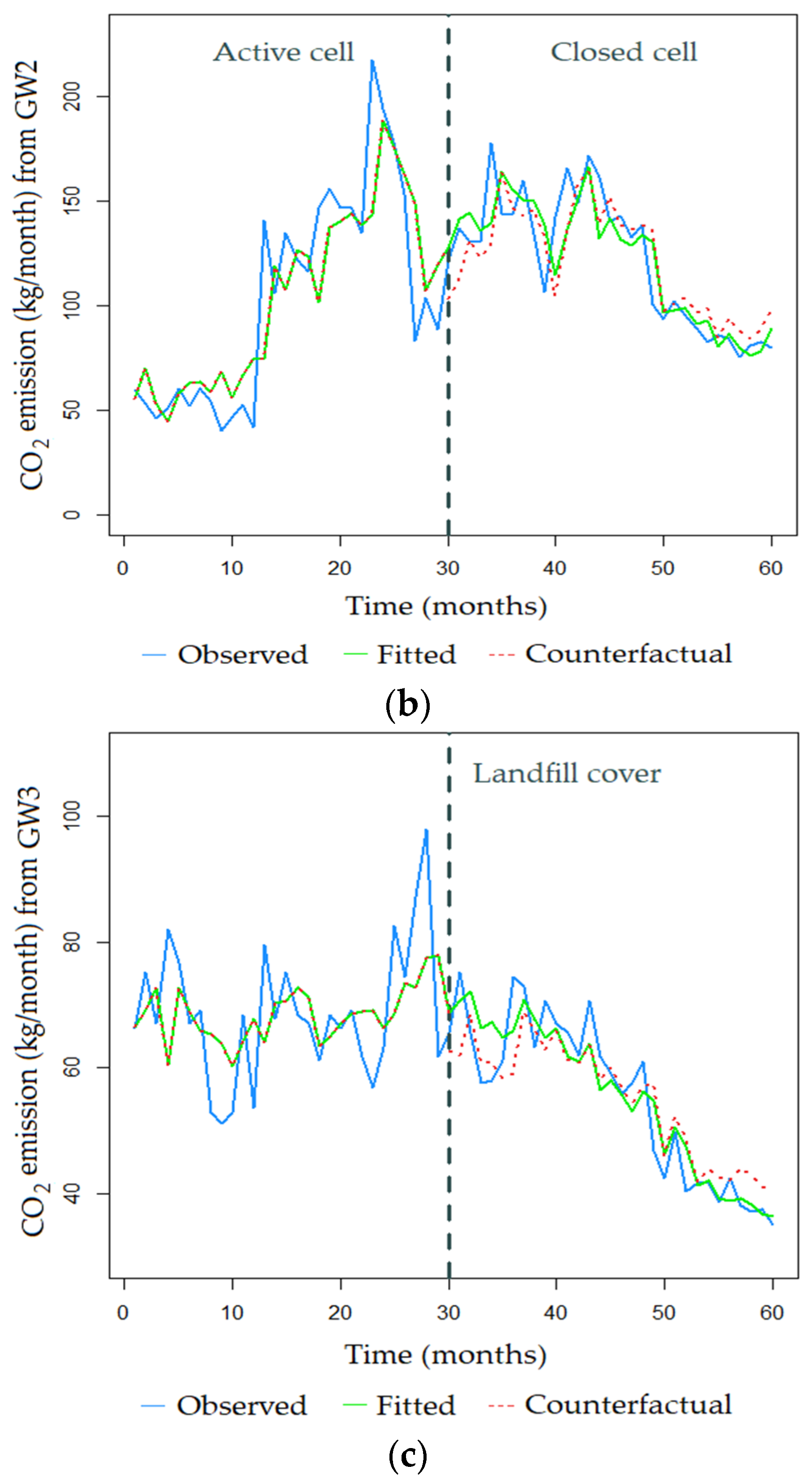
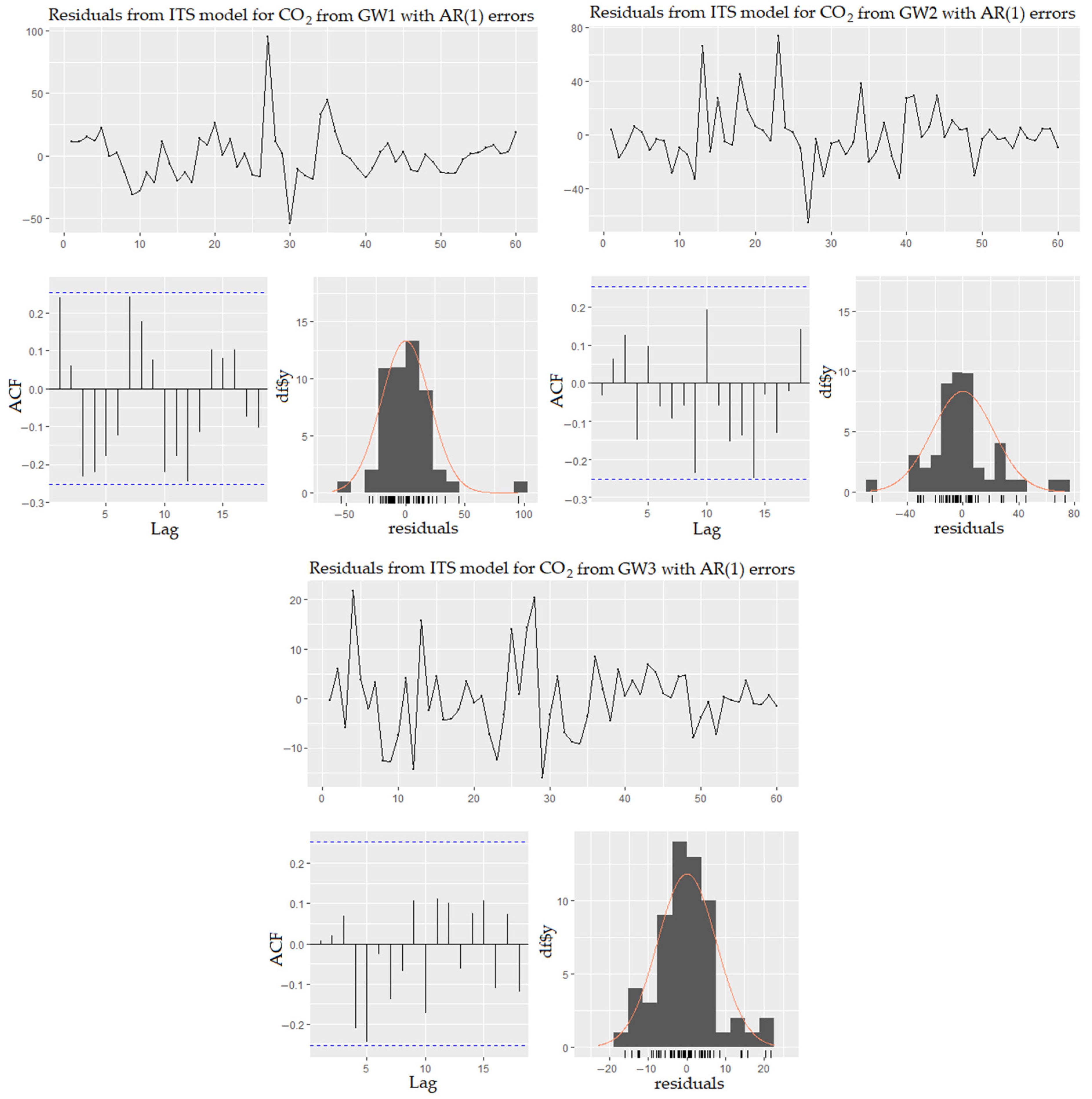
3.4. Interrupted Time Series ARMA Model Analysis

Table 6 presents the results of the descriptive statistics of the variables. Regarding the gas wells, the CH4 and CO2 emissions from GW2 had the highest mean values of 52.237 and 112.849, respectively, while the CH4 and CO2 emissions from GW3 had the lowest mean values of 28.560 and 61.779, respectively. The highest mean values of atmospheric pressure and air temperature were found at GW3—988.093 and 18.192, respectively—while the lowest were computed at GW1—987.453 and 17.783, respectively. The mean value of the precipitation was 34.538.
The skewness of data for all gas wells was positive for CH4 and CO2 (except for CO2 from GW3) and negative for the atmospheric pressure and air temperature. The highest values of 1.150 for CH4 and 1.196 for CO2 were for GW1, meaning that the data were skewed to the right. With regard to atmospheric pressure and air temperature, the lowest values of −1.323 and −0.179 were found at GW3. The skewness value for precipitation was positive (1.179). In assessing the kurtosis of the CH4 and CO2 datasets, the emissions had the highest values of 2.185 and 2.933 for GW1, respectively, while the lowest values were 0.548 for GW3 and −0.789 for GW2, respectively. The highest values were 3.701 for the atmospheric pressure of GW3 and −0.981 for the air temperature of GW1, while the lowest values were 3.587 for the atmospheric pressure of GW1 and −1.048 for the air temperature of GW3, respectively. The kurtosis value of precipitation was 0.484.
The Jarque–Bera test failed to reject the H0 hypothesis that the data were normally distributed in all variables, excluding the CH4 and CO2 from GW1, atmospheric pressure from all gas wells, and precipitation—the Jarque–Bera statistic was positive with a p-value of more than 0.05. Nevertheless, we can conclude that residuals of all variables were approximately normally distributed, as the skewness was between −2 and +2 and kurtosis was between −7 and +7 [104,105]. Normality is a desirable characteristic for the data analysis required.
Table 7 and Table 8 present the estimates of α and β parameters and corresponding p-values for the obtained ITS models implemented for CH4 and CO2 emissions from each gas well. In the case of an empty cell, meaning that the corresponding coefficient was not significantly different from zero, it was removed from the model. Besides the covariate coefficients β, the following parameters were estimated: the intercept α0, the baseline trend slope α1, and the post-closed Cell-1 level (trend slope) change α23), which are represented in Equation (1). Specifically, α0 + α2 + Xtβ and α1 + α3 described the level and the trend slope after the Cell-1 closure, to be compared with α0 + Xtβ and α1, respectively.
It can be noted that precipitation had no significant effect on CH4 and CO2 emissions, thus it was excluded from all models. The most important meteorological variable was the atmospheric pressure with a significant positive effect for CH4 (from GW1 and GW2) and CO2 (from GW1) emissions, and a negative effect for the emissions of both gases from GW2. Air temperature had a significant, negative effect for CH4 (from GW2) and CO2 (from GW3) emissions. The dummy variable related to the non-winter effect was significantly different from zero for the emissions of both gases, only from GW1 located at the top of the cell in the area last filled up with MSW and last covered with a temporary layer of soil (Figure 2).
Parameter α1 indicates the air pollution trend before Cell-1 closure. It was significantly positive for CH4 (from GW2) and CO2 (from GW1 and GW2) emissions. This was perhaps associated with the approach of warmer weather and sunny days. For each passing day, the air pollution with CH4 (from GW2) increased by 1.820 points whereas that of CO2 (at GW1 and GW2) increased by 2.124 and 4.034 points, respectively. These trends were also evident from the observed time series represented in Figure 6 and Figure 7.
The α2 coefficient indicates the air pollution immediately after Cell-1 closure. Its immediate effect was negative and significant only for CO2 emissions from GW1. This result makes sense, since the decrease was not expected to be very high immediately after Cell-1 closure. In this regard, some authors reported that LFG emissions peak a year after the closure of a landfill [42].
The α3 coefficient indicates how the trend changed after Cell-1 closure. The sustained effect was negative and significant for CH4 and CO2 emissions from all gas wells. Therefore, for each day after the Cell-1 closure, the air pollution of CH4 decreased by −1.997 (from GW1), −2.576 (from GW2), and −1.153 (from GW3) points, respectively. For each passing day, the air pollution of CO2 decreased by −4.469 (from GW1), −6.986 (from GW2), and −1.558 (from GW3) points, respectively. In previous studies, many researchers pointed out the same trends in the reduction of CH4 and CO2 emissions after landfill closure [23,26,42,50].
The results obtained are confirmed by the graphs on Figure 6 and Figure 7, where the observed and fitted (using the estimated parameters presented in Table 7 and Table 8) time series are presented together with the counterfactual predictions. The latter represent the expected time series in the hypothetical scenario under which the Cell-1 was not still closed, i.e., with no intervention and assuming that the time series was stationary after accounting for time-varying confounders.
Figure 6 and Figure 7 demonstrate an increase in the observed values between October and December 2020, i.e., immediately after Cell-1 closure, which may be related to the specific meteorological conditions in the area during that period, characterized by an abundance of precipitation (34.3% of total annual precipitation) and relatively high air temperatures (especially in October (20.2 °C) and November (17.1 °C). In December, the air temperature was lower (6.1 °C), as well as covering the Cell-1 with a layer of soil. The surface layer of soil limits the access of oxygen and favors the anaerobic degradation of waste organic matter. Moreover, the higher water content of the substrate acts as a diffusion barrier for the methane and oxygen that can be utilized by the oxidizing bacteria, thereby leading to increased emissions. In addition, the higher air temperatures positively affected both methane production and oxidation as these were temperature-dependent microbial processes [94]. Another study also found that CH4 and CO2 emissions during the wet season were approximately 1.5 times higher compared to during the dry season as higher moisture content facilitated nutrient transportation through waste layers and accelerated waste decomposition to produce more LFG [86].
Table 9 presents the estimates of the ARMA coefficients. Time series were characterized by the following temporal dynamics: an MA(2) structure was estimated for CH4 from GW1, while an AR(1) was the best choice for CH4 from GW2 and GW3, and for CO2 from all gas wells.
Figure 8 and Figure 9 show the time plots, the ACF plots, and the histogram of the residuals from the ARMA models. The time plots show some variation over time but are otherwise relatively unremarkable. The histograms suggest that the residuals are normally distributed. The ACF plots of the residuals show that all autocorrelations were within the threshold limits. Therefore, we concluded that the residuals behaved similarly to white noise. A Ljung–Box test returned the following statistic and p-value for the residuals from CH4 ARMA models: 17.566 (p-value = 0.541), 21.038 (p-value = 0.103), and 15.585 (p-value = 0.138), respectively; and from CO2 ARMA models: 25.729 (p-value = 0.187), 13.643 (p-value = 0.343), and 14.360 (p-value = 0.245), respectively. These large p-values suggested that the residuals were white noise. The correlations between predicted and observed values from obtained ARMA models were strong, positive, and ranged from 0.739 to 0.896.
Future investigations of landfills, using the Interrupted Time Series ARMA model could reveal the local differences and point out the relevant factors affecting the dynamics of CH4 and CO2 emissions during active (before cover) and closed (after cover) phases of the landfills. That knowledge will contribute to forming effective LFG emissions management policies, aimed at air quality improvement and human health protection.

4. Conclusions

The management of greenhouse gas emissions from MSW landfills is of great importance in seeking solutions to reduce their impact on global warming and the Earth’s climate. In Bulgaria, 53 landfills for non-hazardous MSW waste are currently in operation, so the study of the processes generating greenhouse gas emissions from them will contribute to the formation of an adequate policy and the implementation of environmentally friendly solutions for the sustainable management of the landfills. This study was the first of its kind in the country to assess the CH4 and CO2 emissions from three gas wells (GW1, GW2, and GW3) of a landfill cell (Cell-1) during the active and closed phases (2.5 years duration for each of them) of a regional non-hazardous waste landfill—Harmanli—based on in situ measurement of the concentrations of the two gases.
The results show that the CH4 and CO2 concentrations varied widely by gas wells, months, and years (2.06–15.1% v/v). During most of the monitored period, the CH4 values of gas wells were 1.14–1.54 times higher than the CO2 values but opposite results were also observed, although less often and to a lesser extent. The monthly CH4 and CO2 concentrations by gas wells across individual years varied within narrower limits than among individual gas wells within the same year, which determines the month within a year as a factor with a greater impact on the concentration of both gases than the factor year. From 2018 to 2022, the concentrations of the produced LFG decreased, especially after the Cell-1 closure in June 2020, by 43.6% for CH4 and 38.4% for CO2 on average, indicating the rapid biodegradation of the deposited waste. The results obtained for the two gases were significantly lower than those cited in this paper, which may be affected by many factors, two of which are of key importance—the amount of MSW deposited in the landfill and the content of organic matter in the deposited waste. With respect to both parameters, the studied landfill cell ranks below the landfills from other studies.
The CH4/CO2 volumetric ratio values reflect the biodegradation (methanogenesis) of the deposited waste. The parameters demonstrate high variability by gas wells, months, and years (0.68–2.01), which made it a suitable indicator for assessing the level of the methane phase of organic waste decomposition in different areas of the cell. Predominantly higher values of that ratio were established during Phase 1—active cell (>1.24) compared to Phase 2—closed cell (<1.18). This is logical and corresponds with the results for CH4 and CO2 concentrations and emissions.
The CO2 emissions from all GWs were greater than the CH4 emissions and could be explained by the differences in the masses of the two gases (44.01 vs. 16.04). The conversion of the values from volumetric percentages (% v/v) to mg/m3 resulted in higher values in mg/m3, i.e., in kg/y for CO2, compared to those of CH4 emissions. The emissions of both gases demonstrated significant variability by gas wells, months, and years but, on the whole, the emission rates by gas wells were higher in the colder months (December–February) and partly in spring (March–May) compared to the warmer months of the year (June–November). Despite the spatial variability of the emissions in the zones of the three GWs, the quantity emitted from GW2 dominated over that from GW1 and GW3, giving a reason to determine the GW2 zone as a hotspot of Cell-1. A general trend of change in the emissions of the two gases was observed—during the active phase of the Cell-1, the emissions drastically increased by about 58% and, after the Cell-1 closure, they drastically decreased by 46–50%. This phenomenon can be explained by the different activities and the different processes that take place in the cell. During the active cell, daily new amounts of MSW are added, including new amounts of organic matter, which stimulate the generation of gas emissions. Closing the cell stops this activity and, as a result, the organic matter in the waste is decomposed and emissions decrease. The high rates of increase and decrease of the emissions are probably due to the relatively small amount of the deposited MSW as well as the specific environmental conditions in the area of Cell-1. The CH4 and CO2 emissions, presented as equivalent amounts of carbon dioxide (CO2-eq), show that, for the five tested years, the three gas wells of Cell-1 emitted between 25.96 t CO2-eq/y and 52.26 t CO2-eq/y. The emitted amounts are relatively small and the production of energy from such quantities is not profitable. Therefore, flaring of the generated biogas is performed.
Finally, the results obtained from the Interrupted Time Series ARMA model (after adjusting for some meteorological factors and the non-winter effect) confirmed the negative and significant effect on CH4 and CO2 emissions immediately after the closure of Cell-1, with the exception of the CO2 emissions from GW1. The correlations between the predicted and observed values obtained by the ARMA model were strong, positive, and ranged from 0.739 to 0.896. The Interrupted Time Series ARMA model was shown to be suitable for use in similar investigations. Therefore, the main findings of this research may become an important part of further deeper investigations and the analysis of the LFG emitted by landfills in Bulgaria.

Author Contributions

Conceptualization, G.P., G.K., M.I. and D.B.; methodology, G.K., G.P., L.D., M.I. and D.D.; software, M.I. and L.D.; validation, G.P., D.B. and G.B.; formal analysis, G.K., G.P., L.D. and M.I.; investigation, D.B., D.D. and G.K.; resources, D.B., D.D. and L.D.; data curation, G.P., G.K., L.D. and M.I.; writing—original draft preparation, G.P. and L.D.; writing—review and editing, G.P., G.K., D.B., L.D. and M.I.; visualization, G.P., D.B. and M.I.; supervision, G.P., G.K., L.D. and M.I.; project administration, D.B. and G.B.; funding acquisition, G.B., L.D. and D.D. All authors have read and agreed to the published version of the manuscript.

Funding

This research was supported by the Bulgarian Ministry of Education and Science under the National Research Program “Smart crop production” approved by Decision of the Ministry Council #866/26.11.2020.

Institutional Review Board Statement

Not applicable.

Informed Consent Statement

Not applicable.

Data Availability Statement

Not applicable.

Acknowledgments

The authors are grateful to Harmanli City Council and the management team of Ekoresurs Harmanli Ltd.—Regional non-hazardous waste landfill and National Program for Research “Young Scientists and Postdoctoral Students” for the help during the performance of this experiment.

Conflicts of Interest

The authors declare no conflict of interest.

Abbreviations

MSWmunicipal solid waste
GHGgreenhouse gas
LFGlandfill gas
GWgas well
EUEuropean Union
RNHWLregional non-hazardous waste landfill
HDPEhigh-density polyethylene
ITSInterrupted Time Series
NWMPNational Waste Management Plan
BDSBulgarian State Standard
CvCoefficients of variation.

References

  1. Hannan, M.A.; Abdulla Al Mamun, M.; Hussain, A.; Basri, H.; Begum, R.A. A review on technologies and their usage in solid waste monitoring and management systems: Issues and challenges. Waste Manag. 2015, 43, 509–523. [Google Scholar] [CrossRef] [PubMed]
  2. Njoku, P.O.; Odiyo, J.O.; Durowoju, O.S.; Edokpayi, J.N. A Review of Landfill Gas Generation and Utilisation in Africa. Open Environ. Sci. 2018, 10, 1–15. [Google Scholar] [CrossRef] [Green Version]
  3. Duan, Z.; Scheutz, C.; Kjeldsen, P. Trace gas emissions from municipal solid waste landfills: A review. Waste Manag. 2021, 119, 39–62. [Google Scholar] [CrossRef]
  4. Hoornweg, D.A.; Bhada-Tata, P. What a Waste: A Global Review of Solid Waste Management; Urban Development Series; Knowledge Papers No. 15; World Bank: Washington, DC, USA, 2012; Available online: https://openknowledge.worldbank.org/handle/10986/17388 (accessed on 20 April 2022).
  5. Kaza, S.; Yao, L.; Bhada-Tata, P.; Van Woerden, F. At a Glance: A Global Picture of Solid Waste Management. In What a Waste 2.0: A Global Snapshot of Solid Waste Management to 2050; Kaza, S., Yao, L., Bhada-Tata, P., Van Woerden, F., Eds.; World Bank Report; World Bank: Washington, DC, USA, 2018; pp. 17–38. Available online: http://hdl.handle.net/10986/30317 (accessed on 20 September 2022).
  6. Ricci-Jürgensen, M.; Gilbert, J.; Ramola, A. Global Assessment of Municipal Organic Waste Production and Recycling; International Solid Waste Association (ISWA): Rotterdam, The Netherlands, 2020; pp. 6–7. Available online: https://www.altereko.it/wp-content/uploads/2020/03/Report-1-Global-Assessment-of-Municipal-Organic-Waste.pdf (accessed on 9 December 2021).
  7. Stanisavljević, N.; Ubavin, D.; Batinić, B.; Johann Fellner, J.; Vujić, G. Methane emissions from landfills in Serbia and potential mitigation strategies: A case study. Waste Manag. Res. 2012, 30, 1095–1103. [Google Scholar] [CrossRef] [PubMed]
  8. Yang, L.; Chen, Z.; Zhang, X.; Liu, Y.; Xie, Y. Comparison study of landfill gas emissions from subtropical landfill with various phases: A case study in Wuhan, China. J. Air Waste Manag. Assoc. 2015, 65, 980–986. [Google Scholar] [CrossRef] [PubMed]
  9. Ferronato, N.; Torretta, V. Waste mismanagement in developing countries: A review of global issues. Int. J. Environ. Res. Public Health 2019, 16, 1060. [Google Scholar] [CrossRef] [PubMed] [Green Version]
  10. Vaverková, M.D. Landfill Impacts on the Environment—Review. Geosciences 2019, 9, 431. [Google Scholar] [CrossRef] [Green Version]
  11. Zhang, C.; Xu, T.; Feng, H.; Chen, S. Greenhouse Gas Emissions from Landfills: A Review and Bibliometric Analysis. Sustainability 2019, 11, 2282. [Google Scholar] [CrossRef] [Green Version]
  12. Fischedick, M.; Roy, J.; Abdel-Aziz, A.; Acquaye, A.; Allwood, J.; Ceron, J.P.; Geng, Y.; Kheshgi, H.; Lanza, A.; Perczyk, D.; et al. Industry. In Climate Change 2014: Mitigation of Climate Change. Contribution of Working Group III to the Fifth Assessment Report of the Intergovernmental Panel on Climate Change; Edenhofer, O., Pichs-Madruga, R., Sokona, Y., Farahani, E., Kadner, S., Seyboth, K., Adler, A., Baum, I., Brunner, S., Eickemeier, P., et al., Eds.; Cambridge University Press: Cambridge, UK; New York, NY, USA, 2014; pp. 743–784. Available online: http://www.ipcc.ch/report/ar5/wg3/ (accessed on 15 December 2022).
  13. Wang, Y.; Levis, J.W.; Barlaz, M.A. An Assessment of the Dynamic Global Warming Impact Associated with Long-Term Emissions from Landfills. Environ. Sci. Technol. 2020, 54, 1304–1313. [Google Scholar] [CrossRef]
  14. Paraskaki, I.; Lazaridis, M. Quantification of landfill emissions to air: A case study of the Ano Liosia landfill site in the greater Athens area. Waste Manag. Res. 2005, 23, 199–208. [Google Scholar] [CrossRef]
  15. Aderemi, A.O.; Falade, T.C. Environmental and health concerns associated with the open dumping of municipal solid waste: A Lagos, Nigeria experience. Am. J. Environ. Eng. 2012, 2, 160–165. [Google Scholar] [CrossRef] [Green Version]
  16. Palmiotto, M.; Fattore, E.; Paiano, V.; Celeste, G.; Colombo, A.; Davoli, E. Influence of a municipal solid waste landfill in the surrounding environment: Toxicological risk and odor nuisance effects. Environ. Int. 2014, 68, 16–24. [Google Scholar] [CrossRef] [PubMed]
  17. Maheshwari, R.; Gupta, S.; Das, K. Impact of landfill waste on health: An overview. IOSR J. Environ. Sci. Toxicol. Food. Technol. (IOSR-JESTFT) 2015, 1, 17–23. Available online: https://www.iosrjournals.org/iosr-jestft/papers/SSSSMHB/Volume-4/4.paper%2053.pdf (accessed on 15 June 2022).
  18. Njoku, P.O.; Edokpayi, J.N.; Odiyo, J.O. Health and Environmental Risks of Residents Living Close to a Landfill: A Case Study of Thohoyandou Landfill, Limpopo Province, South Africa. Int. J. Environ. Res. Public Health 2019, 16, 2125. [Google Scholar] [CrossRef] [PubMed] [Green Version]
  19. Sallam, R.M.A. Landfill emissions and their impact on the environment. Int. J. Chem. Stud. 2020, 8, 1567–1574. [Google Scholar] [CrossRef]
  20. Siddiqua, A.; Hahladakis, J.N.; Al-Attiya, W.A.K.A. An overview of the environmental pollution and health effects associated with waste landfilling and open dumping. Environ. Sci. Pollut. Res. 2022, 29, 58514–58536. [Google Scholar] [CrossRef]
  21. Polvara, E.; Essna ashari, B.; Capelli, L.; Sironi, S. Evaluation of Occupational Exposure Risk for Employees Working in Dynamic Olfactometry: Focus on Non-Carcinogenic Effects Correlated with Exposure to Landfill Emissions. Atmosphere 2021, 12, 1325. [Google Scholar] [CrossRef]
  22. Durlević, U.; Novković, I.; Carević, I.; Valjarević, D.; Marjanović, A.; Batoćanin, N.; Krstić, F.; Stojanović, L.; Valjarević, A. Sanitary landfill site selection using GIS-based on a fuzzy multi-criteria evaluation technique: A case study of the City of Kraljevo, Serbia. Environ. Sci. Pollut. Res. 2023, 30, 37961–37980. [Google Scholar] [CrossRef]
  23. Niskanen, A.; Värri, H.; Havukainen, J.; Uusitalo, V.; Horttanainen, M. Enhancing landfill gas recovery. J. Clean. Prod. 2013, 55, 67–71. [Google Scholar] [CrossRef]
  24. Yang, D.; Xu, L.; Gao, X.; Guo, Q.; Huang, N. Inventories and reduction scenarios of urban waste-related greenhouse gas emissions for management potential. Sci. Total Environ. 2018, 626, 727–736. [Google Scholar] [CrossRef] [PubMed]
  25. Khatiwada, D.; Golzar, F.; Mainali, B.; Devendran, A.A. Circularity in the Management of Municipal Solid Waste: A Systematic Review. Environ. Clim. Technol. 2021, 25, 491–507. [Google Scholar] [CrossRef]
  26. Guo, H.; Xu, H.; Liu, J.; Nie, X.; Li, X.; Shu, T.; Bai, B.; Ma, X.; Yao, Y. Greenhouse Gas Emissions in the Process of Landfill Disposal in China. Energies 2022, 15, 6711. [Google Scholar] [CrossRef]
  27. Intergovernmental Panel on Climate Change (IPCC). Chapter 3: Solid Waste Disposal. In 2006 IPCC Guidelines for National Greenhouse Gas Inventories—Waste; Institute for Global Environmental Strategies (IGES): Hayama, Japan, 2006; Volume 5, pp. 8–40. Available online: https://www.ipcc-nggip.iges.or.jp/public/2006gl/vol5.html (accessed on 2 March 2023).
  28. Pecorini, I.; Iannelli, R. Landfill GHG Reduction through Different Microbial Methane Oxidation Biocovers. Processes 2020, 8, 591. [Google Scholar] [CrossRef]
  29. Scheutz, C.; Kjeldsen, P.; Bogner, J.E.; De Visscher, A.; Gebert, G.; Hilger, H.A.; Huber-Humer, M.; Spokas, K. Microbial methane oxidation processes and technologies for mitigation of landfill gas emissions. Waste Manag. Res. 2009, 27, 409–455. [Google Scholar] [CrossRef] [PubMed]
  30. United Nations Environment Programme (UNEP). Waste and Climate Change—Global Trends and Strategy Framework, USA. 2010. Available online: https://wedocs.unep.org/20.500.11822/8648 (accessed on 19 March 2023).
  31. Brindley, T. The Management of Landfill Gas. In Landfill Gas—Industry Code of Practice; Environment Services Association; Todeka Ltd.: Codicote, UK, 2012; Available online: https://www.esauk.org/application/files/8515/5782/4933/20120301_ICoP_Landfill_Gas_2012.pdf (accessed on 1 March 2023).
  32. Mohsen, R.A. Estimation of Greenhouse Gas Emissions in Municipal Solid Waste Landfills in Ontario Using Mathematical Models and Direct Measurements. Ph.D. Thesis, University of Guelph, Guelph, ON, Canada, December 2019; pp. 4–16. Available online: https://atrium.lib.uoguelph.ca/xmlui/bitstream/handle/10214/17659/AMohsen_Riham_201912_phd.pdf?sequence=3 (accessed on 10 February 2023).
  33. Asgari, M.; Safavi, K.; Mortazaeinezahad, F. Landfill Biogas production process. In Proceedings of the International Conference on Food Engineering and Biotechnology (IPCBEE), Bangkok, Thailand, 7–9 May 2011; IACSIT Press: Singapore, 2011; Volume 9, pp. 208–212. [Google Scholar] [CrossRef]
  34. Ciuła, J.; Kozik, V.; Generowicz, A.; Gaska, K.; Bąk, A.; Paździor, M.; Barbusiński, K. Emission and neutralization of methane from a municipal landfill-parametric analysis. Energies 2020, 13, 6254. [Google Scholar] [CrossRef]
  35. Haeming, H.; Bretthauer, F.; Heyer, K.-U.; Stegmann, R.; Quicker, P. Waste, 8. Landfilling and Deposition. In Ullmann’s Encyclopedia of Industrial Chemistry; Wiley: Hoboken, NJ, USA, 2021. [Google Scholar] [CrossRef]
  36. Aghdam, E.F.; Scheutz, C.; Kjeldsen, P. Impact of meteorological parameters on extracted landfill gas composition and flow. Waste Manag. 2019, 87, 905–914. [Google Scholar] [CrossRef] [Green Version]
  37. Pehme, K.-M.; Orupõld, K.; Kuusemets, V.; Tamm, O.; Jani, Y.; Tamm, T.; Kriipsalu, M. Field Study on the Efficiency of a Methane Degradation Layer Composed of Fine Fraction Soil from Landfill Mining. Sustainability 2020, 12, 6209. [Google Scholar] [CrossRef]
  38. Chen, C.; Hegde, U.; Chang, C.-H.; Yang, S.-S. Methane and carbon dioxide emissions from closed landfill in Taiwan. Chemosphere 2008, 70, 1484–1491. [Google Scholar] [CrossRef]
  39. Capelli, L.; Sironi, S.; Del, R.; Rosso, R.D.; Magnano, E. Evaluation of landfill surface emissions. Chem. Eng. Trans. 2014, 40, 187–192. [Google Scholar] [CrossRef]
  40. US Environmental Protection Agency. Basic Information about Landfill Gas; USEPA: Washington, DC, USA, 2023. Available online: https://www.epa.gov/lmop/basic-information-about-landfill-gas (accessed on 25 March 2023).
  41. Bhowmik, D. Global methane emission: Patterns and Kuznets hypothesis. AU eJournal of Interdiscipl. Res. 2020, 5, 22–43. Available online: http://www.assumptionjournal.au.edu/index.php/eJIR/article/view/4792 (accessed on 7 July 2020).
  42. Njoku, P.O.; Edokpayi, J.N. Estimation of landfill gas production and potential utilization in a South Africa landfill. J. Air Waste Manag. Assoc. 2022, 73, 1–14. [Google Scholar] [CrossRef]
  43. Glöser-Chahoud, S. Methane emissions and related abatement technologies from waste landfills and the natural gas grid in Europe. In Proceedings of the Joint EECCA_CG-TFTEI Virtual Workshop, Online, 26–27 April 2021; French-German Institute for Environmental Research (DFIU/KIT): Karlsruhe, Germany, 2021; pp. 1–27. Available online: https://unece.org/sites/default/files/2021-04/Methane%2027.04.pdf (accessed on 15 April 2023).
  44. Olaguer, E.P.; Jeltema, S.; Gauthier, T.; Jermalowicz, D.; Ostaszewski, A.; Batterman, S.; Xia, T.; Raneses, J.; Kovalchick, M.; Miller, S.; et al. Landfill Emissions of Methane Inferred from Unmanned Aerial Vehicle and Mobile Ground Measurements. Atmosphere 2022, 13, 983. [Google Scholar] [CrossRef]
  45. European Environmental Agency (EEA). Methane Emissions in the EU: The Key to Immediate Action on Climate Change. 2023. Available online: https://www.eea.europa.eu/publications/methane-emissions-in-the-eu (accessed on 30 November 2022).
  46. Hamoda, M.F. Air Pollutants Emissions from Waste Treatment and Disposal Facilities. J. Environ. Sci. Health Part A 2006, 41, 77–85. [Google Scholar] [CrossRef] [PubMed]
  47. Pratt, C.; Walcroft, A.S.; Deslippe, J.; Tate, K.R. CH4/CO2 ratios indicate highly efficient methane oxidation by a pumice landfill cover-soil. Waste Manag. 2013, 33, 412–419. [Google Scholar] [CrossRef] [PubMed]
  48. Abualqumboz, M.S.; Malakahmad, A.; Mohammed, N.I. Greenhouse gas emissions estimation from proposed El Fukhary Landfill in the Gaza Strip. J. Air Waste Manag. Assoc. 2016, 66, 597–608. [Google Scholar] [CrossRef] [Green Version]
  49. Barlaz, M.A.; Chanton, J.P.; Green, R.B. Controls on landfill gas collection efficiency: Instantaneous and lifetime performance. J. Air Waste Manag. Assoc. 2009, 59, 1399–1404. [Google Scholar] [CrossRef] [PubMed] [Green Version]
  50. Chalvatzaki, E.; Lazaridis, M. Estimation of greenhouse gas emissions from landfills: Application to the Akrotiri landfill site (Chania, Greece). Global NEST J. 2010, 12, 108–116. Available online: https://journal.gnest.org/sites/default/files/Journal%20Papers/108-116_681_Lazaridis_12-1.pdf (accessed on 11 February 2022).
  51. Gupta, J.; Ghosh, P.; Kumari, M.; Thakur, I.S.; Swati. Chapter 14: Solid waste landfill sites for the mitigation of greenhouse gases. In Biomass, Biofuels, Biochemicals—Climate Change Mitigation: Sequestration of Green House Gases; Thakur, I.S., Pandey, A., Ngo, H.H., Larroche, C., Eds.; Elsevier: Amsterdam, The Netherlands, 2022; pp. 315–340. [Google Scholar] [CrossRef]
  52. European Environment Agency (EEA). Annual European Union Greenhouse Gas Inventory 1990–2020 and Inventory Report. 2022. Available online: https://www.eea.europa.eu/publications/annual-european-union-greenhouse-gas-1 (accessed on 31 May 2022).
  53. European Environmental Agency (EEA). Municipal Waste Management across European Countries—Briefing. 2022. Available online: https://www.eea.europa.eu/publications/municipal-waste-management-across-european-countries (accessed on 14 November 2022).
  54. Eurostat. Waste Statistics—Statistics Explained. 2023. Available online: https://ec.europa.eu/eurostat/statistics-explained/index.php?title=Waste_statistics (accessed on 20 January 2023).
  55. European Union. Council Directive 1999/31/EC of 26 April 1999 on the Landfill of Waste. Off. J. L 1999, 182, 0001–0019. Available online: https://eur-lex.europa.eu/legal-content/EN/TXT/?uri=celex%3A31999L0031 (accessed on 25 October 2022).
  56. Municipal Waste; National Statistical Institute (NSI): Sofia, Bulgaria, 2021. Available online: https://www.nsi.bg/en/content/2564/municipal-waste-total (accessed on 10 February 2023).
  57. National Waste Management Plan (NWMP) 2021–2028; Ministry of Environment and Water: Sofia, Bulgaria 2020. Available online: https://www.moew.government.bg/static/media/ups/tiny/%D0%A3%D0%9E%D0%9E%D0%9F/%D0%9D%D0%9F%D0%A3%D0%9E-2021-2028/NPUO_2021-2028.pdf (accessed on 15 September 2022). (In Bulgarian)
  58. Rettenberger, G. Chapter 9.4: Utilization of Landfill Gas and Safety Measures. In Solid Waste Landfilling: Concepts, Processes, Technology; Cossu, R., Stegmann, R., Eds.; Elsevier: Amsterdam, The Netherlands, 2018; pp. 463–476. Available online: https://books.google.bg/books?hl=en&lr=&id=Gs6cBAAAQBAJ&oi=fnd&pg=PA463&ots=rSFQohJxZ3&sig=sW0e2CnzO4EDWSzElkyjLLGw3BU&redir_esc=y#v=onepage&q&f=false (accessed on 11 November 2022).
  59. Bacchi, D.; Bacci, R.; Ferrara, G.; Lombardi, L.; Pecorini, I.; Rossi, E. Life Cycle Assessment (LCA) of landfill gas management: Comparison between conventional technologies and microbial oxidation systems. Energy Procedia 2018, 148, 1066–1073. [Google Scholar] [CrossRef]
  60. Official Gazette (OG). Ordinance No 6 of August 27, 2013 on the Conditions and Requirements for Construction and Operation of the Landfill and Other Facilities and Installations for Waste Recovery and Disposal. OG No 80/2013, Last Amendment OG, No 36/01.05.2021. Available online: https://eea.government.bg/bg/legislation/waste/NAREDBA___6_ot_27082013_g_za_usloviqta_i_iziskvaniqta_za_izgrajdane_i_eksploataciq_na_depa_i_na_d.pdf (accessed on 15 July 2022). (In Bulgarian)
  61. Lee, U.; Han, J.; Wang, M. Evaluation of landfill gas emissions from municipal solid waste landfills for the life-cycle analysis of waste-to-energy pathways. J. Clean. Prod. 2017, 166, 335–342. [Google Scholar] [CrossRef]
  62. Weather in Bulgaria 1999–2023; National Institute of Meteorology and Hydrology (NIMH): Sofia, Bulgaria, 2023. Available online: https://www.stringmeteo.com/synop/temp_month.php (accessed on 10 February 2023). (In Bulgarian).
  63. Methodology for Determining the Morphological Composition of Household Waste, Approved by Order No. RD-744/29.09.2012 of the Minister of Environment and Water; Ministry of Environment and Water: Sofia, Bulgaria, 2012. Available online: https://www.moew.government.bg/static/media/ups/tiny/file/Waste/Municipal_Waste/Metodika-2012.pdf (accessed on 15 December 2022). (In Bulgarian)
  64. BDS EN 15934:2012; Sludge, Treated Biowaste, Soil and Waste—Calculation of Dry Matter Fraction after Determination of Dry Residue or Water Content. Bulgarian Institute for Standardization: Sofia, Bulgaria, 2012. Available online: https://bds-bg.org/bg/project/show/bds:proj:83514 (accessed on 20 November 2022).
  65. BDS EN 12619:2013; Stationary Source Emissions—Determination of the Mass Concentration of Total Gaseous Organic Carbon—Continuous Flame Ionisation Detector Method. Bulgarian Institute for Standardization: Sofia, Bulgaria, 2013. Available online: https://bds-bg.org/bg/project/show/bds:proj:83868 (accessed on 19 March 2022).
  66. Haro, K.; Ouarma, I.; Nana, B.; Bere, A.; Guy Christian Tubreoumya, G.C.; Kam, S.Z.; Laville, P.; Loubet, B.; Koulidiati, J. Assessment of CH4 and CO2 surface emissions from Polesgo’s landfill (Ouagadougou, Burkina Faso) based on static chamber method. Adv. Clim. Chang. Res. 2019, 10, 181–191. [Google Scholar] [CrossRef]
  67. US Environmental Protection Agency (USEPA). Greenhouse Gas Equivalencies Calculator. 2022. Available online: https://www.epa.gov/energy/greenhouse-gas-equivalencies-calculator) (accessed on 20 April 2023).
  68. CRAN. Institute for Statistics and Mathematics of WU (Wirtschaftsuniversität Wien), Austria. Available online: https://cran.r-project.org/ (accessed on 28 January 2023).
  69. McDowall, D.; McCleary, R.; Bradley, J.; Bartos, B.J. Interrupted Time Series Analysis; Oxford University Press: Oxford, UK, 2019; pp. 11–47. [Google Scholar] [CrossRef]
  70. Turner, S.L.; Karahalios, A.; Forbes, A.B.; Taljaard, M.; Grimshaw, J.M.; Cheng, A.C.; Bero, L.; McKenzie, J.E. Design characteristics and statistical methods used in interrupted time series studies evaluating public health interventions: Protocol for a review. BMJ Open 2019, 9, e024096. [Google Scholar] [CrossRef]
  71. Ewusie, J.E.; Soobiah, C.; Blondal, E.; Beyene, J.; Thabane, L.; Hamid, J.S. Methods, Applications and Challenges in the Analysis of Interrupted Time Series Data: A Scoping Review. J. Multidiscip. Healthc. 2020, 13, 411–423. [Google Scholar] [CrossRef]
  72. Alexandrov, V.; Simeonov, P.; Kazandzhiev, V.; Korchev, G.; Yotova, A. Climatic Changes; Alexandrov, V., Ed.; National Institute of Climatology and Hydrology, Bulgarian Academy of Sciences: Sofia, Bulgaria, 2010; Available online: https://bglog.net//ClientFiles/d5d21550-02ea-4306-b49b-8224865fd3c/bro6ura.pdf (accessed on 11 November 2022). (In Bulgarian)
  73. Executive Environment Agency (ExEA). Climate Change. In National Report on the State and Protection of the Environment for 2020; Ministry of Environment and Water: Sofia, Bulgaria, 2022. Available online: https://eea.government.bg/bg/soer/2020/climate (accessed on 15 February 2023).
  74. Bouzonville, A.; Peng, S.-F.; Atkins, S. Review of Long Term Landfill Gas Monitoring Data and Potential For Use to Predict Emissions Influenced by Climate Change. In Proceedings of the 21th Clean Air Society of Australia and New Zealand Conference, Sydney, Australia, 7–13 September 2013; pp. 1–8. Available online: https://www.atmoterra.com/files/publications/ABouzonville-Paper-LFG-Climate-Change.pdf (accessed on 22 October 2022).
  75. Javadinejad, S.; Eslamian, S.; Ostad-Ali-Askari, K. Investigation of monthly and seasonal changes of methane gas with respect to climate change using satellite data. Appl. Water Sci. 2019, 9, 180. [Google Scholar] [CrossRef] [Green Version]
  76. Simonton, D.K. Erratum to Simonton. Psychol. Bull. 1977, 84, 1097. [Google Scholar] [CrossRef]
  77. Huitema, B.; McKean, J. Design Specification Issues in Time-Series Intervention Models. Educ. Psychol. Meas. 2000, 60, 38–58. [Google Scholar] [CrossRef]
  78. Linden, A.; Adams, J. Applying a propensity-score based weighting model to interrupted time series data: Improving causal inference in program evaluation. J. Eval. Clin. Pract. 2011, 17, 1231–1238. [Google Scholar] [CrossRef] [PubMed]
  79. Hyndman, R.J.; Athanasopoulos, G. Forecasting: Principles and Practice, 3rd ed.; OTexts: Melbourne, Australia, 2021; Available online: https://otexts.com/fpp3/ (accessed on 10 November 2022).
  80. Engineering Statistics Handbook (ESH): NIST/SEMATECH e-Handbook of Statistical Methods; National Institute of Standards and Technology: Gaithersburg, MD, USA; U.S. Department of Commerce: Washington, DC, USA, 2012. [CrossRef]
  81. Xiaoli, C.; Ziyang, L.; Shimaoka, T.; Nakayama, H.; Ying, Z.; Xiaoyan, C.; Komiya, T.; Ishizaki, T.; Youcai, Z. Characteristics of environmental factors and their effects on CH4 and CO2 emissions from a closed landfill: An ecological case study of Shanghai. Waste Manag. 2010, 30, 446–451. [Google Scholar] [CrossRef]
  82. Uyanik, I.; Özkaya, B.; Demir, S.; Çakmakci, M. Meteorological parameters as an important factor on the energy recovery of landfill gas in landfills. J. Renew. Sustain. Energy 2012, 4, 063135. [Google Scholar] [CrossRef]
  83. Raza, S.T.; Hafeez, S.; Ali, Z.; Nasir, Z.A.; Butt, M.M.; Saleem, I.; Wu, J.; Chen, Z.; Xu, Y. An Assessment of Air Quality within Facilities of Municipal Solid Waste Management (MSWM) Sites in Lahore, Pakistan. Processes 2021, 9, 1604. [Google Scholar] [CrossRef]
  84. Herath, P.L.; Jayawardana, D.; Bandara, N. Quantification of methane and carbon dioxide emissions from an active landfill: Study the effect of surface conditions on emissions. Environ. Earth Sci. 2023, 82, 64. [Google Scholar] [CrossRef]
  85. Sanci, R.; Panarello, H.O. CO2 and CH4 Flux Measurements from Landfills—A Case Study: Gualeguaychú Municipal Landfill, Entre Ríos Province, Argentina. In Greenhouse Gases—Emission, Measurement and Management; Liu, G., Ed.; InTechOpen: London, UK, 2012; pp. 255–256. [Google Scholar] [CrossRef] [Green Version]
  86. Abushammala, M.F.; Basri, N.E.A.; Younes, M.K. Seasonal variation of landfill methane and carbon dioxide emissions in a tropical climate. Int. J. Environ. Sci. Dev. 2016, 7, 586–590. [Google Scholar] [CrossRef] [Green Version]
  87. Sonderfeld, H.; Bösch, H.; Jeanjean, A.P.R.; Riddick, S.N.; Allen, G.; Ars, S.; Davies, S.; Harris, N.; Humpage, N.; Leigh, R.; et al. CH4 emission estimates from an active landfill site inferred from a combined approach of CFD modelling and in situ FTIR measurements. Atmos. Meas. Tech. 2017, 10, 3931–3946. [Google Scholar] [CrossRef] [Green Version]
  88. Adamcová, D.; Vaverková, M.; Břoušková, E. Emission Assessment at the Štěpánovice Municipal Solid Waste Landfill Focusing on CH4 Emissions. J. Ecol. Eng. 2016, 17, 9–17. [Google Scholar] [CrossRef]
  89. Capaccioni, B.; Caramiello, C.; Tatàno, F.; Viscione, A. Effects of a temporary HDPE cover on landfill gas emissions: Multiyear evaluation with the static chamber approach at an Italian landfill. Waste Manag. 2011, 31, 956–965. [Google Scholar] [CrossRef]
  90. Gollapalli, M.; Kota, S.H. Methane emissions from a landfill in north-east India: Performance of various landfill gas emission models. Environ. Pollut. 2018, 234, 174–180. [Google Scholar] [CrossRef]
  91. Zhang, C.; Guo, Y.; Wang, X.; Chen, S. Temporal and spatial variation of greenhouse gas emissions from a limited-controlled landfill site. Environ. Int. 2019, 127, 387–394. [Google Scholar] [CrossRef]
  92. Pinheiro, L.T.; Cattanio, J.H.; Imbiriba, B.; Castellon, S.F.M.; Elesbão, S.A.; de Souza Ramos, J.R. Carbon dioxide and methane flux measurements at a large unsanitary dumping site in the Amazon region. Braz. J. Environ. Sci. (RBCIAMB) 2019, 54, 13–33. [Google Scholar] [CrossRef] [Green Version]
  93. Valjarević, A.; Morar, C.; Živković, J.; Niemets, L.; Kićović, D.; Golijanin, J.; Gocić, M.; Bursać, N.M.; Stričević, L.; Žiberna, I.; et al. Long Term Monitoring and Connection between Topography and Cloud Cover Distribution in Serbia. Atmosphere 2021, 12, 964. [Google Scholar] [CrossRef]
  94. Börjesson, G.; Svensson, B.H. Seasonal and diurnal methane emissions from a landfill and their regulation by methane oxidation. Waste Manag. Res. 1997, 15, 33–54. [Google Scholar] [CrossRef]
  95. Manheim, D.C.; Yeşiller, Z.; Hanson, J.H. Gas Emissions from Municipal Solid Waste Landfills: A Comprehensive Review and Analysis of Global Data. J. Indian Inst. Sci. 2021, 101, 625–657. [Google Scholar] [CrossRef]
  96. Rachor, I.M.; Gebert, J.; Gröngröft, A.; Pfeiffer, E.M. Variability of methane emissions from an old landfill over different time-scales. Eur. J. Soil Sci. 2013, 64, 16–26. [Google Scholar] [CrossRef]
  97. Merez, M. Analyse of Landfill Gas Composition and Optimization of Its Production and Exploitation at Landfill Sites (Analyse de la Composition du Biogaz en vue de L’optimisation de sa Production et de son Exploitation Dans des Centres de Stockage des Déchets Ménagers). Ph.D. Thesis, National School of Mines, Saint-Etienne, France, Jagiellonian University of Krakow, Krakow, Poland, 19 September 2005; pp. 87–90. Available online: https://theses.hal.science/tel-00793654/document (accessed on 15 September 2022). (In French).
  98. Wangyao, K.; Yamada, M.; Endo, K.; Ishigaki, T.; Naruoka, T.; Towprayoon, S.; Chiemchaisri, C.; Sutthasil, N. Methane Generation Rate Constant in Tropical Landfill. J. Sustain. Energy Environ. 2010, 1, 181–184. Available online: https://www.academia.edu/25568325/Methane_Generation_Rate_Constant_in_Tropical_Landfill (accessed on 8 November 2021).
  99. Themelis, N.J.; Ulloa, P.A. Methane generation in landfills. Renew. Energy 2007, 32, 1243–1257. [Google Scholar] [CrossRef]
  100. Choden, Y.; Sharma, M.P. Greenhouse gas estimation from municipal solid waste dump site in Roorkee (Uttrakhand), India. Int. J. Res. Environ. Stud. 2019, 6, 39–46. [Google Scholar] [CrossRef]
  101. He, H.; Gao, S.; Hu, J.; Zhang, T.; Wu, T.; Qiu, Z.; Zhang, C.; Sun, Y.; He, S. In-Situ Testing of Methane Emissions from Landfills Using Laser Absorption Spectroscopy. Appl. Sci. 2021, 11, 2117. [Google Scholar] [CrossRef]
  102. Das, D.; Majhi, B.K.; Pal, S.; Jash, T. Estimation of Land-fill Gas Generation from Municipal Solid Waste in Indian Cities. Energy Procedia 2016, 90, 50–56. [Google Scholar] [CrossRef]
  103. Cho, H.S.; Moon, H.S.; Kim, J.Y. Effect of quantity and composition of waste on the prediction of annual methane potential from landfills. Bioresour. Technol. 2012, 109, 86–92. [Google Scholar] [CrossRef] [PubMed]
  104. Hair, J.; Black, W.C.; Babin, B.J.; Anderson, R.E. Multivariate Data Analysis, 7th ed.; Pearson: Upper Saddle River, NJ, USA, 2010; Available online: https://www.drnishikantjha.com/papersCollection/Multivariate%20Data%20Analysis.pdf (accessed on 22 January 2023).
  105. Byrne, B.M. Structural Equation Modeling with AMOS: Basic Concepts, Applications, and Programming, 3rd ed.; Routledge: New York, NY, USA, 2016. [Google Scholar] [CrossRef]
Figure 1. Map of Bulgaria (41°54′24.29″ N; 25°53′45.17″ E) with location of the landfill site.
Atmosphere 14 01089 g001
Figure 2. Bird’s eye view of the landfill site, town of Harmanli (Authors’ photo taken with a drone). Legend: 1—Input; 2—Waste separation facility; 3—Waste composting facility; GW1, GW2, GW3, GW4, GW5 and GW6—Gas wells.
Atmosphere 14 01089 g002
Figure 3. View of the gas wells of Cell-1.
Atmosphere 14 01089 g003
Figure 4. CH4/CO2 ratio by gas wells (GW1, GW2 and GW3), months, and years.
Atmosphere 14 01089 g004
Figure 5. CH4 and CO2 emissions converted to the equivalent amount of carbon dioxide equivalents (CO2-eq).
Atmosphere 14 01089 g005
Figure 6. CH4 emissions from GW1 (a), GW2 (b), and GW3 (c) between January 2018 and December 2022.
Atmosphere 14 01089 g006aAtmosphere 14 01089 g006b
Figure 7. CO2 emissions from GW1 (a), GW2 (b), and GW3 (c) between January 2018 and December 2022.
Atmosphere 14 01089 g007aAtmosphere 14 01089 g007b
Figure 8. Residual plots for the ITS ARMA models for CH4.
Atmosphere 14 01089 g008
Figure 9. Residual plots for the ITS ARMA models for CO2.
Atmosphere 14 01089 g009
Table 1. Characteristic of the deposited MSW, 2003–2020.
NoParameterUnit
1Daily accepted waste83–132 m3
2Fractional composition of the waste0–65 mm: 32.6–45.7%
65–150 mm: 22.4–33.8%
>100 mm: 13.3–20.4%
3Moisture content of the wasteSpring: 38–58%
Summer: 26–35%
Autumn: 40–60%
Winter: 60–78%
4Bulk weight of accepted waste0.183–0.252 t/m3
5Weight of the compacted waste0.905–0.943 t/m3
6Degree of waste compaction1:3.5
Source: Data from the own monitoring of the landfill presented by Annual reports of landfill’ operator to the Environmental Executive Agency at the Ministry of Environment and Water, Sofia, Bulgaria according to Ordinance No. 6 of 27 August 2013 [60].
Table 2. MSW composition.
Fraction2005201020152020
Percentage by Weight
Food15.6115.3014.4213.88
Garden10.6210.289.359.74
Plastic18.2618.0521.4018.57
Paper and cardboard14.6714.5015.4615.71
Textile3.533.282.732.02
Wood2.843.052.083.62
Glass3.224.634.523.53
Metal2.932.251.802.82
Leather0.961.530.530.74
Rubber0.921.360.761.62
Dangerous1.100.770.711.08
Inert materials6.905.985.086.44
Others 18.4419.0221.1720.23
Source: Data from their own monitoring of the landfill presented by annual reports of the landfill operator to the Environmental Executive Agency at the Ministry of Environment and Water, Sofia, Bulgaria according to Ordinance No. 6 of 27 August 2013 [60].
Table 3. Concentration of CH4 and CO2 in LFG by gas wells and years, 2018–2022.
YearGas
Well
CH4 v/v %Cv, %CO2, % v/vCv, %
Average
Mean ± SD
Min.Max.Average
Mean ± SD
Min.Max.
2018GW19.57 ± 0.10 a9.459.731.047.34 ± 0.09 a7.127.451.22
GW26.59 ± 0.07 c6.496.681.064.58 ± 0.06 c4.494.681.31
GW37.94 ± 0.18 b7.708.212.265.91 ± 0.14 b5.696.132.36
8.03 ± 0.11 A--1.365.94 ± 0.09 A--1.51
2019GW16.39 ± 0.74 b5.818.1111.65.62 ± 0.37 b4.84 6.206.58
GW29.12 ± 3.38 a5.3815.137.17.69 ± 1.59 a6.6211.120.7
GW36.12 ± 0.33 b5.786.615.384.39 ± 0.18 c4.074.704.10
7.21 ± 1.19 AB--16.55.90 ± 0.58 A--9.83
2020GW18.24 ± 3.70 b4.3717.344.96.24 ± 2.41 b4.2312.738.6
GW210.4 ± 1.34 a9.2114.212.98.11 ± 1.19 a5.7210.214.7
GW36.64 ± 0.89 b5.298.4213.44.31 ± 0.29 c3.985.036.72
8.41 ± 1.33 A--15.86.22 ± 0.62 A--9.96
2021GW14.12 ± 0.60 b3.295.1814.64.26 ± 0.53 b3.324.9012.4
GW210.3 ± 0.92 a9.2612.28.968.70 ± 1.05 a5.969.9512.1
GW33.79 ± 0.64 b2.564.8616.94.03 ± 0.31 b3.694.797.69
6.06 ± 0.48 B--7.925.66 ± 0.50 A--8.83
2022GW12.85 ± 0.41 b2.063.4814.42.92 ± 0.17 b2.603.165.82
GW28.18 ± 0.30 a7.698.533.675.44 ± 0.47 a4.866.278.64
GW32.56 ± 0.22 c2.212.888.592.61 ± 0.21 c2.192.958.04
4.53 ± 0.27 C--5.963.66 ± 0.25 B--6.83
Note: Different letters (a, b and c, or A, B and C) indicate significant differences at p < 0.05 according by Duncan’s multiple range test.
Table 4. Meteorological parameters, 2018–2022.
YearParameterAverage
Mean ± SD
Min.Max.
2018Atmospheric pressure, hPa (n = 36) *976.12 ± 4.75970.5982.5
Air temperature, T °C (n = 36)16.28 ± 8.713.328.6
Precipitation, mm (n = 12) **44.533 ± 39.1041.20102.8
2019Atmospheric pressure, hPa (n = 36)978.48 ± 9.80962.5995.7
Air temperature, T °C (n = 36)17.62 ± 7.963.429.0
Precipitation, mm (n = 12)25.017 ± 18.3062.2059.3
2020Atmospheric pressure, hPa (n = 36)994.08 ± 7.39982.41002.0
Air temperature, T °C (n = 36)18.58 ± 9.713.529.2
Precipitation, mm (n = 12)37.033 ± 33.7115.30123.1
2021Atmospheric pressure, hPa (n = 36)990.38 ± 20.85929.11008.2
Air temperature, T °C (n = 36)18.43 ± 9.995.235.8
Precipitation, mm (n = 12)42.142 ± 37.9891.30109.4
2022Atmospheric pressure, hPa (n = 36)998.22 ± 5.55991.61011.2
Air temperature, T °C (n = 36)18.03 ± 9.037.631.4
Precipitation, mm (n = 12)23.967 ± 23.5611.1089.4
Note: * n = 36—measured 12 months at the three gas wells (GW1, GW2, GW3); ** n = 12—measured 12 months.
Table 5. CH4 and CO2 emissions by gas wells, periods, and years (2018–2022).
Gas WellWinter PeriodNon-Winter PeriodYear
December, January, FebruaryMarch, April, May June, July, AugustSeptember, October, November
kgkgkgkgkg
CH4CO2CH4CO2CH4CO2CH4CO2CH4CO2
2018
GW1131.76278.65149.40311.85122.75257.20116.35247.56520.261095.26
GW284.02158.7484.24163.2280.39155.0972.70141.09321.53618.14
GW3102.42208.43109.92225.6783.98173.1385.20174.79381.52782.02
Total318.20645.82343.56700.74287.12585.42274.25563.441223.32495.42
2019
GW1139.73288.01147.62339.43154.60408.66145.54393.18587.491429.28
GW2184.85381.45156.60384.62129.53450.41279.07546.28750.051762.76
GW3118.13222.62107.81196.6497.09203.7989.10181.87412.13804.92
Total442.71892.08412.03920.69381.221062.86503.711121.331749.673996.96
2020
GW1194.09460.30205.44394.97123.55259.22194.52382.08717.601496.57
GW2209.47415.01158.42313.90176.01397.42188.54465.41732.441591.74
GW3125.67244.1151.22225.19106.40198.2199.05193.63482.34861.13
Total529.231119.41515.02934.06405.94854.85482.111041.121932.383949.44
2021
GW190.51237.2473.58224.8169.28225.8468.46173.71301.83861.60
GW2198.76400.75179.04457.51196.69473.71175.92413.99750.411745.96
GW380.73206.7660.43194.3568.43191.4752.22174.41261.81766.99
Total370.00844.75313.05876.67334.40891.02296.60762.111314.053374.55
2022
GW151.31135.8453.14149.2647.91154.4948.52134.66200.88574.25
GW2150.38295.78150.60267.84140.62245.23138.35243.51579.951052.36
GW343.83139.0645.09123.7441.25119.2642.64109.61172.81491.97
Total245.52570.68248.83540.84229.78518.98229.51487.78953.642118.58
Table 6. Descriptive statistics results of the variables between January 2018 and December 2022.
VariableMeanSt. Dev.MaxMinSkewnessKurtosisJarque–Bera
(p-Value)
Emission CH4_GW138.80119.462110.700013.3901.1502.18521.664
(1.976 × 10⁻⁵)
Emission CO2_GW191.11636.532237.34037.6301.1962.93330.431
(2.466 × 10⁻⁷)
Air pressure_GW1987.45313.9921011.200929.100−1.2793.58741.101
(1.189 × 10⁻⁹)
Air temperature_GW117.7838.83235.70001.500−0.154−0.9812.725
(0.256)
Emission CH4_GW252.23717.956108.70020.8800.5391.0414.598
(0.100)
Emission CO2_GW2112.84943.177217.44040.3200.046−0.7891.714
(0.424)
Air pressure_GW2987.47713.9991011.200929.100−1.2813.58841.164
(1.152 × 10⁻⁹)
Air temperature_GW218.0228.95635.8001.500−0.165−1.0222.950
(0.229)
Emission CH4_GW328.56010.63264.08012.2400.4750.5482.558
(0.278)
Emission CO2_GW361.77913.52397.92034.970−0.120−0.0370.180
(0.914)
Air pressure_GW3988.09314.0911011.200929.100−1.3233.70143.879
(2.963 × 10⁻¹⁰)
Air temperature_GW318.1929.03735.8001.600−0.179−1.0483.121
(0.210)
Precipitation34.53831.726123.1001.1001.1790.48413.501
(0.001)
Note: GW1, GW2 and GW3 denote gas well 1, gas well 2 and gas well 3, respectively.
Table 7. Estimates of α and β parameters for the ITS models implemented for CH4 emissions from each of the three gas wells (GW1, GW2, and GW3).
GW1GW2GW3
Estimatep-ValueEstimatep-ValueEstimatep-Value
α0−0.1530.131364.3980.487 × 103 ****−1.6850.807
α10.5320.1671.8200.121 × 10−6 ****0.2990.109
α2−6.2260.4860.8680.925−4.8190.242
α3−1.9970.337 × 103 ****−2.5760.127 × 10−6 ****−1.1530.360 × 10−6 ****
βair presure0.0370.2058 × 10−7 ****−0.3470.001 ***0.032<0.220 × 10⁻¹⁷ ****
βair temperature −0.3610.099 *
βprecipitation
βnon-winter9.8800.026 **
Note: *, **, *** and **** presents significance level at 10%, 5%, 1% and 0.1%, respectively.
Table 8. Estimates of α and β parameters for the ITS models implemented for CO2 emissions from each of the three gas wells (GW1, GW2 and GW3).
GW1GW2GW3
Estimatep-ValueEstimatep-ValueEstimatep-Value
α0−1.0580.495518.2600.023 **163.6950.034 **
α12.1241.260 × 10−6 ***4.0340.716 × 10−6 ***0.2500.310
α2−38.8570.258 × 103 ***15.5480.4575.2760.356
α3−4.4960.211 × 10−14 ***−6.9860.605 × 10−7 ***−1.5580.106 × 10−6 ***
βair presure0.0750.303 × 10−14 ***−0.4790.040 **
βair temperature −0.2870.085 *
βprecipitation
βnon-winter14.5820.080 *
Note: *, ** and *** presents significance level at 10%, 5% and 0.1%, respectively.
Table 9. Specification of the best ARMA model estimated for CH4 and CO2 emissions from each of the three gas wells (GW1, GW2, and GW3).
GW1
CH4: MA(2) ModelCO2: AR(1) Model
Estimateθ1= 0.594θ2= 0.258φ1= 0.127
p-value0.585 × 10−5 ***0.064 *0.061 *
GW2
CH4: AR(1) ModelCO2: AR(1) Model
Estimateφ1= 0.532φ1= 0.607
p-value0.315 × 10−5 ***0.678 × 10⁻¹⁰ ***
GW3
CH4: AR(1) ModelCO2: AR(1) Model
Estimateφ1= 0.525φ1= 0.378
p-value0.406 × 10−7 ***0.002 **
Note: *, ** and *** presents significance level at 10%, 1% and 0.1%, respectively.
Disclaimer/Publisher’s Note: The statements, opinions and data contained in all publications are solely those of the individual author(s) and contributor(s) and not of MDPI and/or the editor(s). MDPI and/or the editor(s) disclaim responsibility for any injury to people or property resulting from any ideas, methods, instructions or products referred to in the content.

