
Evaluation of CMIP6 HighResMIP Models and ERA5 Reanalysis in Simulating Summer Precipitation over the Tibetan Plateau

1
School of Atmospheric Science, Nanjing University of Information Science & Technology, Nanjing 210044, China
2
State Key Laboratory of Severe Weather, Chinese Academy of Meteorological Sciences, China Meteorological Administration, Beijing 100081, China
3
2035 Future Laboratory, PIESAT Information Technology Co., Ltd., Beijing 100105, China
4
National Meteorological Center, China Meteorological Administration, Beijing 100081, China
*
Author to whom correspondence should be addressed.
Atmosphere 2023, 14(6), 1015; https://doi.org/10.3390/atmos14061015
Submission received: 10 May 2023
/
Revised: 4 June 2023
/
Accepted: 9 June 2023
/
Published: 12 June 2023
(This article belongs to the Special Issue Research on the Weather and Climate of the Tibetan Plateau and Its Impact)
Abstract
:The High Resolution Model Intercomparison Project (HighResMIP) experiment within the Coupled Model Intercomparison Project Phase 6 (CMIP6) has enabled the evaluation of the performance of climate models over complex terrain for the first time. The study aims to evaluate summer (June to August) precipitation characteristics over the Tibetan Plateau (TP). Precipitation derived from HighResMIP models and ERA5 are compared against the China Merged Precipitation Analysis (CMPA). The nineteen models that participated in HighResMIP are classified into three categories based on their horizontal resolution: high resolution (HR), middle resolution (MR), and low resolution (LR). The multimodel ensemble means (MMEs) of the three categories of models are evaluated. The spatial distribution and elevation dependency of the hourly precipitation characteristics, which include the diurnal peak hour, diurnal variation amplitude, and frequency–intensity structure, are our main focus. The MME-HR and ERA5 both show comparable ability in simulating precipitation in the TP. The MME-HR has a smaller deviation in the precipitation amount and diurnal variation at various altitudes. The ERA5 can better simulate the elevation dependence of the frequency–intensity structure, but its elevation dependence of diurnal variation shows a trend opposite to the observations. Although the MME-HR produces the best simulation results among the three MMEs, the simulation effects of HighResMIP’s precipitation in the TP do not necessarily improve with increasing the horizontal resolution from LR to MR. The finer model resolution has a small impact on the simulation effect of precipitation intensity, but the coarser model resolution will limit the generation of heavy precipitation. These findings give intensive measures for evaluating precipitation in complex terrain and can help us in comprehending rainfall biases in global climate model simulation.
1. Introduction
The Tibetan Plateau (TP) is the world’s highest and largest upland region [1]. The terrain of the TP is characterized by complex elevations and rugged topography, with a mean altitude of approximately 4000 m above sea level. It is marked by a succession of ridges and gorges that cut through the mountains. The complex topography and landscape characteristics of the TP have a significant impact on the precipitation patterns [2,3]. Additionally, the considerable inhomogeneity in the spatial distribution of landcover on the plateau further contributes to the unique features of its diurnal rainfall characteristics [4,5]. By analyzing the precipitation data from various sources, such as gauge stations, satellite data, and field observations, previous studies determined that both a late afternoon and evening peak exist in the TP and are strongly correlated with the complex topographic features [6,7,8,9,10]. Although significant efforts have been made to model the precipitation over the TP, the inherent complexity of the terrain presents challenges in accurately simulating the dynamic and thermodynamic conditions of the atmosphere in this area [11].
Global climate models (GCMs) facilitate comprehension of the climate system by simulating its past and predicting its future evolution [12]. The objective of the Coupled Model Intercomparison Project (CMIP) is to facilitate a comprehensive understanding of climate change in a multimodel context. It is dedicated to making the multimodel output publicly accessible in a standard format for analysis by the broader climate community and users [13,14]. As such, the CMIP has become a crucial component in national and international climate change assessments. As the latest CMIP program, many scholars have compared the precipitation simulation results of CMIP6 with previous CMIP programs. The simulation effect of the CMIP6 on precipitation is significantly improved compared with the CMIP5, and the assessment results of many scholars in different regions of the world illustrate this point, including the East Asian monsoon region [15], the Indian monsoon region [16], East Africa [17], China [18], etc. Moreover, by evaluating the global precipitation’s diurnal signal performance from CMIP5 to CMIP6, Lee and Wang [19] pointed out that the ensemble model biases of the diurnal phase and amplitude over lands improved from the CMIP5 to the CMIP6. Previous research on the outputs of the CMIP3 and CMIP5 models revealed that the multimodel ensemble mean (MME) generally provides better prediction performance than individual models [20,21]. However, the models and MMEs from the CMP3 and CMIP5 all exhibit significant overestimation of the rainfall amount over the TP [21,22]. Even in the most recent models of the CMIP6, this typical positive precipitation bias over the TP still exists [18,23]. The reanalysis data also overestimated the precipitation amount over the TP, despite the fact that its surface precipitation is produced through model physics driven by more accurate large-scale circulations over a short integration time [24].
Increasing the horizontal resolution of the GCMs has been shown to improve the details in the simulations of the monsoon regimes influenced by mesoscale terrains, particularly along the steep slopes of the TP [25]. The High Resolution Model Intercomparison Project (HighResMIP), as a part of CMIP6, employs a multimodel approach for the first time to systematically investigate the impact of the horizontal resolution. The primary goal of the HighResMIP is to determine the robust benefits of the increased horizontal model resolution based on multimodel ensemble simulations—to make this practical, vertical resolution will not be considered [26]. The HighResMIP offers an opportunity to analyze the hydrological cycle and its variability using global high resolution multimodel ensemble simulation. Several studies have evaluated the performance of HighResMIP models in simulating precipitation over the TP. Xin et al. [27] compared the precipitation derived from five high-resolution models, with a resolution ranging from 30 to 50 km, that participated in the CMIP6 HighResMIP with their low resolution models (70 to 140 km). The results indicated that the climatological annual mean precipitation of the high-resolution models obtained a lower skill score than that of the low-resolution models over the TP. Chen et al. [11] noted that the high resolution models in the HighResMIP improved the simulation of the annual precipitation and demonstrated a substantially reduced “wet bias” over the TP compared to the low resolution HighResMIP models. They attributed the improvement to the more realistically resolved large-scale circulation and moisture conditions in the high resolution models, which is a crucial factor in determining the simulation of the precipitation over the TP.
The precipitation characteristics over the TP correlate strongly with the topography, while there is insufficient research on this aspect in the current evaluation of the precipitation derived from the global climate models. Therefore, the study aims to evaluate the precipitation derived from HighResMIP models and the ERA5 by analyzing their hourly precipitation characteristics in terms of the spatial distribution and elevation dependence. The remaining sections of the article are structured as follows: Section 2 provides a concise description of the CMIP6 HighResMIP models, datasets, and methodology the study used. Section 3 evaluates the precipitation derived from the CMIP6 HighResMIP models and ERA5. Section 4 contains the discussion, and a brief summary is provided in Section 5.
2. Materials and Methods
2.1. Models
The High Resolution Model Intercomparison Project (HighResMIP) is a CMIP6-endorsed project that investigates the impact of the horizontal resolution on the models’ ability to reproduce climate characteristics using a multimodel approach. The project consists of a coordinated set of experiments aimed at evaluating the impact of the standard and enhanced horizontal resolution simulation in the atmosphere and ocean, covering the period from 1950–2050 and possibly extending to 2100. Haarsma et al. [26] provided a comprehensive description of the protocol for the project with 19 modeling centers intending to participate in detail. The target for high resolution is set at 25–50 km, much higher than the typical CMIP5 resolution of 150 km and the CMIP6 resolution of 100 km. Tier 1 simulations of the HighResMIP, also known as historically forced atmosphere runs, span the period of 1950–2014 (highresSST-present) using observed CO2 concentration, ozone concentration, solar variability, sea surface temperature, sea ice, and fixed land use.
Nineteen HighResSST-present simulations of atmospheric general circulation models were investigated during the historical period (Table 1). Based on their horizontal resolution, the models were divided into three groups: high resolution (HR), middle resolution (MR), and low resolution (LR). The HR, MR, and LR models were interpolated on grids of 0.27× 0.27, 0.56× 0.56, and 1.50× 1.50, respectively, before the multimodel analysis. The 3 h precipitation from the models was evaluated for the period of June to August (JJA) 2000–2014.
2.2. Datasets
- The CMPA is a high-quality precipitation dataset with a temporal and horizontal resolution of hourly and 0.1 [40] and is available from 2008 to the present. The merging process was as follows: Firstly, hourly precipitation from more than 30,000 automatic meteorological stations (national and regional stations) across China were resampled into 0.1 × 0.1 grids. Then, the CMORPH (Climate Prediction Center’s morphing technique estimates) satellite precipitation estimates [41] were resampled to create gridded precipitation products of hourly and 0.1 × 0.1 resolutions. Thirdly, the probability density function matching method was adopted to eliminate any prevailing systematic error present in the CMORPH data, utilizing the hourly gauge observations available. Finally, the adjusted CMORPH data were merged with the gauge data to generate CMPA hourly products by using the Optimal Interpolation method.
- Version 6 IMERG (the Integrated Multi-satellitE Retrievals for GPM) is the newest estimate of rain and snow from the Global Precipitation Measurement (GPM) mission [42,43]. It merges the precipitation estimates from the Tropical Rainfall Measuring Mission (TRMM) and GPM satellites, providing a longer and more valuable record for researchers and application developers. As of now, the dates covered by the IMERG dataset available are from June 2000 to September 2021. The spatial and temporal resolution of the IMERG data we used in the study were 30 min and 0.1× 0.1, respectively.
- The ERA5 is the fifth generation reanalysis from ECMWF and is produced by the Copernicus Climate Change Service (C3S) at ECMWF. The data for the 1979–2018 period were released in March 2019. The ERA5 was generated utilizing 4D-Var data assimilation and model forecasts in CY41R2 of the ECMWF Integrated Forecast System (IFS) [44]. The 4D-Var data assimilation uses 12-h windows from 9 to 21 UTC and 21 to 9 UTC (the following day). The data resolution used in this study was hourly and 0.25× 0.25.
- GTOPO30 is a global digital elevation model (DEM) consisting of topographic information from several raster and vector sources, with a horizontal grid spacing of 30 arc seconds (approximately 1 km). It was completed in 1996 after three years of collaborative effort by organizations such as NASA, the United Nations Environment Programme/Global Resource Information Database (UNEP/GRID), the U.S. Agency for International Development (USAID), and others.
For this study, the abovementioned data were resampled into the HR (0.27× 0.27), MR (0.56× 0.56), and LR (1.50× 1.50) grids. The interpolation method used was the nearest neighbor interpolation. As the temporal resolution of the HighResMIP dataset is 3 hourly, the temporal resolution of the CMPA, IMERG, and ERA5 datasets was processed into the same resolution.
2.3. Methodology
In this study, the rainfall amount was calculated by adding all the measurable rainfall (≥0.1 mm/h) during the study period (JJA, 2000–2014; for CMPA, 2008–2014) and then dividing by the number of total hours. The rainfall frequency is defined as the percentage of hours with measurable rainfall of the total hours. The rainfall intensity was obtained by dividing the accumulated rainfall amount by the number of hours with measurable rainfall.
Three statistical indices, including the mean bias (MB), the root mean square error (RMSE), and the spatial correlation coefficient (CORR), were employed to qualitatively evaluate the CMIP6 HighResMIP precipitation and ERA5. The precipitation of the CMPA was taken as the reference value in the calculation. Table 2 lists the calculation formulas and optimal values for these indexes.
3. Results
In this section, the precipitation of the multimodel ensemble mean (MME) of the CMIP6 HighResMIP models with three different horizontal resolutions and the ERA5 are evaluated against the CMPA. Before comparison, the CMPA data were interpolated to the HR, MR, and LR grids, and the IMERG and ERA5 data were interpolated to the HR grid. The purpose of this paper is to provide an overview of how well the key features of the precipitation, including the spatial pattern, diurnal cycle, and the elevation dependence, were captured in different resolutions of CMIP6 HighResMIP models. Table 3 provides the spatial statistical error indices for the precipitation variables derived from the IMERG, ERA5, MME-HR, MME-MR, and MME-LR versus the CMPA.
3.1. Spatial Pattern of the Precipitation Characteristics
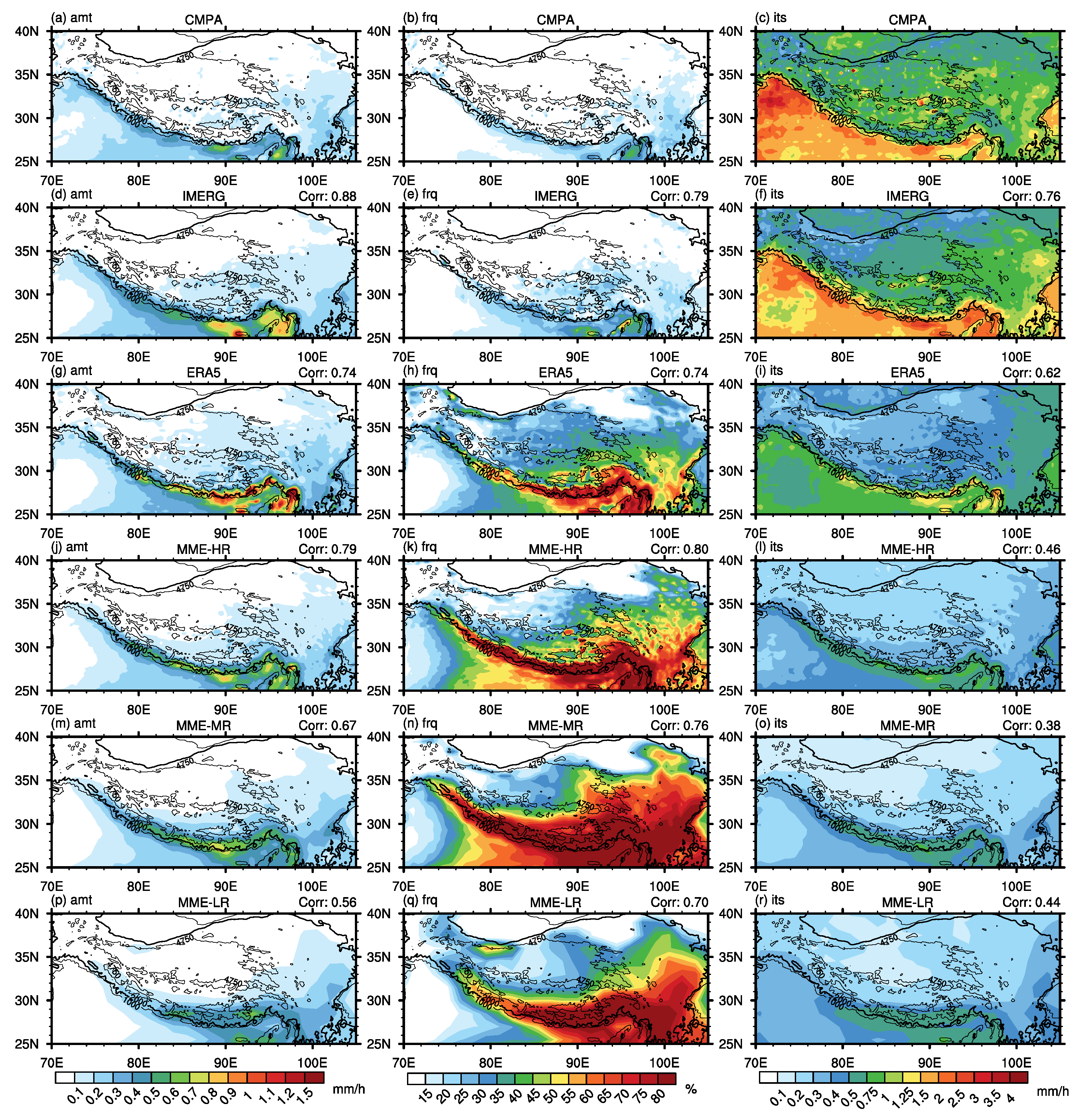
The spatial distribution of the JJA precipitation is shown in Figure 1; the time period for the CMPA was 2008–2014 and for the other datasets was 2000–2014. All the datasets showed a large precipitation amount along the Himalayas, diminishing toward the northwest TP (Figure 1 left column). Figure 1 demonstrates that the frequency distribution of the five datasets presented a decreasing trend similar to that of the precipitation amount. The region with the highest precipitation frequency was located in the south of the Himalayas and the eastern slope of the plateau. The right column in Figure 1 displays the distribution of the precipitation intensity. South Asia exhibited the highest intensity, while the central and eastern regions of the TP experienced greater intensity than the other parts of the plateau. We computed the spatial pattern correlation coefficients (CORRs) between the CMPA and other datasets. With the exception of the intensity, the CORRs between the MME-HR and the CMPA were higher than those between the ERA5 and CMPA. This suggests that the MME-HR, which has a comparable horizontal resolution to ERA5, can simulate the spatial characteristics of the precipitation amount and frequency more accurately. The CORRs between the MME-MR and the CMPA for the amount, frequency, and intensity were 0.67, 0.76, and 0.38, respectively, which were close to the CORRs between the MME-LR and the CMPA (0.56, 0.70, and 0.44). The MME-MR only had a slight improvement in simulating the distribution of the precipitation amount and frequency over the TP as compared to the MME-LR. Moreover, the increase in the resolution from the MME-LR to MME-HR showed little improvement in simulating the precipitation intensity.
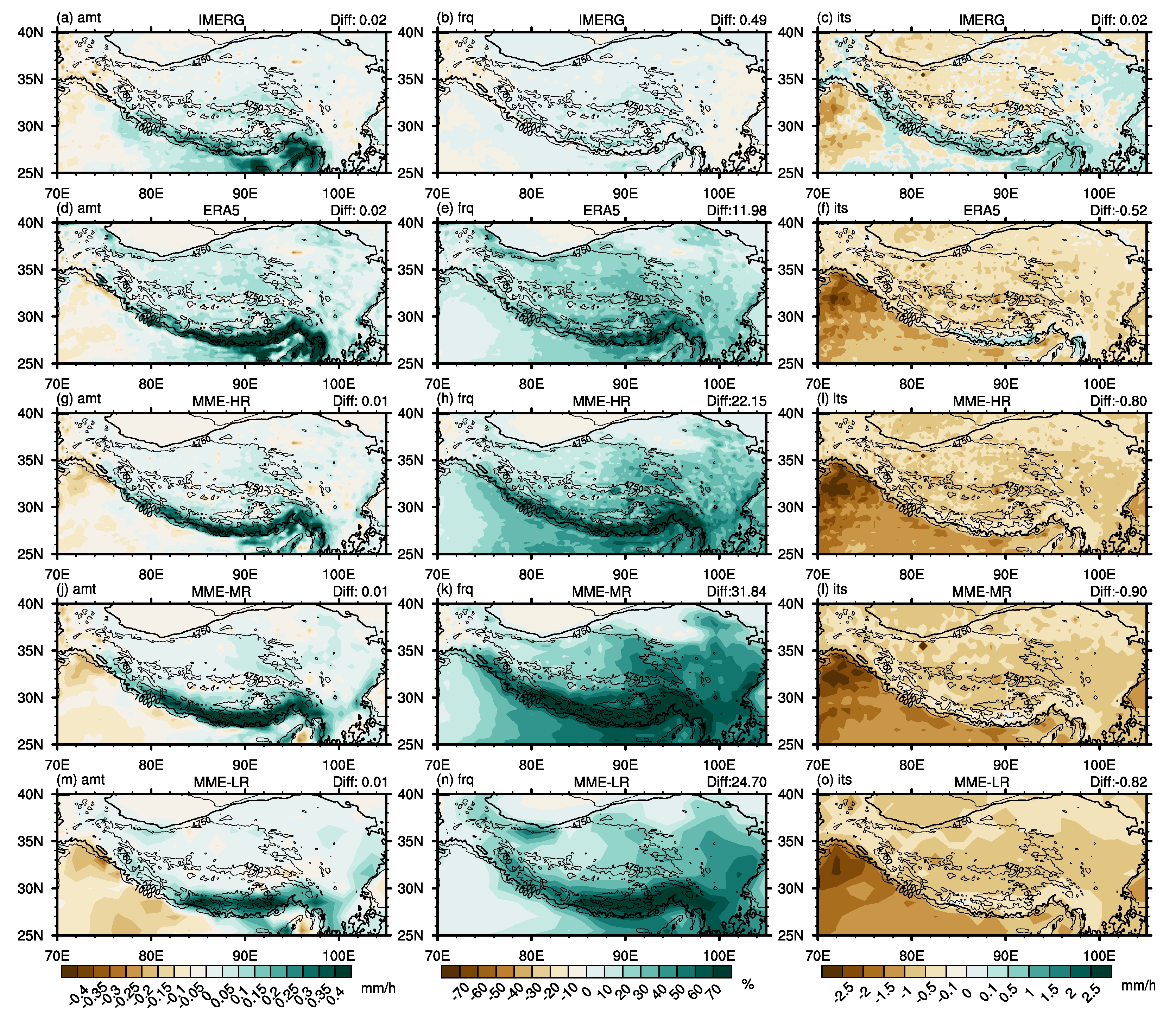
Although the spatial distribution characteristics of the precipitation amount and frequency in the three different resolutions of the MME were similar to those in CMPA, the MMEs obviously overestimated the amount (Figure 1g,j,m) and frequency (Figure 1h,k,n) over the Himalayas and the southeastern of TP. The three MMEs also underestimated the precipitation intensity over the entire study region (Figure 1i, l, o). Figure 2 shows the precipitation differences between the other five datasets and the CMPA. The simulation products, including the ERA5 and MMEs, all overestimated the precipitation amount in the TP, with the wettest region primarily situated in South Asia and the Himalayas (Figure 2d,g,j,m). The mean differences for the precipitation amount, frequency, and intensity between the CMPA and IMERG were 0.02 mm/h, 0.49%, and 0.02 mm/h, respectively. The ERA5 exhibited greater biases for both the frequency (11.98%) and the intensity (−0.52 mm/h) than the IMERG, and had a comparable precipitation amount bias of 0.02 mm/h (Figure 2d–f). Comparing the three distinct sets of MME, their spatial distribution characteristics of precipitation bias demonstrated a remarkable resemblance. In regions with complex topography, such as the Himalayas and the eastern edge of the TP, the overestimation of the precipitation was particularly severe (Figure 2g,j,m). In addition, all three MMEs overestimated the rainfall amount in the central TP. The wet biases in amount were primarily due to the overestimation of the precipitation frequency (Figure 2h,k,n), whereas the precipitation intensity was consistently underestimated across the study region, especially in the central part of the TP and the south of the Himalayas (Figure 2i,l,o). Nevertheless, the mean value of the precipitation bias within the study area did not decrease with the increase in the resolution. The MME-MR usually demonstrated the largest precipitation bias.
In order to evaluate the precipitation of the regions on the plateau with high altitude, the grids located at elevations over 2000 m were categorized as the grids on the main body of the TP. We contrasted the precipitation of these grids derived from the IMERG, ERA5, and MMEs with the value obtained from the CMPA as a reference. Table 2 presents the corresponding equation and optimal values of the three indexes used here, including the MB, RMSE, and CORR. We use the term “bias” in this paper to refer to the difference between the IMERG and the CMPA for the sake of conciseness. However, it is important to note that this difference is not truly a bias.
At grids located above 2000 m, the precipitation from the IMERG and CMPA were still relatively consistent. Compared to the entire study region, the IMERG exhibited a larger MB in the precipitation amount (0.03 mm/h) and frequency (2.87%) of the grids whose altitude was no less than 2000 m. These results show that the IMERG could still accurately depict the precipitation characteristics on the majority of the plateau, but the results of the satellite data in high-altitude areas were inferior to those in the low-altitude areas. Over the majority of the TP, the ERA5 demonstrated a higher bias in the precipitation amount and frequency (0.09 mm/h and 23.76%) compared to that of the entire study region, indicating that the ERA5 had relatively poor precipitation simulation capabilities for high-altitude regions. Likewise, the three sets of MME exhibited greater precipitation amount and frequency biases in the region at an altitude over 2000 m. However, the negative precipitation intensity bias of the three MMEs above 2000 m was smaller than the whole study region. The bolded font in Table 3 represents the statistical indices (MB, RMSE, and CORR) that were closest to the perfect values among the three MMEs. The MME-HR performed the best in the three different statistical indices of precipitation amount, frequency, and intensity. In descending order of the MME’s resolution, the MBs of the precipitation amount were 0.04, 0.07, and 0.06 mm/h, the frequency MBs were 26.70%, 39.13%, and 34.10%, and the intensity MBs were −0.51, −0.55, and −0.53 mm/h, respectively. The MMEs that exhibited the smallest RMSE values were consistent with the MBs. This is because, for the grids above an elevation of 2000 m, there was almost a uniform spatial pattern of precipitation bias, which showed a positive bias in the precipitation amount and frequency and a negative bias in the precipitation intensity, as demonstrated in Figure 2. Over the main body of the TP, the CORRs between the CMPA and MMEs were lower than those in the study region. These results, along with Figure 1 and Figure 2, indicate that the IMERG showed similar spatial characteristics of the precipitation to the CMPA; the MME-HR outperformed in the three sets of HighResMIP models with different resolutions; and increasing the model resolution had little impact on the simulation effects of the precipitation intensity.
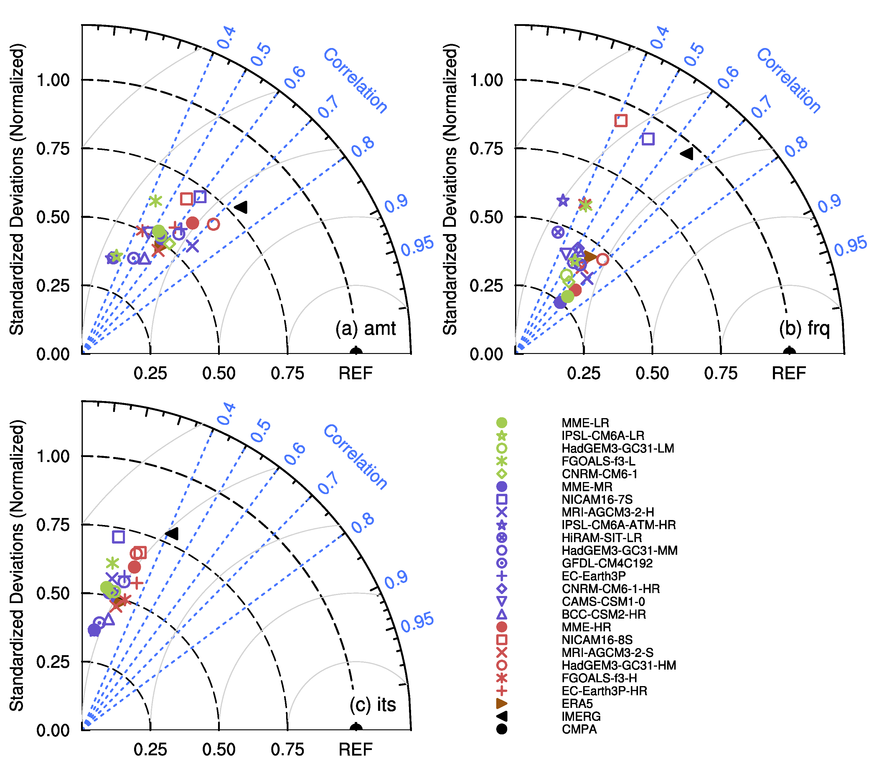
To illustrate each model’s ability to simulate the precipitation distribution over the Tibetan Plateau (TP), Taylor diagrams (Figure 3) were employed for a more intuitive and concise depiction. In Figure 3, the CMPA precipitation was used as the reference (labeled as REF). The colored markers represent models of different resolution categories, where red represents the HR models, yellow represents the MR models, and green represents the LR models. The color-filled circles represent the MMEs for the corresponding resolution ranges. The black-filled circle and the left-pointing and right-pointing triangles represent the precipitation of the CMPA, IMERG, and ERA5, respectively. Compared with the CMPA, the spatial correlation of almost all the GCMs (except the IPSL-CM6A-ATM-HR and HiRAM-SIT-LR) ranged from 0.4 to 0.75 for the precipitation amount and frequency (Figure 3a,b). The IPSL-CM6A-ATM-HR scored the lowest correlation ( for amount and for frequency), and the MRI-AGCM3-2-H scored the highest correlation for amount () and for frequency (). The normalized standard deviations from all the models were lower than 1.0, suggesting that the models exhibited smaller precipitation amount and frequency spatial variability than the CMPA. Only the NICAM16-7S and NICAM16-8S exhibited a precipitation amount and frequency spatial variability that closely matched the CMPA. The MME-HR and six models, comprising one HR model (HadGEM3-GC31-HM), four MR models (EC-Earth-3P, HadGEM3-GC31-MM, MRI-AGCM3-2-H, and NICAM16-7S), and one LR model (CNRM-CM6-1), outperformed the ERA5 in terms of the CORR and the normalized standard deviation when compared to the precipitation amount of the CMPA (Figure 3a). Only one model (HadGEM3-GC31-HM) outperformed the ERA5 in terms of both the CORR and standard deviation of the precipitation frequency (Figure 3b). The CORRs of all the models and the MMEs for the precipitation intensity (Figure 3c) were less than 0.4, which were much lower than that for the precipitation amount and frequency. Among the three sets of MMEs (the three solid colored circles), it was observed that the CORRS and standard deviations of the three different sets of MMEs exhibited varying degrees of consistency with the CMPA. Specifically, the MME-HR demonstrated a higher consistency with the CMPA, while the MME-MR and MME-LR exhibited similar but weaker consistency. The performance of the MME did not necessarily improve as the resolution increased. This is likely due to the fact that the MME-MR comprised more models than the MME-HR and MME-LR, and some models performed poorly among the precipitation amount, frequency, and intensity, such as the IPSL-CM6A-ATM-HR, HiRAM-SIT-LR, and the GFDL-CM4C192.
The diurnal cycle is used to examine the systematic timing and duration of precipitation events and as a means to improve model performance [45]. Chen et al. [9] analyzed 28 routine observation stations and found that the precipitation diurnal phase over the southeastern TP was closely related to the location of the station. Combining their findings with previous research, which solely used satellite data, it is necessary to use both station and satellite precipitation data when studying the diurnal variations in the precipitation in complex terrain areas. The CMPA, consisting of satellite data and gauge observations, is suitable for evaluation. When analyzing the phase of the diurnal cycle, the Fourier transformation is commonly used [46,47]. The 3-hourly precipitation time series was transformed into a composite daily cycle (comprising the average precipitation of eight time intervals) and then subjected to Fourier analysis. By analyzing the precipitation data from 100 stations located on the plateau, Li [10] discovered that 87% of the stations presented a significant single diurnal peak. Single-peak diurnal features were more prominent in grids that exhibited a higher first (diurnal) harmonic variance. Consistent with the criteria in Chen et al. [48], grids exhibiting a diurnal harmonic variance of no less than 60% were classified as single-peak grids.
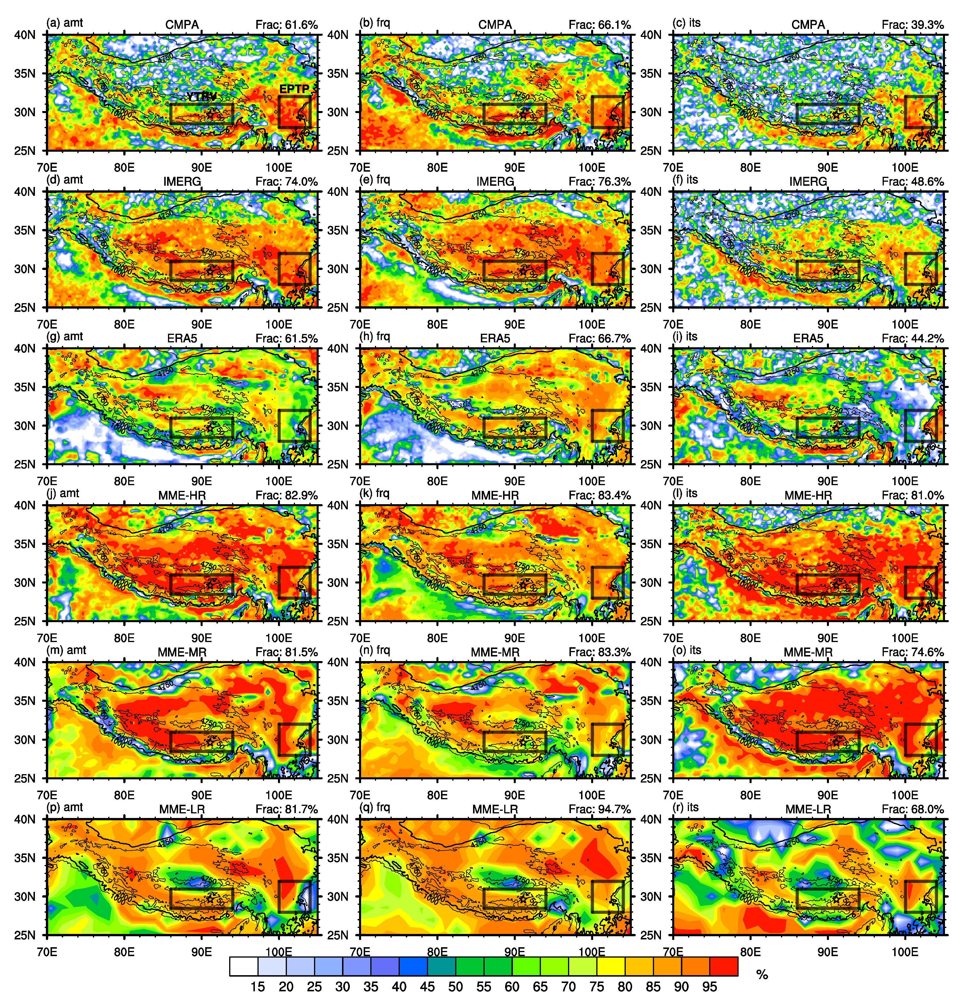
For the CMPA’s precipitation, 61.6% and 66.1% of grids exhibited single-peak characteristics in terms of the diurnal variance in the amount and frequency (Figure 4a,b). These grids were mainly located over the Himalayan ridge, South Asia, the Yarlung Tsangpo river valley (YTRV), and the eastern periphery of the TP (EPTP) regions. As shown in Figure 4d,e, about three-quarters of the grids in the spatial distribution of IMERG’s diurnal variance were single-peak grids, representing 74.0% for the amount and 76.3% for the frequency. The rainfall amount and frequency of the IMERG also exhibited clear single-peak diurnal phase characteristics in the three subregions mentioned above, presenting larger diurnal harmonic variance and wider area extent. The majority of the TP, except the north and west of the TP, showed single-peak characteristics. The proportion of single-peak grids for the precipitation amount (61.5%) and frequency (66.7%) in the ERA5 was comparable to that of the CMPA. However, the single-peak grid spatial pattern of the ERA5’s rainfall amount and frequency (Figure 4g,h) differed from the CMPA, mainly in terms of showing low (high) diurnal variance in the Himalayan ridge, South Asia, the YTRV, and the EPTP (the north and west of the TP) where the diurnal variance was high (low) in the CMPA. Compared with the CMPA, the precipitation amount and frequency derived from the three sets of MME all displayed a significantly stronger single-peak feature over the TP (Figure 4j,k,m,n,p,q). The MME-LR had a large proportion of single-peak grids among the three MMEs, 81.8% for the amount and 94.7% for the frequency, but had a lower value of first harmonic variance than the MME-HR and MME-MR. Nonetheless, the MME-HR (MME-LR) was not able to identify the single-peak feature of the frequency (amount) in regions with an altitude of less than 1000 m. Across the TP, all six datasets showed less prominent single-peak features in precipitation intensity compared to the amount and frequency, particularly in the CMPA, IMERG, and ERA5. In the CMPA, the single-peak grids of rainfall intensity occupied 39.3% of the TP, whereas in the MME-HR, they occupied 81.0%, over twice as much as in the CMPA.
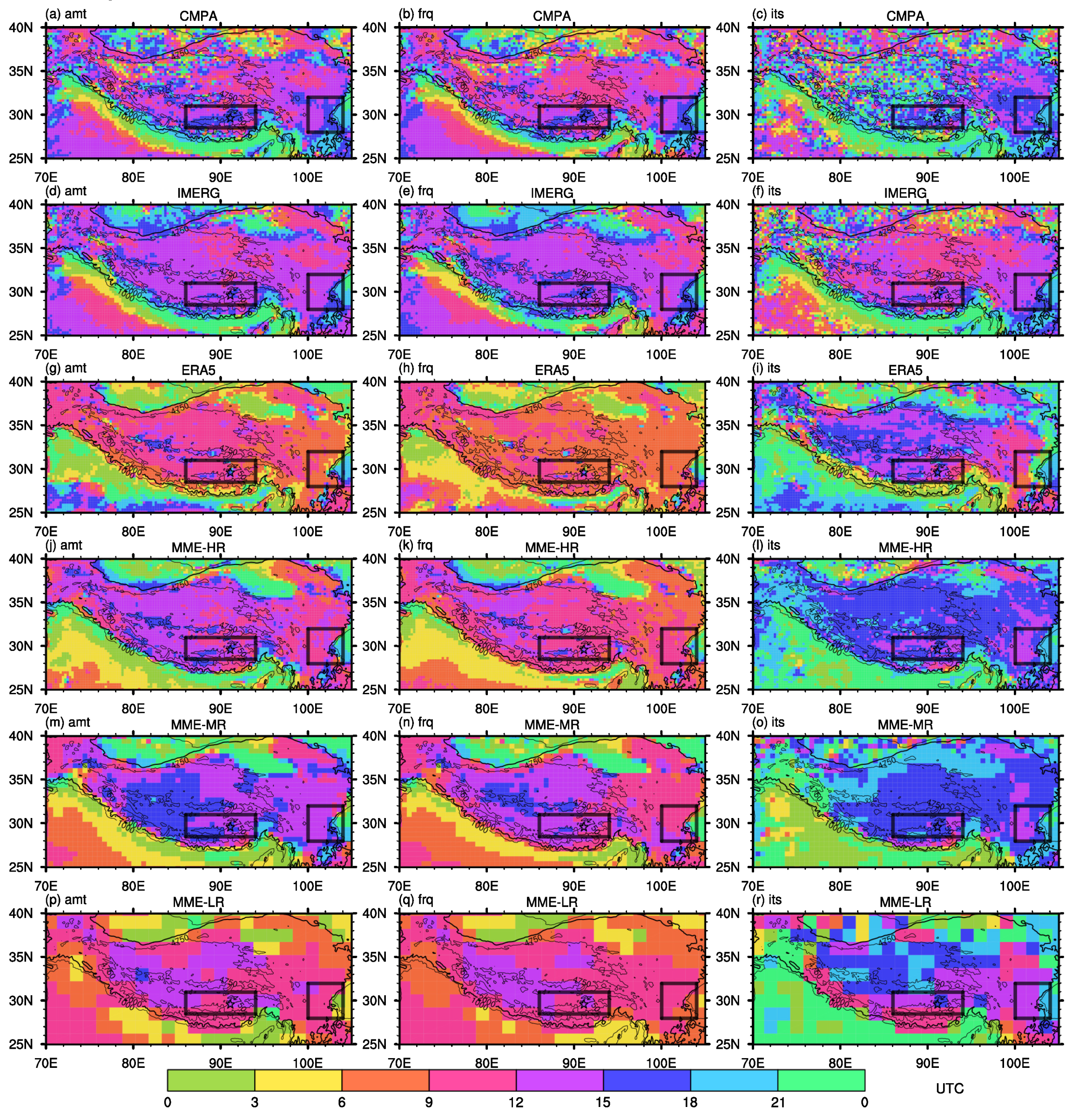
In the observational datasets, CMPA and IMERG, both the YTRV and EPTP exhibited a single-peak feature. In these two subregions, the ERA5 and MMEs also exhibited a notable single-peak feature and a significant overestimation of the precipitation. In addition, the YTRV and EPTP encompassed two distinctive topographic scales on the plateau. The YTRV is relatively narrow with a north–south width of tens of kilometers, and climate models with coarse resolution are unable to depict the north–south topography of the valley, while the EPTP has steep terrain, its horizontal scale can reach several hundred kilometers, and even climate models with coarse resolution can depict the slope in the region. Thus, we focused on analyzing the spatial distribution characteristics of the diurnal cycle in these two subregions. The two black rectangles in Figure 4 show the coverage of the YTRV and EPTP. Figure 5 displays the spatial distribution of the diurnal harmonic phase. It is noteworthy that the time interval of all datasets was processed into three hours, and the local time (LT) was approximately 5–7 h ahead of Coordinated Universal Time (UTC). For the CMPA and IMERG, most grids on the TP exhibited a diurnal phase of precipitation variables that occurred between the late afternoon to midnight (represented by the magenta and purple hues in Figure 5a–c,d–f, respectively). The ERA5’s precipitation amount and frequency (Figure 5g,h) tended to peak during midday to afternoon (orange and pink hues, respectively, 6–12 UTC). The three MMEs of the HighResMIP presented different diurnal features. Similar to the CMPA, the MME-HR’s precipitation amount and frequency diurnal peak (Figure 5j,k) revealed a late afternoon to a midnight peak (9–15 UTC) over the TP and midnight to early morning peak (18–0 UTC) in the Sichuan Basin. The MME-MR (Figure 5m,n) also displayed a pattern close to the CMPA but with more nighttime peaks (dark blue, 15–18 UTC) over the TP. With more afternoon peaks (9–12 UTC) and fewer late afternoon peaks (12–15 UTC) over the TP, the MME-LR’s spatial distribution of the precipitation amount and frequency diurnal peak (Figure 5p,q) resembled that of the ERA5. In the CMPA (Figure 5c), most grids over the TP reached the maximum precipitation intensity between midnight and early morning (15–21 UTC). The MME-HR and MME-MR (Figure 5l,o) were able to simulate this characteristic well, with a greater proportion of midnight peaks, while the ERA5 and MME-LR (Figure 5i,r) were unable to simulate this characteristic and instead generated more afternoon peaks.
By zooming in on the two subregions, more intricate details can be observed. The rainfall frequency diurnal phase and amount in the CMPA exhibited dependence on the elevation level in the YTRV (Figure 5a,b). The CMPA’s rainfall amount and frequency mostly peaked at evening and midnight (15–21 UTC) in the valley, while the amount and frequency peaked more frequently in the late afternoon (12–15 UTC) on the mountains. The diurnal phases of the IMERG, ERA5, MME-HR, and MME-MR (Figure 5d,e,g,h,j,k,m,n) likewise showed the nighttime peak in the bottom of the valley and an earlier peak in places with higher elevations. Nonetheless, compared to the CMPA, these datasets had lower nocturnal peak proportions. With coarser horizontal resolution, the MME-LR failed to reproduce the distribution features of the diurnal peak in the YTRV (Figure 5p,q). The MME-LR showed consistent afternoon to evening peaks within the region. From the eastern part to the western part of the EPTP (Figure 5a,b), the observational datasets’ (CMPA and IMERG) diurnal phase of the precipitation amount and frequency showed an intriguing colored pattern (purple–dark blue–light blue–green), representing the phase time transition from late afternoon (12–15 UTC) to midnight (15–21 UTC) and finally to early morning (21–0 UTC). The ERA5, MME-HR, and MME-MR reproduced the west-to-east variation of the precipitation amount’s diurnal phase in the EPTP (Figure 5g,j,m). Nevertheless, the spatial distribution characteristic of the MME-MR was more consistent with that of the CMPA, whereas the MME-HR (ERA5) simulated excessive afternoon (midday) peaks in the region above 2000 m. Despite the larger horizontal scale of the topography in the EPTP, the MME-LR struggled to replicate the spatial differences in the diurnal phase of the precipitation amount (Figure 5p). In the YTRV and EPTP, the diurnal phase of rainfall frequency resembled that of the rainfall amount but with a more pronounced afternoon peak (Figure 5h,k,n,q).
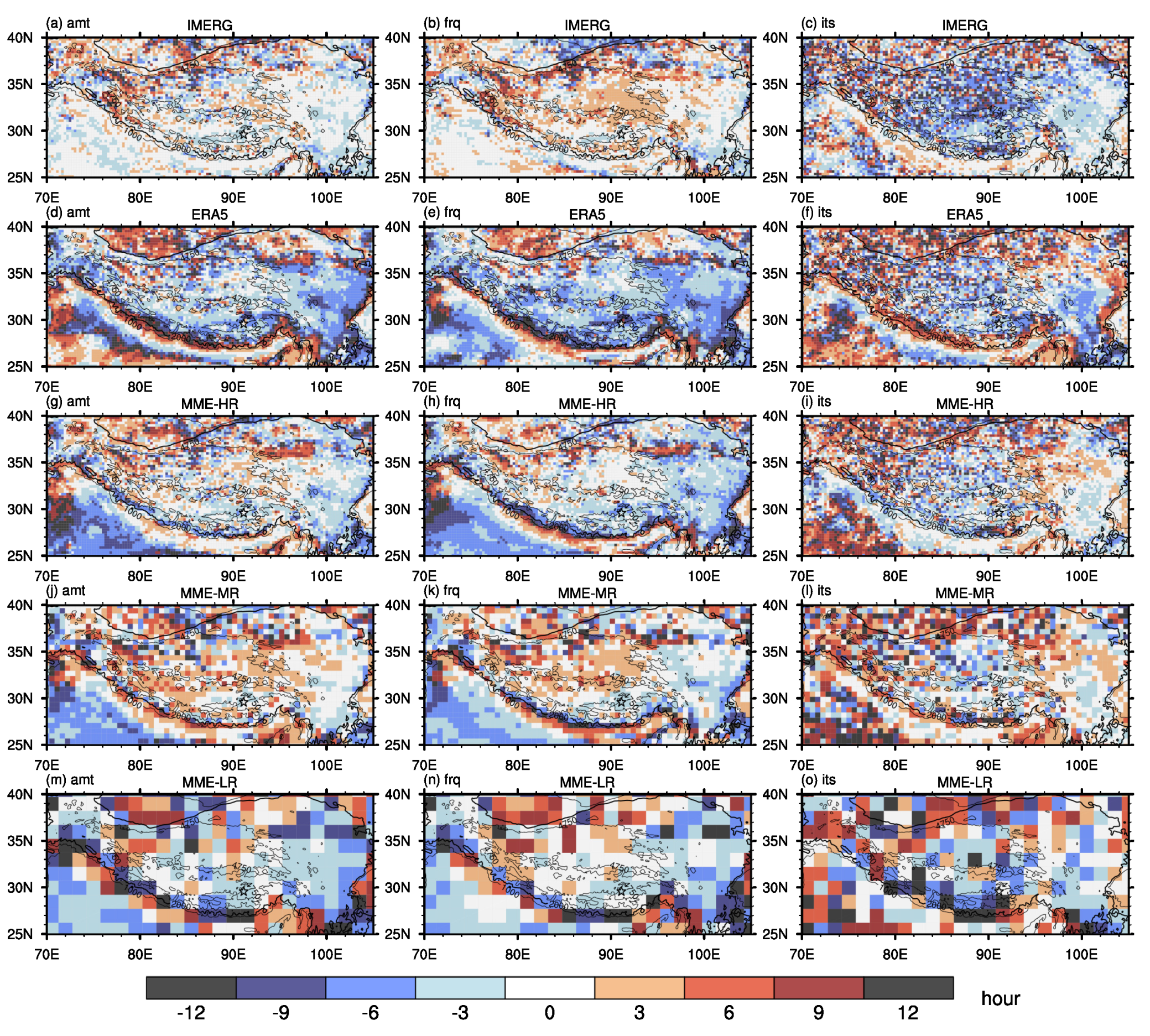
Over the TP, Figure 5 indicates that the ERA5, MME-HR, and MME-LR’s precipitation diurnal phases occurred earlier than the CMPA’s. The spatial distribution of the diurnal phase’s difference between each dataset with the CMPA is shown in Figure 6, allowing for further investigation of the characteristics of the deviation of the diurnal phase. Since all precipitation data were processed with the same temporal resolution as the HighResMIP (three-hourly), the difference between the diurnal phases is a multiple of three. The blue (red) shading in the figure indicates that the diurnal phase is either earlier (later) than that of the CMPA. The more hours advanced or delayed, the darker the color tone. The portion with a difference of more than nine hours is filled with a dark gray color. Figure 6a depicts that the diurnal phase of the IMERG precipitation amount was comparable to that of the CMPA, with an average diurnal phase difference of −0.1 h within the study area. Except for regions with low precipitation and weak single-peak features in the northwestern and northern portions of the TP, the bias between the IMERG and CMPA in the diurnal peak phase of rainfall amount was within three hours. On the central plateau, the diurnal phase of IMERG’s precipitation frequency (intensity) slightly lagged behind (leads) that of the CMPA (Figure 6b,c). For the ERA5 precipitation, 66.1% (74.2%) of grids over the TP exhibited earlier precipitation amount (frequency) diurnal phases than the CMPA (Figure 6d,e). The average diurnal phase difference of the ERA5 precipitation frequency within the study area was h, significantly larger than the three sets of HighResMIP MME. The MME-HR revealed a small difference in the diurnal phase of the precipitation amount on the main plateau, with an average deviation time of only h; the region with the greatest deviation was primarily South Asia (Figure 6g). In contrast to the other datasets, the diurnal phase of the rainfall amount in MME-MR occurred approximately 0.4 h later than the CMPA (Figure 6j).
Along the eastern and southern periphery of the TP, the diurnal phase differences of the ERA5 and the three MMEs’ precipitation frequency all showed a dark gray band. As the terrain altitude varies considerably in these regions, the diurnal phase of the CMPA and IMERG’s precipitation frequency swiftly transitioned from a nocturnal peak in the high-altitude regions to a morning peak in the low-altitude regions. In contrast, in the ERA5 and HighResMIP datasets, the diurnal peak time abruptly shifted from the afternoon in the high-altitude regions to the morning in the low-altitude regions. Among the three precipitation characteristics, the intensity exhibited the fewest single-peak features. As a result, the ERA5 and three MMEs’ distribution of the diurnal phase differences was more disorderly (Figure 6f,i,l,o). In the following section, based on the terrain altitude of grid points, a more comprehensive analysis of the precipitation diurnal variation for HighResMIP MME with different resolutions over the plateau is presented.
3.2. Elevation Dependence of Precipitation Characteristics
In addition to other topographical factors, altitude has a significant impact on the climatic spatial distribution of precipitation [49,50]. The results of model simulations of the relationship between precipitation and altitude can also reflect the models’ capacity to simulate precipitation.
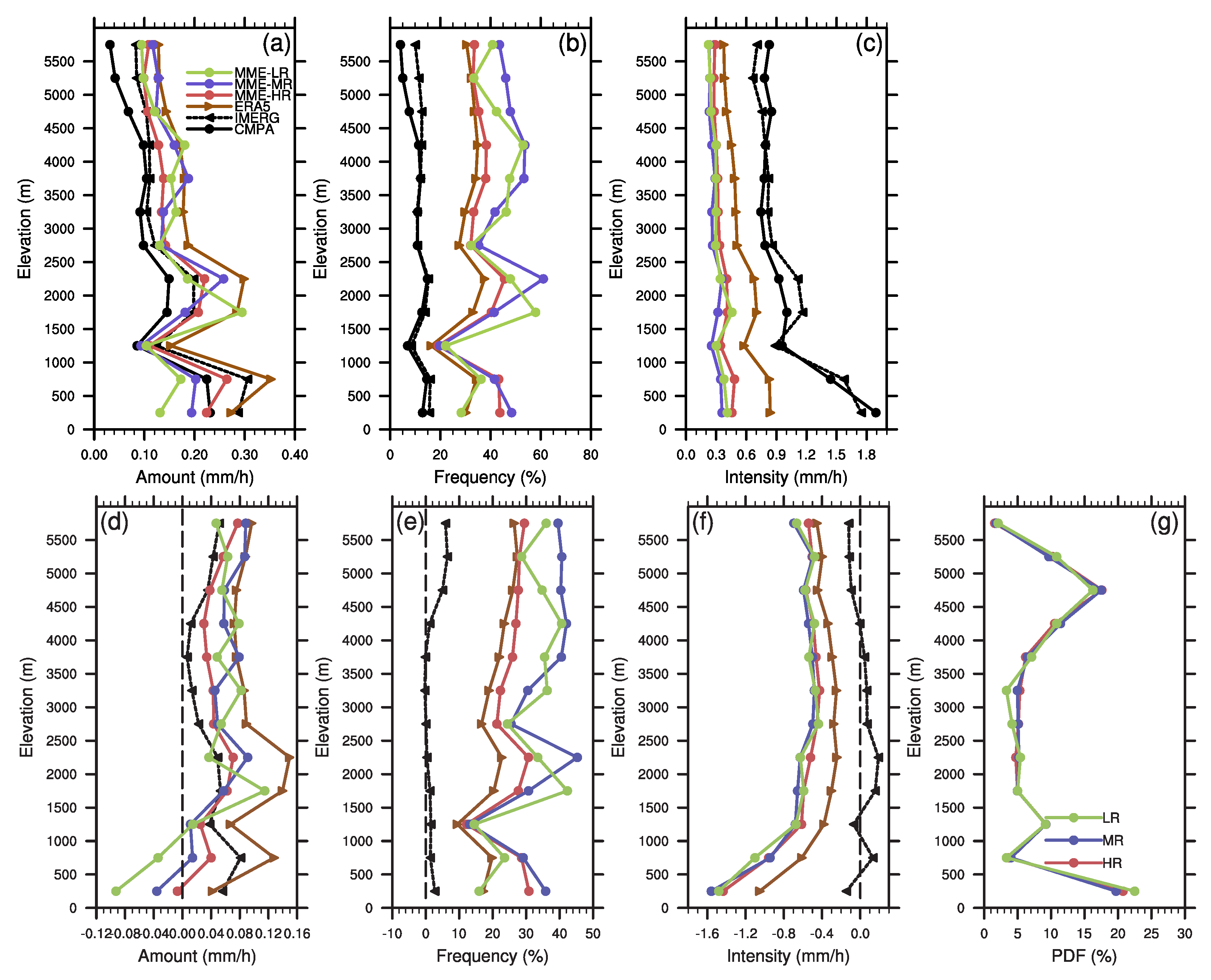
Some studies evaluating high-resolution models have started to consider the elevation dependence of precipitation [48,51]. The elevation dependence of precipitation variables over the TP are illustrated in Figure 7a–c. Except for the altitude range between 1000 and 1500 m, the precipitation amount decreased with increasing altitude according to both the CMPA (black solid line) and IMERG (black dashed line) rainfall (Figure 7a). The elevation dependence of the precipitation frequency derived from the CMPA and IMERG were nonlinear below 4000 m, and the CMPA’s precipitation frequency decreased with the increasing altitude above 4000 m, whereas IMERG’s precipitation frequency remained constant (Figure 7b). The CMPA and IMERG’s precipitation intensity also decreased with increasing elevation, and the average precipitation intensity of the grids whose elevation was less than 1000 m was substantially greater than that of grids whose elevation was greater than 1000 m (Figure 7c). The ERA5 (brown line) and the three MMEs (red, violet, and green lines) reproduced the trend of the decreasing precipitation amount with the altitude but significantly overestimated the precipitation above 1500 m in altitude. Figure 7d demonstrates that the ERA5 had the largest positive bias in the precipitation amount across almost all altitude ranges, while the MME-HR had the smallest positive bias. The ERA5 had a smaller positive frequency bias and a smaller negative intensity bias than the three MMEs (Figure 7e,f). The MME-HR had the smallest bias for precipitation frequency at various altitudes among different resolutions of the HighResMIP MME, while the MMEs at different resolutions had nearly identical simulation biases for precipitation intensity at varying altitudes. Therefore, the positive precipitation bias of the MME-HR was less than that of the MME-MR and LR at each altitude range.
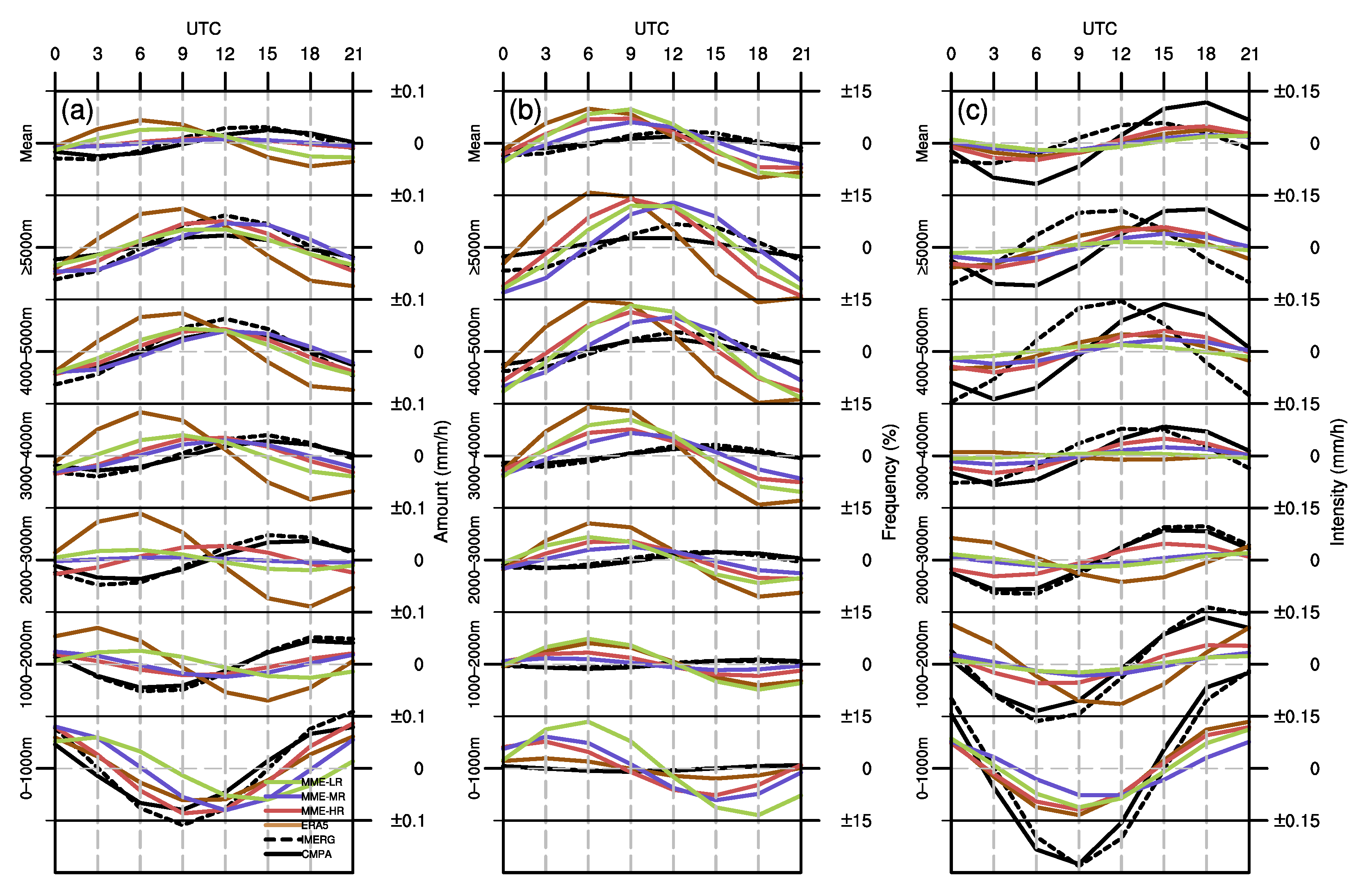
Figure 5 demonstrates that the distribution characteristics of the precipitation diurnal phase over the TP varied with the terrain elevation for all the precipitation datasets. The diurnal harmonic curves at various altitudes are shown in Figure 8 to study in further detail how the diurnal phase of the precipitation varied with the altitude. The horizontal black solid lines in the figure demarcate various altitude ranges, while the gray dashed lines in the center of each block represent the zero lines. In the top panel, the diurnal cycle of the region mean is shown, and the other panels correspond to a range of elevations. In areas with low elevation, the diurnal amplitude of the observational datasets’ precipitation amount (Figure 8a, black solid and dashed lines) was larger, and the diurnal peak time occurred primarily at 21 UTC (approximately 2–4 LT). As the altitude increased, the diurnal amplitude of the precipitation amount decreased, and the diurnal peak progressively advanced to 12 UTC. (17–19 LT). The brown line in Figure 8a shows that the ERA5 did not accurately replicate the variation in the precipitation amount’s diurnal harmonic curve with altitude, with the exception of the curve below 1000 m, which was consistent with the CMPA. In the altitude range between 1000 and 4000 m, the ERA5 even exhibited anti-phase characteristics compared to the observational precipitation. Contrary to the observation, the diurnal peak time of the ERA5 precipitation amount was delayed with the increasing altitude, from 3 UTC (8–10 LT) in the 1000–2000 m altitude range to 9 UTC (14–16 LT) above 5000 m. The diurnal harmonic curves of the precipitation amount for the three HighResMIP MMEs (Figure 8a, red, violet, and green line) were more consistent with the CMPA in the altitude range below 1000 m and above 3000 m, while their simulation performance between 1000 and 3000 m was less satisfactory. The bias in the amount and frequency of the three MMEs also sharply increased between 1000 and 3000 m (Figure 7d,e). Most grids with an elevation between 1000 and 3000 m were situated on the slope. These grids had larger topographic relief, and their subgrid terrain was more complex than other regions of the plateau. The model’s poor performance in simulating precipitation in the slopes was reflected not only by the wet bias in the precipitation but also by the deviation in the diurnal variation.
In addition, the ERA5 and MMEs had trouble replicating the elevation dependence of the diurnal variation in the precipitation frequency and intensity. With the increase in the altitude, the CMPA and IMERG’s diurnal amplitude of precipitation frequency increased, while their diurnal amplitude of precipitation intensity decreased and then increased. In the ERA5 and MMEs, the diurnal amplitude of the frequency showed an increasing trend with the altitude and overestimated the amplitude at all altitude ranges compared to the observations (Figure 8b). Both the ERA5 and MMEs’ diurnal amplitude of intensity reached a maximum at the 0–1000 m altitude range and underestimated the amplitude at various altitudes. At elevations greater than 1000 m, the diurnal variation amplitude of the precipitation intensity in the ERA5 decreased with the altitude, whereas the three sets of the MME remained unchanged.
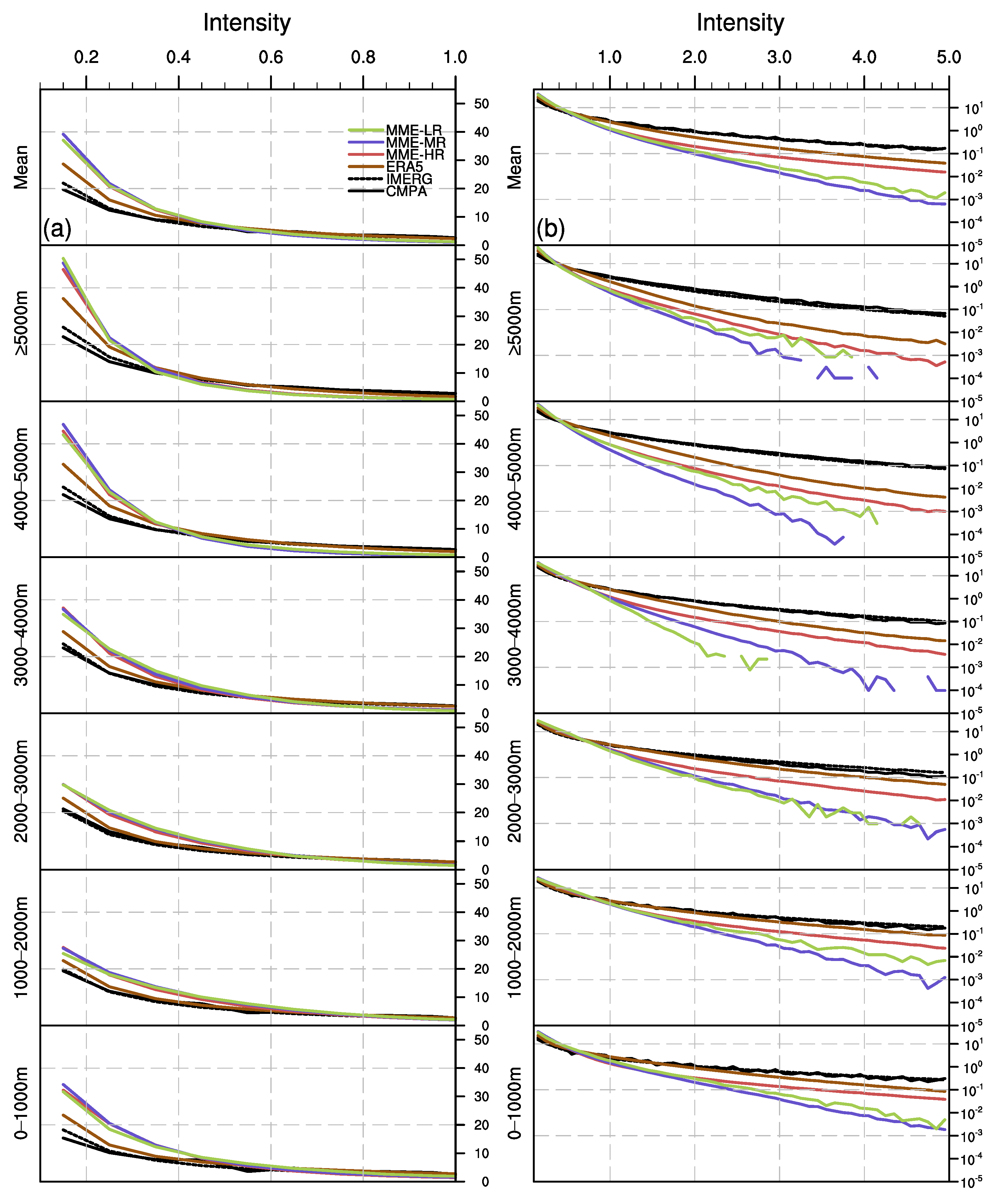
The precipitation frequency–intensity structure is an essential aspect of climatological rainfall characteristics and plays a crucial role in evaluating model performance [52]. It displays the occurrence frequency of the precipitation with varying intensities. Figure 9 depicts the frequency–intensity structure curves of various precipitation data at different altitudes. The left column presents the precipitation frequency for weak intensities (0.1–1 mm/h), while the right column shows the frequency for all intensities with logarithmic coordinates. Most climate models exhibit a bias in the frequency–intensity structure of precipitation, overestimating the light precipitation while underestimating the heavy precipitation [52,53,54]. The ERA5 and the three sets of HighResMIP MME also tended to overestimate the frequency of the light precipitation and underestimate that of the heavy precipitation. In addition, as the altitude increased, the underestimation of the frequency of the heavy precipitation became more severe. Despite the ERA5 performing poorly in simulating the variation of the diurnal cycle with the altitude, its simulation of the frequency–intensity structure of the precipitation at various altitudes was substantially superior to that of the HighResMIP. In particular, the frequency of light precipitation occurring below 4000 m and heavy precipitation occurring below 3000 m was more consistent with the observation. The simulation effect of the MME-HR on the frequency–intensity structure was second only to that of the ERA5. At the heavy precipitation end, the MME-HR simulated more occurrence frequency and a larger maximum intensity, while the MME-LR (MME-MR) rarely produced precipitation with an intensity over 4 mm/h at an altitude above 2000 m (3000 m). In terms of light precipitation, there was little distinction between the three, and all substantially overestimated the frequency of the weak precipitation’s occurrence. Moreover, the bias in both the ERA5 and the HighResMIP MMEs regarding the precipitation frequency–intensity structure was amplified with higher altitudes.
4. Discussion
From the evaluation of the spatial distribution of the precipitation in Section 3.1, both the ERA5 and HighResMIP MMEs showed small precipitation amount biases over the TP. However, this does not necessarily indicate that the simulation of precipitation in the plateau area was reasonable. The small bias in the precipitation amount was due to the fact that the overestimation of the precipitation frequency and the underestimation of the precipitation intensity cancelled each other out. Further analysis of the precipitation frequency–intensity structure revealed that the overestimation of the frequency of light precipitation and the underestimation of the frequency of heavy precipitation jointly contributed to the simulation bias in both the frequency and intensity. The different intensities of precipitation in the GCMs may correspond to different physical processes. For instance, heavy precipitation might be mainly produced by convective parameterization schemes that release locally unstable energy. In order to comprehend the essence of model precipitation bias, it is necessary to conduct more in-depth analyses.
The primary objective of the HighResMIP is to determine the robust benefits of the increased horizontal model resolution based on the multimodel ensemble simulations [26]. The multimodel ensemble approach is widely used but still has some deficiencies. It may be difficult to ignore model performance altogether, and it is hard to make optimal use of the information available. Therefore, it is necessary to directly evaluate the simulation effect of each model during the model evaluation process. Moreover, the number of models significantly impacts the results of the MME. In this paper, there were only five and four models in the high-resolution and low-resolution categories, respectively. Several institutions have submitted results using multiple horizontal resolutions of the same model, including EC-Earth3P and EC-Earth3P-HR, HadGEM3-GC31-HM, HadGEM3-GC31-MM, and HadGEM3-GC31-LM, etc. To verify the reliability of the conclusions of the article, we evaluated a new multimodel ensemble mean comprised of models from the same institution with high resolution (EC-Earth3P-HR, HadGEM3-GC31-HM, MRI-AGCM3-2-S, and NICAM16-8S) and with middle resolution (EC-Earth3P, HadGEM3-GC31-MM, MRI-AGCM3-2-H, and NICAM16-7S). The obtained conclusions were similar to the article’s main conclusions; that is, the precipitation simulation effect of the high-resolution group was superior to that of the middle-resolution group (figures not shown). However, Xin et al. [27] compared five HighResMIP models (BCC-CSM2-HR, CNRM-CM6-1-HR, EC-Earth3P-HR, HadGEM3-GC31-HH, and MPI-ESM1-2-XR) and their lower resolution models (BCC-CSM2-MR, CNRM-CM6-1, EC-Earth3P, HadGEM3-GC31-MM, and MPI-ESM1-2-HR) and found that, over the TP, most high-resolution models exhibited inferior performance compared to their lower resolution versions. The study period and model chosen will affect the MME evaluation results, and we must also recognize the limitations of the MME method and use it more carefully.
It is noteworthy that this study only considered elevation when evaluating the model’s ability to reproduce the relationship between precipitation and topography. However, the precipitation distribution is influenced by other topographic factors as well, including orographic slope and orientation [55]. Real precipitation distributions are a combination of elevation and slope, in addition to other factors. Therefore, the sign of the overall feedback will depend on the geometry and orientation of the mountain range and the local climate regime. It would be intriguing to investigate the specific effects of windward/leeward slopes and the blocking effect, which can significantly impact the flow of air through the mountains. Consequently, there are some uncertainties in the evaluation, which must be resolved through a comprehensive analysis of additional topographic factors.
5. Conclusions
This study evaluated the performance of the CMIP6 HighResMIP climate models and the ERA5 in simulating summer precipitation over the Tibetan Plateau. The HighResMIP models were classified into three categories based on their horizontal resolution to assess the impact of the model resolution on the simulation of precipitation in complex terrain areas.
The major results can be summarized as follows:
- The horizontal resolution of the HighResMIP MME-HR is comparable to that of the ERA5, and both show a comparable ability in simulating the precipitation in the TP. The precipitation amount and frequency derived from the MME-HR are slightly better than that of the ERA5, indicated by a higher spatial correlation and a closer standard deviation with the CMPA. The MME-HR overestimates the occurrence of single-peak grids in the majority of the TP but still manages to simulate the spatial distribution of the single-peak grids and diurnal phase better than the ERA5. Despite its diurnal peak occurring earlier than the CMPA, the difference between the MME-HR and the CMPA’s diurnal peak is smaller than that between the ERA5 and CMPA. In terms of the elevation dependence of the precipitation, the MME-HR shows a smaller deviation in the precipitation amount at various altitudes compared to the CMPA. The ERA5 incorrectly simulates the relationship between the diurnal phase and altitude. In the CMPA and IMERG, the diurnal phase of precipitation amount advances with the increasing elevation from early morning to evening, whereas in the ERA5, it delays from early morning to afternoon. However, the ERA5 can better simulate the precipitation frequency–intensity structure at different altitudes.
- The simulation effect of CMIP6 HighResMIP’s precipitation in the TP does not necessarily improve with the increase in the model’s horizontal resolution, even though the MME-HR shows the best simulation effects among the three MMEs. On the one hand, increasing the resolution enhances the HighResMIP model’s ability to simulate the diurnal variation in precipitation. With the increase in horizontal resolution, the issue of the earlier diurnal peak in the HighResMIP models at highlands is alleviated, and the elevation dependence of the precipitation’s diurnal variation is better characterized. On the other hand, the improvement in the resolution has little impact on the simulation effect of precipitation intensity, but a lower model resolution restricts the generation of heavy precipitation in high-altitude areas.
- The ERA5 and different resolutions of the HighResMIP MMEs share common precipitation biases in the TP. All of them overestimate the precipitation amount and frequency while underestimating the intensity. Secondly, they cannot accurately simulate the diurnal variations in the precipitation in the elevated area. In addition, they have the issue of overestimating the frequency of the weak precipitation and underestimating that of the heavy precipitation. These biases are related to the altitude: the interval with the greatest diurnal phase bias is in the altitude range of 1000–3000 m, which is mostly located in the periphery of the TP with a large topographic relief; the deviation in the precipitation frequency–intensity structure increases with increasing altitude.
This study provides important insights into the spatial distribution and altitude dependence of precipitation characteristics in satellite-gauge merged product, HighResMIP models, and reanalysis data over the TP. Thus, the results can help us in comprehending the global climate models’ precipitation bias in complex terrain.
Author Contributions
Conceptualization, T.C.; methodology, T.C.; software, Y.Z.; validation, T.C. and N.L.; formal analysis, T.C.; investigation, T.C.; resources, Y.Z.; data curation, T.C. and N.L.; writing—original draft preparation, T.C.; writing—review and editing, Y.Z. and N.L.; visualization, T.C.; supervision, Y.Z.; project administration, Y.Z.; funding acquisition, Y.Z. All authors have read and agreed to the published version of the manuscript.
Funding
This research was funded by the National Natural Science Foundation of China, Grant No. 42225505, No.U2142204, No.42005039, and the S&T Development Fund of Chinese Academy of Meteorological Sciences, No. 2022KJ007.
Institutional Review Board Statement
Not applicable.
Informed Consent Statement
Not applicable.
Data Availability Statement
The CMIP6 HighResMIP, IMERG, ERA5, and GTOPO30 datasets are publicly available. CMIP6 HighResMIP can be found here: https://esgf-node.llnl.gov/search/cmip6/ (accessed on 12 April 2022). IMERG can be found here: https://pmm.nasa.gov/data-access/downloads/gpm (accessed on 1 June 2022). ERA5 can be found here: https://cds.climate.copernicus.eu/cdsapp#!/dataset/reanalysis-era5-single-levels?tab=overview/ (accessed on 1 June 2022). GTOPO30 can be found here: https://www.usgs.gov/centers/eros/science/usgs-eros-archive-digital-elevation-global-30-arc-second-elevation-gtopo30 (accessed on 28 Janurary 2021).
Conflicts of Interest
The authors declare no conflict of interest.
References
- Qiu, J. China: The third pole. Nature 2008, 454, 393–397. [Google Scholar] [CrossRef] [Green Version]
- Ye, D.; Gao, Y. Meteorology of the Qinghai-Xizang (Tibet) Plateau; Science Press: Beijing, China, 1979. (In Chinese) [Google Scholar]
- Anders, A.M.; Roe, G.H.; Hallet, B.; Montgomery, D.R.; Finnegan, N.J.; Putkonen, J. Spatial patterns of precipitation and topography in the Himalaya. Spec. Pap.-Geol. Soc. Am. 2006, 398, 39–53. [Google Scholar]
- Kuo, H.L.; Qian, Y. Influence of the Tibetian Plateau on cumulative and diurnal changes of weather and climate in summer. Mon. Weather Rev. 1981, 109, 2337–2356. [Google Scholar] [CrossRef]
- Fujinami, H.; Nomura, S.; Yasunari, T. Characteristics of diurnal variations in convection and precipitation over the southern Tibetan Plateau during summer. Sola 2005, 1, 49–52. [Google Scholar] [CrossRef] [Green Version]
- Ueno, K.; Fujii, H.; Yamada, H.; Liu, L. Weak and frequent monsoon precipitation over the Tibetan Plateau. J. Meteorol. Soc. Jpn. Ser. II 2001, 79, 419–434. [Google Scholar] [CrossRef] [Green Version]
- Yu, R.; Zhou, T.; Xiong, A.; Zhu, Y.; Li, J. Diurnal variations of summer precipitation over contiguous China. Geophys. Res. Lett. 2007, 34, 223–234. [Google Scholar] [CrossRef] [Green Version]
- Liu, X.; Bai, A.; Liu, C. Diurnal variations of summertime precipitation over the Tibetan Plateau in relation to orographically-induced regional circulations. Environ. Res. Lett. 2009, 4, 045203. [Google Scholar] [CrossRef]
- Chen, H.; Yuan, W.; Li, J.; Yu, R. A possible cause for different diurnal variations of warm season rainfall as shown in station observations and TRMM 3B42 data over the southeastern Tibetan Plateau. Adv. Atmos. Sci. 2012, 29, 193–200. [Google Scholar] [CrossRef]
- Li, J. Hourly station-based precipitation characteristics over the Tibetan Plateau. Int. J. Climatol. 2018, 38, 1560–1570. [Google Scholar] [CrossRef]
- Chen, Q.; Ge, F.; Jin, Z.; Lin, Z. How well do the CMIP6 HighResMIP models simulate precipitation over the Tibetan Plateau? Atmos. Res. 2022, 279, 106393. [Google Scholar] [CrossRef]
- Reinman, S.L. Intergovernmental panel on climate change (IPCC). Ref. Rev. 2012, 26, 41–42. [Google Scholar] [CrossRef]
- Meehl, G.A.; Boer, G.J.; Covey, C.; Latif, M.; Stouffer, R.J. The coupled model intercomparison project (CMIP). Bull. Am. Meteorol. Soc. 2000, 81, 313–318. [Google Scholar] [CrossRef]
- Eyring, V.; Bony, S.; Meehl, G.A.; Senior, C.A.; Stevens, B.; Stouffer, R.J.; Taylor, K.E. Overview of the Coupled Model Intercomparison Project Phase 6 (CMIP6) experimental design and organization. Geosci. Model Dev. 2016, 9, 1937–1958. [Google Scholar] [CrossRef] [Green Version]
- Xin, X.; Wu, T.; Zhang, J.; Yao, J.; Fang, Y. Comparison of CMIP6 and CMIP5 simulations of precipitation in China and the East Asian summer monsoon. Int. J. Climatol. 2020, 40, 6423–6440. [Google Scholar] [CrossRef] [Green Version]
- Gusain, A.; Ghosh, S.; Karmakar, S. Added value of CMIP6 over CMIP5 models in simulating Indian summer monsoon rainfall. Atmos. Res. 2020, 232, 104680. [Google Scholar] [CrossRef]
- Ayugi, B.; Zhihong, J.; Zhu, H.; Ngoma, H.; Babaousmail, H.; Rizwan, K.; Dike, V. Comparison of CMIP6 and CMIP5 models in simulating mean and extreme precipitation over East Africa. Int. J. Climatol. 2021, 41, 6474–6496. [Google Scholar] [CrossRef]
- Luo, N.; Guo, Y.; Chou, J.; Gao, Z. Added value of CMIP6 models over CMIP5 models in simulating the climatological precipitation extremes in China. Int. J. Climatol. 2022, 42, 1148–1164. [Google Scholar] [CrossRef]
- Lee, Y.C.; Wang, Y.C. Evaluating Diurnal Rainfall Signal Performance from CMIP5 to CMIP6. J. Clim. 2021, 34, 7607–7623. [Google Scholar] [CrossRef]
- Gulizia, C.; Camilloni, I. Comparative analysis of the ability of a set of CMIP3 and CMIP5 global climate models to represent precipitation in South America. Int. J. Climatol. 2015, 35, 583–595. [Google Scholar] [CrossRef]
- Su, F.; Duan, X.; Chen, D.; Hao, Z.; Cuo, L. Evaluation of the global climate models in the CMIP5 over the Tibetan Plateau. J. Clim. 2013, 26, 3187–3208. [Google Scholar] [CrossRef] [Green Version]
- Chen, L.; Frauenfeld, O.W. A comprehensive evaluation of precipitation simulations over China based on CMIP5 multimodel ensemble projections. J. Geophys. Res. Atmos. 2014, 119, 5767–5786. [Google Scholar] [CrossRef]
- Zhu, H.; Jiang, Z.; Li, J.; Li, W.; Sun, C.; Li, L. Does CMIP6 inspire more confidence in simulating climate extremes over China? Adv. Atmos. Sci. 2020, 37, 1119–1132. [Google Scholar] [CrossRef]
- Zhang, Y.; Li, J. Impact of moisture divergence on systematic errors in precipitation around the Tibetan Plateau in a general circulation model. Clim. Dyn. 2016, 47, 2923–2934. [Google Scholar] [CrossRef] [Green Version]
- Kim, H.J.; Wang, B.; Ding, Q. The global monsoon variability simulated by CMIP3 coupled climate models. J. Clim. 2008, 21, 5271–5294. [Google Scholar] [CrossRef]
- Haarsma, R.J.; Roberts, M.J.; Vidale, P.L.; Senior, C.A.; Bellucci, A.; Bao, Q.; Chang, P.; Corti, S.; Fučkar, N.S.; Guemas, V.; et al. High resolution model intercomparison project (HighResMIP v1. 0) for CMIP6. Geosci. Model Dev. 2016, 9, 4185–4208. [Google Scholar] [CrossRef] [Green Version]
- Xin, X.; Wu, T.; Jie, W.; Zhang, J. Impact of higher resolution on precipitation over China in CMIP6 HighResMIP models. Atmosphere 2021, 12, 762. [Google Scholar] [CrossRef]
- Haarsma, R.; Acosta, M.; Bakhshi, R.; Bretonnière, P.A.; Caron, L.P.; Castrillo, M.; Corti, S.; Davini, P.; Exarchou, E.; Fabiano, F.; et al. HighResMIP versions of EC-Earth: EC-Earth3P and EC-Earth3P-HR–description, model computational performance and basic validation. Geosci. Model Dev. 2020, 13, 3507–3527. [Google Scholar] [CrossRef]
- Bao, Q.; Liu, Y.; Wu, G.; He, B.; Li, J.; Wang, L.; Wu, X.; Chen, K.; Wang, X.; Yang, J.; et al. CAS FGOALS-f3-H and CAS FGOALS-f3-L outputs for the high-resolution model intercomparison project simulation of CMIP6. Atmos. Ocean. Sci. Lett. 2020, 13, 576–581. [Google Scholar] [CrossRef]
- Roberts, M.J.; Baker, A.J.; Blockley, E.W.; Calvert, D.; Coward, A.C.; Hewitt, H.T.; Jackson, L.C.; Kuhlbrodt, T.; Mathiot, P.; Roberts, C.D.; et al. Description of the resolution hierarchy of the global coupled HadGEM3-GC3.1 model as used in CMIP6 HighResMIP experiments. Geosci. Model Dev. 2019, 12, 4999–5028. [Google Scholar] [CrossRef] [Green Version]
- Mizuta, R.; Yoshimura, H.; Murakami, H.; Matsueda, M.; Endo, H.; Ose, T.; Kamiguchi, K.; Hosaka, M.; Sugi, M.; Yukimoto, S.; et al. Climate Simulations Using MRI-AGCM3.2 with 20-km Grid. J. Meteorol. Soc. Jpn. 2012, 90, 233–258. [Google Scholar] [CrossRef] [Green Version]
- Kodama, C.; Ohno, T.; Seiki, T.; Yashiro, H.; Noda, A.T.; Nakano, M.; Yamada, Y.; Roh, W.; Satoh, M.; Nitta, T.; et al. The Nonhydrostatic ICosahedral Atmospheric Model for CMIP6 HighResMIP simulations (NICAM16-S): Experimental design, model description, and impacts of model updates. Geosci. Model Dev. 2021, 14, 795–820. [Google Scholar] [CrossRef]
- Wu, T.; Lu, Y.; Fang, Y.; Xin, X.; Li, L.Z.X.; Li, W.; Jie, W.; Zhang, J.; Liu, Y.; Zhang, L.; et al. The Beijing Climate Center Climate System Model (BCC-CSM): The main progress from CMIP5 to CMIP6. Geosci. Model Dev. 2019, 12, 1573–1600. [Google Scholar] [CrossRef] [Green Version]
- Rong, X.; Li, J.; Chen, H.; Su, J.; Hua, L.; Zhang, Z.; Xin, Y. The CMIP6 Historical Simulation Datasets Produced by the Climate System Model CAMS-CSM. Adv. Atmos. Sci. 2020, 38, 285–295. [Google Scholar] [CrossRef]
- Voldoire, A.; Saint-Martin, D.; Sénési, S.; Decharme, B.; Alias, A.; Chevallier, M.; Colin, J.; Guérémy, J.; Michou, M.; Moine, M.P.; et al. Evaluation of CMIP6 DECK Experiments With CNRM-CM6-1. J. Adv. Model. Earth Syst. 2019, 11, 2177–2213. [Google Scholar] [CrossRef] [Green Version]
- Zhao, M.; Golaz, J.C.; Held, I.; Guo, H.; Balaji, V.; Benson, R.; Chen, J.H.; Chen, X.; Donner, L.; Dunne, J.; et al. The GFDL global atmosphere and land model AM4. 0/LM4. 0: 2. Model description, sensitivity studies, and tuning strategies. J. Adv. Model. Earth Syst. 2018, 10, 735–769. [Google Scholar] [CrossRef] [Green Version]
- Harris, L.M.; Lin, S.; Tu, C.Y. High-Resolution Climate Simulations Using GFDL HiRAM with a Stretched Global Grid. J. Clim. 2016, 29, 4293–4314. [Google Scholar] [CrossRef]
- Boucher, O.; Servonnat, J.; Albright, A.L.; Aumont, O.; Balkanski, Y.; Bastrikov, V.; Bekki, S.; Bonnet, R.; Bony, S.; Bopp, L.; et al. Presentation and Evaluation of the IPSL-CM6A-LR Climate Model. J. Adv. Model. Earth Syst. 2020, 12, e2019MS002010. [Google Scholar] [CrossRef]
- He, B.; Bao, Q.; Wang, X.; Zhou, L.; Wu, X.; Liu, Y.; Wu, G.; Chen, K.; He, S.; Hu, W.; et al. CAS FGOALS-f3-L Model Datasets for CMIP6 Historical Atmospheric Model Intercomparison Project Simulation. Adv. Atmos. Sci. 2019, 36, 771–778. [Google Scholar] [CrossRef] [Green Version]
- Shen, Y.; Zhao, P.; Pan, Y.; Yu, J. A high spatiotemporal gauge-satellite merged precipitation analysis over China. J. Geophys. Res. Atmos. 2014, 119, 3063–3075. [Google Scholar] [CrossRef]
- Joyce, R.J.; Janowiak, J.E.; Arkin, P.A.; Xie, P. CMORPH: A method that produces global precipitation estimates from passive microwave and infrared data at high spatial and temporal resolution. J. Hydrometeorol. 2004, 5, 487–503. [Google Scholar] [CrossRef]
- Hou, A.Y.; Skofronick-Jackson, G.; Kummerow, C.D.; Shepherd, J.M. Global precipitation measurement. In Precipitation: Advances in Measurement, Estimation and Prediction; Springer: Berlin/Heidelberg, Germany, 2008; pp. 131–169. [Google Scholar]
- Hou, A.Y.; Kakar, R.K.; Neeck, S.; Azarbarzin, A.A.; Kummerow, C.D.; Kojima, M.; Oki, R.; Nakamura, K.; Iguchi, T. The global precipitation measurement mission. Bull. Am. Meteorol. Soc. 2014, 95, 701–722. [Google Scholar] [CrossRef]
- Hersbach, H.; Bell, B.; Berrisford, P.; Hirahara, S.; Horányi, A.; Muñoz-Sabater, J.; Nicolas, J.; Peubey, C.; Radu, R.; Schepers, D.; et al. The ERA5 global reanalysis. Q. J. R. Meteorol. Soc. 2020, 146, 1999–2049. [Google Scholar] [CrossRef]
- Trenberth, K.E.; Dai, A.; Rasmussen, R.M.; Parsons, D.B. The changing character of precipitation. Bull. Am. Meteorol. Soc. 2003, 84, 1205–1218. [Google Scholar] [CrossRef]
- McGarry, M.M.; Reed, R.J. Diurnal variations in convective activity and precipitation during phases II and III of GATE. Mon. Weather Rev. 1978, 106, 101–113. [Google Scholar] [CrossRef]
- Oki, T.; Musiake, K. Seasonal change of the diurnal cycle of precipitation over Japan and Malaysia. J. Appl. Meteorol. Climatol. 1994, 33, 1445–1463. [Google Scholar] [CrossRef]
- Chen, T.; Li, J.; Zhang, Y.; Chen, H.; Li, P.; Che, H. Evaluation of Hourly Precipitation Characteristics from a Global Reanalysis and Variable-Resolution Global Model over the Tibetan Plateau by Using a Satellite-Gauge Merged Rainfall Product. Remote Sens. 2023, 15, 1013. [Google Scholar] [CrossRef]
- Basist, A.; Bell, G.D.; Meentemeyer, V. Statistical relationships between topography and precipitation patterns. J. Clim. 1994, 7, 1305–1315. [Google Scholar] [CrossRef]
- Yuan, W.; Xu, H.; Yu, R.; Li, J.; Zhang, Y.; He, N. Regimes of rainfall preceding regional rainfall events over the plain of Beijing City. Int. J. Climatol. 2018, 38, 4979–4989. [Google Scholar] [CrossRef] [Green Version]
- Zhou, X.; Yang, K.; Ouyang, L.; Wang, Y.; Jiang, Y.; Li, X.; Chen, D.; Prein, A. Added value of kilometer-scale modeling over the third pole region: A CORDEX-CPTP pilot study. Clim. Dyn. 2021, 57, 1673–1687. [Google Scholar] [CrossRef]
- Li, J.; Yu, R.; Yuan, W.; Chen, H.; Sun, W.; Zhang, Y. Precipitation over East Asia simulated by NCAR CAM5 at different horizontal resolutions. J. Adv. Model. Earth Syst. 2015, 7, 774–790. [Google Scholar] [CrossRef]
- Chen, M.; Dickinson, R.E.; Zeng, X.; Hahmann, A.N. Comparison of precipitation observed over the continental United States to that simulated by a climate model. J. Clim. 1996, 9, 2233–2249. [Google Scholar] [CrossRef]
- Dai, A.; Trenberth, K.E. The diurnal cycle and its depiction in the Community Climate System Model. J. Clim. 2004, 17, 930–951. [Google Scholar] [CrossRef]
- Roe, G.H.; Montgomery, D.R.; Hallet, B. Orographic precipitation and the relief of mountain ranges. J. Geophys. Res. Solid Earth 2003, 108. [Google Scholar] [CrossRef]
Figure 1.
The spatial distribution of the precipitation, including the amount (mm/h, left column), frequency (%, middle column), and intensity (mm/h, right column), derived from the CMPA (a–c), IMERG (d–f), ERA5 (g–i), MME-HR (j–l), MME-MR (m–o), and MME-LR (p–r). The number in the upper-right of each subplot is the spatial correlation coefficient between the CMPA and the other five datasets. The thin black contours represent elevations of 1000 and 4750 m, and the thick black contour indicates the terrain at an elevation of 2000 m.

Figure 2.
The spatial distribution of the precipitation difference, including the amount (mm/h, left column), frequency (%, middle column), and intensity (mm/h, right column), between the IMERG (a–c), ERA5 (d–f), MME-HR (g–i), MME-MR (j–l), and the MME-LR (m–o) and the CMPA. The number in the upper-right of each subplot is the area mean differences. The thin black contours represent elevations of 1000 and 4750 m, and the thick black contour indicates the terrain at an elevation of 2000 m.

Figure 3.
Taylor diagrams of the precipitation (a) amount, (b) frequency, and (c) intensity at the grids’ elevation over 2000 m.
Figure 3.
Taylor diagrams of the precipitation (a) amount, (b) frequency, and (c) intensity at the grids’ elevation over 2000 m.

Figure 4.
The spatial distribution of the diurnal harmonic’s variance (%), including the amount (left column), frequency (middle column), and intensity (right column), derived from the CMPA (a–c), IMERG (d–f), ERA5 (g–i), MME-HR (j–l), MME-MR (m–o), and MME-LR (p–r). The number in the upper-right of each subplot is the percentage of single-peak grids. The two black rectangles represent subregions exhibiting significant single-peak diurnal features (YTRV: Yarlung Tsangpo River Valley, and EPTP: Eastern Periphery of the Tibetan Plateau). The thin black contours represent elevations of 1000 and 4750 m, and the thick black contour indicates the terrain at an elevation of 2000 m.

Figure 5.
The spatial distribution of the diurnal harmonic’s phase (UTC), including the amount (left column), frequency (middle column), and intensity (right column), derived from the CMPA (a–c), IMERG (d–f), ERA5 (g–i), MME-HR (j–l), MME-MR (m–o), and MME-LR (p–r). The two black rectangles represent the subregions exhibiting significant single-peak diurnal features (YTRV and EPTP). The thin black contours represent elevations of 1000 and 4750 m, and the thick black contour indicates the terrain at an elevation of 2000 m.

Figure 6.
The spatial distribution of the precipitation diurnal phase differences (h), including the amount (left column), frequency (middle column), and intensity (right column), between the IMERG (a–c), ERA5 (d–f), MME-HR (g–i), MME-MR (j–l), and MME-LR (m–o) and the CMPA. The thin black contours represent elevations of 1000 and 4750 m, and the thick black contour indicates the terrain at an elevation of 2000 m.

Figure 7.
Elevation dependence of the precipitation variables (a–c) and the differences between the other datasets and the CMPA (d–f) in the study area. The first column represents the precipitation amount (mm/h), the second column represents the frequency (%), and the third column represents the intensity (mm/h). The black solid line stands for the CMPA dataset, the black dashed line for the IMERG, the brown solid line for the ERA5, red for the MME-HR, violet for the MME-MR, and green for the MME-LR, or their differences with the CMPA. (g) The probability density function (PDF) of the grids’ altitude for different resolution groups.

Figure 8.
The elevation dependence of the precipitation diurnal harmonic, including the (a) amount (mm/h), (b) frequency (%), and (c) intensity (mm/h). Solid black horizontal lines are used to separate the altitude blocks, with a gray horizontal line at the center of each block marking the zero line. The top panel is the mean diurnal harmonic over the TP, and the other panels correspond to a range of elevations. The left Y-axis labels indicate the altitude intervals for each panel. The right Y-axis labels indicate the diurnal harmonic curve values. Positive (negative) values above (below) the zero line represent the values of the diurnal harmonic curve on the right Y-axis. The X-axis indicates the hour (UTC) of the diurnal cycle. The black solid (dashed) line stands in for the CMPA (IMERG) dataset, brown for the ERA5, red for the MME-HR, violet for the MME-MR, and green for the MME-LR.

Figure 9.
The elevation dependence of the precipitation frequency–intensity structure. (a) Frequency distribution with intensities smaller than 1 mm/h; (b) frequency distribution with all intensities using logarithmic coordinates. Solid black horizontal lines are used to separate the altitude blocks, with a gray horizontal line at the center of each block marking the zero line. The top panel is the mean diurnal harmonic over the TP, and the other panels correspond to a range of elevations. The left Y-axis labels indicate the altitude intervals for each panel. The right Y-axis labels indicate the diurnal harmonic curve values. The X-axis indicates various rainfall intensities (mm/h). The black solid (dashed) line stands in for the CMPA (IMERG) dataset, brown for the ERA5, red for the MME-HR, violet for the MME-MR, and green for the MME-LR.


Table 1.
Model names, modeling centers, and the atmospheric resolutions of 19 CMIP6-HighResMIP GCMS.
Table 1.
Model names, modeling centers, and the atmospheric resolutions of 19 CMIP6-HighResMIP GCMS.
| Label (Regridded Resolution) | Model | Institute | Resolution (Lat × Lon) |
|---|---|---|---|
| High Resolution 0.27 × 0.27) | EC-Earth3P-HR | EC-Earth Consortium, Europe [28] | 0.35 × 0.35 |
| FGOALS-f30H | Chinese Academy of Sciences [29] | 0.25 × 0.25 | |
| HadGEM3-GC31-HM | Met Office Hadley Centre, UK [30] | 0.23 × 0.23 | |
| MRI-AGCM3-2-S | Meteorological Research Institute, Japan [31] | 0.19 × 0.19 | |
| NICAM16-8S | JAMSTEC-AORI-R-CCS, Japan [32] | 0.28 × 0.28 | |
| Middle Resolution (0.56 × 0.56) | BCC-CSM2-HR | Beijing Climate Center, China [33] | 0.45 × 0.45 |
| CAMS-CSM1-0 | Chinese Academy of Meteorological Sciences, China [34] | 0.47 × 0.47 | |
| CNRM-CM6-1-HR | National Centre for Meteorological Research, France [35] | 0.50 × 0.50 | |
| EC-Earth3P | EC-Earth Consortium, Europe [28] | 0.70 × 0.70 | |
| GFDL-CM4C192 | NOAA, Geophysical Fluid Dynamics Laboratory, USA [36] | 0.50 × 0.63 | |
| HadGEM3-GC31-MM | Met Office Hadley Centre, UK [30] | 0.56 × 0.83 | |
| HiRAM-SIT-LR | Research Center for Environmental Changes, Taiwan [37] | 0.50 × 0.50 | |
| IPSL-CM6A-ATM-HR | L’Institut Pierre-Simon Laplace, France [38] | 0.50 × 0.70 | |
| MRI-AGCM3-2-H | Meteorological Research Institute, Japan [31] | 0.56 × 0.56 | |
| NICAM16-7S | JAMSTEC-AORI-R-CCS, Japan [32] | 0.56 × 0.56 | |
| Low Resolution (1.50 × 1.50) | CNRM-CM6-1 | National Centre for Meteorological Research, France [35] | 1.40 × 1.40 |
| FGOALS-f3-L | Chinese Academy of Sciences [39] | 1.00 × 1.25 | |
| HadGEM3-GC31-LM | Met Office Hadley Centre, UK [30] | 1.25 × 1.88 | |
| IPSL-CM6A-LR | Institut Pierre Simon Laplace, France [38] | 1.26 × 2.50 |
Table 2.
Equations and the optimal values of the statistical indices.
| Statistical Index | Equation | Optimal Value |
|---|---|---|
| MB (Mean Bias) | 0 | |
| RMSE (Root Mean Square Error) | 0 | |
| CORR (Spatial Correlation Coefficient) | 1 |
, the CMPA precipitation variables; , the CMPA mean precipitation variables; , the IMERG, ERA5, and MME precipitation estimates, respectively; , the IMERG, ERA5, and MME mean precipitation variables, respectively; n, the corresponding grids.
Table 3.
Precipitation statistical error indices from the IMERG, ERA5, and MMEs versus the CMPA for grids with elevations over 2000 m during JJA 2000–2014.
Table 3.
Precipitation statistical error indices from the IMERG, ERA5, and MMEs versus the CMPA for grids with elevations over 2000 m during JJA 2000–2014.
| Variables | Metrics | CMPA | IMERG | ERA5 | MME-HR | MME-MR | MME-LR |
|---|---|---|---|---|---|---|---|
| Amount (mm/h, except CORR) | Mean | 0.08 | 0.11 | 0.17 | 0.13 | 0.15 | 0.14 |
| MB | / | 0.03 | 0.09 | 0.04 | 0.07 | 0.06 | |
| RMSE | / | 0.07 | 0.15 | 0.10 | 0.13 | 0.13 | |
| CORR | / | 0.73 | 0.60 | 0.65 | 0.57 | 0.53 | |
| Frequency (%, except CORR) | Mean | 9.34 | 12.20 | 33.10 | 36.04 | 48.70 | 43.26 |
| MB | / | 2.87 | 23.76 | 26.70 | 39.13 | 34.10 | |
| RMSE | / | 6.74 | 27.01 | 32.33 | 46.19 | 39.72 | |
| CORR | / | 0.65 | 0.61 | 0.68 | 0.66 | 0.67 | |
| Intensity (mm/h, except CORR) | Mean | 0.81 | 0.79 | 0.45 | 0.30 | 0.26 | 0.28 |
| MB | / | −0.02 | −0.36 | −0.51 | −0.55 | −0.53 | |
| RMSE | / | 0.31 | 0.44 | 0.56 | 0.63 | 0.58 | |
| CORR | / | 0.41 | 0.29 | 0.31 | 0.20 | 0.17 |
The bolded font represents the statistical indices (MB, RMSE, and CORR) that are closest to the perfect values among the three MMEs.
Disclaimer/Publisher’s Note: The statements, opinions and data contained in all publications are solely those of the individual author(s) and contributor(s) and not of MDPI and/or the editor(s). MDPI and/or the editor(s) disclaim responsibility for any injury to people or property resulting from any ideas, methods, instructions or products referred to in the content. |
© 2023 by the authors. Licensee MDPI, Basel, Switzerland. This article is an open access article distributed under the terms and conditions of the Creative Commons Attribution (CC BY) license (https://creativecommons.org/licenses/by/4.0/).
Share and Cite
MDPI and ACS Style
Chen, T.; Zhang, Y.; Li, N. Evaluation of CMIP6 HighResMIP Models and ERA5 Reanalysis in Simulating Summer Precipitation over the Tibetan Plateau. Atmosphere 2023, 14, 1015. https://doi.org/10.3390/atmos14061015
AMA Style
Chen T, Zhang Y, Li N. Evaluation of CMIP6 HighResMIP Models and ERA5 Reanalysis in Simulating Summer Precipitation over the Tibetan Plateau. Atmosphere. 2023; 14(6):1015. https://doi.org/10.3390/atmos14061015
Chicago/Turabian StyleChen, Tianru, Yi Zhang, and Nina Li. 2023. "Evaluation of CMIP6 HighResMIP Models and ERA5 Reanalysis in Simulating Summer Precipitation over the Tibetan Plateau" Atmosphere 14, no. 6: 1015. https://doi.org/10.3390/atmos14061015
Note that from the first issue of 2016, this journal uses article numbers instead of page numbers. See further details here.