On the Mechanisms of a Snowstorm Associated with a Low-Level Cold Front and Low-Level Jet in the Western Mountainous Region of the Junggar Basin, Xinjiang, Northwest China

Abstract

Snowstorms frequently hit large parts of the Northern Hemisphere, and their causative factors have been drawing increasing attention in recent years. As the first in-depth study on the mechanisms of a snowstorm associated with a low-level cold front (LLCF) and low-level westerly jet (LLWJ) in the western mountainous region of the Junggar Basin, Xinjiang, based on both observations and numerical simulation, the major findings of this work are as follows: At the early stage, instabilities were mainly dominated by inertial instability (II) occurring near the core region of the LLWJ, while the lower level was mainly controlled by the baroclinic component of moist potential vorticity (MPV2), which was mainly contributed by the vertical shear of the horizontal wind, which is also located near the LLWJ. At the later stage, II was released significantly, whereas the MPV2 still supported snowfall clouds. Further analysis based on the decomposition of the frontogenetical forcing required for the release of the instabilities indicated that the slantwise term was the major contributor, whereas convergence and deformation also played significant roles at low levels above the windward slope. The slantwise term resulted from the combined effects of baroclinicity due to the LLCF and the inhomogeneity of the momentum due to the LLWJ.

1. Introduction

Snowstorms are one of the major catastrophic weather events in mid- and high latitudes in winter and often pose serious threats to lives, properties, transportation, agriculture, and energy supply via heavy snow, high wind, low temperature, and low visibility [1,2,3,4,5,6]. In recent years, snowstorms have frequently hit large parts of the Northern Hemispheric continents, and increasing attention has been shown to the causes of snowstorms [7]. Although numerical weather prediction has made great progress so far, accurate prediction of local heavy snowfall weather is still challenging for meteorologists [8]. Gaining a better understanding of the mechanisms controlling the occurrence and development of snowstorms is very important to improve snowstorm forecasts [9,10,11], and it has some implications for improving the seasonal runoff predictions and projections of the development and utilization of water resources [12,13,14].

The mechanisms underlying the occurrence and development of snowstorms are complicated. Many studies have analyzed the causes and mechanisms of snowstorms in a climatological context [7,15,16,17,18]. Wang et al. [18] investigated the results of snowstorms in northern China from 1961 to 2014 and showed that the snowstorms corresponded to the negative phases of the North Atlantic Oscillation (NAO) and the Arctic Oscillation (AO). Zhou et al. [7] stated that the shift from negative to positive polarity in the mid-1990s in the main pattern of snowstorms in northern China from 1961 to 2014 was linked to the southward shift of the polar frontal jet and the northward shift of the upper subtropical jet in the troposphere. Sun et al. [15] studied the first two leading modes of the interannual variability of the frequency of snowfall events (FSE) in China in the winter from 1986 to 2018. They found that the positive phase of the first leading mode (EOF1) is primarily characterized by positive FSE anomalies in northeastern to northwestern China, as well as negative FSE anomalies in the Three-River-Source region. On the contrary, the positive phase of the second leading mode (EOF2) is mainly characterized by positive FSE anomalies in central-eastern China.

Furthermore, there are many aspects within the context of land surface patterns and mesoscale weather systems that can play important roles in the mechanisms of snowstorms, such as oceans, lakes, complex terrain, cold fronts, and jet streams [19,20,21,22]. For example, Aikins et al. [23] studied the role of a cross-barrier jet and turbulence on an orographic snowfall and stated that the presence of cross-barrier jets favors the shear-induced turbulent zones, and this turbulence is a key mechanism in enhancing snow growth. Furthermore, Campbell et al. [9] studied the influences of orography and coastal geometry on a sea-effect snowstorm over Hokkaido Island, Japan. They found that the orographic flow deflection by the coastal mountains produced convergence and ascent along the elongated enhancement region near the entrance to Ishikari Bay. In addition, Ma et al. [24] studied the mechanisms of vertical velocity and vertical kinetic energy changes during heavy snowfall in complex terrains. They stated that the passage of a cold front increases the surface pressure due to the arrival of the cold high behind, resulting in changes in the vertical pressure gradient force and the dry air column buoyancy, which in turn resulted in the development of vertical motion. Gehring et al. [25] found that orographic gravity waves (GWs) induced over the ice ridge upstream of Davis in the Vestfold Hills, East Antarctica, were responsible for snowfall sublimation through a foehn effect, and there was almost no precipitation reaching the ground at Davis, despite a strong moisture advection that occurred during this event.

Moreover, the frontogenetical forcing and some accompanying instabilities have also been considered important mechanisms of snowstorms [26,27,28]. For example, Sanders and Bosart [29] investigated a heavy snowstorm event that affected major cities in the northeastern United States and stated that the snowfall is attributable mainly to frontogenetical forcing and symmetric instability (SI). Similarly, Wang and Ding [30] suggested that frontogenetical forcing played an important role in the occurrence of a strong snowstorm event in North China in 1986. Schultz and Schumacher [31] stated that the release of conditional symmetric instability (CSI) is predicated upon slantwise air parcel lifting beyond the condensation level to the level of free slantwise convection (LFSC). They also claimed that the frontogenetical circulation is one of the mechanisms that can produce an ascent flow required to lift an air parcel forcibly to its LFSC. Schumacher et al. [32] also stated that the major snowbands were associated with frontogenesis along a cold front, and the minor snowbands formed due to the release of CSI and II. Taylor et al. [33] investigated the synoptic/mesoscale dynamics responsible for an unusually heavy snowstorm in the southern US where the convective instability (CI) and CSI, terrain blocking, and a double low-level jet (LLJ) development process played an important, in addition to the synoptic scale process. Li et al. [34] investigated the mechanism of a terrain-influenced snowstorm event in Northeast China. Their numerical experiments showed that without the influence of the Changbai Mountains, the release of CI and II within a weak frontogenetical environment was responsible for the maintenance of the snowbands. They also stated that the release of the CI at the mid-level and other low-level or near-surface instabilities (II, CI, or CSI) contributed to the formation of the snowbands. In addition, some studies have been conducted to investigate the contribution of each sub-terms of the frontogenetical forcing to heavy precipitation by decomposing the frontogenesis function [35]. Xu et al. [36] analyzed the strong precipitation of the Meiyu front in the Zhejiang Province and found that the low-level frontal generation was mainly contributed by the convergence term and deformation term, and the slantwise term played a negative role. Furthermore, He et al. [37] found that the largest contribution to frontogenesis was the deformation term, whereas the slantwise term played a major role in frontolysis during a rainstorm event in Henan Province.

In addition, the moist potential vorticity (MPV) has been widely used to diagnose atmospheric instability in studies on the mechanisms of the occurrence and development of mid-latitude heavy precipitation events, including both rainstorms [38,39,40] and snowstorms [41,42,43]. For instance, Feng et al. [41] studied the occurrence and development mechanism of a snowstorm in Henan Province, China. Based on the analysis of the MPV, they showed that the area with a negative value of the baroclinic component of the MPV was conducive to the release of SI and consequently favorable for the occurrence of snowfall.

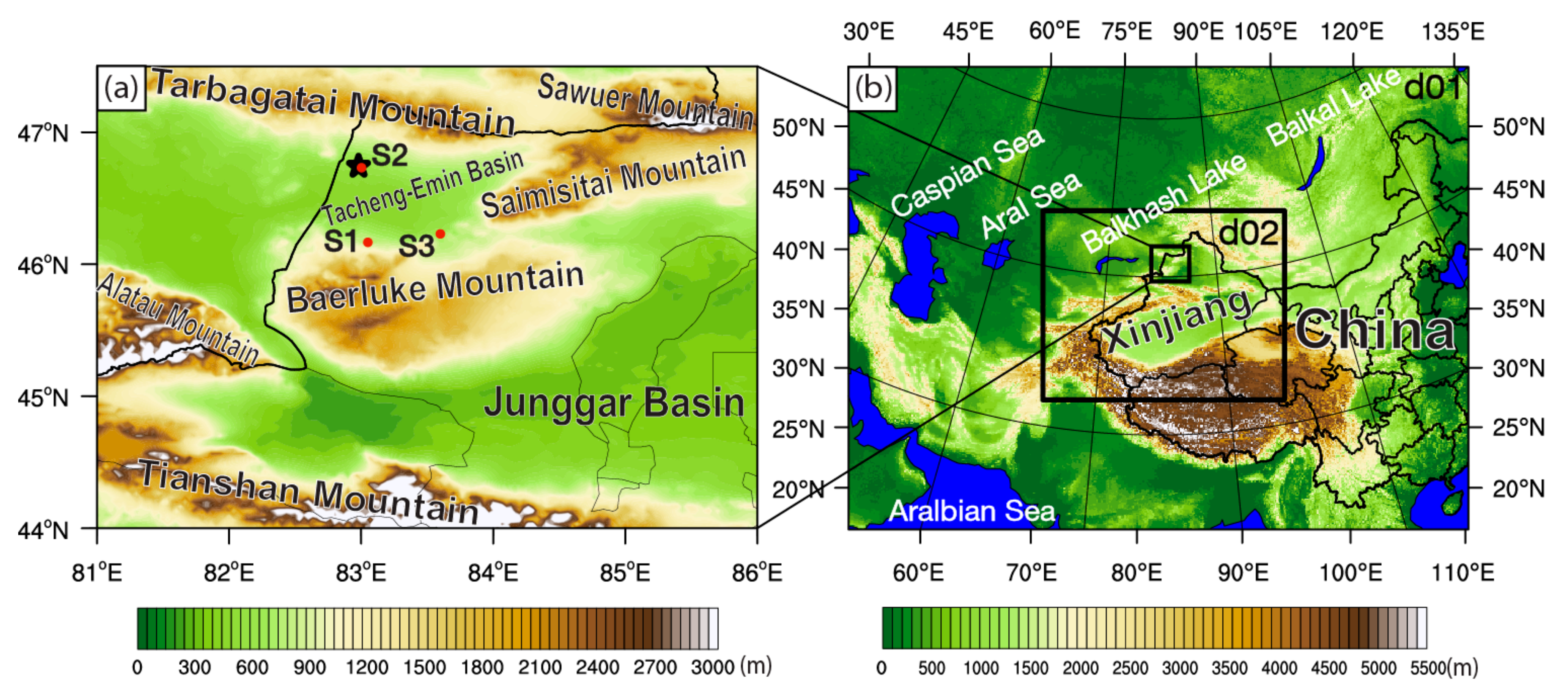
There are relatively few in-depth studies on winter snowstorms, especially in the Tacheng region of northern Xinjiang, in contrast to the relatively extensive and in-depth studies on summer precipitation both in the mid-eastern part of China and Xinjiang [44,45,46,47]. Consequently, the mechanisms of the snowstorms in northern Xinjiang are poorly understood. Furthermore, to the authors’ knowledge, systematic and in-depth research on the occurrence and development of snowstorms based on high tempo-spatial resolution and numerical simulation is absent, especially for snowstorms associated with multiple aspects such as cold fronts, low-level jets, and unstable energy over mountainous regions. The purpose of this study is to explore the mechanisms of snowstorms associated with low-level cold fronts, low-level westerly jets, and unstable energy in the western mountainous region of the Junggar Basin, Xinjiang, Northwest China, using a high-resolution numerical simulation.

The rest of this paper is organized as follows. Section 2 provides a brief overview of the snowstorms, and Section 3 presents the setup of the numerical simulation and evaluation. The mechanisms of snowstorms are analyzed in detail in Section 4. Finally, a summary and discussion are presented in Section 5. All abbreviations appearing in this article and their explanations are shown in

Table 1. List of the abbreviations and their explanations used in this study.

Abbreviations	Explanation
AGL	Above Ground Level
ASL	Above Sea Level
UTC	Universal Time Coordinated
WRF	Weather Research and Forecasting model
LLCF	Low-level Cold Front
LLWJ	Low-level Westerly Jet
MPV	Moist Potential Vorticity
CI	Convective Instability
II	Inertial Instability
HGω	Horizontal Gradient of vertical velocity
HGθe	Horizontal Gradient of the equivalent potential temperature
VSHW	Vertical Shear of the Horizontal Wind
HHV	Hybrid effect of HGθe and VSHW
Ft	Frontogenesis function

.

2. Case Overview

A severe snowstorm occurred in northern Xinjiang, Northwest China, on 22 January 2021. A total of 128 stations observed snowfall during this snowstorm event. Among them, 28 stations had moderate snow, 17 stations had heavy snow, 7 stations had very heavy snow (i.e., reaching 12.1 mm), and the heaviest snow was 19.2 mm (the snowfall intensities mentioned in this study indicate snow water equivalent value. According to the local precipitation level classification criteria of Xinjiang, the snowstorm was defined as the snow water equivalent values ranging from 12.1 mm day 1 to 24.0 mm day 1). In addition, the daily snowfall of four stations broke the record of historical extreme values in January. The areas that this article focuses on are shown in Figure 1a.

2.1. Environmental Conditions

The dataset utilized in the present study included observational data from the Fengyun-4A meteorological satellite (FY-4A), ground-based automatic stations (with a temporal resolution of 1 h), and the balloon sounding observation data. All of these observation data were provided by the National Meteorological Center of the China Meteorological Administration. In addition, the fifth-generation European Centre for Medium-Range Weather Forecasts (ECMWF) atmospheric reanalysis (ERA5) data and six-hourly, 1° × 1° gridded National Centers for Environmental Prediction (NCEP) Final (FNL) reanalysis dataset (https://rda.ucar.edu/datasets/ds083.2/, accessed on 11 April 2021) were also used.

In order to investigate the environmental conditions of this snowstorm event, the ERA5 data were used to further analyze the dynamic, thermal, and moisture conditions at 500 and 700 hPa. There was a relatively deep cold vortex at 500 hPa over the area to the north of Baikal Lake, and the western Siberia region was affected by the low vortex at 00 UTC on 22 January. At 6 UTC (Figure 2a), a relatively deep trough extending from the low vortex (indicated by “L”) oriented roughly in an east–west direction. It was located over a broad region from western Siberia to western Russia. Furthermore, another short-wave trough oriented in a north–south direction occurred over the area to the east of the Areal Sea. An upper-level jet (ULJ), reaching 40 m s⁻¹ at 300 hPa, appeared ahead of the short-wave trough (i.e., between the short-wave trough and study area), along with another ULJ located to the north of the study area. The study area was dominated by relatively weak westerlies with wind speeds of ~14–16 m s⁻¹. By 12 UTC (Figure 2b), the deep trough oriented in the east–west direction slightly moved southward, with the short-wave trough also moving eastward to some extent. Meanwhile, the northern core region of the ULJ ahead of the short-wave trough moved significantly eastward and was located near the northwestern edge of the study area, delivering more southwesterlies to the study area. At this time, the study area was roughly located under the right side of the entrance region of the ULJ, indicating that an upper-level divergence occurred over the study area.

The lower troposphere at 700 hPa at 6 UTC (Figure 2c) showed that there was a strong low-level jet (LLJ) to the northwest of the study area, with relatively weak (~4 m s⁻¹–12 m s⁻¹) southwesterlies that dominated the study area. There was a large zonal region with a relatively high horizontal gradient of potential temperature (θ) on the northwestern side of the LLJ (Figure 2e). In addition, there were three relatively weak water vapor flux convergence belts extending from the region of high θ gradient to the northwest and west of the study area, showing an orientation of roughly north–south direction. By 12 UTC (Figure 2d), the LLJ significantly moved eastward, entered the northwestern part of the study area, and brought an intense LLWJ with a horizontal wind speed reaching ~26 m s⁻¹. The entrance region of the LLWJ to the northwestern part of the study area was in good agreement with the occurrence of the LLWJ observed by the AWSs, as shown in Figure 3 and Figure 4. At this time (Figure 2f), a zonal area with a high potential temperature gradient and high water vapor flux convergence occurred near Baerluke Mountain and Saimisitai Mountain (indicated by a red arrow), revealing the arrival of the leading edge of the cold front. This cold front, along with the LLWJ, was the leading edge of an eastward-moving surface cold high. Consequently, it can be inferred that this cold front induced a relatively intense advection of cold air and moisture to the study area, and it had a rather intense LLWJ behind and ULJ above. These characteristics of the cold front were quite favorable for the formation and development of the snowstorm.

2.2. System Evolution

It can be seen from the tempo-spatial evaluation of the temperature of the black body (TBB) on top of the snowstorm clouds that there is a meso-α scale baroclinic leaf cloud system with a TBB ≤ −52 °C, mainly located over the area to the west of Xinjiang (approximately over Kazakhstan and Kyrgyzstan), showing a distribution along the northeast-southwest direction (Figure 3a). Relatively intense (TBB ≤ −61 °C) clouds mainly occurred in the northern part of the cloud system, while some other small cloud clusters in the mid-eastern part reached the same intensity. At this time, two meso-β scale banded clouds (indicated by two red arrows) developed on the eastern side of the cloud system and were roughly located over the western Tian Shan Mountains and Ili River Valley. Subsequently, the eastern part of the cloud system moved eastward, along with some other new cloud clusters developed over the area to the north (i.e., the mid-northwestern part of the study area). At 11 UTC (Figure 3b), major intense snowstorm clouds (TBB ≤ −61 °C) occurred over the study area (especially over the western mountainous region in the Junggar Basin) and near the border region between China and Kazakhstan. Over time, snowstorm clouds further intensified (TBB ≤ −64 °C) and maintained over the northwestern and mid-northern parts of the study area. Meanwhile, the cloud system further moved eastward and also developed over eastern Kazakhstan, as well as in southwestern and northwestern Xinjiang (Figure 3c). The mesoscale snowstorm clouds with TBB ≤ −64 °C lasted for ~6 h over the western mountainous region in the Junggar Basin, and their strongest period was 11–14 UTC. By 17 UTC (Figure 3d), the major intense (TBB ≤ −61 °C) part of the cloud system moved northward to some extent, and the clouds in the study area weakened significantly, resulting in a significant decay of the snowstorm in the western mountainous region of the Junggar Basin.

In addition to the heavy snowfall, the present snowstorm event was accompanied by severe high winds near the ground. According to the observations of the ground-based automatic weather stations (AWSs) in the study area, the near-surface wind in the western Junggar Basin was relatively weak (<5 m s⁻¹) at 8 UTC (Figure 4a). In contrast, the wind in the Tacheng-Emin Basin was relatively higher, especially near the northern slope of Baerluke Mountain. Two AWSs located near the northern slope of Baerluke Mountain showed higher winds (i.e., 13.2 m s⁻¹ and 16.3 m s⁻¹, respectively). These two AWSs were located close to the western portion of the canyon between Baerluke Mountain and Saimisitai Mountain. Therefore, the higher winds probably occurred due to the funneling effect (also called the canyon effect or canalization). Another AWS observed a higher wind >12 m s⁻¹ located at the northwestern bulgy edge of Baerluke Mountain. The higher wind at this AWS may have been due to the spatial edge topography.

By 11 UTC (Figure 4b), the near-surface winds in the Tacheng-Emin Basin strengthened significantly (most of the observed wind speeds were in the range from ~12.1 m s⁻¹ to 22.8 m s⁻¹), and most of the wind directions were westerlies, indicating the entrance of a strong low-level westerly jet (LLWJ). The other three AWSs located over the eastern and southeastern slopes of Baerluke Mountain also showed similar westerly (or northwesterly) high winds and one of them observed a high wind of up to 30.9 m s⁻¹, while the winds in the Junggar Basin were still weak (<5 m s⁻¹).

At 14 UTC (Figure 4c), the high winds in the Tacheng-Emin Basin further strengthened (most of the observed wind speeds ranged from ~16.7 m s⁻¹ to 23.7 m s⁻¹), and the wind directions roughly remained as westerlies, showing the further intensification of the LLWJ. At this time, the aforementioned three AWSs located over the eastern and southeastern slopes of Baerluke Mountain observed higher wind speeds, and one of them showed a high wind of up to 40.7 m s⁻¹. The winds in the Junggar Basin remained relatively weak (most wind speeds were <8 m s⁻¹). However, an AWS located over the southern portion of the canyon between Alatau Mountain and Baerluke Mountain observed a higher wind of 23.6 m s⁻¹. By 17 UTC (Figure 4d), the wind speed observed by most of the AWSs located over the northwestern part of the Junggar Basin also showed the influence of the LLWJ, showing a significant increase in the wind speed (reaching ~29.2 m s⁻¹).

In order to investigate the evolution of basic meteorological elements during the snowstorm event, we selected three AWSs in the Tacheng-Emin Basin (as shown as S1, S2, and S3 in Figure 1a) for further analysis. As shown in Figure 5a, precipitation began to be observed at station S1 at 11 UTC, which reached a relatively high value of >2.5 mm during 13–14 UTC, and then it gradually decreased in the period between 15 and 19 UTC. It is clear that other basic meteorological elements significantly changed before the occurrence of the snowfall. For example, the wind speed increased significantly during 7–11 UTC, especially showing a sharp increase (from ~4 m s⁻¹ to ~19 m s⁻¹) during 7–10 UTC, while the wind direction changed from northwesterly to westerly during 9–10 UTC. In addition, the relative humidity (RH) increased from 58% to 89% during 9–11 UTC. Furthermore, the temperature decreased monotonously from ~2 °C to ~−14 °C from 9 UTC on 22 January to 4 UTC on 23 January, and the sharpest temperature drop (~7 °C) occurred during 9–14 UTC on 22 January (i.e., before the occurrence of the heaviest snowfall observed by S1). Moreover, the pressure also showed a significant monotonous increasing trend from 7 UTC on 22 January to 2 UTC on 23 January, and the pressure jump was up to ~35 hPa. The significant abrupt changes in wind speed, wind direction, and relative humidity, as well as the monotonous temperature drop and pressure jump, indicate the passage of a cold front accompanied by moist air and the LLWJ.

For station S2 (Figure 5b), precipitation occurred during the period from 13 to 18 UTC. The wind speed increased significantly (from ~5 m s⁻¹ to ~17 m s⁻¹) during 9–12 UTC, while the wind direction changed sharply from southerly to westerly during 9–10 UTC. The RH increased obviously from ~61% to ~80% during 9–11 UTC, and a temperature drop of ~5 °C (from ~3 °C to ~−2 °C) was observed in this 2 h period as well. At a later stage from 12 UTC on 22 January to 00 UTC on 23 January, the temperature decreased monotonously, showing a relatively slight decreasing trend. Furthermore, the pressure began to increase after 7 UTC on 22 January, and also monotonously increased during the period in the coming 20 h, showing the same pressure jump (~35 hPa) as S1. The overall change patterns of the elements observed at these two stations were similar. However, the beginning times of the significant change in some elements at S2 were ~2 h later than that of S1. This time lag reveals that the cold front affected S2 later than S1, which was likely due to the relatively southern geographical location of S2.

At station S3 (Figure 5c), precipitation occurred in almost the same time period as S2, and the evolution of the pressure was also similar to that of S2. However, the wind speed observed by S3 was significantly different from that of the other two AWSs. It maintained a relatively high value (~17 m s⁻¹) during 5–8 UTC, sharply decreased to ~7 m s⁻¹ in the period between 8 and 10 UTC, and then sharply increased up to ~23 m s⁻¹ at 11 UTC. The wind direction in the period between 5 and 9 UTC was maintained as southeasterly but sharply turned northwesterly at 1 UTC. (The high wind during the period 5–8 UTC was probably due to the funneling effect that occurred near the canyon between Baerluke Mountain and Saimisitai Mountain. A similar southeasterly high wind was also found near the region close to the S3 in Figure 4a). After 10 UTC, a significant increase in RH (from ~60% to 84%) was also observed between 10 and 11 UTC. The temperature also decreased monotonously in a 17 h period after 10 UTC. In general, almost all of the basic meteorological elements observed by the three AWSs revealed that there was a cold front accompanied by moist air, and LLWJ affected this region before the occurrence of the snowstorm.

However, the formation mechanism of the snowstorm is still unclear due to the limitations of the tempo-spatial resolution of ERA5 data and observational data. Consequently, in order to further investigate the mechanisms of the snowstorm, numerical simulations with a high tempo-spatial resolution were conducted as follows.

3. Numerical Simulation

3.1. Setup of Numerical Experiment

The numerical simulation was performed using the Weather Research and Forecasting (WRF) model (V4.2.1) [48], with two-way nested two-level domains and horizontal grid spacings of 9 km and 3 km, respectively (Figure 1b). The inner domain fully covered the whole of Xinjiang and some of the upstream areas. For both domains, the model physics adopted the WRF Single Moment 6-class (WSM6) microphysics scheme [49], YSU (Yonsei University) planetary boundary layer scheme [49,50], Unified Noah land surface model scheme [51], Rapid Radiative Transfer Model for GCMs (RRTMG) longwave and shortwave radiation schemes [52], and Revised MM5 (Fifth-Generation Penn State/National Center for Atmospheric Research Mesoscale Model) Monin–Obukhov scheme [50]. The Kain–Fritsch scheme [53] (Kain 2004) was used for cumulus parameterization in domain d01, whereas it was turned off in domain d02. (Above physical parameterization schemes were selected as the most appropriate combination based on the results of a dozen numerical experiments.) The initial and boundary conditions for the simulation were created using the six-hourly NCEP FNL analysis data with a resolution of 1° × 1°. All domains were initialized at 6 UTC on 22 January 2021 and integrated for 30 h. The time intervals of the output data of d01 and d02 were 60 min and 10 min, respectively.

3.2. Evaluation of Simulation

In order to establish the credibility of the simulation, the simulated 24 h accumulated precipitation and atmospheric stratification conditions (indicated by the Skew T-logP diagram) were compared to their observational counterparts. The observed 24 h accumulated precipitation was obtained by AWSs, and the interpolated distribution patterns of the precipitation were unsatisfactory due to the heterogeneous distribution of the AWSs in the study area. Several common interpolation methods were tried, such as inverse distance weighted interpolation, Cressman Interpolation, natural neighbor interpolation, and tension splines interpolation). Therefore, different colorful symbols are used to represent the intensity of the accumulated precipitation at each station. As shown in Figure 6a, three high precipitation areas (indicated by black dashed ellipses) can be identified according to the observed 24 h accumulated precipitation pattern in northwestern Xinjiang. The northwestern high precipitation area is located over the western mountainous region of the Junggar Basin (i.e., mainly near the Baerluke Mountain), whereas the southwestern and southeastern high precipitation areas are located over the Ili River Valley (including the mountainous region on both sides) and the northern slope of the Tian Shan Mountains, respectively. The overall pattern of the simulated 24 h accumulated precipitation (Figure 6b) also roughly showed three similar high precipitation areas (also denoted by black dashed ellipses) located over the same regions, which is generally consistent with the observations.

The atmospheric stratification conditions at 00 UTC on 22 January observed by balloon sounding at Tacheng weather station indicated that there were two obvious thermal inversion levels at the lower level below ~800 hPa. At the lowest inversion level, the temperature increased from −4.5 °C (at 943.5 hPa, i.e., the lowest level) to 3.5 °C (at 910 hPa). For the other relatively thinner inversion level, the temperature increased from −0.8 °C (at 837 hPa) to 1.5 °C (at 801 hPa). This type of inversion level indicates a significant stable stratification that suppresses the local ascending flow. The low level below 850 hPa was dominated by weak easterlies (<12 m s⁻¹), whereas some moderate westerlies (~16–18 m s⁻¹) occurred at the levels between 400 hPa and 500 hPa. The dewpoint depression (T-Td) was ~4.5 °C near the surface, and it gradually increased with height, showing a rather dry air (dewpoint depression reaching ~21 °C) at ~740 hPa. Humidity gradually increased with height, showing relatively moist air (dewpoint depression reaching ~6 °C) at ~500 hPa. However, the air at the upper level became rather dry again, and the dewpoint depression reached ~27 °C at ~440 hPa.

By 12 UTC (Figure 7a), the thermal, dynamic, and moisture characteristics of the stratification conditions notably changed. For example, the aforementioned thermal inversion layers weakened significantly and almost disappeared, showing a roughly neutral thermal stratification in the low layer from 925 to 890 hPa and another neutral thermal stratification layer from ~800 hPa to ~700 hPa, with small temperature perturbation. The disappearance of the thermal inversion layers was favorable for the release of some unstable energies and the occurrence of some local ascending flows. Furthermore, the wind speed at low levels below 850 hPa increased remarkably, showing a west-northwesterly high wind reaching ~24 m s⁻¹ at 890 hPa. This high wind coincided with the LLWJ analyzed above (Figure 3 and Figure 4). In contrast, a relatively weak (~12 m s⁻¹) west-northwesterly wind occurred at ~800 hPa, along with a west-southwesterly wind reaching ~16 m s⁻¹ at ~600 hPa. This type of anti-cyclonic vertical shear in the horizontal wind direction indicates that there was a cold advection in the layer between 800 hPa and 600 hPa. The wind speed increased significantly with height above 500 hPa and almost reached the intensity of a typical upper-level jet (~30 m s⁻¹) at the level between ~400 hPa and 300 hPa. Meanwhile, the basic Skew T-logP diagram parameters showed that the pressure and temperature of the lifting condensation level (LFC) were 907 hPa and −4 °C, respectively. The precipitable water was ~8 mm, and there was no convective available potential energy (CAPE).

At this time, the simulated stratification conditions (Figure 7b) showed that there were two neutral thermal stratification layers occurring in the near-surface layer below ~880 hPa and the layer between ~800 hPa and ~700 hPa, which was in good agreement with the observations. However, the level below ~650 hPa was rather wet (dewpoint depression reaching <3 °C), especially at low levels below 850 hPa (dewpoint depression reaching <~1 °C). In addition, the vertical wind profile shows that there was a westerly high wind reaching ~28 m s⁻¹ at ~880 hPa, along with a significant anti-cyclonic vertical shear of horizontal wind direction occurring in the layer between ~800 hPa and ~600 hPa, denoting cold advection. Additionally, the upper level above ~400–300 hPa was dominated by southwesterly high winds (reaching ~30 m s⁻¹). These wind characteristics were also in good agreement with the observations.

In general, the precipitation distribution (indicating the basic characteristics of the occurrence and development of the snowstorm system), thermal, dynamic, and moisture characteristics of the stratification conditions in the simulation agreed well with their observational counterparts. Therefore, the simulation results were considered reliable for further analysis of the snowstorm mechanism based on the WRF simulation data with 3 km resolution, as discussed in the following section.

4. Mechanism of the Snowstorm

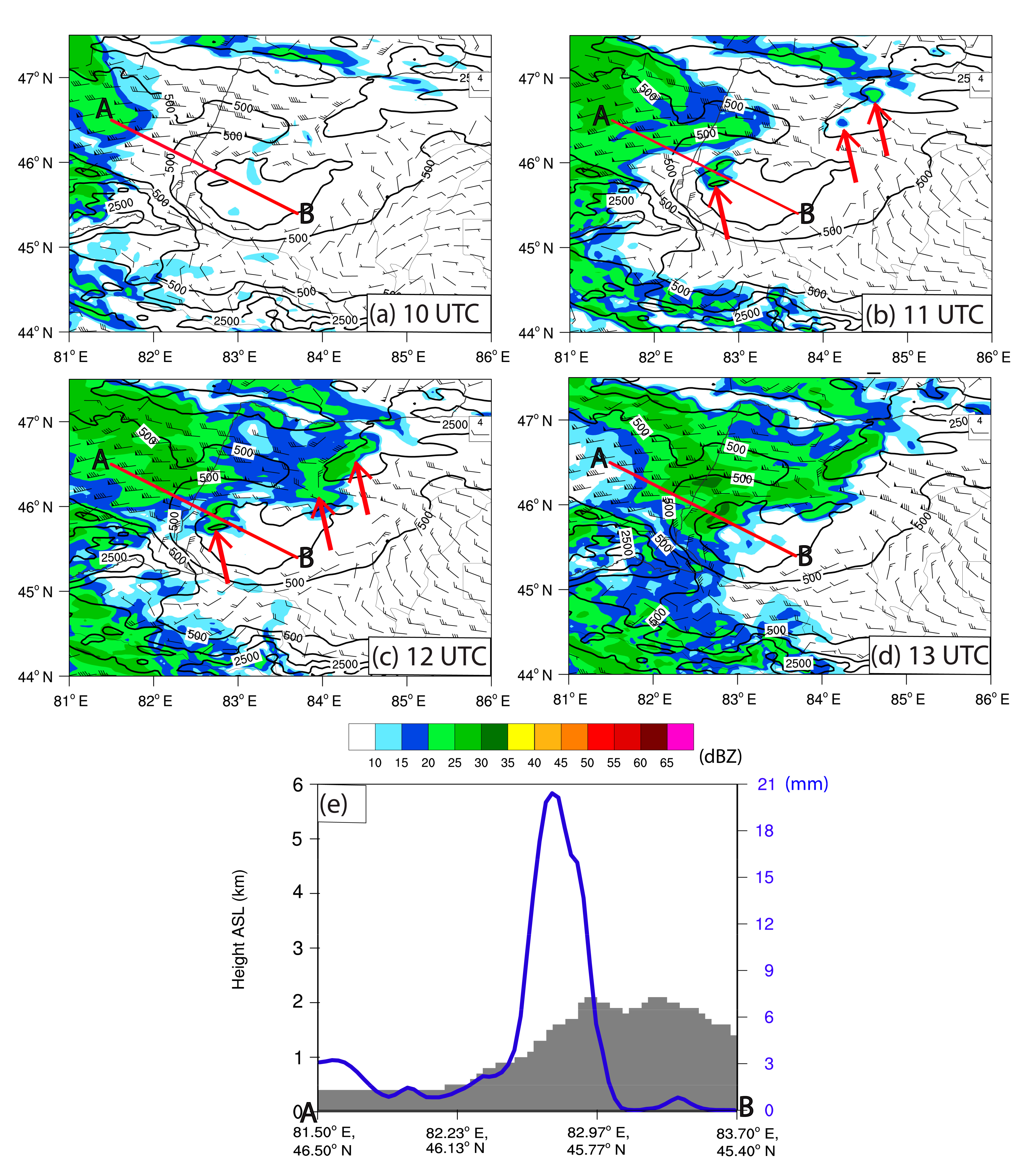
Figure 8 shows the hourly evolution of the simulated composed radar reflectivity during the occurrence and development of the snowstorm in the western mountainous region of the Junggar Basin. At 10 UTC (Figure 8a), the snowfall cloud clusters formed roughly over the area to the west of the study area (i.e., Kazakhstan) and were moving eastward. At about 11 UTC (Figure 8b), the eastward-moving snowfall clouds further moved over the Tacheng-Emin Basin, and some other local snowfall cloud clusters were initiated locally over the windward slope (i.e., northwestern slope) of Baerluke Mountain and Saimisitai Mountain (indicated by red arrows). By 12 UTC (Figure 8c), locally initiated snowfall cloud clusters continuously occurred and developed (denoted by red arrows) on the windward slope area of the mountainous area, and eventually merged with the eastward moving snowfall clouds. At about 13 UTC (Figure 8d), the intensity of the composed reflectivity of the merged snowfall clouds was further strengthened, forming a relatively intense and wide snowfall cloud system over the Tacheng-Emin Basin and the windward slope of the mountains. During the coming ~4 h period, the merged snowfall clouds maintained an intense status, mainly over the northwestern windward slope of the mountainous region, resulting in the local snowstorm mentioned above (i.e., Figure 6). The 24 h accumulated precipitation variation along line AB (Figure 8e) shows that the major precipitation mainly occurred over the upper half of the windward slope of Baerluke Mountain, whereas there was little precipitation over the mountain peak. This was probably due to a quasi-stationary downdraft with an intensity of ~1 m s⁻¹, which was probably generated due to the orographic GWs. As mentioned by Li et al., 2021 [34], GWs usually show a flow pattern in the form of alternatively distributed rising and sinking motions over the mountains.

In general, the snowstorm event was mainly caused by the merging and enhancement of the eastward-moving snowfall clouds and the locally induced snowfall clouds over the windward slope of the mountains, as well as the ~4 h maintenance of the post-merger snowfall clouds over the western mountainous region of the Junggar Basin.

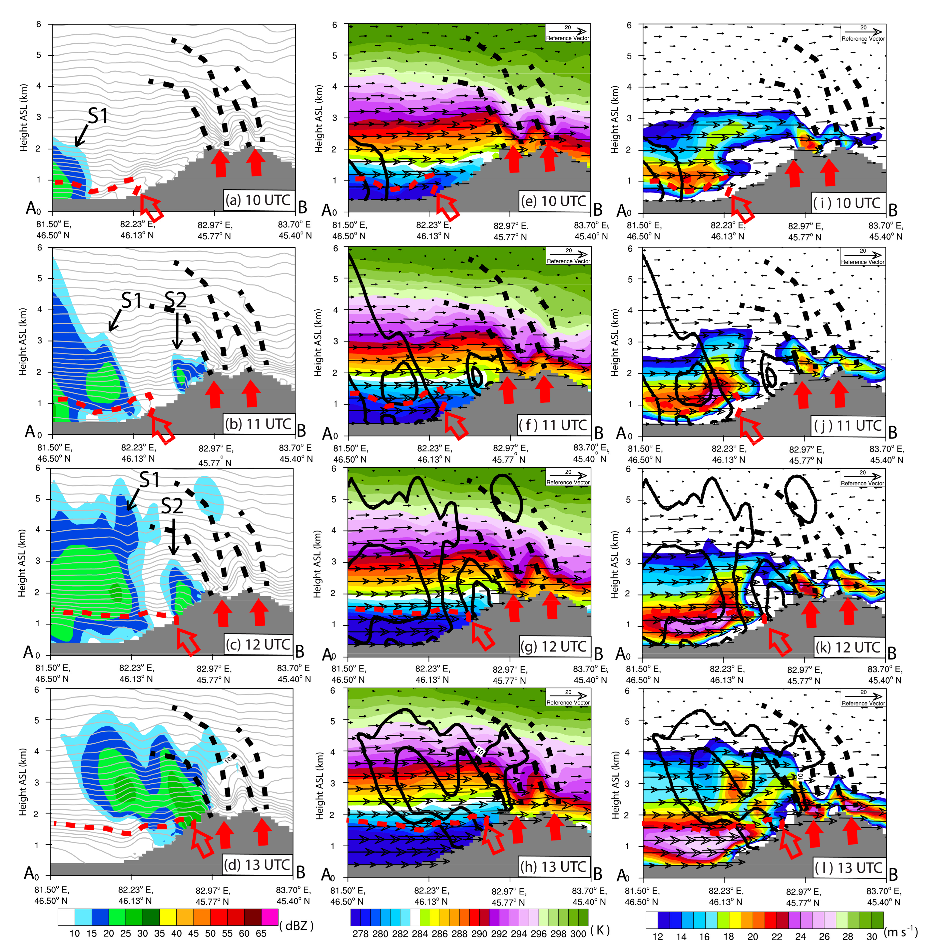
Figure 9 shows the tempo-spatial characteristics of the composed reflectivity, potential temperature (θ), and horizontal wind speed on the vertical cross-section along the line AB during the initiation and significant development period (i.e., 10–13 UTC) of the snowfall clouds near Baerluke Mountain. At 10 UTC (Figure 9a,e,i), a snowfall cloud (labeled as S1) accompanied by an eastward moving LLCF (indicated by the red dashed line) and LLWJ (also analyzed in the AWS observations in Figure 3 and Figure 4) entered the plain region located northwest of Baerluke Mountain. It can be inferred from the vertical distribution of θ that the minimum value within the LLCF reached about 276 K. The 280 K isotherm showed an obvious protruding forward (“nose-like”) pattern near the foot of Baerluke Mountain (Figure 9a,e). Furthermore, the highest horizontal wind speed in the LLWJ reached ~20 m s⁻¹. The major portion of the LLWJ occurred at a low level below 2000 m ASL, and the maximum wind speed center was located around 1000 m ASL. Meanwhile, there were two distinct areas where the isotherms bent downward significantly (exhibiting a nearly vertical distribution) above the two peaks of Baerluke Mountain. The isotherms in these areas were obviously denser than those in other areas, which reflected a relatively larger horizontal temperature gradient at these locations. Therefore, it can be inferred that two cold fronts (surrounded by the double black dashed lines) were also present above these two peaks (the locations of these two cold fronts are denoted by the two filled red arrows). In addition, there were two high wind areas at low levels below 3 km ASL over the mountain peaks. These types of thermal and dynamic disturbances were probably generated due to alternatively distributed rising and sinking motions induced by the aforementioned orographic GWs above the mountain. However, these orographic cold fronts are not our interest in this paper, and there were few precipitations that occurred over the mountain peak. Therefore, the characteristics of all quantities that will be analyzed below the mountain peak will not be considered.

By 11 UTC (shown in Figure 9b,f,j), the S1 and accompanied LLCF further moved toward the windward slope of Baerluke Mountain, and S2 began to form in the upper part of the windward slope. The LLWJ further intensified with its central maximum wind speed exceeding 23 m s⁻¹. This time was selected for representing the early stages of the occurrence and development of the snowfall clouds.

Over time, at 12 UTC (Figure 9c,g,k) and 13 UTC (Figure 9d,h,l), the snowfall clouds merged and underwent further development. Therefore, 13 UTC was selected for representing the later stage of the merging and further development of the snowfall clouds. During this period, the LLCF and accompanying LLWJ gradually intensified, moved further eastward, and were mainly located over the upper-middle part of the windward slope. The merged snowfall clouds were maintained for about 3 h in the later stage, mainly above the windward slope of the mountain.

In order to investigate the mechanisms of the occurrence and development of the snowfall clouds, the moist potential vorticity (MPV) was calculated and analyzed.

The moist potential vorticity (MPV) is a useful physical quantity that is frequently used in diagnosing mid-latitude heavy precipitation [34,39,54,55,56,57,58]. MPV can simultaneously reflect the combined effects of atmospheric moisture, and thermal and dynamic features [34,39,54,56,57,59,60]. Moreover, MPV can also indicate the characteristics of atmospheric instability, and it has been used in the study of snowstorms in recent years [34,41,54]. We calculated and analyzed the MPV near the windward slope of Baerluke Mountain in order to investigate the occurrence and development mechanisms of the snowstorm. According to previous studies [39,43,55,61], the MPV in the p-coordinate system is expressed as follows:

$$\mathrm{MPV}=-\mathrm{g}\left({\xi }_p+f\right)\frac{\partial {\theta }_e}{\partial p}+\mathrm{g}\frac{\partial v}{\partial p}\frac{\partial {\theta }_e}{\partial x}-\mathrm{g}\frac{\partial u}{\partial p}\frac{\partial {\theta }_e}{\partial y}$$

(1)

where, g is the acceleration of gravity, ${\xi }_p$ is the relative vertical vorticity, $f$ is the Coriolis parameter, p is the pressure, ${\theta }_e$ is the equivalent potential temperature, and $v$ and $u$ are the horizontal wind components in $x$ and $y$ directions, respectively. According to some previous studies related to MPV [31,41,43,62], the first term on the right-hand side of Equation (1) is the barotropic component of the MPV (also called the vertical component of the MPV, abbreviated as MPV1), reflecting the combined effect of absolute vorticity (${\xi }_p+f<0$ indicates inertial instability, II) and $\partial {\theta }_e/\partial p$ (represents convective instability, CI). The second term on the right-hand side of Equation (1) is the baroclinic component of the MPV (abbreviated as MPV2, which is also called the horizontal component of the MPV), indicating the contribution of the horizontal gradient of the equivalent potential temperature ($\mathrm{HG}{\theta }_e$) and the vertical shear of the horizontal wind (VSHW). These two components of the MPV are composed as follows:

$$\mathrm{MPV}1=-\mathrm{g}\left({\xi }_p+f\right)\frac{\partial {\theta }_e}{\partial p}$$

(2)

$$\mathrm{MPV}2=\mathrm{g}\frac{\partial v}{\partial p}\frac{\partial {\theta }_e}{\partial x}-\mathrm{g}\frac{\partial u}{\partial p}\frac{\partial {\theta }_e}{\partial y}$$

(3)

The negative MPV often indicates atmospheric instability in some diagnostic analyses on mid-latitude heavy precipitation events, especially in extratropical cyclone/frontal systems [34,54,55,56,57,58,61]. Consequently, we investigated the tempo-spatial evolutions of the negative MPV during the occurrence and development of snowstorm clouds over the windward slope of Baerluke Mountain.

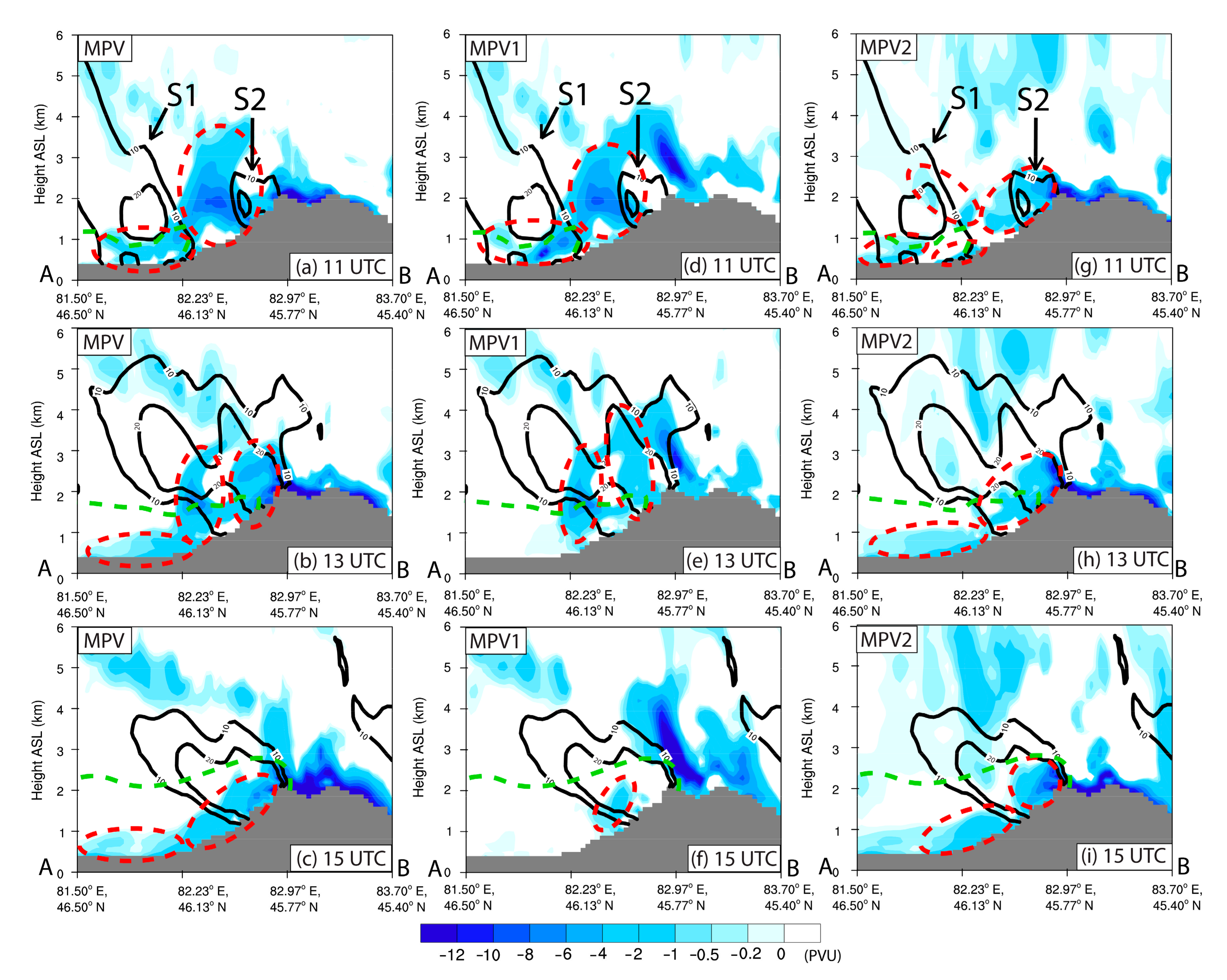
At the early stage (i.e., 11 UTC, Figure 10a), two major negative MPV areas were observed over the plane region and windward slope (indicated by the two red dashed ellipses). The negative MPV area located over the plain region was relatively weak, and its vertical extent was about 1–1.5 km above sea level (ASL), located within the lower part of S1. Another relatively larger negative MPV area (intensity reaching about −6 PVU) over the windward slope had a vertical extent up to ~4 km ASL, with the strongest center located at ~2 km ASL over the intermediate region between S1 and S2. At the later stage (i.e., 13 UTC, Figure 10b), the negative MPV area in the plain region weakened to some extent and decreased significantly to a vertical extent. The negative MPV area above the windward slope was divided into two parts (shown by the two red dashed ellipses) and they were roughly located below the two intense composed reflectivity centers (>20 dBZ) of the merged snowstorm cloud. Over time, the intensity and vertical extent of the negative MPV area further weakened and reduced to some extent (i.e., 15 UTC, Figure 10c).

In general, a relatively intense negative MPV reflecting the corresponding atmospheric instabilities appeared below and near S1 and S2 and in the intermediate region between them at the early stage. However, the extent and (or) intensity of the unstable layer, which was reflected by the negative MPV below the snowstorm clouds decreased, with the development of the snowstorm clouds at a later stage, which was an indication of the release of the corresponding unstable energy. During the much later, stage when the cloud system maintained for about 3 h (i.e., from 15 to 18 UTC), the unstable layer below the clouds also remained for almost the same time. However, the intensity of the unstable layer reflected by the negative MPV was weaker than that of the previous stages when the clouds occurred, merged, and significantly developed. In order to further understand the specific instability characteristics reflected by the negative MPV, two components of the MPV (shown in Equations (2) and (3)) were also analyzed.

At the early stage (Figure 10d), the intensity and vertical extent of the MPV1 (indicated by the larger red dashed ellipses) were almost the same as that of the negative MPV area over the plane region and windward slope, respectively (shown in Figure 10a). Specifically, although the distribution characteristics of the MPV1 within S1 in the lower altitude below ~1 km ASL were found to be roughly similar in extent to the corresponding negative MPV area, the MPV1 was more intense than the MPV at the lower level within the LLCF near the foot of Baerluke Mountain (shown in the smaller red dashed ellipse). However, the MPV2 within and near S1 was rather weak (Figure 10g, shown by three red dashed ellipses over the plain region). In contrast, the MPV2 over the middle to the upper part of the windward slope was rather intense and mainly occurred at a relatively shallower level below ~1.5 km above ground level (AGL) (denoted by the largest red dashed ellipse).

At a later stage (Figure 10e,h), the overall intensity of the MPV1 decreased to some extent with the merging and further development of S1 and S2. The MPV1 over the plain region disappeared, while there were two MPV1 centers over the windward slope roughly below the main body of the merged snowfall cloud. One of them was at the level of ~1–3 km ASL, and the other was located over the upper half of the windward slope at the level of ~1.5–4 km ASL. In contrast, the MPV2 at the lower level below ~1 km ASL over the plane region intensified to some extent. In addition, the MPV2 in the lower level below ~1.5 km AGL above the middle to the upper part of the windward slope still maintained a relatively intense value (almost the same intensity as that of the early stage).

By 15 UTC (Figure 10f,i), the MPV1 over the windward slope was sharply reduced, leaving only a very small area showing MPV1 (shown by the small red dashed ellipse in Figure 10f). However, the MPV2 still showed an almost similar intensity as the previous stage as a whole. The MPV2 area, previously located over the plain region, further moved upslope and was located roughly over the lower half of the windward slope. The other MPV2 area was still located over the upper part of the windward slope and had a relatively intense value reaching −10 PVU.

In general, at the early stage, the major instability was mainly dominated by the MPV1, while the MPV2 had some significant contributions mainly at the lower level below ~1.5 km AGL over the upper part of the windward slope. At the later stage, although the MPV1 decreased to some extent as a whole, it still had a major contribution in the mid-lower level (from ~1 km to 3~4 km ASL) within and (or) below the major part of the merged snowfall cloud. The MPV2 still played an important role at the low level below ~1.5 km AGL over the windward slope. During the much later period (15 UTC), the MPV1 had almost been released, while the MPV2 still provided a significant contribution over the windward slope, and supported the snowfall clouds to be maintained for several hours.

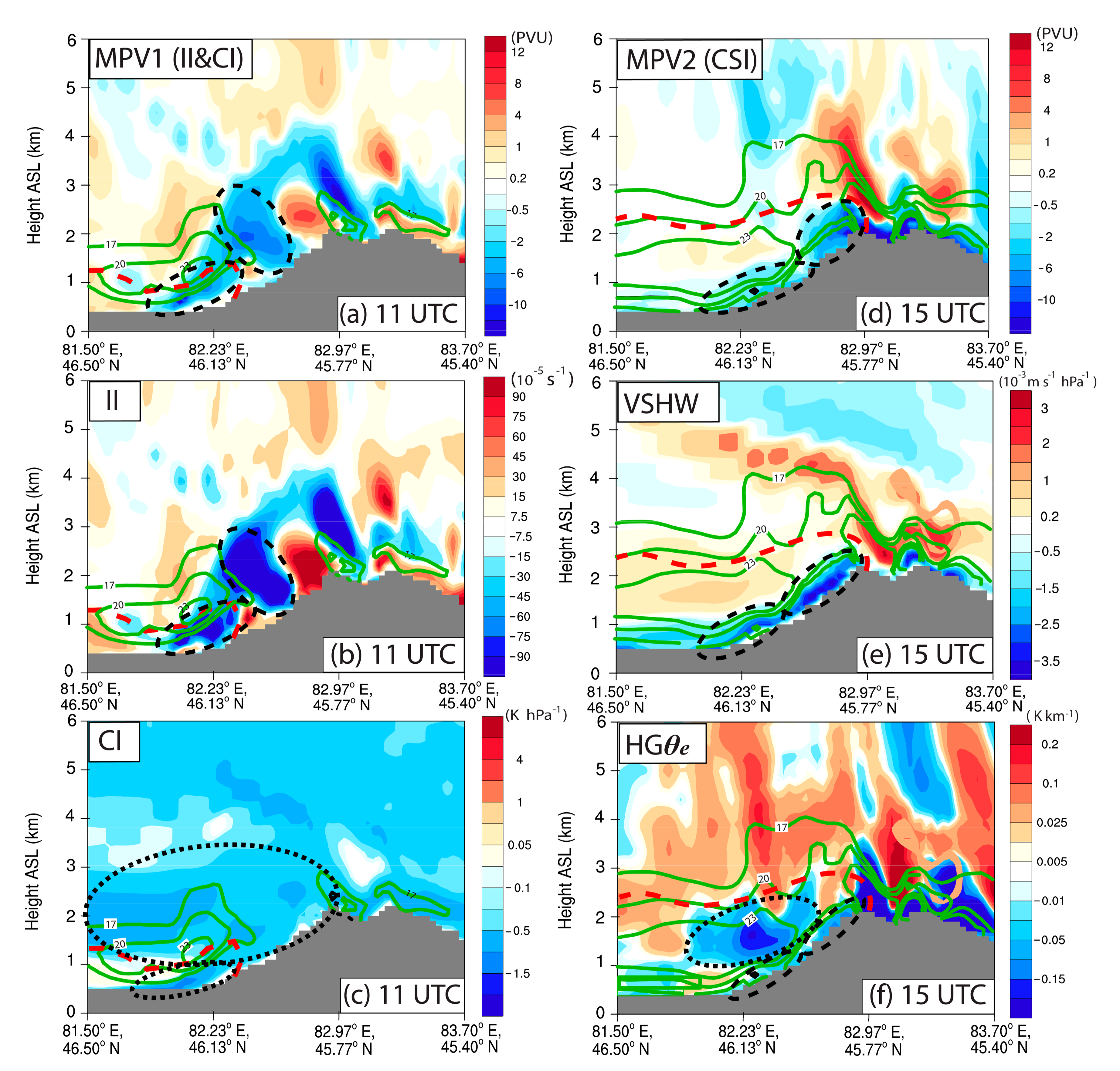
In order to further understand the intuitional physical process of the instabilities mentioned above, specific factors that mainly influence the MPV1 and MPV2 were further analyzed. At the early stage (Figure 11), the location and vertical extent of the two major areas of MPV1 (indicated by black dashed ellipses) were very similar to that of the II (Figure 11b). One of the high II centers was located over the middle part of the windward slope almost from the surface to the level of ~3 km ASL, which also corresponded to the leading edge (or ahead) of the LLWJ. The other was located near the foot of the mountain below ~1.2 km ASL, which corresponded to just below the core area of the jet. In contrast, the CI showed a wide-ranging area with a relatively uniform distribution above ~1 km ASL (Figure 11c, shown by the large black dotted ellipse), along with a relatively intense CI center in the LLCF near the foot of the mountain (indicated by the small black dashed ellipses). Therefore, it can be deduced that the MPV1 was mainly determined by the II that occurred in the front and below the core region of the LLWJ.

At the later stage (roughly during the period from 13 UTC to 15 UTC), the MPV2 showed a relatively intense value at a low level below ~1 km AGL over the windward slope (Figure 11d, shown in the two black dashed ellipses). The vertical shear of the horizontal wind (VSHW) also showed an intense negative value at almost the same low level below ~0.8 km AGL, mainly over the windward slope below the LLWJ (Figure 11e, indicated by the two black dashed ellipses). Meanwhile, the horizontal gradient of the equivalent potential temperature ($\mathrm{HG}{\theta }_e$) exhibited a rather weak negative value at the near-surface level below ~0.5 km AGL, along with a rather intense value at the level between ~0.5 km and 1.8 km AGL aloft (Figure 11f, denoted by the larger black dotted ellipse). However, the location of the area with a rather intense $\mathrm{HG}{\theta }_e$ was not collocated with that of the intense MPV2; therefore, it can be neglected. Consequently, it can be concluded that the MPV2 below ~1 km AGL over the windward slope was mainly contributed by the VSHW, where, the $\mathrm{HG}{\theta }_e$ had a relatively weak positive contribution at the near-surface level below ~0.5 km AGL. The high value of VSHW in the low layer was probably induced by the inhomogeneity of the momentum in the intermediate area between the LLWJ and windward slope topography. The atmospheric baroclinicity reflected by HGθe was probably attributed to the thermal inhomogeneity associated with the LLCF.

As mentioned in the introduction, the frontogenetical forcing was considered an important forcing mechanism of snowstorms. Therefore, the frontogenesis function was also calculated and analyzed to further investigate the frontogenetical forcing mechanism required for the release of the above-mentioned instabilities. Following [63,64] and Yang et al. [65], the frontogenesis function can be expressed as follows:

$$\mathrm{Ft}=\frac{\mathrm{d}}{\mathrm{d}t}\left|\nabla \theta \right|={\mathrm{F}}_1+{\mathrm{F}}_2+{\mathrm{F}}_3+{\mathrm{F}}_4$$

(4)

where, F₁, F₂, F₃, and F₄ are defined, respectively, as:

$${\mathrm{F}}_1=\frac{1}{\left|\nabla {\theta }_e\right|}\left[(\nabla {\theta }_e·\nabla )\left(\frac{d{\theta }_e}{dt}\right)\right]$$

(5)

$${\mathrm{F}}_2=-\frac{1}{2}\frac{1}{\left|\nabla {\theta }_e\right|}{\left(\nabla {\theta }_e\right)}^2\left(\frac{\partial u}{\partial x}+\frac{\partial y}{\partial y}\right)$$

(6)

$${\mathrm{F}}_3=-\frac{1}{2}\frac{1}{\left|\nabla {\theta }_e\right|}\left[{\left(\frac{\partial {\theta }_e}{\partial x}\right)}^2-{\left(\frac{\partial {\theta }_e}{\partial y}\right)}^2\right]\left(\frac{\partial u}{\partial x}-\frac{\partial v}{\partial y}\right)+2\frac{\partial {\theta }_e}{\partial x}\frac{\partial {\theta }_e}{\partial y}\left(\frac{\partial v}{\partial x}+\frac{\partial u}{\partial y}\right)$$

(7)

$${\mathrm{F}}_4=-\frac{1}{\left|\nabla {\theta }_e\right|}\left[\frac{\partial {\theta }_e}{\partial p}\left(\frac{\partial {\theta }_e}{\partial x}\frac{\partial \omega }{\partial x}+\frac{\partial {\theta }_e}{\partial y}\frac{\partial \omega }{\partial y}\right)\right]$$

(8)

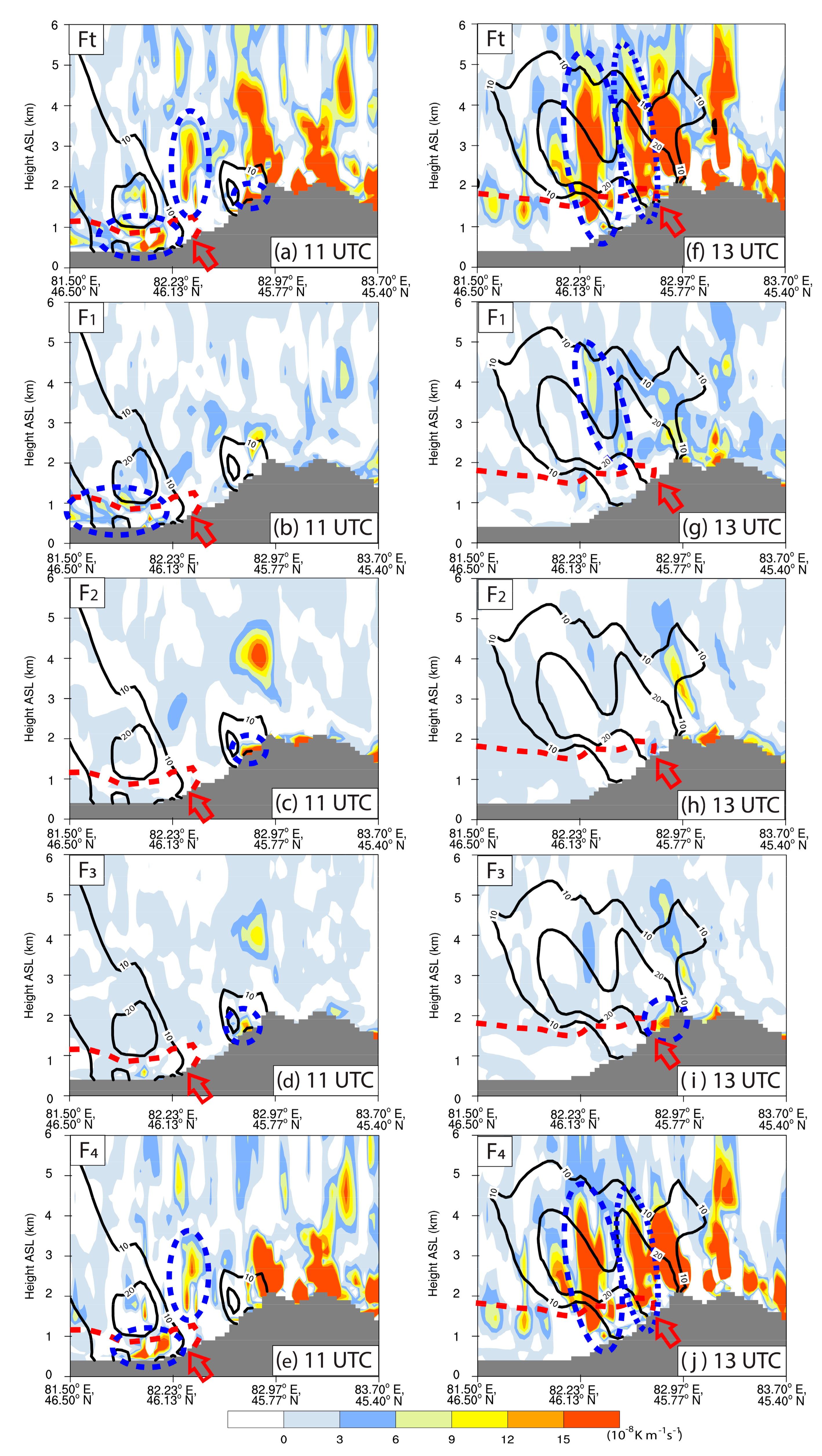
where, ${\theta }_e$ is the equivalent potential temperature, u and v are the horizontal wind components in x and y directions, respectively, and $\omega$ is the vertical velocity in the p coordinate. F₁, F₂, F₃, and F₄ represent diabatic heating, convergence, deformation, and slantwise terms, respectively. The tempo-spatial characteristics of the total value of the frontogenesis function (Ft) and its four components during the major development period of the snowfall clouds were also investigated.

At the early stage (i.e., 11 UTC), the main areas with a high value of Ft associated with the present snowstorm event were mainly located inside and below S1 and S2 and over the intermediate area between them (shown by the blue dashed ellipses in Figure 12a). The overall intensity of F₁ was rather weak, and it was mainly distributed in the area near the middle and rear of the LLCF below S1 (indicated by the blue dashed ellipse). F₂ had a high-value center at the lower level below ~0.4 km over the upper part of the windward slope below S2 (Figure 12c, shown by the blue dashed ellipse). Meanwhile, F₃ (Figure 12d) had a distribution pattern similar to that of F₂, but with an overall weaker intensity (Figure 12d). It had a high-value center at the same low level over the upper part of the windward slope (shown by the blue dashed circle). However, the overall distribution of F₄ was similar to that of Ft (Figure 12e). There were two high-value centers within the LLCF and above its leading edge at about 1.5–3.5 km ASL (shown by the blue dashed circle).

At a later stage (i.e., 13 UTC), as S1 and S2 merged and underwent significant development, Ft exhibited three high-value centers over the windward slope (shown by the three blue dashed ellipses in Figure 12f). At this time, F₁ (Figure 12g) still showed an overall weaker intensity, while a relatively high-value center occurred at the middle level (i.e., 2–5 km ASL) within the merged snowfall clouds (shown by the blue dashed circles). The distribution of F₂ (Figure 12h) showed that a previous (at 11 UTC) high-value center over the upper part of the windward slope almost disappeared at this time. The high value of F₃ (Figure 12i) mainly occurred at the low level below ~0.5 km AGL in front of the leading edge of the LLCF (shown by the blue dashed circle). Nevertheless, F₄ (Figure 12j) showed three high-value centers above the windward slope (shown by the blue dashed ellipses), which were similar to those of Ft in terms of size and intensity.

In general, Ft was mainly dominated by F₄ during the whole period of occurrence and development of the snowfall clouds. Specifically, in the early stage, except for the major dominance of F₄ in the area below the snowfall cloud S1 and the intermediate region between S1 and S2, F₁ also made relatively weak positive contributions at the low level below S1, whereas F₂ and F₃ played important roles at the lower level below ~0.4 km over the upper part of the windward slope, where it was collocated with the location of S2. In the later stage, F₁ provided a relatively weak contribution at the mid-level (i.e., 2–5 km ASL) within the merged snowfall clouds, whereas F₃ made a significant contribution at the same low level below ~0.5 km AGL over the upper part of the windward slope.

F₁ is mainly due to the latent heat released by the condensation, while F₂ and F₃ mainly resulted from the local convergence and horizontal curvature, respectively. In the present case, F₁ probably resulted from the latent heat released by condensation in the snowfall clouds, while F₂ and F₃ were probably induced by the local convergence due to the blocking effect and special protruding shape of the windward slope of Baerluke Mountain, respectively. According to Equation (8), F₄ reflects the combined effect of CI, $\mathrm{HG}{\theta }_e$, and the horizontal gradient of vertical velocity (i.e., $\partial \omega /\partial x+\partial \omega /\partial y$, abbreviated as $\mathrm{HG}\omega$, denoting the inhomogeneity of the vertical velocity in the horizontal direction). In our present study, F₄ is mainly contributed by the $\mathrm{HG}\omega$ and $\mathrm{HG}{\theta }_e$, and because the CI in most areas in the vertical cross-section along the line AB showed a negative value (e.g., see Figure 10c). Consequently, in order to further investigate the intuitional physical process that was mainly responsible for F₄, the characteristics of the $\mathrm{HG}\omega$ and $\mathrm{HG}{\theta }_e$ were analyzed as follows.

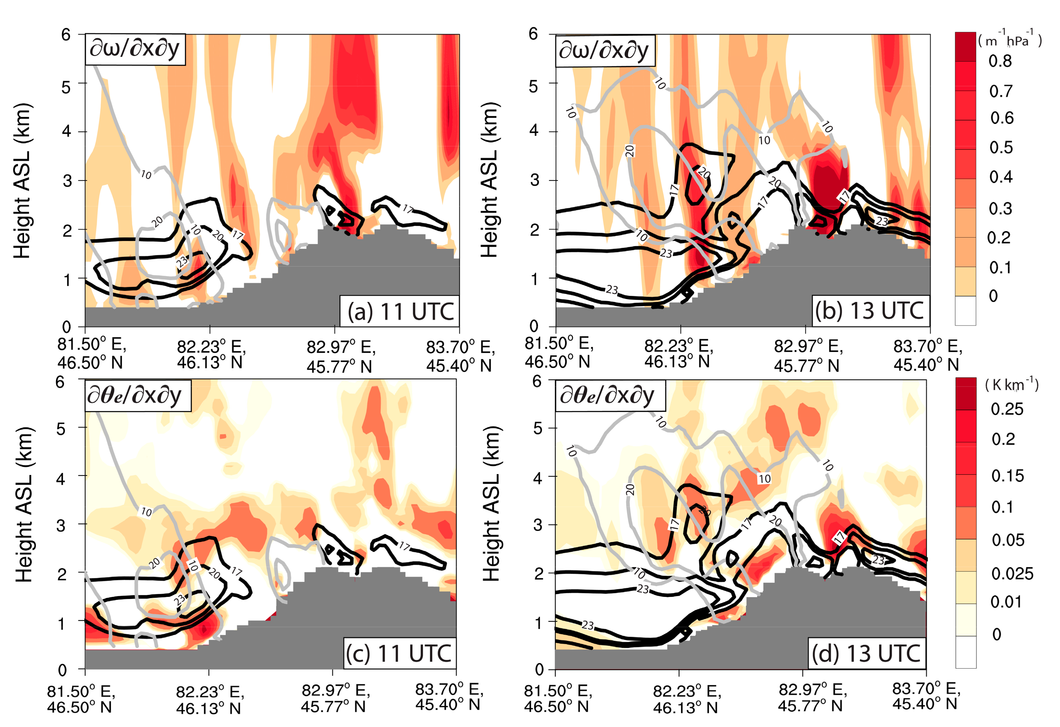
The distribution of the $\mathrm{HG}\omega$ at the early stage (Figure 13a) exhibited two high-value centers (shown by two blue dashed ellipses). One of them was located at the low level (<~2 km ASL) below S1, where it was collocated with the core region of the LLWJ. The other was in the intermediate area between S1 and S2 in the level of ~1.5–3.5 km ASL, where it was collocated with the area in front of the LLWJ exceeding the wind speed of 17 m s⁻¹. At the later stage (Figure 13b), there were three high-value centers of the $\mathrm{HG}\omega$ (indicated by three blue dashed ellipses) within the major part of the merged snowfall clouds. Their locations were also consistent with those of the high-value centers of F₄. These high-value centers were highly consistent with those of F₄ and implied a significant inhomogeneity of the momentum in the horizontal direction associated with the core region and leading edge of the LLWJ.

The $\mathrm{HG}{\theta }_e$ at the early stage (Figure 13c) showed a significantly high-value center at the low level below ~1.5 km ASL, which was located in front of the LLCF (indicated by the blue dashed ellipses). At the later stage (Figure 13d), with the further eastward movement of the LLCF, the high-value center of the $\mathrm{HG}{\theta }_e$ also moved over the windward slope (shown by the lower blue dashed ellipse). In addition, there were three other relatively weak high-value centers (denoted by the upper three blue dashed ellipses) in the merged snowfall cloud. The high value of the $\mathrm{HG}{\theta }_e$ at the low level indicated the baroclinicity of the lower troposphere due to the horizontal gradient of the temperature and moisture in front of the LLCF. The high value of the $\mathrm{HG}{\theta }_e$ within the merged snowfall cloud was probably due to the inhomogeneous release of latent heat in the clouds and (or) some dynamical processes such as gravity waves. The intensity of the $\mathrm{HG}\omega$ seemed to be generally higher than that of the $\mathrm{HG}{\theta }_e$ at the later stage; therefore, it can be deduced that the $\mathrm{HG}\omega$ contributed more than $\mathrm{HG}{\theta }_e$ In general, the baroclinicity of the lower troposphere due to the LLCF and the inhomogeneity of the momentum in the horizontal direction near the core region and leading edge of the LLWJ were jointly responsible for F₄.

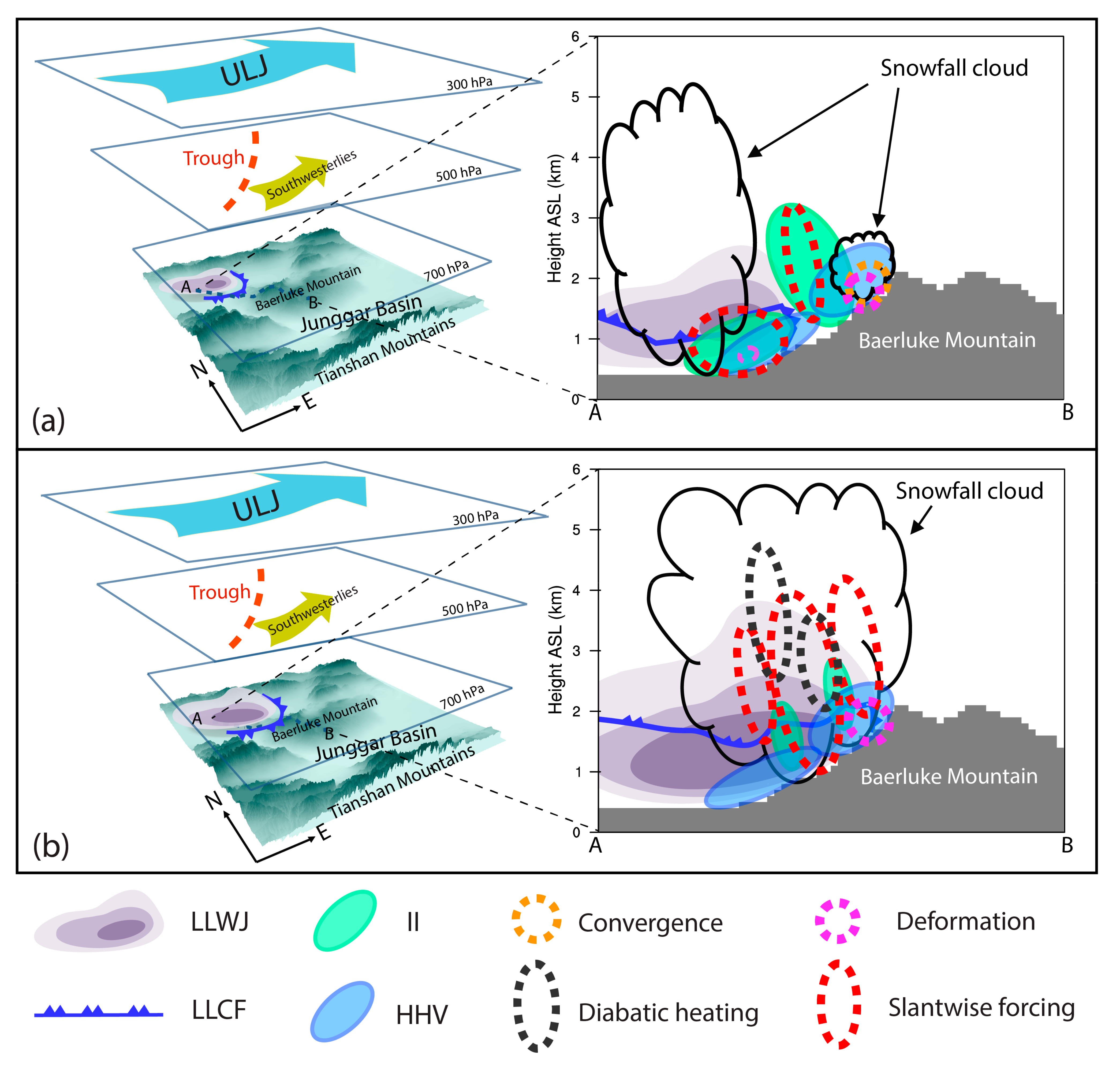
The tempo-spatial characteristics of these four components of the frontogenesis function can reveal the driving mechanisms for the release of the multiple instabilities that were crucial for the occurrence and development of the snowfall clouds analyzed above. These mechanisms are summarized in the conceptual model shown in Figure 14.

5. Summary and Discussion

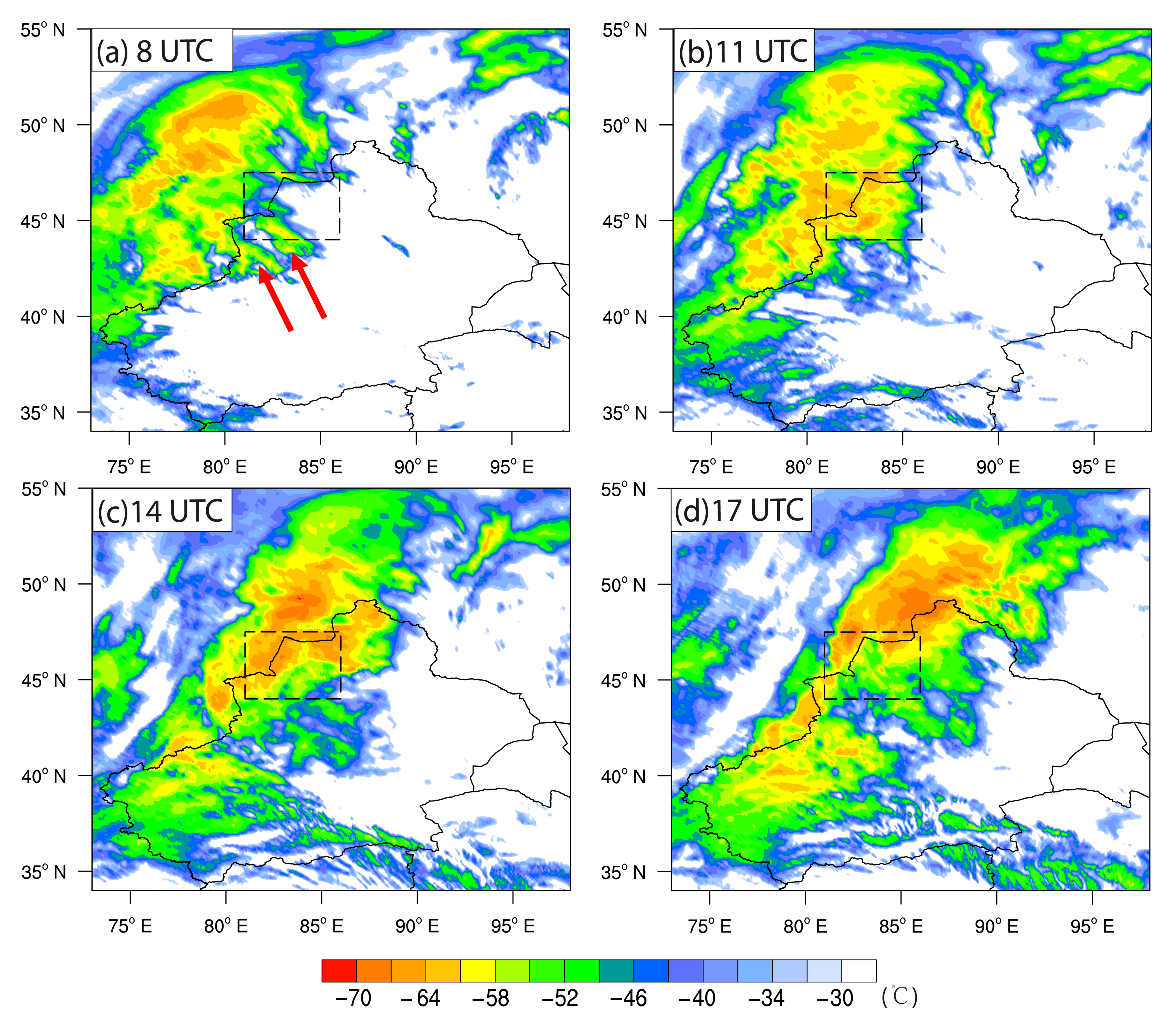
This paper investigated the mechanisms of the occurrence and development in the early period of a snowstorm associated with a low-level cold front (LLCF) and low-level westerly jet (LLWJ) in the western mountainous region of Junggar Basin, Xinjiang, Northwest China, on 22 January 2021. Tempo-spatial evaluation of the temperature of the black body (TBB) observed by the Fengyun-4A meteorological satellite (FY-4A) showed that the mesoscale clouds with TBB ≤ −64 °C during the heavy snowstorm lasted for about 6 h and caused continuous snowfall over the area around Baerluke Mountain, especially over its northwestern windward slope.

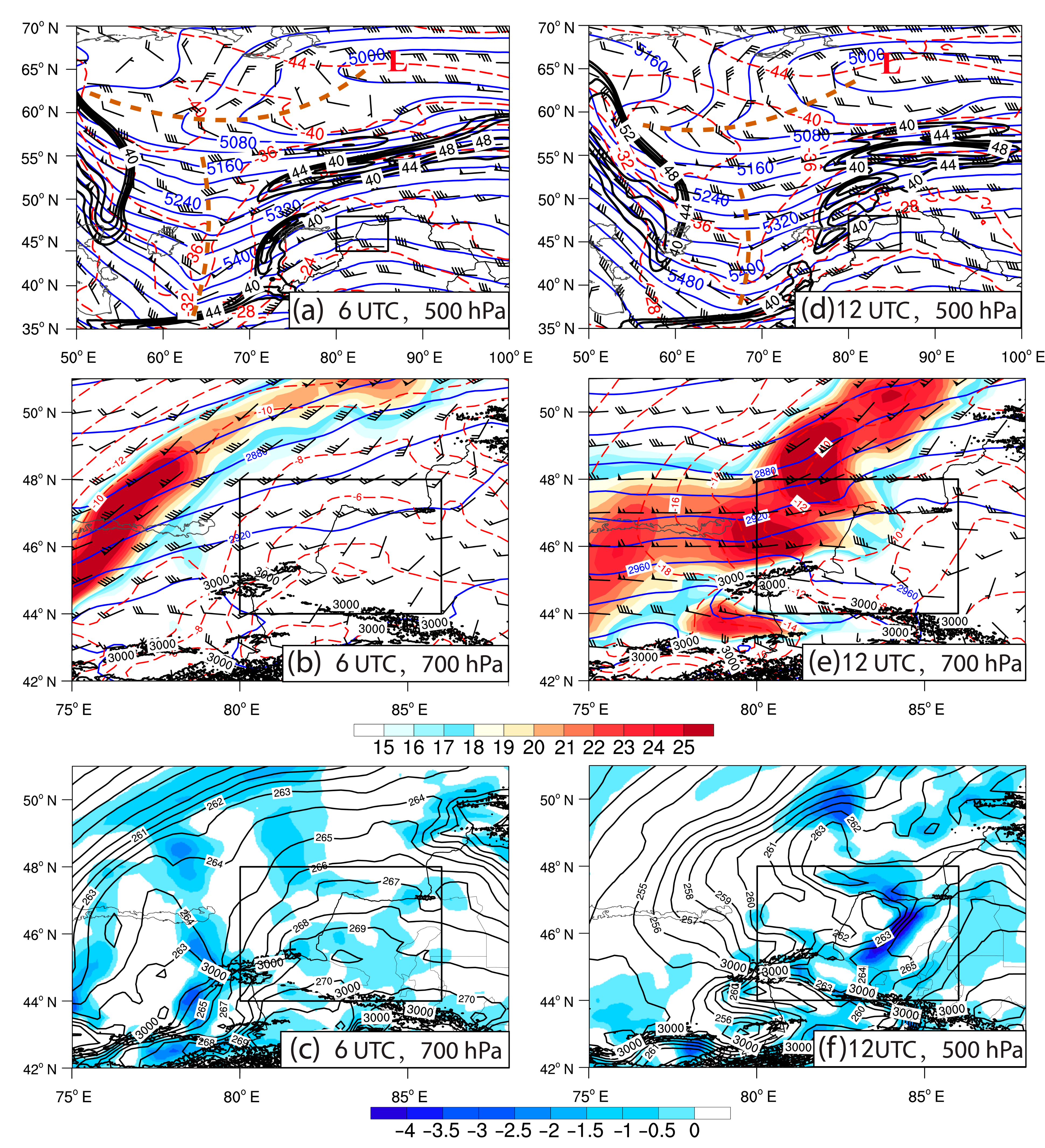
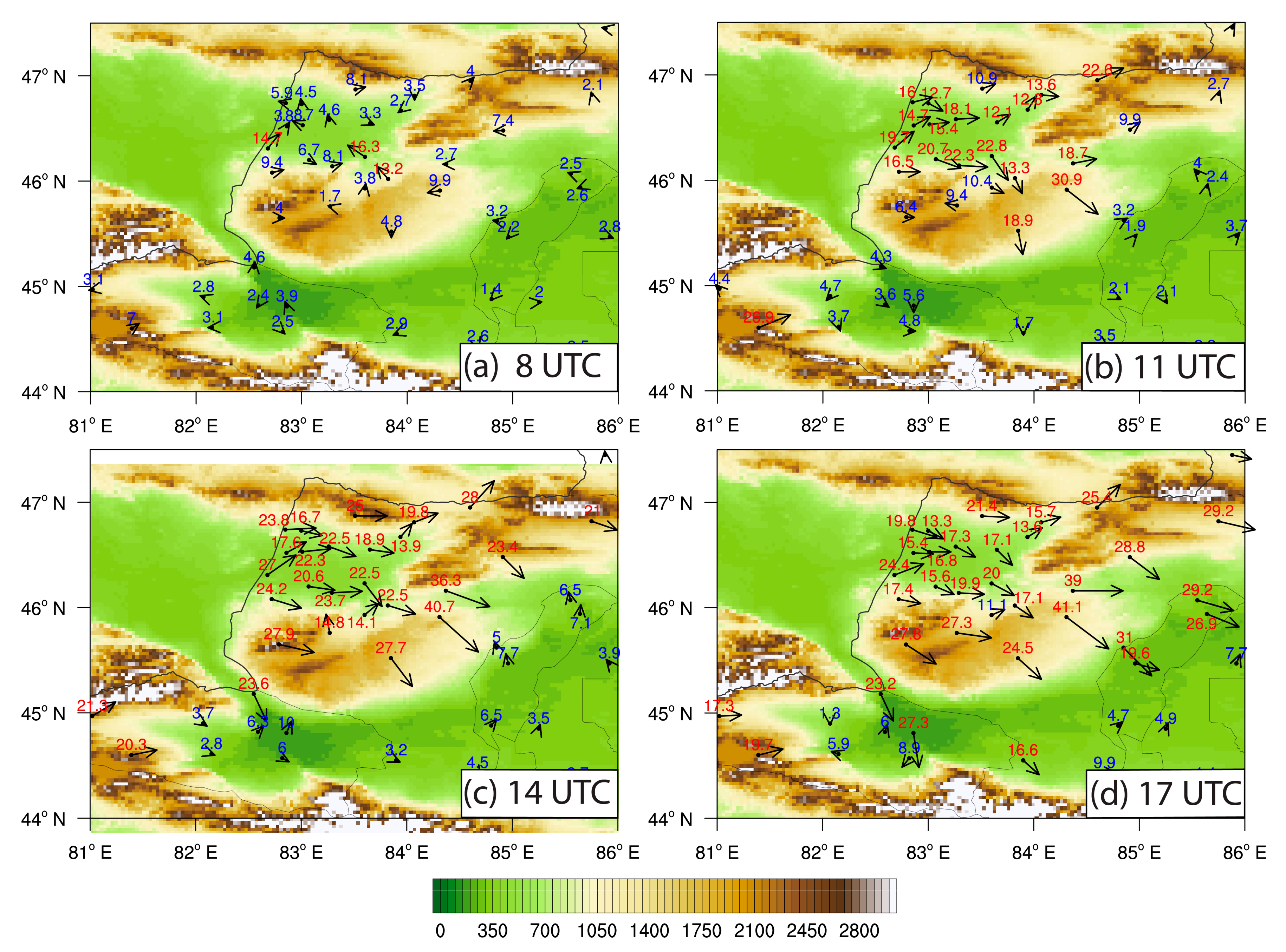
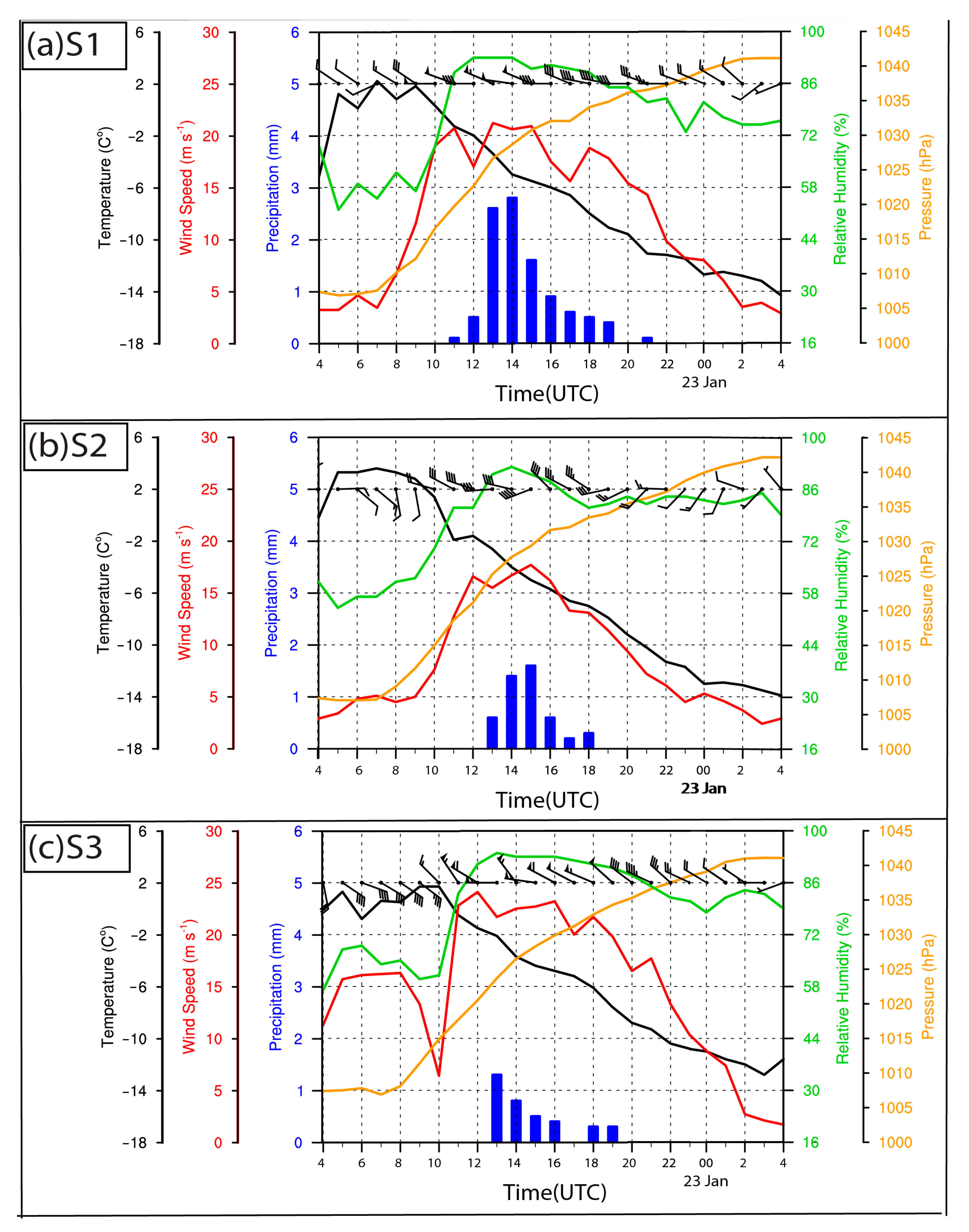
Basic meteorological elements observed by the surface-based automatic weather stations (AWSs) revealed that, before the occurrence of snowfall, there were abrupt changes in wind direction and a significant increase in wind speed (ranging from ~17 m s⁻¹ to ~24 m s⁻¹). Moreover, the three selected AWSs showed a significant increase in relative humidity (RH), monotonous temperature drop, and pressure jump. Consequently, it was concluded from the characteristics of these basic meteorological elements that the snowstorm was accompanied by an LLWJ and an LLCF delivering moist air. The snowstorm occurred under the synoptic background of an intense upper-level jet (ULJ) at 300 hPa and a short-wave trough at 500 hPa, along with an LLWJ and LLCF, which were also identified at 700 hPa. The study area was roughly located under the right side of the entrance region of the ULJ, indicating that an upper-level divergence occurred over the study area. Furthermore, the LLWJ and LLCF induced relatively intense advection of cold air and moisture to the study area, showing a relatively intense water vapor convergence near Baerluke Mountain. These synoptic and mesoscale conditions were quite favorable for the formation and development of the snowstorm.

This case was simulated using the Weather Research and Forecasting (WRF) model with a horizontal resolution of 3 km. The WRF simulation captured the overall patterns and features of the snowstorm event. The simulation results clearly exhibited the dynamic and thermodynamic features related to the LLWJ and LLCF, which were crucial for the formation and development of the snowstorm. In order to investigate the instability features related to the occurrence and development of the snowstorm, the moist potential vorticity (MPV) was calculated and analyzed over the major heavy precipitation area, which was roughly located near the northwestern windward slope of Baerluke Mountain.

It was found that, at the early stage of the occurrence and development of the snowfall clouds, relatively intense negative-MPV indicating the corresponding atmospheric instabilities were present below and near the major snowfall clouds and in the intermediate region between them. However, the extent and (or) intensity of the unstable layer below the snowstorm clouds decreased with the development of the snowstorm clouds at a later stage, denoting the release of the corresponding unstable energy. During the later stage, when the cloud system was maintained for about 3 h, the unstable layer below the clouds was also maintained for almost the same time.

In order to further investigate the specific instability characteristics, two components of the MPV were further analyzed. At the early stage (i.e., 11 UTC), the major instability over the plane region and windward slope was mainly dominated by the convective instability (CI) and inertial instability (II) (abbreviated as CI and II), whereas the hybrid effect of HGθe and VSHW (HHV) played important roles mainly at the lower level below ~1.5 km AGL over the upper part of the windward slope. At the later stage (i.e., 13 UTC), the overall intensity of the CI and II was released to some extent, and it disappeared over the plane region. However, it still made a major contribution at the mid-lower level (from ~1 km to 3~4 km ASL) within and (or) below the major part of the merged snowfall cloud. The HHV still contributed significantly at the low level below ~1.5 km AGL over the windward slope. During the later period, the CI and II had almost been released, and the snowfall clouds over the windward slope were supported merely by the HHV for several hours. Further studies on the specific factors influencing the CI and II and HHV showed that the CI and II were mainly dominated by the II that occurred in front and below the core region of the LLWJ. The HHV occurred at the low level below ~1 km AGL over the windward slope and was mainly attributable to the VSHW, whereas the $\mathrm{HG}{\theta }_e$ played a relatively weak positive role at the near-surface level below ~0.5 km AGL. The VSHW in the low layer was probably induced by the inhomogeneity of the momentum in the intermediate area between the LLWJ and windward slope topography. The atmospheric baroclinicity was reflected by the $\mathrm{HG}{\theta }_e$ probably due to the thermal inhomogeneity associated with LLCF.

Furthermore, the frontogenesis function was calculated and analyzed to further investigate the frontogenetical forcing mechanism required for the release of the above-mentioned instabilities. The results showed that, in general, the total frontogenesis was mainly dominated by the slantwise term during the whole period of occurrence and development of the snowfall clouds. In the early stage, except for the major dominant of the slantwise term, diabatic heating (probably due to the release of latent heat) also made a relatively weak positive contribution at the low level below the snowfall clouds. However, the convergence and deformation terms played a significant role at the lower level below ~0.4 km over the upper part of the windward slope. In the later stage, diabatic heating provided a relatively weak contribution at the mid-level (i.e., 2–5 km ASL) within the merged snowfall clouds, whereas the deformation made a significant contribution at the same low level below ~0.4 km over the upper part of the windward slope.

The physical meaning of the convergence and deformation terms indicates the local convergence and horizontal curvature due to the blocking effect and the special protruding shape of the windward slope of Baerluke Mountain, respectively. In addition, the slantwise term resulted from a combined effect of the baroclinicity of the lower troposphere due to the LLCF and the inhomogeneity of the momentum in a horizontal direction ($\mathrm{HG}\omega$) near the core region and ahead of the LLWJ. The contribution of the $\mathrm{HG}\omega$ seemed to be greater than that of the baroclinicity in the later stage.

A similar MPV-based diagnostic analysis of a snowstorm event that occurred in 2009 over the northern Tian Shan Mountains, Xinjiang, was conducted by Li et al. [42]. They pointed out that the increase in the absolute value of low-level MPV2 was one of the important causes of the snowstorm formation, which was consistent with our findings of the MPV2. However, our present study differs from their study in that the specific intuitional physical process that was mainly responsible for the occurrence of MPV2 and triggering mechanisms associated with an LLWJ and an LLCF were analyzed in detail based on frontogenesis function. Moreover, there were some other studies [26,34,41,54] that also examined the forcing mechanisms related to the release of instabilities according to the frontogenesis function during the occurrence and development of snowstorms, and none of them had further investigated the specific contributions of the several terms that made up the frontogenesis function. We found that there were some studies on summer precipitation in which they decomposed the frontogenesis function into several sum-terms and discussed their detailed contributions to the total frontogenesis. They stated that the convergence and deformation terms were the main contributors to the total frontogenesis function [35,36,37]. However, in the present paper, it was found that the slantwise term was the main contributor to total frontogenesis. Furthermore, we also further investigated the reason for the slantwise term and found that the contribution of the $\mathrm{HG}\omega$ resulting from the inhomogeneity of the momentum near the LLWJ would be greater than that of the baroclinicity due to the LLCF at the later stage of the snowstorm.

The conclusions of the main findings in the present study can be summarized as follows: The LLWJ along with the LLCF can provide not only significant contributions from an instability perspective but are also responsible for the frontogenetical forcing required for the release of instabilities during the occurrence and development of the snowstorm. In addition, it is believed that the findings regarding the specific contributions of the four terms of the frontogenetical forcing are also unique. Therefore, this work can be considered the first in-depth study that explains the mechanisms of a snowstorm associated with LLCF and LLWJ in the western mountainous region of the Junggar Basin, Xinjiang. However, additional simulations, including sensitivity experiments, will be conducted in the future to further clarify the orographic effect and microphysical processes that may be related to the occurrence and development of snowstorms in this region.

References

1. Burnett, A.W.; Kirby, M.E.; Mullins, H.T.; Patterson, W.P. Increasing Great Lake-effect snowfall during the twentieth century: A regional response to global warming? J. Clim. 2003, 16, 3535–3542. [Google Scholar] [CrossRef]
2. Changnon, S.A.; Changnon, D. A spatial and temporal analysis of damaging snowstorms in the United States. Nat. Hazards 2006, 37, 373–389. [Google Scholar] [CrossRef]
3. Chen, G.; Wang, W.-C.; Cheng, C.-T.; Hsu, H.-H. Extreme Snow Events along the Coast of the Northeast United States: Potential Changes due to Global Warming. J. Clim. 2021, 34, 2337–2353. [Google Scholar] [CrossRef]
4. Chen, Z.; Xu, Y.; Zhou, X.; Tang, J.; Kuzyakov, Y.; Yu, H.; Fan, J.; Ding, W. Extreme rainfall and snowfall alter responses of soil respiration to nitrogen fertilization: A 3-year field experiment. Glob. Chang. Biol. 2017, 23, 3403–3417. [Google Scholar] [CrossRef] [PubMed]
5. Li, R.; Tang, Y.; Rouzi, A. Atmospheric Circulation and Water Vapor Characteristics of Snowstorm Anomalies in Northern Xinjiang in 2010. Plateau Meteorol. 2015, 34, 155–162. [Google Scholar] [CrossRef]
6. Li, Y.; Niu, S.; Lv, J.; Wang, J.; Wsng, T.; Husng, Q.; Wsng, Y. Analysis on Microphysical Characteristics of Three Blizzard Processes in Nanjing in the Winter of 2018. Chin. J. Atmos. Sci. 2019, 43, 1095–1108. [Google Scholar] [CrossRef]
7. Zhou, B.; Wang, Z.; Shi, Y. Possible Role of Hadley Circulation Strengthening in Interdecadal Intensification of Snowfalls Over Northeastern China Under Climate Change. J. Geophys. Res.-Atmos. 2017, 122, 11638–11650. [Google Scholar] [CrossRef]
8. Smart, D.; Browning, K. An under-forecast snowstorm associated with a small but deep tropopause depression. Weather 2020, 75, 372–377. [Google Scholar] [CrossRef]
9. Campbell, L.S.; Steenburgh, W.J.; Yamada, Y.; Kawashima, M.; Fujiyoshi, Y. Influences of Orography and Coastal Geometry on a Transverse-Mode Sea-Effect Snowstorm over Hokkaido Island, Japan. Mon. Weather Rev. 2018, 146, 2201–2220. [Google Scholar] [CrossRef]
10. Kristovich, D.A.R.; Bard, L.; Stoecker, L.; Geerts, B. Influence of Lake Erie on a Lake Ontario Lake-Effect Snowstorm. J. Appl. Meteorol. Climatol. 2018, 57, 2019–2033. [Google Scholar] [CrossRef]
11. Wang, L.; Fan, K. Synoptic and Climatic Conditions of an Extreme Snowstorm Event Over Northeast China and Its Climate Predictability. Front. Earth Sci. 2022, 10, 5061. [Google Scholar] [CrossRef]
12. Ellis, A.W.; Johnson, J.J. Hydroclimatic analysis of snowfall trends associated with the North American Great Lakes. J. Hydrometeorol. 2004, 5, 471–486. [Google Scholar] [CrossRef]
13. Kawase, H.; Hara, M.; Yoshikane, T.; Ishizaki, N.N.; Uno, F.; Hatsushika, H.; Kimura, F. Altitude dependency of future snow cover changes over Central Japan evaluated by a regional climate model. J. Geophys. Res.-Atmos. 2013, 118, 12444–12457. [Google Scholar] [CrossRef]
14. Notaro, M.; Bennington, V.; Vavrus, S. Dynamically Downscaled Projections of Lake-Effect Snow in the Great Lakes Basin. J. Clim. 2015, 28, 1661–1684. [Google Scholar] [CrossRef]
15. Sun, B.; Wang, H.J.; Wu, B.W.; Xu, M.; Zhou, B.T.; Li, H.X.; Wang, T. Dynamic Control of the Dominant Modes of Interannual Variability of Snowfall Frequency in China. J. Clim. 2021, 34, 2777–2790. [Google Scholar] [CrossRef]
16. Sun, B.; Wang, H.J.; Zhou, B.T. Climatic Condition and Synoptic Regimes of Two Intense Snowfall Events in Eastern China and Implications for Climate Variability. J. Geophys. Res.-Atmos. 2019, 124, 926–941. [Google Scholar] [CrossRef]
17. Zhou, B.T.; Wang, Z.Y.; Sun, B.; Hao, X. Decadal Change of Heavy Snowfall over Northern China in the Mid-1990s and Associated Background Circulations. J. Clim. 2021, 34, 825–837. [Google Scholar] [CrossRef]
18. Wang, Z.Y.; Zhou, B.T. Large-scale atmospheric circulations and water vapor transport influencing inter interannual variations of intense snowfalls in northern China. Chin. J. Geophys. 2018, 61, 2654–2666. [Google Scholar] [CrossRef]
19. Alcott, T.I.; Steenburgh, W.J. Orographic Influences on a Great Salt Lake-Effect Snowstorm. Mon. Weather Rev. 2013, 141, 2432–2450. [Google Scholar] [CrossRef]
20. Campbell, L.S.; Steenburgh, W.J. The OWLeS IOP2b lake-effect snowstorm: Mechanisms contributing to the Tug Hill precipitation maximum. Mon. Weather Rev. 2017, 145, 2461–2478. [Google Scholar] [CrossRef]
21. Lang, C.E.; McDonald, J.M.; Gaudet, L.; Doeblin, D.; Jones, E.A.; Laird, N.F. The Influence of a Lake-to-Lake Connection from Lake Huron on the Lake-Effect Snowfall in the Vicinity of Lake Ontario. J. Appl. Meteorol. Climatol. 2018, 57, 1423–1439. [Google Scholar] [CrossRef]
22. Umek, L.; Gohm, A. Lake and Orographic Effects on a Snowstorm at Lake Constance. Mon. Weather Rev. 2016, 144, 4687–4707. [Google Scholar] [CrossRef]
23. Aikins, J.; Friedrich, K.; Geerts, B.; Pokharel, B. Role of a Cross-Barrier Jet and Turbulence on Winter Orographic Snowfall. Mon. Weather Rev. 2016, 144, 3277–3300. [Google Scholar] [CrossRef]
24. Ma, S.; Ran, L.; Cao, J. Diagnosis and Analysis of Vertical Motion during Complex Topographical Heavy Snowfall. Chin. J. Atmos. Sci. 2021, 45, 1127–1145. [Google Scholar] [CrossRef]
25. Gehring, J.; Vignon, E.; Billault-Roux, A.-C.; Ferrone, A.; Protat, A.; Alexander, S.P.; Berne, A. Orographic Flow Influence on Precipitation During an Atmospheric River Event at Davis, Antarctica. J. Geophys. Res.-Atmos. 2022, 127, e2021JD035210. [Google Scholar] [CrossRef]
26. Schumacher, R.S.; Schultz, D.M.; Knox, J.A. Convective Snowbands Downstream of the Rocky Mountains in an Environment with Conditional, Dry Symmetric, and Inertial Instabilities. Mon. Weather Rev. 2010, 138, 4416–4438. [Google Scholar] [CrossRef]
27. Zhao, Y.; Fu, L.; Yang, C.F.; Chen, X.F. Case Study of a Heavy Snowstorm Associated with an Extratropical Cyclone Featuring a Back-Bent Warm Front Structure. Atmosphere 2020, 11, 1272. [Google Scholar] [CrossRef]
28. Yu, B.; Hong, Y.; Zhang, Y.; Tulinisha; Xu, T.; Li, N. Multiscale Configuration and Mechanism Analysis of an Extreme Snowstorm on the Two Sides of Tianshan Mountains. Desert Oasis Meteorol. 2020, 14, 11–18. [Google Scholar] [CrossRef]
29. Sanders, F.; Bosart, L.F. Mesoscale structure in the megalopolitan snowstorm of 11–12 February 1983. Part I: Frontogenetical forcing and symmetric instability. J. Atmos. Sci. 1985, 42, 1050–1061. [Google Scholar] [CrossRef]
30. Wang, J.; Ding, Y. Research of Moist Symmetric Instability in a Strong Snowfall in North China. Acta Meteorol. Sin. 1995, 4, 451–460. [Google Scholar]
31. Schultz, D.M.; Schumacher, P.N. The use and misuse of conditional symmetric instability. Mon. Weather Rev. 1999, 127, 2709–2732, Erratum in Mon. Weather Rev. 2000, 128, 1573–1573. [Google Scholar] [CrossRef]
32. Schumacher, R.S.; Schultz, D.M.; Knox, J.A. Influence of Terrain Resolution on Banded Convection in the Lee of the Rocky Mountains. Mon. Weather Rev. 2015, 143, 1399–1416. [Google Scholar] [CrossRef]
33. Taylor, S.M.; Kaplan, M.L.; Lin, Y.-L. Multiscale Dynamics of the February 11–12, 2010, Deep South US Snowstorm Event. Adv. Meteorol. 2017, 2017, 6301026. [Google Scholar] [CrossRef]
34. Li, N.; Jiao, B.; Ran, L.; Shen, X.; Qi, Y. On the Mechanism of a Terrain-Influenced Snow Burst Event during Midwinter in Northeast China. Adv. Atmos. Sci. 2021, 38, 800–816. [Google Scholar] [CrossRef]
35. Duan, X.; Duan, W.; Zhang, Y.; Wang, M. Diagnostic analysis of frontogenesis and frontolysis of Kunming quasi-stationary front in early 2008 based on frontogenesis function. Chin. J. Atmos. Sci. 2019, 43, 325–338. [Google Scholar] [CrossRef]
36. Xu, Y.; Wu, S.; Yang, W.; Liu, X.; Huang, Y. Analysis of Frontogenesis and Circulation Characteristics of the Meiyu Front with Heavy Precipitation in Zhejiang Province. Chin. J. Atmos. Sci. 2019, 43, 1219–1232. [Google Scholar] [CrossRef]
37. He, Z.; Zhu, L.; Zhang, X.; Wang, L.; Wu, L.; Xi, L. Diagnosis of the Frontgenesis and Instabilities in Two Continuous Autumn Torrential Rain Days in Henan Province. Meteorol. Mon. 2022, 48, 1101–1115. [Google Scholar] [CrossRef]
38. Huang, M.; Cao, Z.; Shen, X. A Study on the Relationship between Conditional Symmetric Instability and Northward Jumping of the Summer Monsoon Rainband in East China. Chin. J. Atmos. Sci. 2019, 43, 943–958. [Google Scholar] [CrossRef]
39. Huang, X.; Zhou, Y.; Ran, L.; KALIM, U.; Zeng, Y. Analysis of the Environmental Field and Unstable Conditionson a Rainstorm Event in the Ili Valley of Xinjiang. Chin. J. Atmos. Sci. 2021, 45, 148–164. [Google Scholar] [CrossRef]
40. Li, J.; Pan, X.; Zang, Z.; Zhao, D.; Ming, S. Diagnostic analysis of moist potential vorticity for a rainstorm in North China. Torrential. Rain Disasters 2016, 35, 158–165. [Google Scholar]
41. Feng, L.; Song, P.; Zheng, F.; He, Z. Diagnostic Analysis of a Severe Regional Snowstorm Event in the Early Winter of 2016 in Henan Province, China. Chin. J. Atmos. Sci. 2020, 44, 13–26. [Google Scholar] [CrossRef]
42. Li, R.; Tang, Z.; Lu, G. Moist Potential Vorticity of the northern Xinjiang blizzard process. Desert Oasis Meteorol. 2013, 7, 1–6. [Google Scholar] [CrossRef]
43. Zhang, G.; Yao, X.; Sun, Y.; Meng, X.; Zhong, X.; Liu, W. Diagnostic Analysis of a Snowstrom in Daxinganling Region. Meteorol. Sci. Technol. 2018, 46, 971–978. [Google Scholar] [CrossRef]
44. Abulikemu, A.; Ming, J.; Xu, X.; Zhuge, X.Y.; Wang, Y.; Zhang, Y.H.; Zhang, S.S.; Yu, B.X.; Aireti, M. Mechanisms of Convection Initiation in the Southwestern Xinjiang, Northwest China: A Case Study. Atmosphere 2020, 11, 1335. [Google Scholar] [CrossRef]
45. Abulikemu, A.; Wang, Y.; Gao, R.X.; Wang, Y.; Xu, X. A Numerical Study of Convection Initiation Associated with a Gust Front in Bohai Bay Region, North China. J. Geophys. Res.-Atmos. 2019, 124, 13843–13860. [Google Scholar] [CrossRef]
46. Abulikemu, A.; Xu, X.; Wang, Y.; Ding, J.F.; Zhang, S.S.; Shen, W.Q. A modeling study of convection initiation prior to the merger of a sea-breeze front and a gust front. Atmos. Res. 2016, 182, 10–19. [Google Scholar] [CrossRef]
47. Kong, M.N.; Abulikemu, A.; Zheng, J.J.; Aireti, M.; An, D.W. A Case Study on Convection Initiation Associated with Horizontal Convective Rolls over Ili River Valley in Xinjiang, Northwest China. Water 2022, 14, 1017. [Google Scholar] [CrossRef]
48. Skamarock, C.; Klemp, B.; Dudhia, J.; Gill, O.; Liu, Z.; Berner, J.; Wang, W.; Powers, G.; Duda, G.; Barker, D.; et al. A Description of the Advanced Research WRF Model Version 4 (No. NCAR/TN-556+STR). Natl. Cent. Atmos. Res. 2019, 145, 145. [Google Scholar] [CrossRef]
49. Hong, S.-Y.; Noh, Y.; Dudhia, J. A new vertical diffusion package with an explicit treatment of entrainment processes. Mon. Weather Rev. 2006, 134, 2318–2341. [Google Scholar] [CrossRef]
50. Jimenez, P.A.; Dudhia, J.; Gonzalez-Rouco, J.F.; Navarro, J.; Montavez, J.P.; Garcia-Bustamante, E. A Revised Scheme for the WRF Surface Layer Formulation. Mon. Weather Rev. 2012, 140, 898–918. [Google Scholar] [CrossRef]
51. Chen, F.; Dudhia, J. Coupling an advanced land surface-hydrology model with the Penn State-NCAR MM5 modeling system. Part II: Preliminary model validation. Mon. Weather Rev. 2001, 129, 587–604. [Google Scholar] [CrossRef]
52. Iacono, M.J.; Delamere, J.S.; Mlawer, E.J.; Shephard, M.W.; Clough, S.A.; Collins, W.D. Radiative forcing by long-lived greenhouse gases: Calculations with the AER radiative transfer models. J. Geophys. Res.-Atmos. 2008, 113, D13. [Google Scholar] [CrossRef]
53. Kain, J.S. The Kain-Fritsch convective parameterization: An update. J. Appl. Meteorol. 2004, 43, 170–181. [Google Scholar] [CrossRef]
54. Li, N.; Jiao, B.; Ran, L.; Gao, Z.; Gao, S. Influence of the Upstream Terrain on the Formation of a Cold Frontal Snowband in Northeast China. Asia-Pac. J. Atmos. Sci. 2022, 58, 243–264. [Google Scholar] [CrossRef]
55. Luhunga, P.M.; Djolov, G. Evaluation of the Use of Moist Potential Vorticity and Moist Potential Vorticity Vector in Describing Annual Cycles of Rainfall over Different Regions in Tanzania. Front. Earth Sci. 2017, 5, 7. [Google Scholar] [CrossRef]
56. Gao, S.; Wang, X.; Zhou, Y. Generation of generalized moist potential vorticity in a frictionless and moist adiabatic flow. Geophys. Res. Lett. 2004, 31, L12113. [Google Scholar] [CrossRef]
57. Gao, S.T.; Zhou, F.-F. Water vapour potential vorticity and its applications in tropical cyclones. Chin. Phys. Lett. 2008, 25, 3830–3833. [Google Scholar]
58. Yao, X.; Gao, Y.; Ma, J. MPV-Q* view of vorticity development in a saturated atmosphere. Atmos. Res. 2020, 244, 105058. [Google Scholar] [CrossRef]
59. Bennetts, D.A.; Hoskins, B.J. Conditional symmetric instability—A possible explanation for frontal rainbands. Q. J. R. Meteorol. Soc. 1979, 105, 945–962. [Google Scholar] [CrossRef]
60. Marquet, P. On the definition of a moist-air potential vorticity. Q. J. R. Meteorol. Soc. 2014, 140, 917–929. [Google Scholar] [CrossRef]
61. Wu, G.; Cai, Y.; Tang, X. Moist Potential Vorticity and Slantwise Vorticity Development. Acta Meteorol. Sin. 1995, 53, 387–405. [Google Scholar]
62. Liu, J.; Zhou, Y.; Yang, L.; Zeng, Y.; Liu, W. The Instability and its Trigger Mechanism of Extreme Precipitation Event in the Yili River Valley on 31 July 2016. Chin. J. Atmos. Sci. 2019, 43, 1204–1218. [Google Scholar] [CrossRef]
63. Ninomiya, K. Characteristics of Baiu front as a predominant subtropical front in the summer Northern Hemisphere. J. Meteorol. Soc. Jpn. 1984, 62, 880–894. [Google Scholar] [CrossRef]
64. Ninomiya, K. Large-and meso-α-scale characteristics of Meiyu/Baiu front associated with intense rainfalls in 1–10 July 1991. J. Meteorol. Soc. Jpn. 2000, 78, 141–157. [Google Scholar] [CrossRef]
65. Yang, S.; Gao, S.; Lu, C. Investigation of the mei-yu front using a new deformation frontogenesis function. Adv. Atmos. Sci. 2015, 32, 635–647. [Google Scholar] [CrossRef]
Figure 1. (a) Geographic location and terrain altitude (shading, unit: m) of the study area where the snowstorm occurred. The black five-pointed star (☆) indicates the location (46.73° N, 83° E) of the Tacheng Radiosonde station, and the red dots indicate the locations of the ground-based automatic weather stations (AWSs) (S1, S2, and S3). The solid black and thin gray lines indicate the national and district boundaries, respectively. (b) Geographic locations and terrain altitudes (shading, unit: m) of the WRF model domains.
Atmosphere 14 00919 g001
Figure 2. (ad) Geopotential height (blue solid lines, units: gpm), temperature (red dashed lines, units: °C), and wind fields (half barbs, full barbs, and flags represent 2, 4, and 20 m s−1, respectively) on 22 January 2021 derived from ERA5 data. The overlaid black contours (unit: m s−1) in (a) and (b) indicate that the upper-level jet exceeded 40 m s−1 at 300 hPa, the thick brown dashed line indicates the trough, and the letter “L” indicates the low-pressure center. The shaded colored areas in (c) and (d) indicate that the lower-level jet (unit: m s−1) exceeded 15 m s−1, and the overlaid black contours indicate topography over 3000 m above sea level (ASL). (e,f) Water vapor flux divergence (shading, unit: g hPa−1 cm2 s−1) and potential temperature (black contours, unit: K). The specific time and isobaric surface level are shown in the lower right corner of each panel, and the rectangular area in each panel denotes the study area shown in Figure 1a.
Atmosphere 14 00919 g002
Figure 3. (ad) Temperature of the black body (TBB, shading, unit: °C) over the top of the snowfall cloud observed by the FY-4A meteorological satellite on 22 January 2021. The black dashed rectangular area denotes the study area, as shown in Figure 1a. The specific time is shown in the upper left corner of each panel. Two red arrows in (a) represent the position of meso-β scale banded clouds.
Atmosphere 14 00919 g003
Figure 4. (ad) Terrain altitude (shading, unit: m) and hourly maximum wind (black vector arrows) observed by the ground-based automatic weather stations (AWSs). The values of hourly maximum wind speed observed by AWSs are shown for each station, and the values over and under 12 m s−1 are indicated with numbers in red and blue, respectively. The specific time is shown in the upper left corner of each panel.
Atmosphere 14 00919 g004
Figure 5. Evolution of precipitation (blue bars, unit: mm), temperature (black lines, units: °C), relative humidity (green lines, unit: %), pressure (pale brown lines, unit: hPa), and wind information (wind barbs, half barbs, full barbs, and flags represent 2, 4, and 20 m s−1, respectively; red lines show the wind speed, units: m s−1) observed by ground-based automatic weather stations (a) S1, (b) S2, and (c) S3, respectively, (see the locations of S1, S2, and S3 in Figure 1a) from 4 UTC on 22 January to 4 UTC on 23 January 2021.
Atmosphere 14 00919 g005
Figure 6. (a) Observed 24 h accumulated precipitation (colorful symbols, units: mm) observed by the ground-based automatic weather stations from 12 UTC on 22 January to 12 UTC on 23 January 2021. (b) Simulated 24 h accumulated precipitation (shading, units: mm) during the same time as (a).
Atmosphere 14 00919 g006
Figure 7. (a) Skew T-logP diagram derived from an observed balloon sounding at Tacheng weather station (marked with symbol “☆” in Figure 1a) at 12 UTC on 22 January 2021. (b) is the same as (a) but derived from the WRF simulation data at the same time and the same location.
Atmosphere 14 00919 g007
Figure 8. (ad) Simulated composed radar reflectivity (shading, units: dBZ), the height of topography (black solid contours, unit: m), and wind field (half barbs, full barbs, and flags represent 2, 4, and 20 m s−1, respectively) at 1000 m ASL on 22 January 2021. The red line segment AB indicates the location of the vertical cross-section which is shown in Figure 9, Figure 10, Figure 11, Figure 12 and Figure 13. The specific time is shown in the lower right corner of each panel. (e) Simulated 24 h accumulated precipitation (blue contour, units: mm) from 6 UTC on 22 January to 6 UTC on 23 January 2021 along the line segment AB, and the gray shading indicates the topography.
Atmosphere 14 00919 g008
Figure 9. (ad) Vertical cross-section of the composed reflectivity (shading, units: dBZ) and potential temperature (gray contours, units: K) along the line AB (shown in Figure 8) at 10, 11, 12, and 13 UTC on 22 January 2021. The red dashed lines indicate the LLCF and the hollow red arrows indicate the location of the leading edge of the LLCF on the ground. The two black dashed lines indicate the boundaries on both sides of the fronts formed at the top of the mountain, and the two filled red arrows indicate the positions of these two fronts. (eh) are the same as (ad), except for the potential temperature (θ, shading, units: K), composed reflectivity (black solid contours, units: dBZ), and horizontal wind speed (black vector arrows). (il) are the same as (ad), except for the horizontal wind speed (shading, units: m s−1). The gray shading indicates the topography, and the specific time is shown in the lower right corner of each panel.
Atmosphere 14 00919 g009
Figure 10. (ac) Vertical cross-section of the moist potential vorticity (MPV, shading, units: PVU, 1 PVU = 10−6 m2 K s−1 kg−1) and composed reflectivity (black solid contours, units: dBZ) along the line AB at 11, 13, and 15 UTC on 22 January 2021, respectively. (df) are the same as (ac), except for the MPV1, and (gi) are the same as (ac), except for the MPV2. The green dashed lines indicate the LLCF, the gray shading indicates the topography, and the specific time is shown in the lower right corner of each panel.
Atmosphere 14 00919 g010
Figure 11. (a) Vertical cross-section of the MPV1 (shading, units: PVU, 1 PVU = 10−6 m2 K s−1 kg−1) and horizontal wind speed (dark green contours, units: m s−1) along the line AB at 11 UTC on 22 January 2021. (b,c) are the same as (a), except for the inertial instability (II, shading, units:10−4 s−1) and convective instability (CI, shading, units: K km−1), respectively. (df) are the same as (a), except for the MPV2 (shading, units: PVU, 1 PVU = 10−6 m2 K s−1 kg−1), vertical shear of the horizontal wind (i.e., VSHW, shading, units: 10−3 m s−1 hPa−1), and horizontal gradient of the equivalent potential temperature (i.e., HG θ e , shading, units: K km−1) at 15 UTC on 22 January 2021. The red dashed lines indicate the LLCF, the gray shading indicates the topography, and the specific time is shown in the lower right corner of each panel.
Atmosphere 14 00919 g011
Figure 12. (a) Vertical cross-section of the total frontogenesis (Ft) (shading, units: 10−8 K m−1 s−1) and composed reflectivity (black solid contours, units: dBZ) along the line AB (shown in Figure 8) at 11 UTC on 22 January 2021. (be) are the same as (a), except for the four components of the Ft (F1, F2, F3, and F4, respectively). The red dashed line denotes the cold front within the boundary layer westerly jet (BLWJ), and the hollow red arrow indicates the location of the leading edge of the cold front on the ground. (fj) are the same as (ae), except for the time at 15 UTC. The gray shading indicates the topography, and the specific time is shown in the lower right corner of each panel.
Atmosphere 14 00919 g012
Figure 13. (a,b) Vertical cross-section of the horizontal gradient of vertical velocity (i.e., HG ω shading, units:10−3 Pa s−1 m−1), horizontal wind speed (bold black contours, units: m s−1), and composed reflectivity (gray contours, units: dBZ). (c,d) are the same as (a,b), except for the horizontal gradient of equivalent potential temperature (i.e., HG θ e , shading, units: K km−1). The gray shading indicates the topography, and the specific time is shown in the lower right corner of each panel.
Atmosphere 14 00919 g013
Figure 14. Schematic model summarizing the mechanism of the occurrence and development of the snowstorm event investigated in the present study. (a) Early Stage, (b) Later Stage.
Atmosphere 14 00919 g014