

Estimation of Carbonaceous Aerosol Sources under Extremely Cold Weather Conditions in an Urban Environment

 , , ,
, , ,
Abstract
:1. Introduction
2. Materials and Methods
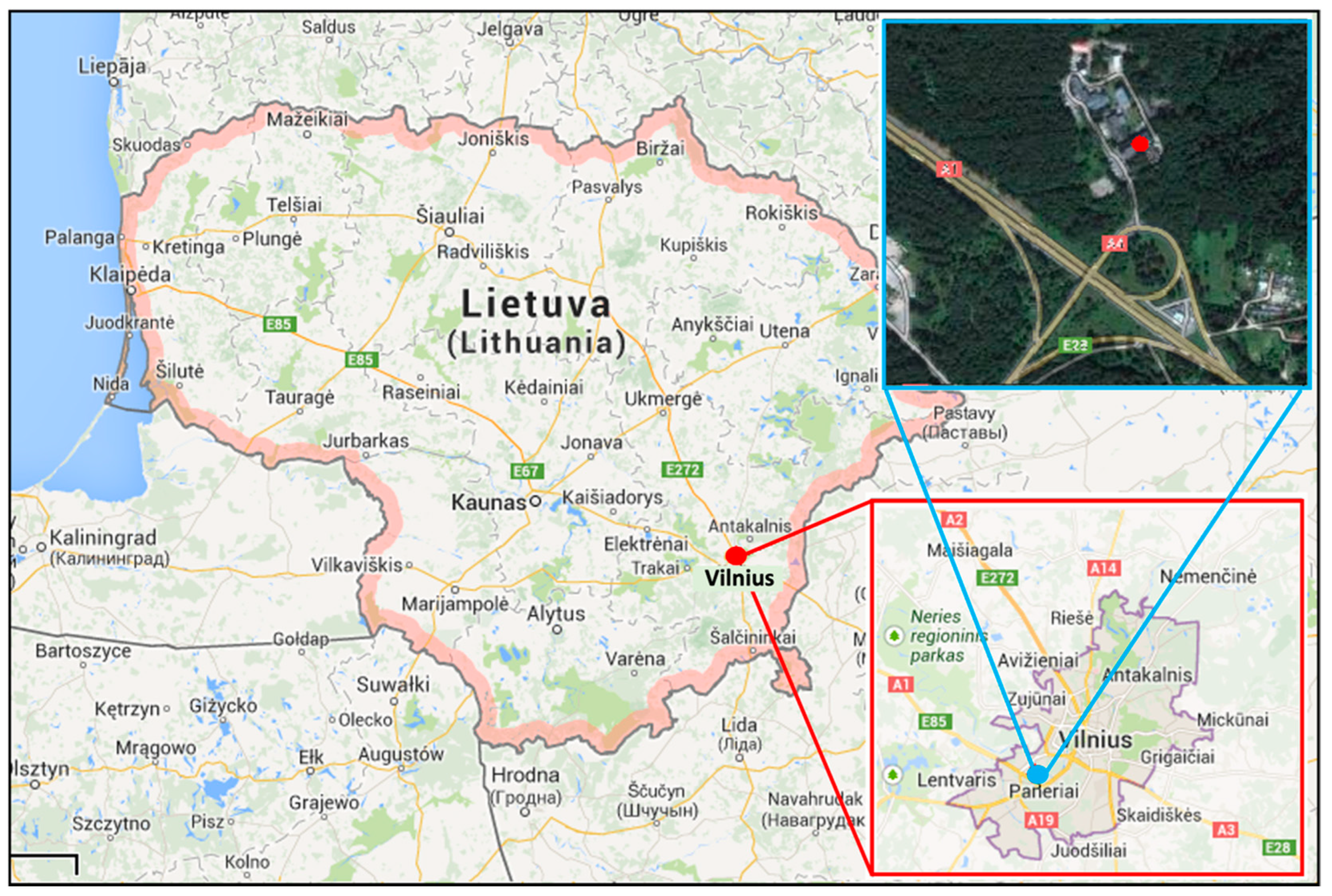
2.1. Site Description
2.2. Instrumentation
2.2.1. Organic Aerosol
2.2.2. Black Carbon
2.3. Source Apportionment Techniques
2.3.1. Organic Aerosol Source Apportionment
2.3.2. Black Carbon Source Apportionment
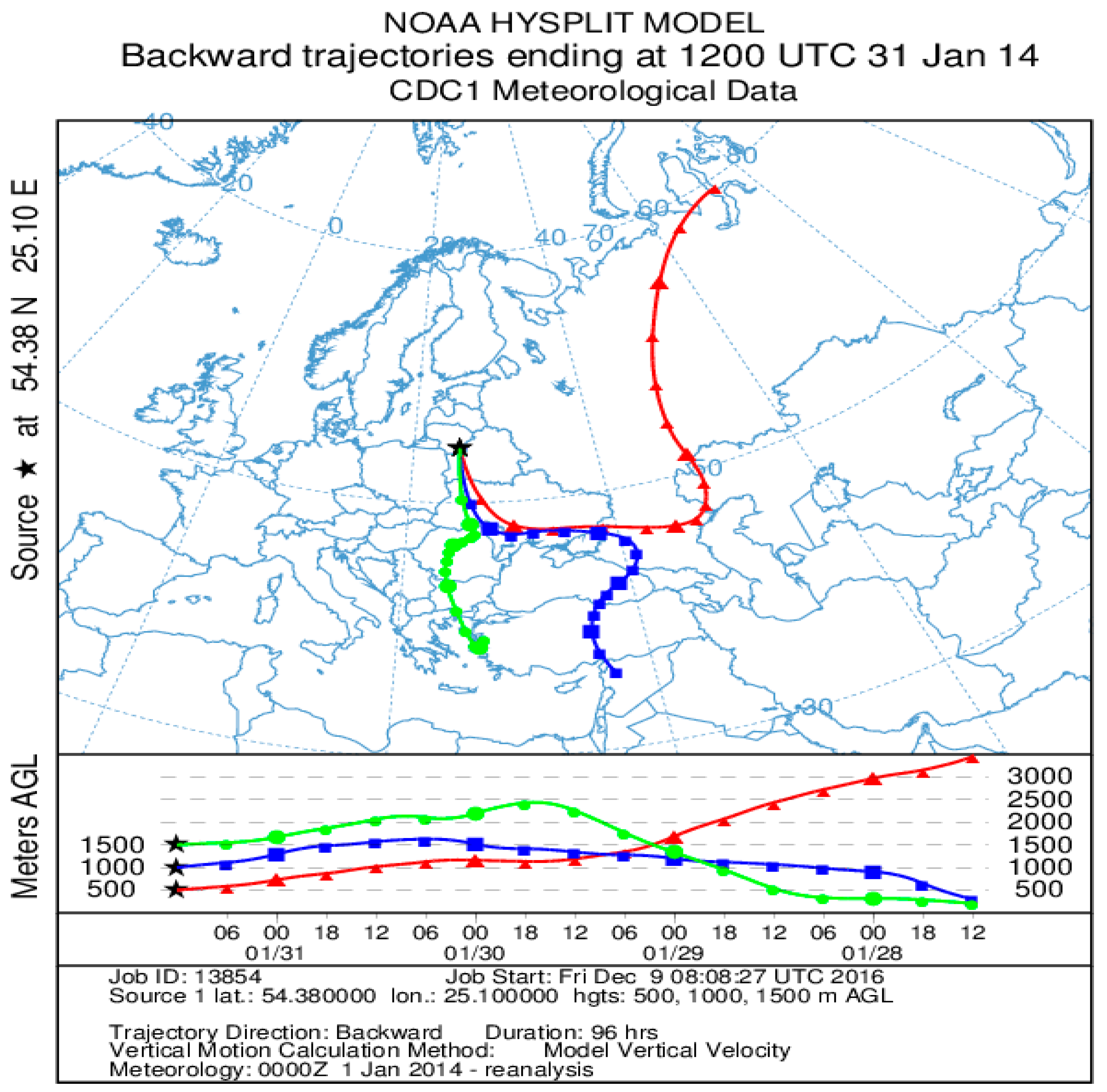
2.4. Air Mass Backward Trajectories
3. Results
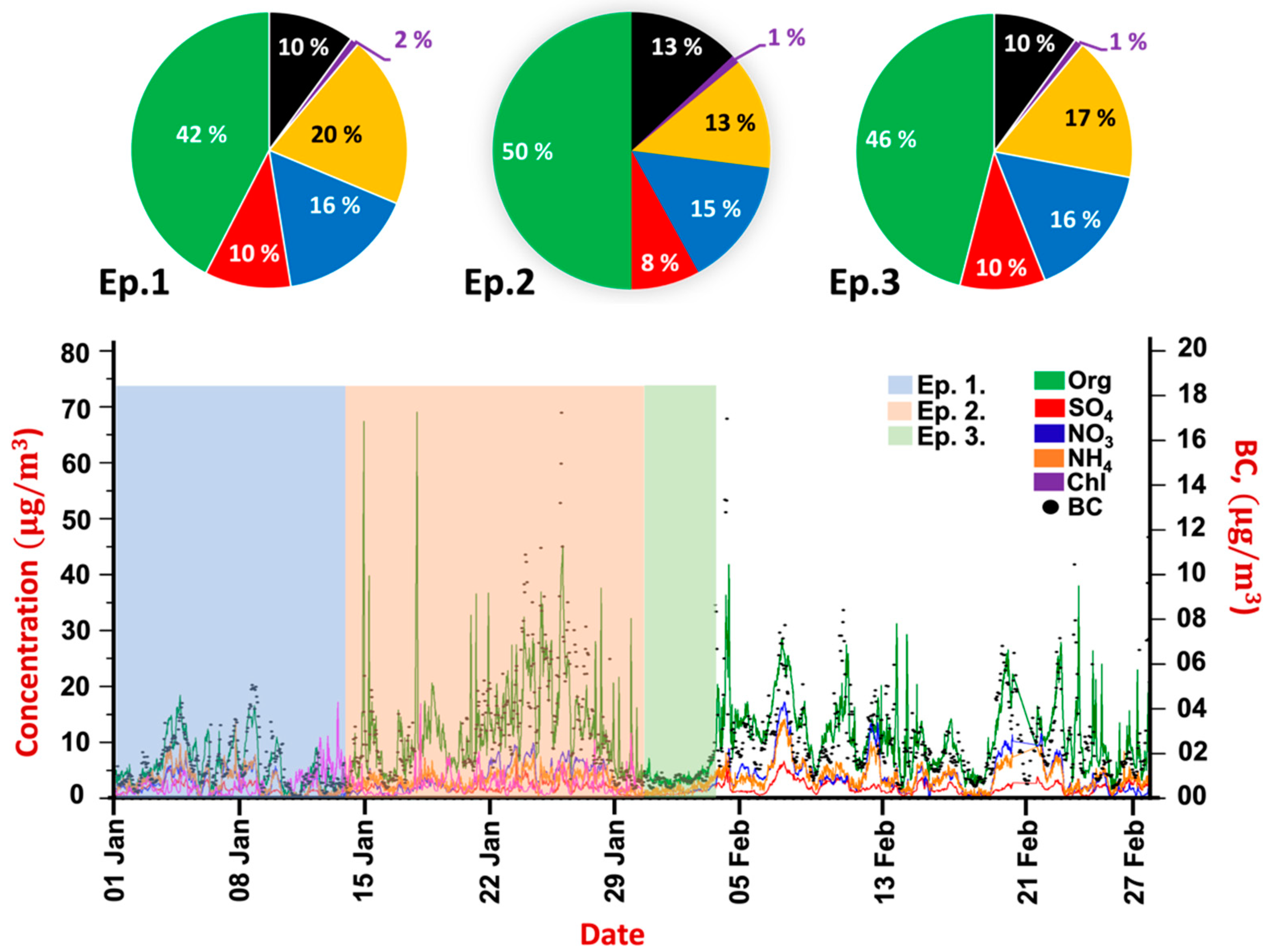
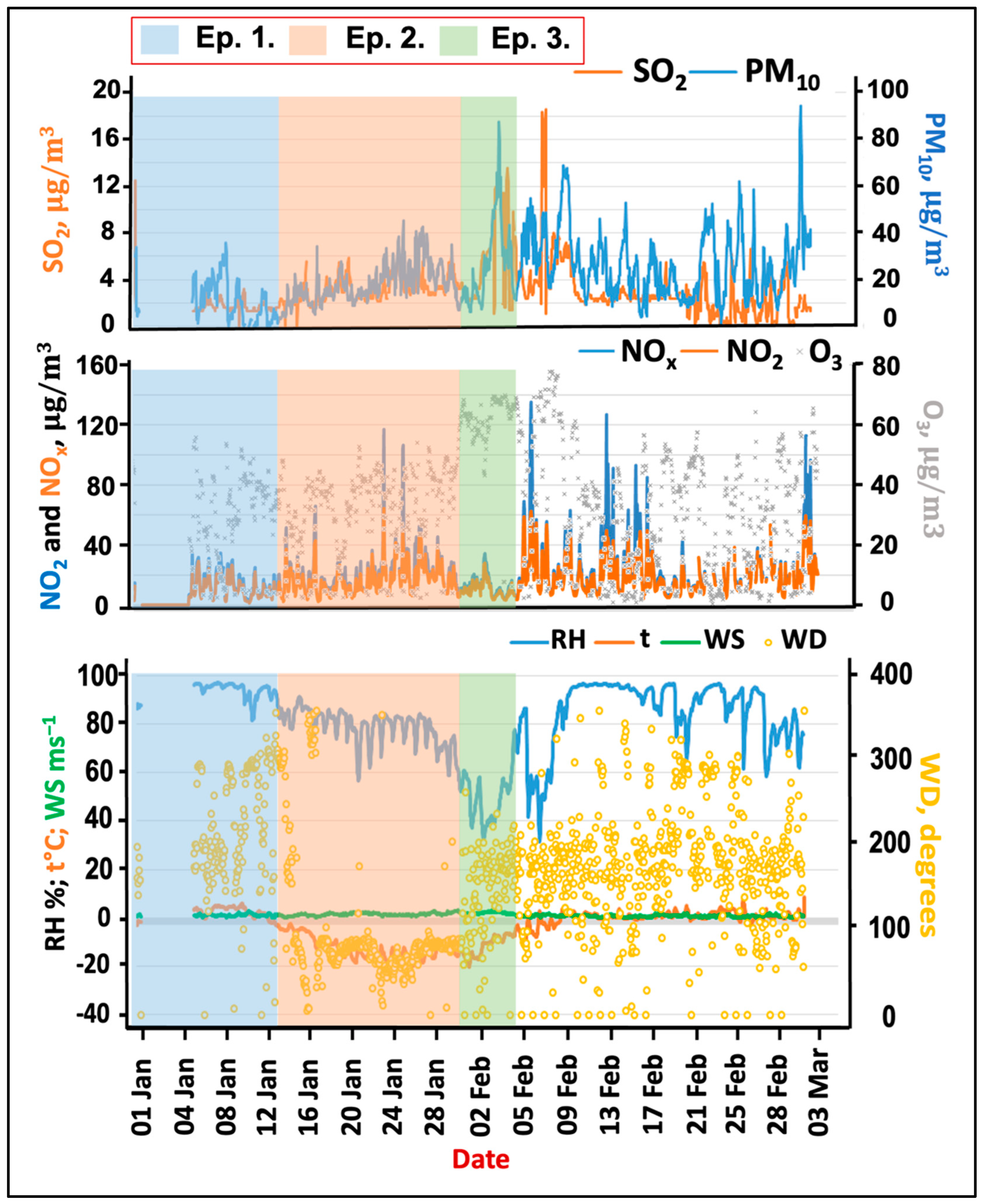
3.1. Overview
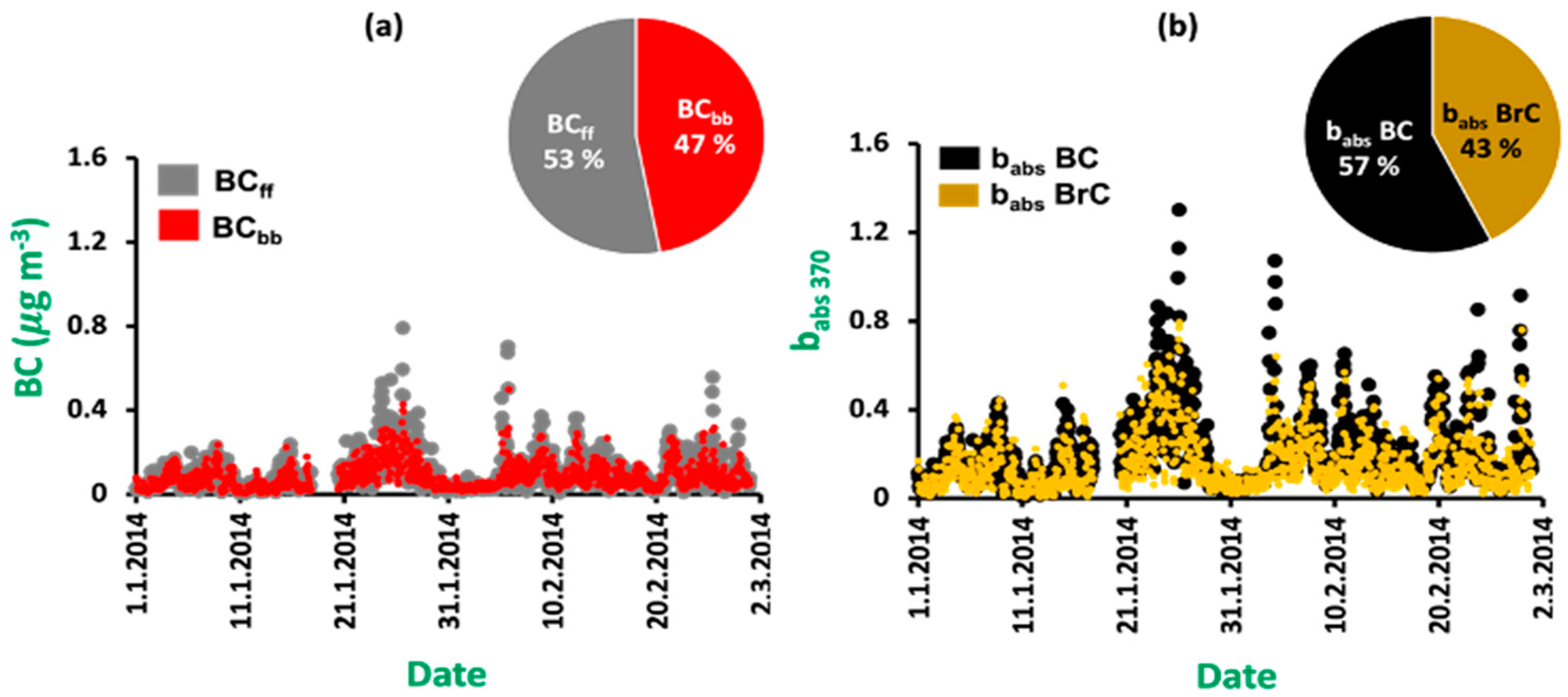
3.2. Source Apportionment of Ambient Black Carbon
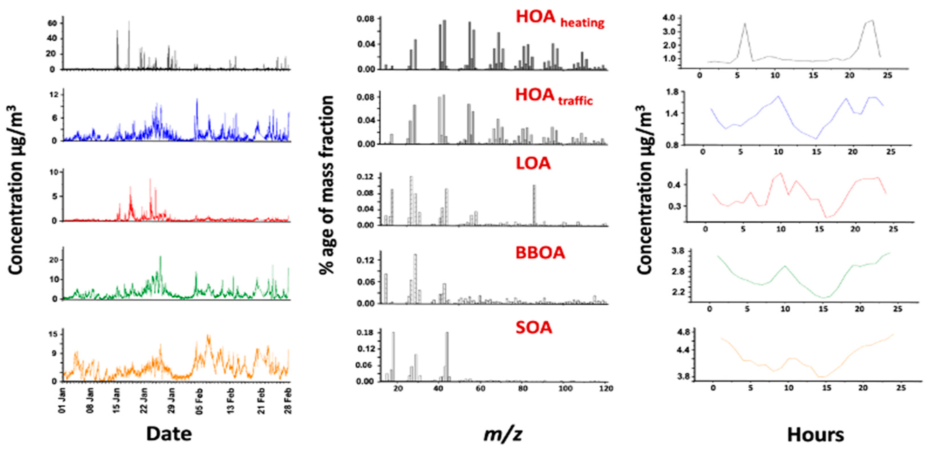
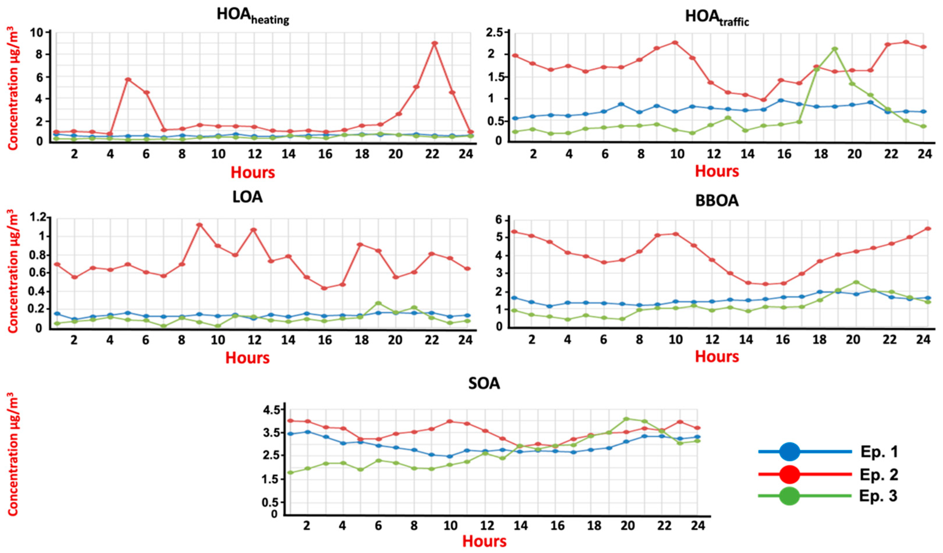
3.3. Source Apportionment of Ambient Organic Aerosol
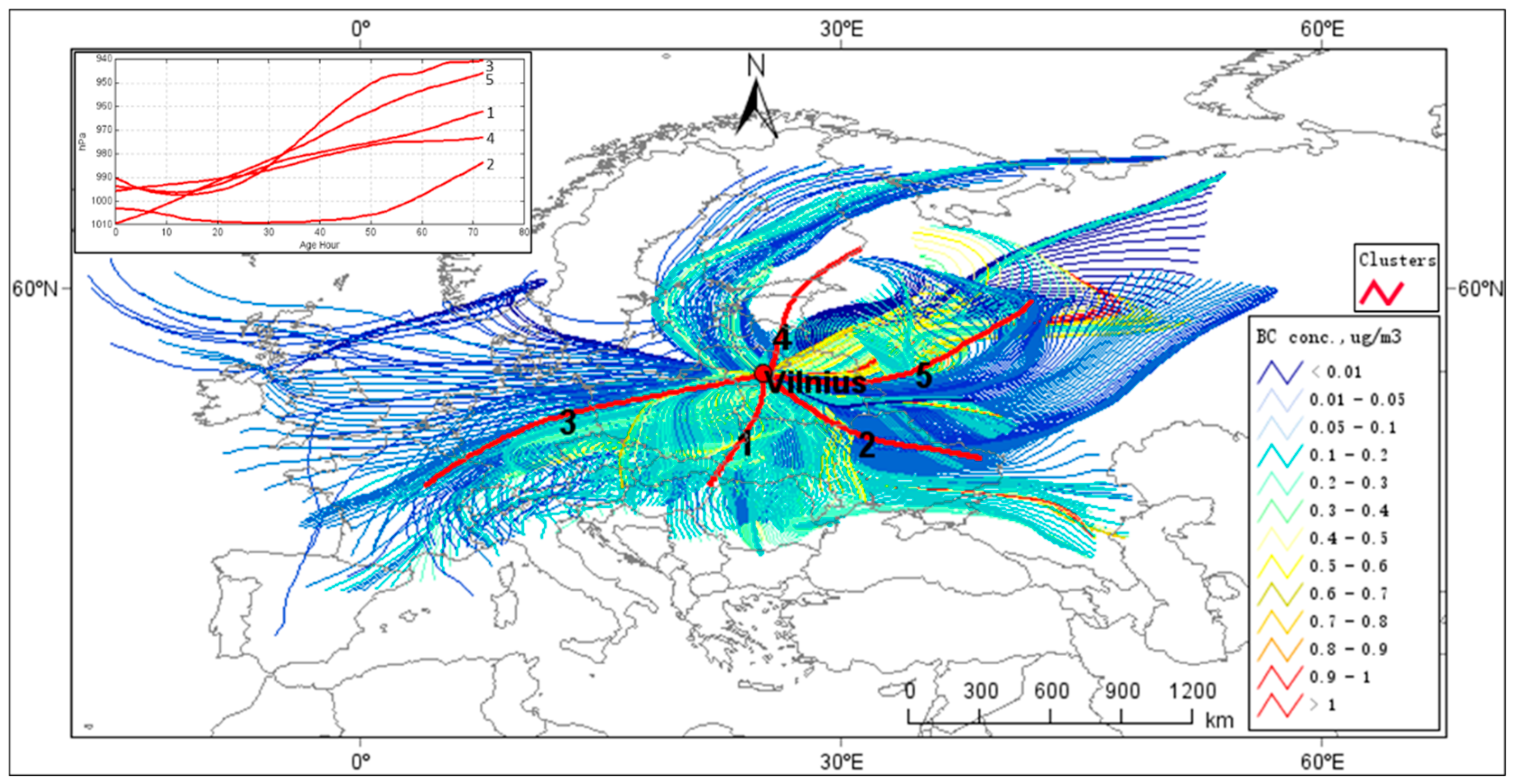
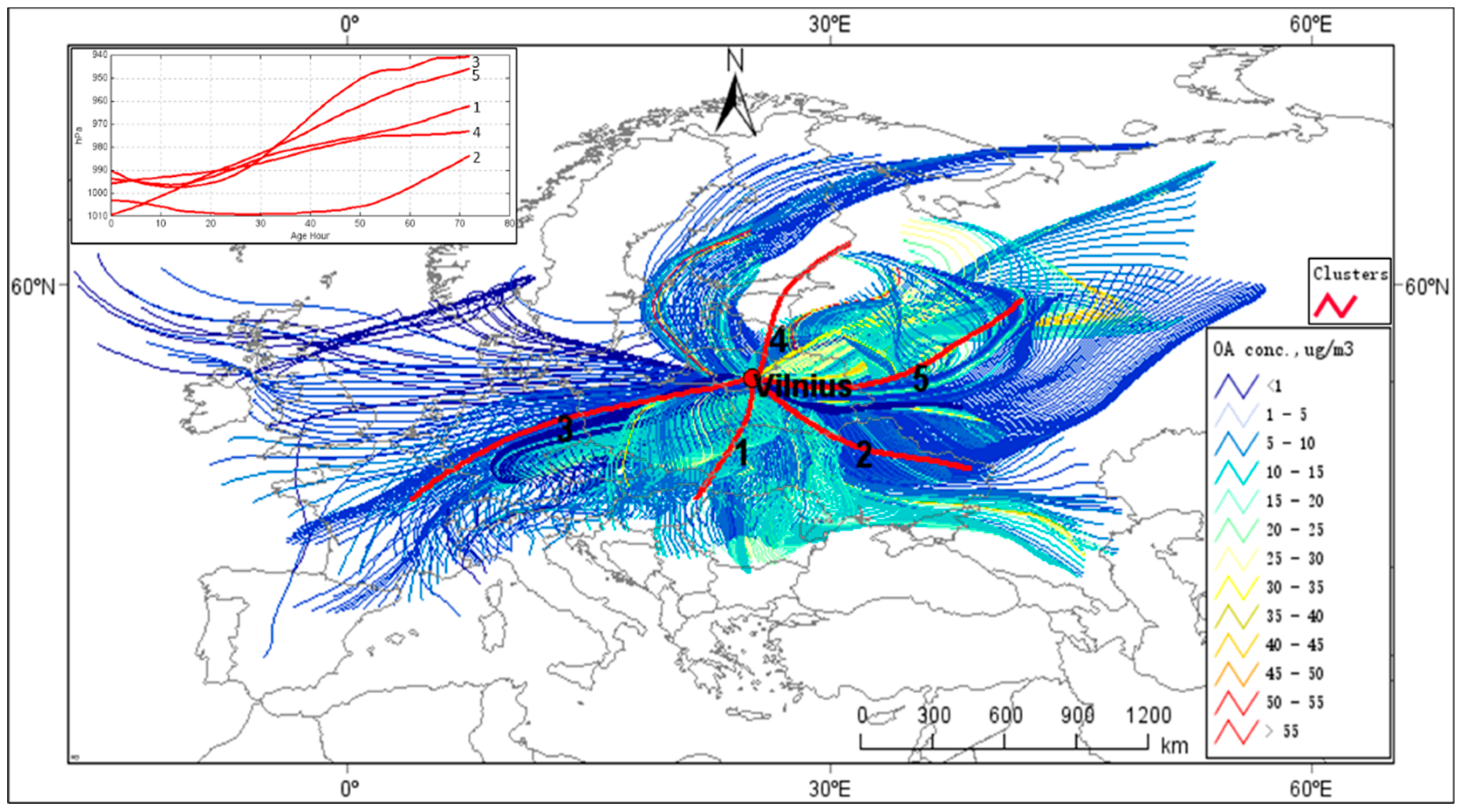
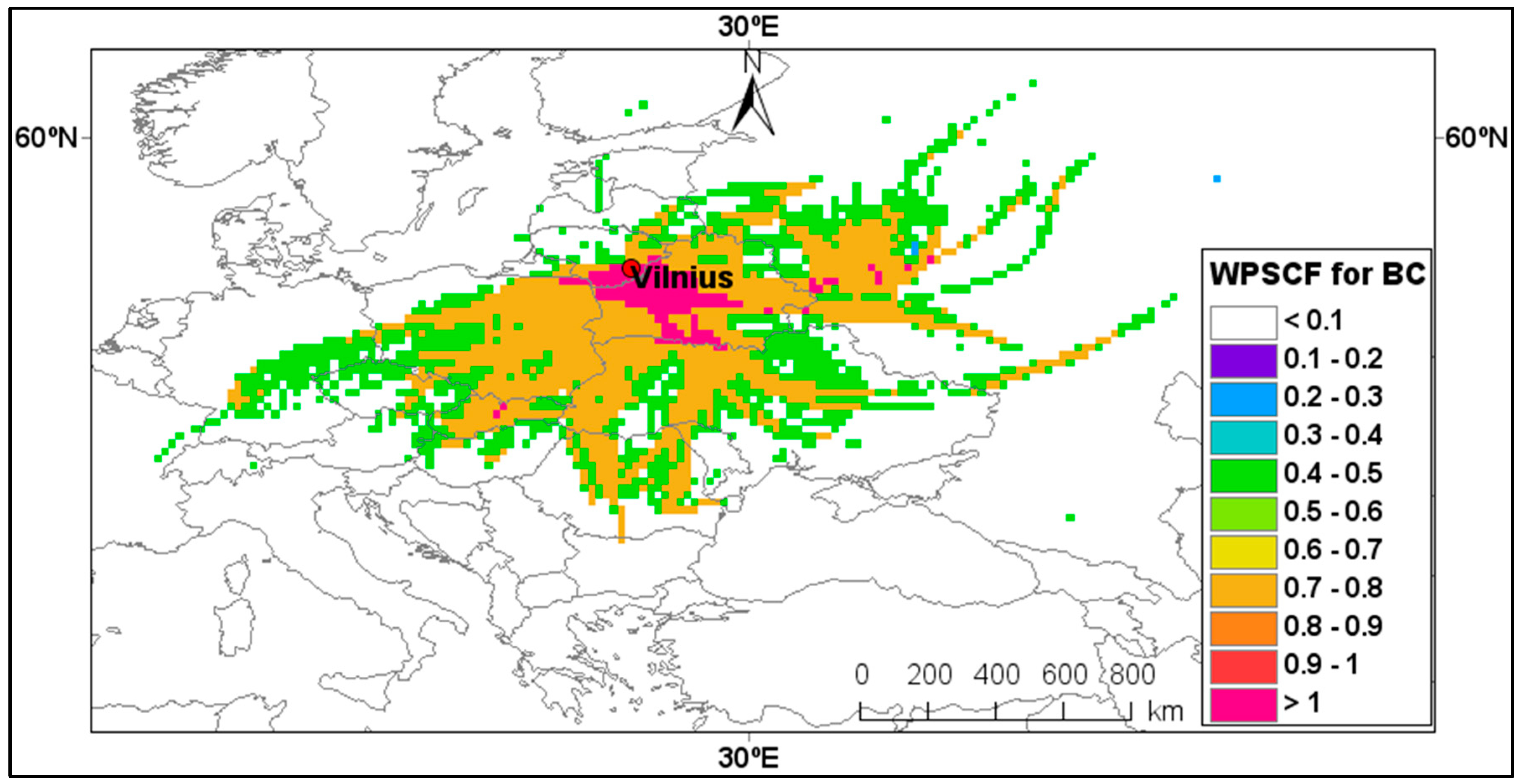
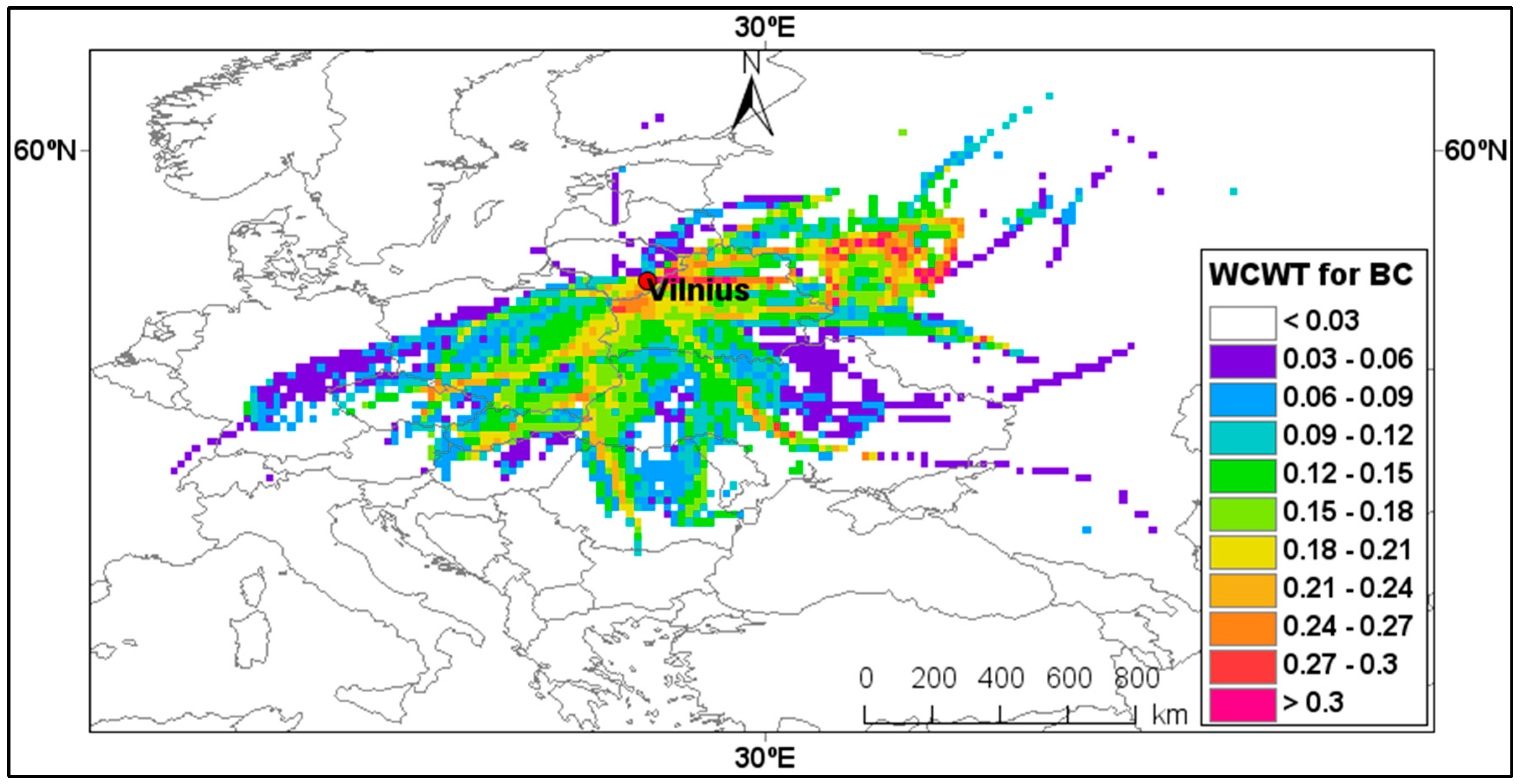
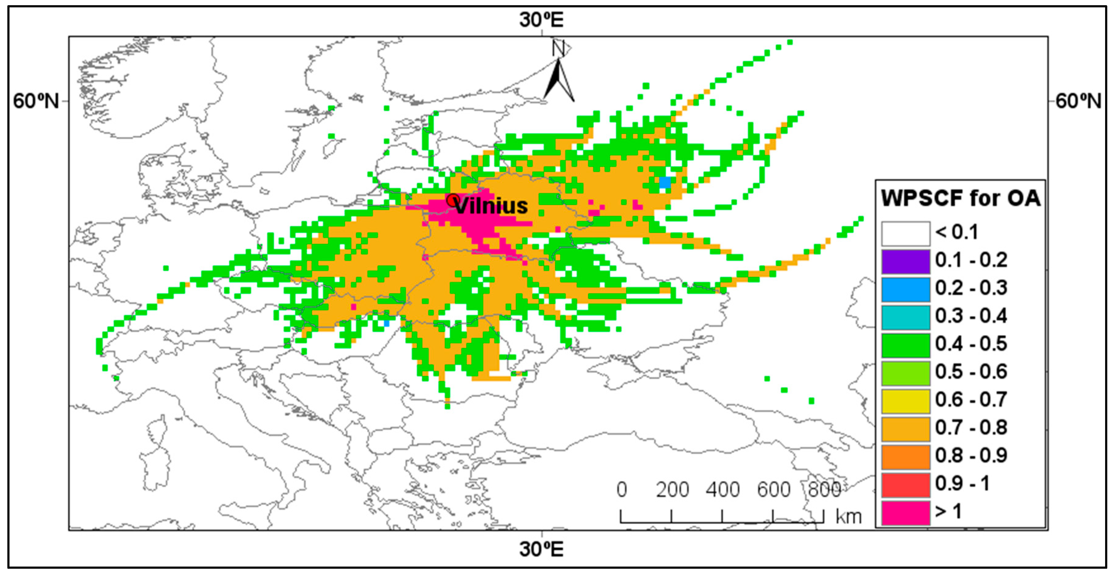
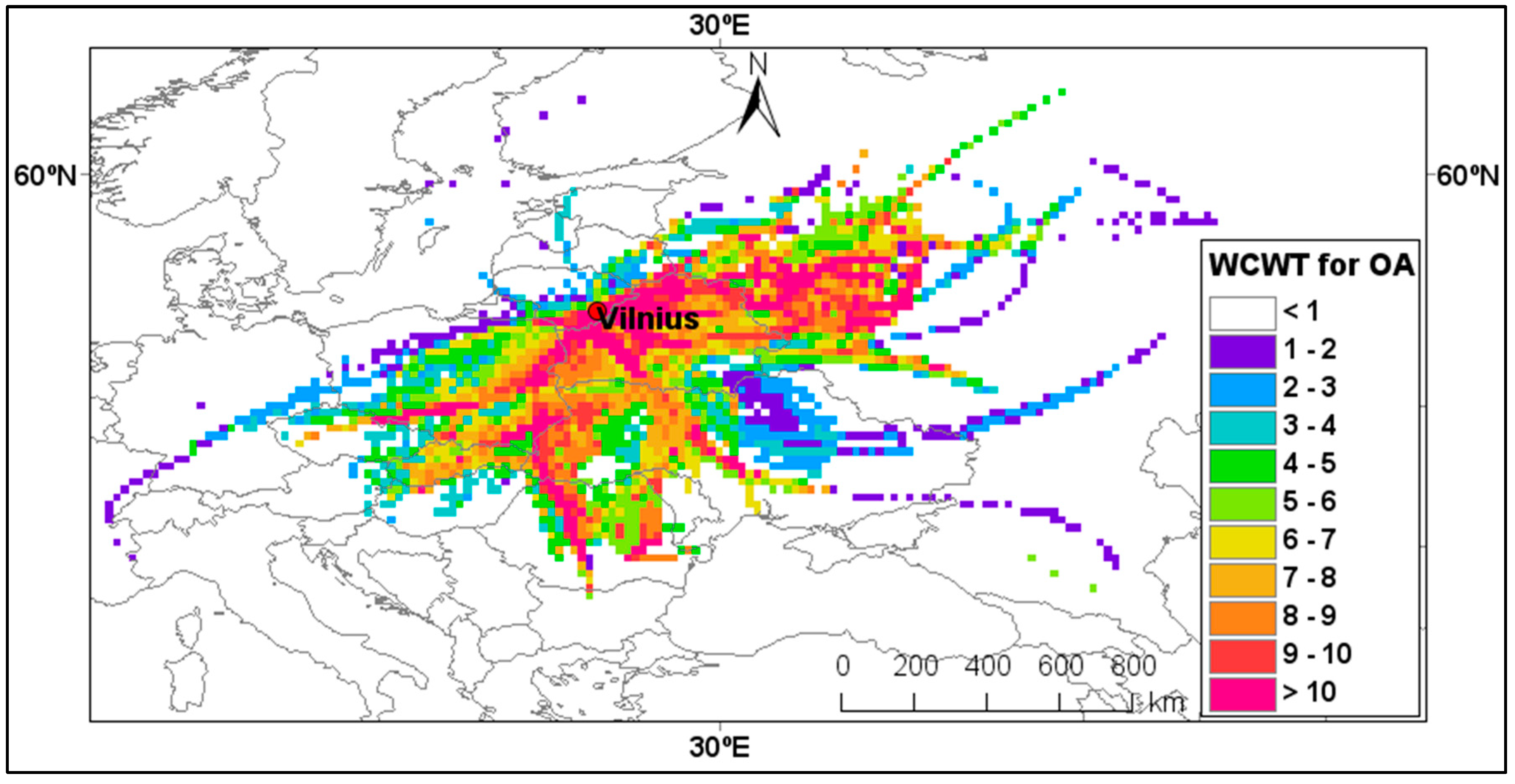
3.4. Impact of Air Masses on the Concentration Level of OA and BC
4. Conclusions
Author Contributions
Funding
Institutional Review Board Statement
Informed Consent Statement
Data Availability Statement
Acknowledgments
Conflicts of Interest
References
- Oh, H.J.; Ma, Y.; Kim, J. Human inhalation exposure to aerosol and health effect: Aerosol monitoring and modelling regional deposited doses. Int. J. Environ. Res. Public Health 2020, 17, 1923. [Google Scholar] [CrossRef] [PubMed]
- Ouidir, M.; Seyve, E.; Rivière, E.; Bernard, J.; Cheminat, M.; Cortinovis, J.; Ducroz, F.; Dugay, F.; Hulin, A.; Kloog, I.; et al. Maternal ambient exposure to atmospheric pollutants during pregnancy and offspring term birth weight in the nationwide elfe cohort. Int. J. Environ. Res. Public Health 2021, 18, 5806. [Google Scholar] [CrossRef] [PubMed]
- WHO. WHO global air quality guidelines. Coast. Estuar. Process. 2021, 1–360. [Google Scholar]
- Lelieveld, J.; Evans, J.S.; Fnais, M.; Giannadaki, D.; Pozzer, A. The contribution of outdoor air pollution sources to premature mortality on a global scale. Nature 2015, 525, 367–371. [Google Scholar] [CrossRef] [PubMed]
- Cao, J.J.; Lee, S.C.; Ho, K.F.; Zhang, X.Y.; Zou, S.C.; Fung, K.; Chow, J.C.; Watson, J.G. Characteristics of carbonaceous aerosol in Pearl River Delta Region, China during 2001 winter period. Atmos. Environ. 2003, 37, 1451–1460. [Google Scholar] [CrossRef]
- Zou, C.; Wang, J.; Hu, K.; Li, J.; Yu, C.; Zhu, F.; Huang, H. Distribution characteristics and source apportionment of winter carbonaceous aerosols in a rural area in Shandong, China. Atmosphere 2022, 13, 1858. [Google Scholar] [CrossRef]
- Chung, C.E.; Ramanathan, V.; Decremer, D. Observationally constrained estimates of carbonaceous aerosol radiative forcing. Proc. Natl. Acad. Sci. USA 2012, 109, 11624–11629. [Google Scholar] [CrossRef]
- Ancelet, T.; Davy, P.K.; Trompetter, W.J.; Markwitz, A.; Weatherburn, D.C. Carbonaceous aerosols in a wood burning community in rural New Zealand. Atmos. Pollut. Res. 2013, 4, 245–249. [Google Scholar] [CrossRef]
- Pachauri, T.; Singla, V.; Satsangi, A.; Lakhani, A.; Kumari, K.M. Characterization of carbonaceous aerosols with special reference to episodic events at Agra, India. Atmos. Res. 2013, 128, 98–110. [Google Scholar] [CrossRef]
- Safai, P.D.; Raju, M.P.; Rao, P.S.P.; Pandithurai, G. Characterization of carbonaceous aerosols over the urban tropical location and a new approach to evaluate their climatic importance. Atmos. Environ. 2014, 92, 493–500. [Google Scholar] [CrossRef]
- Bisht, D.S.; Dumka, U.C.; Kaskaoutis, D.G.; Pipal, A.S.; Srivastava, A.K.; Soni, V.K.; Attri, S.D.; Sateesh, M.; Tiwari, S. Carbonaceous aerosols and pollutants over delhi urban environment: Temporal evolution, source apportionment and radiative forcing. Sci. Total Environ. 2015, 521, 431–445. [Google Scholar] [CrossRef]
- Pani, S.K.; Wang, S.H.; Lin, N.H.; Chantara, S.; Lee, C.T.; Thepnuan, D. Black carbon over an urban atmosphere in Northern Peninsular Southeast Asia: Characteristics, source apportionment, and associated health risks. Environ. Pollut. 2020, 259, 113871. [Google Scholar] [CrossRef]
- Lin, W.; Dai, J.; Liu, R.; Zhai, Y.; Yue, D.; Hu, Q. Integrated assessment of health risk and climate effects of black carbon in the Pearl River Delta Region, China. Environ. Res. 2019, 176, 108522. [Google Scholar] [CrossRef] [PubMed]
- Mauderly, J.L.; Chow, J.C. Health effects of organic aerosols. Inhal. Toxicol. 2008, 20, 257–288. [Google Scholar] [CrossRef] [PubMed]
- Daniele, C.; Vechhi, R.; Viana, M. Carbonaceous aerosols in the atmosphere. Atmosphere 2018, 9, 181. [Google Scholar] [CrossRef]
- Diapouli, E.; Kalogridis, A.C.; Markantonaki, C.; Vratolis, S.; Fetfatzis, P.; Colombi, C.; Eleftheriadis, K. Annual variability of black carbon concentrations originating from biomass and fossil fuel combustion for the suburban aerosol in Athens, Greece. Atmosphere 2017, 8, 234. [Google Scholar] [CrossRef]
- Klejnowski, K.; Janoszka, K.; Czaplicka, M. Characterization and seasonal variations of organic and elemental carbon and levoglucosan in PM10 in Krynica Zdroj, Poland. Atmosphere 2017, 8, 190. [Google Scholar] [CrossRef]
- Minderytė, A.; Pauraite, J.; Dudoitis, V.; Plauškaitė, K.; Kilikevičius, A.; Matijošius, J.; Rimkus, A.; Kilikevičienė, K.; Vainorius, D.; Byčenkienė, S. Carbonaceous aerosol source apportionment and assessment of transport-related pollution. Atmos. Environ. 2022, 279, 119043. [Google Scholar] [CrossRef]
- Goss, M.; Swain, D.L.; Abatzoglou, J.T.; Sarhadi, A.; Kolden, C.A.; Williams, A.P.; Diffenbaugh, N.S. Climate change is increasing the likelihood of extreme autumn wildfire conditions across California. Environ. Res. Lett. 2020, 15, 094016. [Google Scholar] [CrossRef]
- Kirchmeier-Young, M.C.; Gillett, N.P.; Zwiers, F.W.; Cannon, A.J.; Anslow, F.S. Attribution of the influence of human-induced climate change on an extreme fire season. Earth’s Future 2019, 7, 2–10. [Google Scholar] [CrossRef] [PubMed]
- Hamilton, R.S.; Mansfield, T.A. Airborne particulate elemental carbon: Its sources, transport and contribution to dark smoke and soiling. Atmos. Environ. Part A Gen. Top. 1991, 25, 715–723. [Google Scholar] [CrossRef]
- Briggs, N.L.; Long, C.M. Critical review of black carbon and elemental carbon source apportionment in Europe and the United States. Atmos. Environ. 2016, 144, 409–427. [Google Scholar] [CrossRef]
- Popovicheva, O.; Ivanov, A.; Vojtisek, M. Functional factors of biomass burning contribution to spring aerosol composition in a Megacity: Combined ftir-pca analyses. Atmosphere 2020, 11, 319. [Google Scholar] [CrossRef]
- Chernyshev, V.V.; Zakharenko, A.M.; Ugay, S.M.; Hien, T.T.; Hai, L.H.; Kholodov, A.S.; Burykina, T.I.; Stratidakis, A.K.; Mezhuev, Y.O.; Tsatsakis, A.M.; et al. Morphologic and chemical composition of particulate matter in motorcycle engine exhaust. Toxicol. Rep. 2018, 5, 224–230. [Google Scholar] [CrossRef]
- Chernyshev, V.V.; Zakharenko, A.M.; Ugay, S.M.; Hien, T.T.; Hai, L.H.; Olesik, S.M.; Kholodov, A.S.; Zubko, E.; Kokkinakis, M.; Burykina, T.I.; et al. Morphological and chemical composition of particulate matter in buses exhaust. Toxicol. Rep. 2019, 6, 120–125. [Google Scholar] [CrossRef]
- Reddington, C.L.; McMeeking, G.; Mann, G.W.; Coe, H.; Frontoso, M.G.; Liu, D.; Flynn, M.; Spracklen, D.V.; Carslaw, K.S. The mass and number size distributions of black carbon aerosol over Europe. Atmos. Chem. Phys. 2013, 13, 4917–4939. [Google Scholar] [CrossRef]
- Ceolato, R.; Bedoya-Velásquez, A.E.; Fossard, F.; Mouysset, V.; Paulien, L.; Lefebvre, S.; Mazzoleni, C.; Sorensen, C.; Berg, M.J.; Yon, J. Black carbon aerosol Number and mass concentration measurements by picosecond short-range elastic backscatter lidar. Sci. Rep. 2022, 12, 8443. [Google Scholar] [CrossRef] [PubMed]
- Weagle, C.L.; Snider, G.; Li, C.; Van Donkelaar, A.; Philip, S.; Bissonnette, P.; Burke, J.; Jackson, J.; Latimer, R.; Stone, E.; et al. Global sources of fine particulate matter: Interpretation of PM2.5 chemical composition observed by SPARTAN using a global chemical transport model. Environ. Sci. Technol. 2018, 52, 11670–11681. [Google Scholar] [CrossRef] [PubMed]
- Kwon, H.S.; Ryu, M.H.; Carlsten, C. Ultrafine particles: Unique physicochemical properties relevant to health and disease. Exp. Mol. Med. 2020, 52, 318–328. [Google Scholar] [CrossRef]
- Wang, C.; Ye, Z.; Yu, Y.; Gong, W. Estimation of bus emission models for different fuel types of buses under real conditions. Sci. Total Environ. 2018, 640, 965–972. [Google Scholar] [CrossRef]
- Shan, X.; Chen, X.; Jia, W.; Ye, J. Evaluating urban bus emission characteristics based on localized MOVES using Sparse GPS data in Shanghai, China. Sustainability 2019, 11, 2936. [Google Scholar] [CrossRef] [Green Version]
- Byčenkienė, S.; Khan, A.; Bimbaitė, V. Impact of PM2.5 and PM10 emissions on changes of their concentration levels in Lithuania: A case study. Atmosphere 2022, 13, 1793. [Google Scholar] [CrossRef]
- Jonidi Jafari, A.; Charkhloo, E.; Pasalari, H. Urban Air Pollution Control Policies and Strategies: A Systematic Review; Springer International Publishing: Berlin/Heidelberg, Germany, 2021; Volume 19, ISBN 0123456789. [Google Scholar]
- Triantafyllopoulos, G.; Dimaratos, A.; Ntziachristos, L.; Bernard, Y.; Dornoff, J.; Samaras, Z. A Study on the CO2 and NOx emissions performance of Euro 6 diesel vehicles under various chassis dynamometer and on-road conditions including latest regulatory provisions. Sci. Total Environ. 2019, 666, 337–346. [Google Scholar] [CrossRef] [PubMed]
- Brewer, T.L. Black carbon emissions and regulatory policies in transportation. Energy Policy 2019, 129, 1047–1055. [Google Scholar] [CrossRef]
- Grigoratos, T.; Fontaras, G.; Giechaskiel, B.; Zacharof, N. Real world emissions performance of heavy-duty euro vi diesel vehicles. Atmos. Environ. 2019, 201, 348–359. [Google Scholar] [CrossRef]
- Lurkin, V.; Hambuckers, J.; van Woensel, T. Urban low emissions zones: A behavioral operations management perspective. Transp. Res. Part A Policy Pract. 2021, 144, 222–240. [Google Scholar] [CrossRef]
- Trojanowski, R.; Fthenakis, V. Nanoparticle emissions from residential wood combustion: A critical literature review, characterization, and recommendations. Renew. Sustain. Energy Rev. 2019, 103, 515–528. [Google Scholar] [CrossRef]
- Ng, N.L.; Herndon, S.C.; Trimborn, A.; Canagaratna, M.R.; Croteau, P.L.; Onasch, T.B.; Sueper, D.; Worsnop, D.R.; Zhang, Q.; Sun, Y.L.; et al. An aerosol chemical speciation monitor (ACSM) for routine monitoring of the composition and mass concentrations of ambient aerosol. Aerosol Sci. Technol. 2011, 45, 780–794. [Google Scholar] [CrossRef]
- Middlebrook, A.M.; Bahreini, R.; Jimenez, J.L.; Canagaratna, M.R. Evaluation of composition-dependent collection efficiencies for the aerodyne aerosol mass spectrometer using field data. Aerosol Sci. Technol. 2012, 46, 258–271. [Google Scholar] [CrossRef]
- Canonaco, F.; Crippa, M.; Slowik, J.G.; Baltensperger, U.; Prévôt, A.S.H. SoFi, an IGOR-based interface for the efficient use of the generalized multilinear engine (ME-2) for the source apportionment: ME-2 application to aerosol mass spectrometer data. Atmos. Meas. Tech. 2013, 6, 3649–3661. [Google Scholar] [CrossRef]
- Helin, A.; Niemi, J.V.; Virkkula, A.; Pirjola, L.; Teinilä, K.; Backman, J.; Aurela, M.; Saarikoski, S.; Rönkkö, T.; Asmi, E.; et al. Characteristics and source apportionment of black carbon in the Helsinki Metropolitan area, Finland. Atmos. Environ. 2018, 190, 87–98. [Google Scholar] [CrossRef]
- Liu, C.; Chung, C.E.; Yin, Y.; Schnaiter, M. The absorption Ångström exponent of black carbon: From numerical aspects. Atmos. Chem. Phys. 2018, 18, 6259–6273. [Google Scholar] [CrossRef]
- Weingartner, E.; Saathoff, H.; Schnaiter, M.; Streit, N.; Bitnar, B.; Baltensperger, U. Absorption of light by soot particles: Determination of the absorption coefficient by means of aethalometers. J. Aerosol Sci. 2003, 34, 1445–1463. [Google Scholar] [CrossRef]
- Zotter, P.; Herich, H.; Gysel, M.; El-Haddad, I.; Zhang, Y.; Mocnik, G.; Hüglin, C.; Baltensperger, U.; Szidat, S.; Prévôt, A.S.H. Evaluation of the absorption Ångström exponents for traffic and wood burning in the aethalometer-based source apportionment using radiocarbon measurements of ambient aerosol. Atmos. Chem. Phys. 2017, 17, 4229–4249. [Google Scholar] [CrossRef]
- Paatero, P. Least squares formulation of robust non-negative factor analysis. Chemom. Intell. Lab. Syst. 1997, 37, 23–35. [Google Scholar] [CrossRef]
- Crippa, M.; Canonaco, F.; Lanz, V.A.; Äijälä, M.; Allan, J.D.; Carbone, S.; Capes, G.; Ceburnis, D.; Dall’Osto, M.; Day, D.A.; et al. Organic aerosol components derived from 25 AMS data sets across Europe Using a consistent ME-2 based source apportionment approach. Atmos. Chem. Phys. 2014, 14, 6159–6176. [Google Scholar] [CrossRef]
- Sandradewi, J.; Prévôt, A.S.H.; Weingartner, E.; Schmidhauser, R.; Gysel, M.; Baltensperger, U. A study of wood burning and traffic aerosols in an Alpine valley using a multi-wavelength aethalometer. Atmos. Environ. 2008, 42, 101–112. [Google Scholar] [CrossRef]
- Qin, Y.M.; Bo Tan, H.; Li, Y.J.; Jie Li, Z.; Schurman, M.I.; Liu, L.; Wu, C.; Chan, C.K. chemical characteristics of brown carbon in atmospheric particles at a suburban site near Guangzhou, China. Atmos. Chem. Phys. 2018, 18, 16409–16418. [Google Scholar] [CrossRef]
- Pauraite, J.; Mainelis, G.; Kecorius, S.; Minderytė, A.; Dudoitis, V.; Garbarienė, I.; Plauškaitė, K.; Ovadnevaite, J.; Byčenkienė, S. Office indoor PM and BC level in Lithuania: The role of a long-range smoke transport Event. Atmosphere 2021, 12, 1047. [Google Scholar] [CrossRef]
- Sun, Y.L.; Zhang, Q.; Schwab, J.J.; Demerjian, K.L.; Chen, W.N.; Bae, M.S.; Hung, H.M.; Hogrefe, O.; Frank, B.; Rattigan, O.V.; et al. Characterization of the sources and processes of organic and inorganic aerosols in New York City with a high-resolution time-of-flight aerosol mass apectrometer. Atmos. Chem. Phys. 2011, 11, 1581–1602. [Google Scholar] [CrossRef]
- Saarikoski, S.; Niemi, J.V.; Aurela, M.; Pirjola, L.; Kousa, A.; Rönkkö, T.; Timonen, H. Sources of black carbon at residential and traffic environments obtained by two source apportionment methods. Atmos. Chem. Phys. 2021, 21, 14851–14869. [Google Scholar] [CrossRef]
- Paatero, P.; Tapper, U. Positive matrix factorization: A non-negative factor model with optimal utilization of error estimates of data values. Environmetrics 1994, 5, 111–126. [Google Scholar] [CrossRef]
- Paglione, M.; Gilardoni, S.; Rinaldi, M.; Decesari, S.; Zanca, N.; Sandrini, S.; Giulianelli, L.; Bacco, D.; Ferrari, S.; Poluzzi, V.; et al. The impact of biomass burning and aqueous-phase processing on air quality: A multi-year source apportionment study in the Po Valley, Italy. Atmos. Chem. Phys. 2020, 20, 1233–1254. [Google Scholar] [CrossRef]
- Wang, Y.Q.; Zhang, X.Y.; Draxler, R.R. TrajStat: GIS-Based software that uses various trajectory statistical analysis methods to identify potential sources from long-term air pollution measurement data. Environ. Model. Softw. 2009, 24, 938–939. [Google Scholar] [CrossRef]
- Guo, Y.; Lin, C.; Li, J.; Wei, L.; Ma, Y.; Yang, Q.; Li, D.; Wang, H.; Shen, J. Persistent pollution episodes, transport pathways, and potential sources of air pollution during the heating season of 2016–2017 in Lanzhou, China. Environ. Monit. Assess. 2021, 193, 852. [Google Scholar] [CrossRef]
- Hsu, Y.K.; Holsen, T.M.; Hopke, P.K. Comparison of hybrid receptor models to locate pcb sources in Chicago. Atmos. Environ. 2003, 37, 545–562. [Google Scholar] [CrossRef]
- Draxler, R.R.; Hess, G.D. An overview of the hysplit_4 modelling system for trajectories, dispersion and deposition. Aust. Meteorol. Mag. 1998, 47, 295–308. [Google Scholar]
- Teinilä, K.; Aurela, M.; Niemi, J.V.; Kousa, A.; Petäjä, T.; Järvi, L.; Hillamo, R.; Kangas, L.; Saarikoski, S.; Timonen, H. Concentration variation of gaseous and particulate pollutants in the helsinki city centre—Observations from a two-year campaign from 2013–2015. Boreal Environ. Res. 2019, 24, 115–136. [Google Scholar]
- Calvo, A.I.; Alves, C.; Castro, A.; Pont, V.; Vicente, A.M.; Fraile, R. Research on aerosol sources and chemical composition: Past, current and emerging issues. Atmos. Res. 2013, 121, 1–28. [Google Scholar] [CrossRef]
- Li, X.; Zhao, Q.; Yang, Y.; Zhao, Z.; Liu, Z.; Wen, T.; Hu, B.; Wang, Y.; Wang, L.; Wang, G. Composition and sources of brown carbon aerosols in Megacity Beijing during the winter of 2016. Atmos. Res. 2021, 262, 105773. [Google Scholar] [CrossRef]
- Weitzel, K.; Chemie, F.; Rev, M.S.; Introduction, I.; Reference, C. Bond-dissociation energies of cations—Pushing the limits to quantum state resolution. WHO Libr. Cat. Data 2011, 221–235. [Google Scholar] [CrossRef] [PubMed]
- Thepnuan, D.; Chantara, S.; Lee, C.T.; Lin, N.H.; Tsai, Y.I. Molecular markers for biomass burning associated with the characterization of PM2.5 and component sources during dry season haze episodes in upper South East Asia. Sci. Total Environ. 2019, 658, 708–722. [Google Scholar] [CrossRef] [PubMed]
- Weimer, S.; Alfarra, M.R.; Schreiber, D.; Mohr, M.; Prévôt, A.S.H.; Baltensperger, U. Organic aerosol mass spectral signatures from wood-burning emissions: Influence of burning conditions and type. J. Geophys. Res. Atmos. 2008, 113, D10304. [Google Scholar] [CrossRef] [Green Version]
- May, N.; Kuo, L.; Caby, E.A. Bootstrap Methods and Their Application. ASQ 2014, 42, 216–217. [Google Scholar] [CrossRef]
- Berriban, I.; Azahra, M.; Chham, E.; Ferro-García, M.A.; Milena-Pérez, A.; Nouayti, A.; Orza, J.A.G.; Brattich, E.; Tositti, L.; Piñero-García, F.; et al. PSCF and CWT Methods as a Tool to Identify Potential sources of 7Be and 210Pb aerosols in Granada, Spain. J. Environ. Radioact. 2022, 251, 106977. [Google Scholar] [CrossRef] [PubMed]


| HOAheating | HOAtraffic | LOA | BBOA | SOA | |||||||||||
|---|---|---|---|---|---|---|---|---|---|---|---|---|---|---|---|
| Day | Night | Diff | Day | Night | Diff | Day | Night | Diff | Day | Night | Diff | Day | Night | Diff | |
| Ep. 1. | 0.55 | 0.57 | 3% | 0.79 | 0.69 | −15% | 0.13 | 0.14 | 6% | 1.50 | 1.56 | 3% | 2.73 | 3.28 | 17% |
| Ep. 2. | 1.46 | 3.11 | 53% | 1.60 | 1.88 | 15% | 0.75 | 0.66 | −13% | 3.66 | 4.72 | 22% | 3.40 | 3.71 | 9% |
| Ep. 3. | 0.41 | 0.38 | −9% | 0.59 | 0.53 | −12% | 0.10 | 0.10 | 7% | 1.06 | 1.27 | 16% | 2.60 | 2.79 | 7% |
| Whole period | 1.12 | 1.54 | 28% | 1.33 | 1.39 | 5% | 0.35 | 0.37 | 6% | 2.58 | 3.25 | 21% | 4.06 | 4.50 | 10% |
| General Statistics of Clusters | Trajectories of BC | Trajectories of OA | ||||||
|---|---|---|---|---|---|---|---|---|
| Cluster no. | No. of trajectories | Ratio to all trajectories | No. of trajectories | Mean conc., µg/m3 | Standard deviation | No. of trajectories | Mean conc., µg/m3 | Standard deviation |
| 1 | 479 | 33.83% | 479 | 0.21 | 0.12 | 473 | 11.15 | 5.85 |
| 2 | 266 | 18.79% | 264 | 0.19 | 0.19 | 254 | 9.60 | 6.26 |
| 3 | 192 | 13.56% | 192 | 0.11 | 0.09 | 164 | 4.90 | 3.59 |
| 4 | 132 | 9.32% | 120 | 0.12 | 0.09 | 132 | 8.04 | 8.49 |
| 5 | 347 | 24.51% | 297 | 0.25 | 0.21 | 346 | 12.27 | 8.03 |
| Total | 1416 | 100.01% | 1352 | 0.19 | 0.16 | 1369 | 10.10 | 7.00 |
Disclaimer/Publisher’s Note: The statements, opinions and data contained in all publications are solely those of the individual author(s) and contributor(s) and not of MDPI and/or the editor(s). MDPI and/or the editor(s) disclaim responsibility for any injury to people or property resulting from any ideas, methods, instructions or products referred to in the content. |
© 2023 by the authors. Licensee MDPI, Basel, Switzerland. This article is an open access article distributed under the terms and conditions of the Creative Commons Attribution (CC BY) license (https://creativecommons.org/licenses/by/4.0/).
Share and Cite
Byčenkienė, S.; Gill, T.; Khan, A.; Kalinauskaitė, A.; Ulevicius, V.; Plauškaitė, K. Estimation of Carbonaceous Aerosol Sources under Extremely Cold Weather Conditions in an Urban Environment. Atmosphere 2023, 14, 310. https://doi.org/10.3390/atmos14020310
Byčenkienė S, Gill T, Khan A, Kalinauskaitė A, Ulevicius V, Plauškaitė K. Estimation of Carbonaceous Aerosol Sources under Extremely Cold Weather Conditions in an Urban Environment. Atmosphere. 2023; 14(2):310. https://doi.org/10.3390/atmos14020310
Chicago/Turabian StyleByčenkienė, Steigvilė, Touqeer Gill, Abdullah Khan, Audrė Kalinauskaitė, Vidmantas Ulevicius, and Kristina Plauškaitė. 2023. "Estimation of Carbonaceous Aerosol Sources under Extremely Cold Weather Conditions in an Urban Environment" Atmosphere 14, no. 2: 310. https://doi.org/10.3390/atmos14020310