Article

Scale-Dependent Verification of the OU MAP Convection Allowing Ensemble Initialized with Multi-Scale and Large-Scale Perturbations during the 2019 NOAA Hazardous Weather Testbed Spring Forecasting Experiment

School of Meteorology, University of Oklahoma, Norman, OK 73072, USA
*
Author to whom correspondence should be addressed.
Atmosphere 2023, 14(2), 255; https://doi.org/10.3390/atmos14020255
Submission received: 8 December 2022 / Revised: 17 January 2023 / Accepted: 24 January 2023 / Published: 28 January 2023
(This article belongs to the Special Issue Numerical Weather Prediction Models and Ensemble Prediction Systems)

Abstract

:
Given the large range of resolvable space and time scales in large-domain convection-allowing for ensemble forecasts, there is a need to better understand optimal initial-condition perturbation strategies to sample the forecast uncertainty across these space and time scales. This study investigates two initial-condition perturbation strategies for CONUS-domain ensemble forecasts that extend into the two-day forecast lead time using traditional and object-based verification methods. Initial conditions are perturbed either by downscaling perturbations from a coarser resolution ensemble (i.e., LARGE) or by adopting the analysis perturbations from a convective-scale, EnKF system (i.e., MULTI). It was found that MULTI had more ensemble spread than LARGE across all scales initially, while LARGE’s perturbation energy surpassed that of MULTI after 3 h and continued to maintain a surplus over MULTI for the rest of the 36h forecast period. Impacts on forecast bias were mixed, depending on the forecast lead time and forecast threshold. However, MULTI was found to be significantly more skillful than LARGE at early forecast hours for the meso-gamma and meso-beta scales (1–9h), which is a result of a larger and better-sampled ensemble spread at these scales. Despite having a smaller ensemble spread, MULTI was also significantly more skillful than LARGE on the meso-alpha scale during the 20–24h period due to a better spread-skill relation. MULTI’s performance on the meso-alpha scale was slightly worse than LARGE’s performance during the 6–12h period, as LARGE’s ensemble spread surpassed that of MULTI. The advantages of each method for different forecast aspects suggest that the optimal perturbation strategy may require a combination of both the MULTI and LARGE techniques for perturbing initial conditions in a large-domain, convection-allowing ensemble.

1. Introduction

Convection-allowing ensemble (CAE) prediction systems have been developed, operated, and evaluated in both experimental and operational settings [1,2,3,4,5,6,7,8,9,10]. A challenging aspect of CAEs is generating initial condition (IC) perturbations (ICPs) that properly sample IC errors to account for uncertainties in a wide range of spatial scales. The most common technique for generating ICPs in a CAE is to downscale coarse-resolution analyses or short-term forecasts directly onto the CAE grid [4,11,12,13,14]. This approach allows the large-scale component of the flow to be perturbed while keeping the small scales essentially unperturbed at the initial time. Consequently, realistic, small-scale perturbations are obtained only after a few hours of forecast model integration. Ensemble-based data assimilation (EDA) provides another way to generate CAE ICPs (e.g., [14,15]). Unlike the downscaling method, ICPs generated by EDA tend to sample the uncertainty at all scales resolved by the Numerical Weather Prediction (NWP) model. For example, the ensemble Kalman filter (EnKF) has been used directly on the convection-allowing grid with hourly [15] or 20-min [14] data assimilation (DA) cycling. EnKF has also been used together with the ensemble–variational (EnVAR) DA on the convection-allowing grid by recentering the EnKF perturbations around the EnVAR control analysis [9]. While EDA on the convection-allowing grid is generally believed to improve the sampling of convective-scale IC uncertainty, a direct comparison of the ensemble performance the to simple downscaling of coarser-resolution ICPs has been limited to the Observation System Simulation Experiment framework [16] or to relatively small domains and short forecast lead times [14].
Ref. [14], or JW20, produced a multi-scale ICP with an EDA of the same horizontal resolution (3 km) as the subsequent NWP forecasts. Their evaluations of 18h forecasts of ten selected cases in small-domain (1200 km × 1200 km) experiments concluded that multi-scale ICPs were superior to large-scale ICPs during early forecast hours, with a generally decreased advantage as the forecast hours increased. Due to the limited number of cases and the forecast duration and domain, it was unclear whether the decreased advantage of the multi-scale ICP over time was a result of convection dissipation or storms moving out of the domain and if/when it would regain advantage for newly initiated storms beyond day one.
The present study further investigates the multi-scale and large-scale ICPs for the CAE prediction. In our experimental design, forecast skill differences are attributed to differences in ICPs only. The forecast domain is sufficiently large to sample multi-scale spatial uncertainties from several kilometers to thousands of kilometers. Additionally, forecast cases contain many large-scale forcing scenarios and mesoscale environments. Specifically, this study examined twenty-five 36h forecasts from two ten-member ensembles over the CONUS domain produced by the Multiscale data Assimilation and Predictability (MAP) lab at the University of Oklahoma (OU) during the NOAA Hazardous Weather Testbed 2019 Spring Forecasting Experiment (SFE 2019, hwt.nssl.noaa.gov/sfe/2019/docs/HWT_SFE2019_operations_plan.pdf, accessed on 8 December 2022). The two ensembles were designed similarly to the ones in JW20, with one initialized by multi-scale ICPs derived from an EDA and the other initialized by large-scale ICPs downscaled from the Global Ensemble Forecast System (GEFS). The EDA of the OU MAP ensemble adopts the hybrid EnVar and EnKF DA systems [17]. The EnVar generates a deterministic control analysis. The recentered EnKF perturbations produce the sampling of IC errors. The system assimilates both the synoptic and meso-scale observations as well as the convective scale radar-reflectivity observations, following [18]. When compared to JW20, the increased number of cases and the larger CONUS domain allows for the thorough investigation of the differences of multi-scale and downscaled large-scale ICPs. In addition, the extended forecast period, from 18h to 36h, enables the exploration of the benefits of either large-scale or multi-scale ICPs for second-day forecasts.
To evaluate the impact of multi-scale and large-scale ICPs on storms of different spatial scales, the present study also introduces a new, scale-dependent verification framework. Specifically, the object-based storm tracking technique of [19] is applied to the observed reflectivity from the Multi-Radar Multi-Sensor (MRMS, [20]) and the simulated reflectivity from the two ensembles. The MRMS system combines radar-reflectivity from all NEXRAD radars to produce a gridded mosaic of composite reflectivity suitable for forecast verification [20]. The object-based storm time series are further classified into three different scales for verification. The structure of this paper is as follows: Section 2 describes the EDA system, the design of two CAEs and the new, scale-dependent verification framework. The verification results are presented in Section 3, and a summary is contained in Section 4.

2. Data and Methodology

2.1. OU MAP Ensembles during SFE 2019

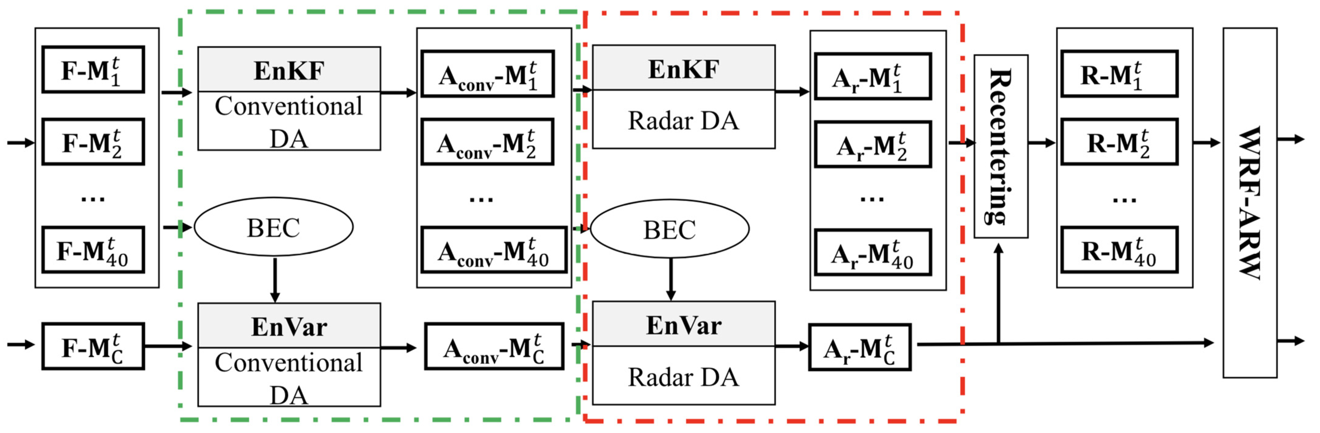
2.1.1. Ensemble Data Assimilation System

The EDA system used to initialize the OU MAP ensembles during the SFE 2019 was the GSI-based, ensemble-variational (EnVar) hybrid system based on the Advanced Research version of the Weather Research and Forecasting (WRF) Model (ARW; version 3.9; [21]), which directly assimilates both conventional (i.e., temperature, moisture, wind, and surface pressure from surface station, radiosonde, and aircraft observations) and radar-reflectivity observations (e.g., [18,22]). Conventional data were assimilated hourly during 1800-0000 UTC, and radar-reflectivity data were assimilated every 20 min from 2300 UTC to 0000 UTC. The density of conventional and radar observations is similar to that of Johnson et al. 2015 (their Figure 2). The conventional and radar DAs were separated into two steps to facilitate the differences in cycling intervals and localization length scales appropriate to the different observations and the corresponding scales of motion that they are capable of observing.
The EDA system contained forty members, including forty ensemble members updated by the GSI-based EnKF [23] and one control member updated by the GSI-based EnVar [18,24,25]. The Global Forecast System (GFS) control analysis and subsequent forecast provided the initial conditions (ICs) and lateral boundary conditions (LBCs) for EnVar control. The forty-member ensemble ICs and LBCs were constructed by adding the forty-member ensemble perturbations to the GFS control analysis and forecast. The forty-member ensemble perturbations were extracted from the GEFS and the Short-Range Ensemble Forecast (SREF) at the National Centers for Environmental Prediction (NCEP), as was similarly done in JW20.
Figure 1 presents the design of the EDA system for each DA cycle when both the conventional and radar-reflectivity observations were assimilated. The flow chart was expanded from [25,26]. The detailed procedure is introduced as follows:
(1) At the analysis time t, the EnKF and EnVar were first conducted to assimilate conventional observations. The ensemble first-guesses F- M k t , k = 1, 2, …, 40, and the control first-guesses F- M C t were updated using EnKF and EnVar to generate the ensemble analyses Aconv- M k t , k = 1, 2, …, 40, and the control analysis Aconv- M C t , respectively, in which subscript c indicates the conventional observations assimilation step. The ensemble firstguesses were used to estimate the background error covariances (BECs) for the EnVar update;
(2) Radar-reflectivity observations were then assimilated following a similar procedure in step (1). The analyses Aconv- M k t , k = 1, 2, …, 40, and Aconv- M C t served as the first guesses, and Aconv- M k t , k = 1, 2, …, 40, was used to estimate the BEC for the EnVar update. The EnVar direct radar reflectivity assimilation approach of Wang and Wang 2017 was adopted. The updated ensemble analyses through EnKF and the control analysis through EnVar were Ar- M k t , k = 1, 2, …, 40, and Ar- M C t , respectively, where subscript r indicates the radar observations assimilation step;
(3) The 40 EnKF members Ar- M k t , k = 1, 2, …, 40, were re-centered around the EnVar control to obtain the final ensemble analyses R- M k t , k = 1, 2, …, 40, for preventing divergence of the ensemble from the control;
(4) The short-term forecasts were performed to advance R- M k t , k = 1, 2, …, 40, and Ar- M C t to the next DA cycle, t + 1, through WRF-ARW.
If only conventional observations were available at cycle t, the procedure in the red box (Figure 1) was skipped. The same was true for the green box when only the radar observations were assimilated.
This system applied equivalent horizontal and vertical localization scales to the EnVar and EnKF. The assimilation of conventional observations used a horizontal cutoff distance of 300 km and a vertical distance of 0.55 scale height. The assimilation of radar observations used a horizontal cutoff distance of 15 km and a vertical distance of 1.1 scale height. The 15 km scale of horizontal localization for the radar observations was guided by the spacing of radar observations (~2 km) and was consistent with past studies assimilating radar reflectivity in the EnKF (e.g., JW20 and [9]). The relaxation to prior spread (RTPS; [27]) inflation method was used to retain 95% of the background ensemble spread in the ensemble analyses. Similar localization scales and RTPS coefficients were applied in JW20 and [9].
This system employed a CONUS-covering domain centered at 38.5 °N, 97.5 °W with a size of 1620 × 1120 × 50 grid points (Figure 2). The horizontal grid spacing was 3 km and the model top was 50 hPa. A fixed physics suite was used during DA and ensemble forecasts, including the Mellor–Yamada–Nakanishi–Niino [28] boundary layer parameterization, Thompson [29] microphysics parameterization, Rapid Update Cycle [30] land surface model, and Rapid Radiative Transfer Model [31] radiation parameterization.

2.1.2. IC Perturbation Methods

At 00z each day during SFE 2019, two 36-h, ten-member ensembles of 3 km resolution from the OU MAP lab were launched. The first ensemble was initialized from the EnKF analysis ensembles that were recentered on the EnVar control analysis. The second ensemble was initialized by adding the GEFS perturbations (i.e., each GEFS member minus the GEFS ensemble mean) to the same EnVar control analysis of the first ensemble. The GEFS perturbations were obtained from short-term (0–6h) forecasts from the operational global ensemble at the NCEP. By construction, the two ensembles only differed by their ICPs. The ensemble that directly uses the analysis perturbations from the EDA system is referred to as “MULTI”. As described in Section 2.1.1, the EDA performed data assimilation for multiple scales. The control EnVar analysis and recentered EnKF perturbations therefore intend to provide an estimate of the state and the uncertainty of such a state estimate for multiple resolved scales. The ensemble that downscales GEFS perturbations as ICPs is referred to as “LARGE”. Because the GEFS forecast grid spacing was 50 km, we would not expect the downscaled ICPs from GEFS to accurately resolve the analysis uncertainty on meso-beta (20~200 km) and meso-gamma (2~20 km) scales.
It is emphasized that both LARGE and MULTI share the same ensemble mean initial condition, and only differ in the ICPs from the mean that are added to each member. The ICPs for MULTI not only have a higher resolution than those for LARGE, but also have convective-scale, flow-dependent covariances resulting from the assimilation of radar-reflectivity observations. The goal of these experiments is to evaluate the impact of the convective-scale perturbation structure resulting from the EDA with radar observations, compared to ensemble forecasts with the same convective-scale analysis but with perturbations that only sample the larger scale-analysis uncertainty.

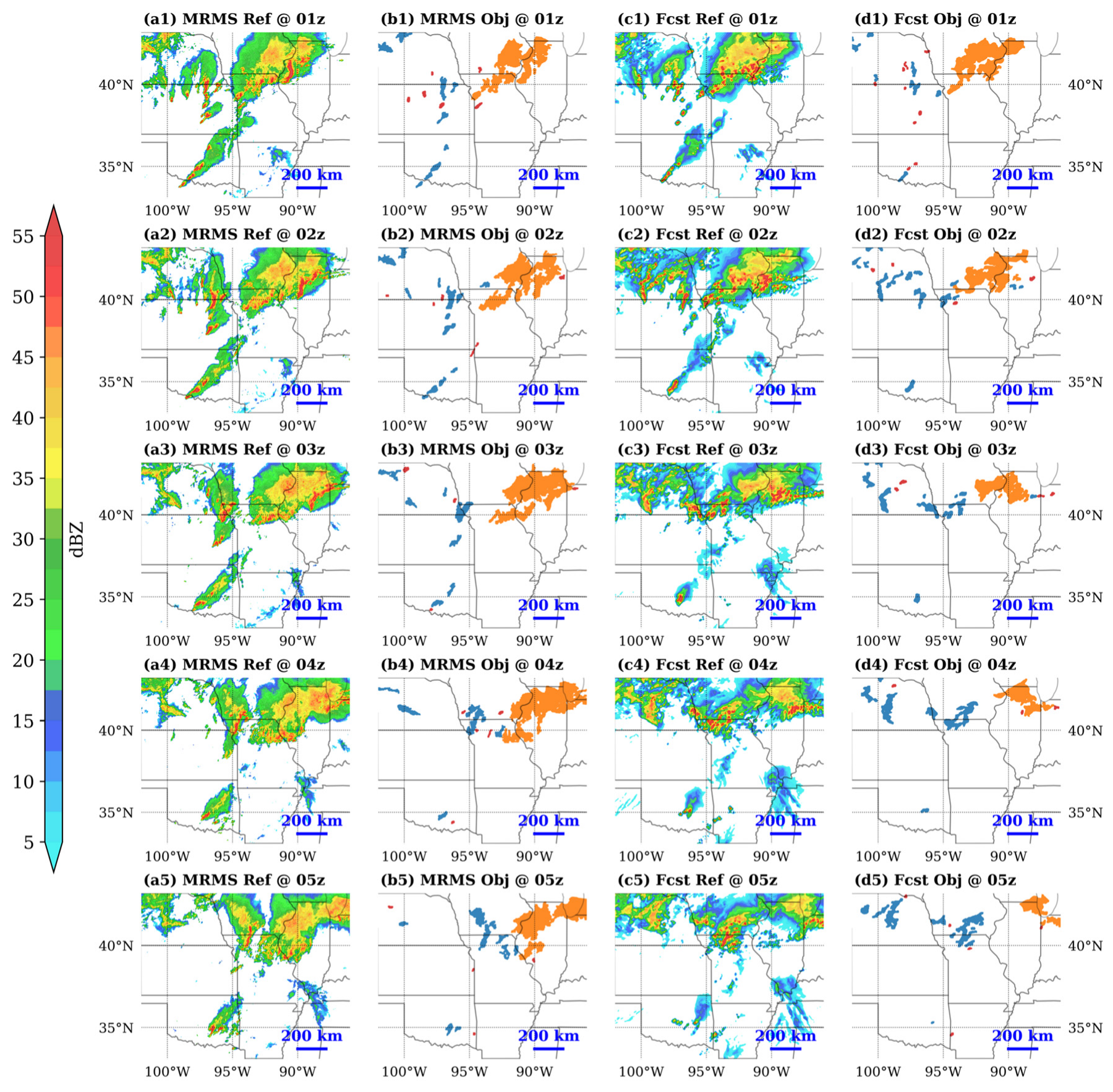
2.2. Scale-Dependent Verification of Simulated Reflectivity

Ref. [19] proposed an object-based tracking technique to identify convective storms as objects and track them over time. With the proposed technique, the space-time structure and evolution of each storm can be explicitly described by a time series of objects or an object trajectory (OT), as referred to by [19]. OT allows one to define an attribute of a storm by considering its temporal evolution.
To enable a scale-dependent evaluation of the MULTI and LARGE ensemble forecasts during the 2019 SFE, we applied the tracking technique of [19] to all reflectivity forecasts and MRMS observations. Specifically, spatial objects were first identified with a 35 dBZ threshold and then tracked over time to identify OTs. Details of the parameters used in the forecast and observed in storm tracking are described in [19]. We chose the eastern USA. (east of 105 °W) as our verification domain for object identification, tracking, and subsequent scale-dependent verification, following [32]. After OTs were identified in each 36h forecast and the corresponding MRMS observations, OT sizes were identified. We define the OT size of a storm by using the medium (50th percentile) object size within the OT, with the object size defined by the square root of its convex area. Based on the OT sizes, identified objects in each 36h forecast and the corresponding observations were classified into meso-alpha, meso-beta, and meso-gamma scales following the mesoscale subclass definitions (e.g., [33]).
To illustrate the OT-based scale classification, Figure 3 shows the observed and 1–5h forecast storm evolutions from 01z to 05z on 29 May 2019 and the corresponding identified OTs with different scales. The selected time period and subdomain featured several storms with distinct spatial scales, including a mature mesoscale convective system (MCS) to the northeast of the subdomain, a line of meso-beta scale storms from northern Texas to southern Nebraska, and several meso-gamma scale “pulse” storms that dissipated within one hour after initiation. The color-coding of the storm objects in columns b and d demonstrate that the OT method is able to reasonably identify the distinct scales of both observed and forecast storms.
After all storm objects were classified based on OT size, each observed or forecasted reflectivity field was decomposed into three mutually exclusive subfields, with each subfield including one of the three scales. A neighborhood-based verification framework was then applied. Specifically, the neighborhood maximum ensemble probability (NMEP) was calculated for the three subfields with a variety of neighborhood sizes, ranging from 3 km (model native grid) to 150 km and with two different thresholds: 35 and 45 dBZ. The NMEP was used in our study rather than the neighborhood ensemble probability (NEP) to ensure we had sufficient sample sizes for the skill comparison of scale-dependent subfields [34]. Common skill measures, such as the ractions Skill Score (FSS) and reliability diagrams, were calculated for the NMEP-based evaluation (e.g., [9]).
Figure 4 shows the NMEPs for the full fields and scale-dependent subfields of 1h MULTI and LARGE forecasts, validated for the representative case of 01z, 29 May 2019. The subfields for computing the NMEPs were derived from the OT-based object classification illustrated in Figure 3. A comparison of the full-field NMEPs of MULTI and LARGE in Figure 3a indicates that MULTI has more small-to-medium probabilities than LARGE. Although it is not immediately clear from the full-field NMEPs which ensemble is more, such a distinction demonstrates MULTI’s improved ability at sampling a multi-scale spatial uncertainty at initial forecast hours.
The scale-dependent verification at the meso-alpha scale suggests the comparable skills of MULTI and LARGE (Figure 4b,f); both ensembles simulated the location and spatial extent of the observed storm with a high accuracy. Nevertheless, the larger ensemble spread of MULTI to the south of the main storm region led to the slightly better performance of MULTI over LARGE.
For the meso-beta and gamma scales, a major distinction between the probabilistic skills of MULTI and LARGE was the prediction of the isolated storms in central Kansas, in which MULTI showed better skill on both scales. Although the full-field NMEP comparison indicated a comparable performance of the two ensembles at predicting the Kansas storms, the scale of the storms in terms of size and duration were underestimated by both ensembles (see Figure 3). As a result, the NMEPs in central Kansas were underestimated on the meso-beta scale (Figure 4c,g) and overestimated on the meso-gamma scale (Figure 4d,h), with LARGE’s under- and overestimation being more severe than the MULTI’s.
In addition to the Kansas storms, MULTI’s better performance on the meso-beta scale was also evident from the line of storms from northern Texas to southern Oklahoma. While LARGE showed too much confidence in predicting one of the storms near the border of Texas and Oklahoma, MULTI was able to sample the uncertainty and predict the coverage of the storm cluster with better skill. The subtle differences we observed in the scale-dependent NMEPs of the two ensembles demonstrated the added benefit of scale-dependent verification over the traditional approach.

3. Results and Discussion

3.1. Perturbation Characteristics for Non-Precipitation Variables

The distributions of perturbation energy across the different spatial scales for non-precipitation variables (i.e., wind and temperature) are first evaluated. Similar to JW20, the perturbation energy at different wavelengths for zonal and meridional wind and temperature at several model levels are calculated. As an example, Figure 5 shows an 850 hPa zonal wind perturbation-energy spectra and the ratio of energy between MULTI and LARGE at several forecast hours. The spectra were calculated using a two-dimensional, discrete cosine transform technique over the verification domain, averaged over ten ensemble members and 25 cases. The full spectrum covers wavelengths ranging from 6 km to approximately 2000 km with meso-alpha, meso-beta, and meso-gamma regions marked with lines and denoted by texts in each subfigure.
Similar to the findings of JW20, MULTI shows a significantly larger perturbation energy than LARGE, especially at meso-beta and gamma scales at the initial time. Such a difference is rapidly reduced over the 1–3h forecast for all scales. Consistent with JW20, MULTI’s greater perturbation energy at the 3h forecast is only evident for the meso-beta scale, with negligible differences in the meso-alpha and meso-gamma scales (Figure 5(a2)). For the 3h forecast, it is also worth noting that LARGE’s energy actually became slightly larger than MULTI’s energy for wavelengths greater than 500 km (Figure 5(b2)), a new finding since JW20 that was made possible due to the larger CONUS domain used in our study. As forecast hours increased, MULTI’s excess of meso-beta and gamma energy continued to reduce, while LARGE’s excess of meso-alpha energy continued to expand. The reduced difference between the LARGE and MULTI perturbation energies on meso-beta and meso-gamma scales with an increasing lead time is a result of the spin up of the smaller scale perturbations that are absent in the LARGE ICPs. The perturbation energy of both ensembles became comparable for the meso-gamma scale at 6h and meso-beta scale at 12h. During the second-day forecast period (18–36h), the energy differences between MULTI and LARGE on the meso-beta and gamma scales were indistinguishable, but LARGE’s excess energy on the meso-alpha scale continued (see Figure 5(a5,b5)). LARGE’s consistent meso-alpha energy surplus over MULTI at the second day is another new finding since JW20 and was made possible due to the extended forecasting period.

3.2. Simulated Reflectivity Verification

3.2.1. Ensemble Bias Characteristics

The ensemble bias is evaluated using areal coverage of grid points greater than a fixed threshold for all ensemble members and MRMS data averaged over all cases. Figure 6 shows the results for the full field- and scale-dependent subfields with 35 dBZ and 45 dBZ thresholds. The 45 dBZ threshold is used to focus on relatively strong convection, while the 35 dBZ threshold allows for weaker convection and stratiform precipitation to also be evaluated. To illustrate ensemble distributions, both the ensemble mean results and the standard deviation of the ensemble members are included in Figure 6.
The largest difference between MULTI and LARGE occurred during the first 18h. For both the 35 and 45 dBZ thresholds, the difference was characterized as an initial, (1–3h) significantly larger coverage of the meso-gamma and beta scales from MULTI, continued by a larger coverage of te meso-alpha scales from LARGE during the 3–18h period. The significant difference during the 1–3h period is a combined result of spin up by the LARGE ensemble and the spurious storms formed around observed convections in MULTI that usually die out before 3h (see Figure 4c,d). The difference between MULTI and LARGE during the second-day forecast period is much smaller with MULTI having a slightly larger coverage of meso-beta storms after 27h at the 35 dBZ threshold.
The differences between the ensembles and the observation are more substantial than the differences between MULTI and LARGE at most of the forecast lead times. Such differences include the misplaced diurnal cycle at the 35 dBZ threshold (Figure 6a) and the overestimated storm coverage throughout the forecast period at the 45 dBZ threshold (Figure 6b). A scale-dependent evaluation of MULTI and LARGE indicates that both ensembles overpredicted the meso-gamma and beta storm coverage during the 3–36h forecast period, with MULTI having an additional overprediction during the initial 1–3h (Figure 6e–h). As previously mentioned, MULTI’s overprediction of the meso-gamma and beta storm coverage over 1–3h are associated with the spurious, short-lived storms that were prone to initiate around the observed convection. Despite the overestimation for the meso-gamma and beta scale storm coverage, the timing of the peaks and valleys of the observed diurnal cycle are, in fact, well-represented by both ensembles in Figure 6e–h. The diurnal maxima of the observed coverage on the meso-alpha scale with the 35 dBZ threshold likely corresponds to the upscale growth of the mesoscale convective systems with large, stratiform precipitation regions of moderate-intensity reflectivity. The under-forecasting of the 35 dBZ diurnal cycle peaks on the meso-alpha scale (Figure 6c), and the corresponding over-forecasting of the 35 dBZ diurnal cycle peaks on smaller scales (Figure 6e,g), suggesting that the forecast model did not represent the upscale growth and the merging of broad areas of moderate reflectivity associated with stratiform precipitation areas well. Since this error is common to both MULTI and LARGE, it is likely a model or physics error rather than a direct result of the ICPs.
Unlike the systematic biases for the meso-gamma and beta scale storm coverage, the meso-alpha scale evaluation reveals distinct ensemble biases between the 35 and 45 dBZ thresholds. Specifically, both ensembles showed substantial underestimation at the 35 dBZ threshold (Figure 6c), in contrast to the consistent overestimation at the 45 dBZ threshold (Figure 6d) for meso-alpha storm coverage. The overall out-of-phase diurnal cycle at the 35 dBZ threshold (Figure 6a) is contributed to solely by the meso-alpha scale, with ensemble peaks located at approximately 27h of lead time at 03z, while observed peaks occurred at 30h of lead time at 06z.
To further investigate the distinct biases we identified in Figure 6, the number of storms present at each forecast hour is evaluated. This additional measure of ensemble bias was derived from the number of OTs identified over the verification domain. Since the scale of each storm was already identified by the OT size, the total number of storms at any forecast hour can be easily divided into the number of storms at each of the three scales we define. Figure 7 shows the total number of forecasts (MULTI and LARGE) and MRMS storms for meso-alpha, beta, and gamma scales for all 25 cases, averaged over all ensemble members at each forecast hour.
As is shown in Figure 7, both ensembles overestimated the number of meso-gamma and beta storms throughout the 36h forecast period, with MULTI having a more serious overprediction than LARGE in the initial 1–3h period. This result suggests the areal coverage overprediction in Figure 6e–h is attributable to an overpredicted number of meso-beta and gamma storms by both ensembles (see Figure 4). The number of meso-alpha storms were, in general, comparable with the verified observations, suggesting the underprediction (overprediction) of meso-alpha storm coverage at the 35 (45) dBZ thresholds was not related to the number of simulated storms.
Figure 8 shows an example of the typical ensemble biases identified for meso-alpha storms. The top row of Figure 8 presents the observed reflectivity and simulated reflectivity from the control forecast, as well as the selected MULTI and LARGE members. As is clear from the comparison, none of the simulated reflectivity fields from Figure 8b–d were able to reproduce the spatial extent of the trailing stratiform regions accompanying the observed convective systems in Figure 8a. As the intensity of the stratiform regions within an MCS or squall line is usually between 35–45 dBZ, such a weakness is reflected as an underestimation of areal coverage for meso-alpha storms only for the 35 dBZ thresholds and not for the 45 dBZ thresholds. The observed convective areas from the MCS and the squall line were actually overestimated in this example, and such overestimation explains the systematically overestimated areal coverage of meso-alpha storms at the 45 dBZ thresholds (Figure 7d). A closer examination of the MULTI and LARGE NEPs at the 45 dBZ threshold (Figure 8g,h) indicates a more severe overestimation of convective regions by LARGE than MULTI, which is consistent with the larger areal coverage biases of LARGE than MULTI during the 6–12h forecasts in Figure 7a–d.

3.2.2. Ensemble Spread Characteristics

Ensemble spread in terms of simulated reflectivity is first evaluated with correspondence ratio (CR, [35]). CR is defined as the ratio between the number of grid points in which a predetermined number of ensemble members agree that an event occurred and the number of grid points in which any ensemble member shows that the event occurred. Therefore, a smaller value of CR indicates a greater ensemble spread. An “event occurred” is defined as reflectivity that exceeds a predetermined threshold (35 dBZ in our application). The threshold number of ensemble members who agree that the event occurred can be set to any number between one and ten for a ten-member ensemble, with a larger number being a stricter application. Here, we follow [9,36] and choose a relaxed number: four out of ten members. Therefore, a CR of one (0) for one grid point indicates that at least four ensemble members (at most three ensemble members) agree on the event occurring at that location. As the value of the CR is positively (negatively) correlated with the degree of ensemble agreement (disagreement), it is often used to measure ensemble spread in non-continuous spatial variables such as reflectivity.
Figure 9 shows the distribution of the CR for the full reflectivity fields of MULTI and LARGE ensembles as well as the scale-dependent fields decomposed by the OT-based method. MULTI has a larger CR-based spread than LARGE across all scales during the initial 1–3 forecast hours, consistent with the perturbation-energy differences of the 850 hPa zonal wind in Figure 5. Also consistent with Figure 5 is the subsequent evolution of ensemble spread for the scale-dependent subfields. For example, the meso-gamma scale difference between MULTI and LARGE is minimal after 3h (Figure 9d). The ensemble spread of LARGE for meso-alpha scale storms increased more quickly and surpassed MULTI after four hours into the forecast (Figure 9b). For the meso-beta scale (Figure 9c), MULTI’s larger ensemble spread maintained for 7–8h into the forecast before LARGE caught up and became slightly more dispersive between 24h and 30h. The highly consistent CR differences between the scale-dependent reflectivity fields in Figure 9 and the perturbation-energy differences in Figure 5 are an indication of the physical rationality of the OT-based scale decomposition.
Due to the scale-dependent bias characteristics illustrated in Section 3.2.1, the ensemble spread by the CR is also diagnosed with bias-corrected ensemble members. The method for bias correction is probability matching (PM; [37]), which corrects the areal coverage bias of the ensemble forecasts by replacing the grid point value of each forecast with the corresponding observed value at the same percentile. The assumption behind PM is that the best spatial representation is provided by the forecasts, while the best Probability Density Function of magnitudes is provided by the observation. A PM-based bias correction is applied to scale-dependent subfields and combined to obtain bias-corrected full fields. The CR for the bias-corrected ensembles suggests similar patterns in terms of the relative CR positions of MULTI vs LARGE and an improved spread for both ensembles.

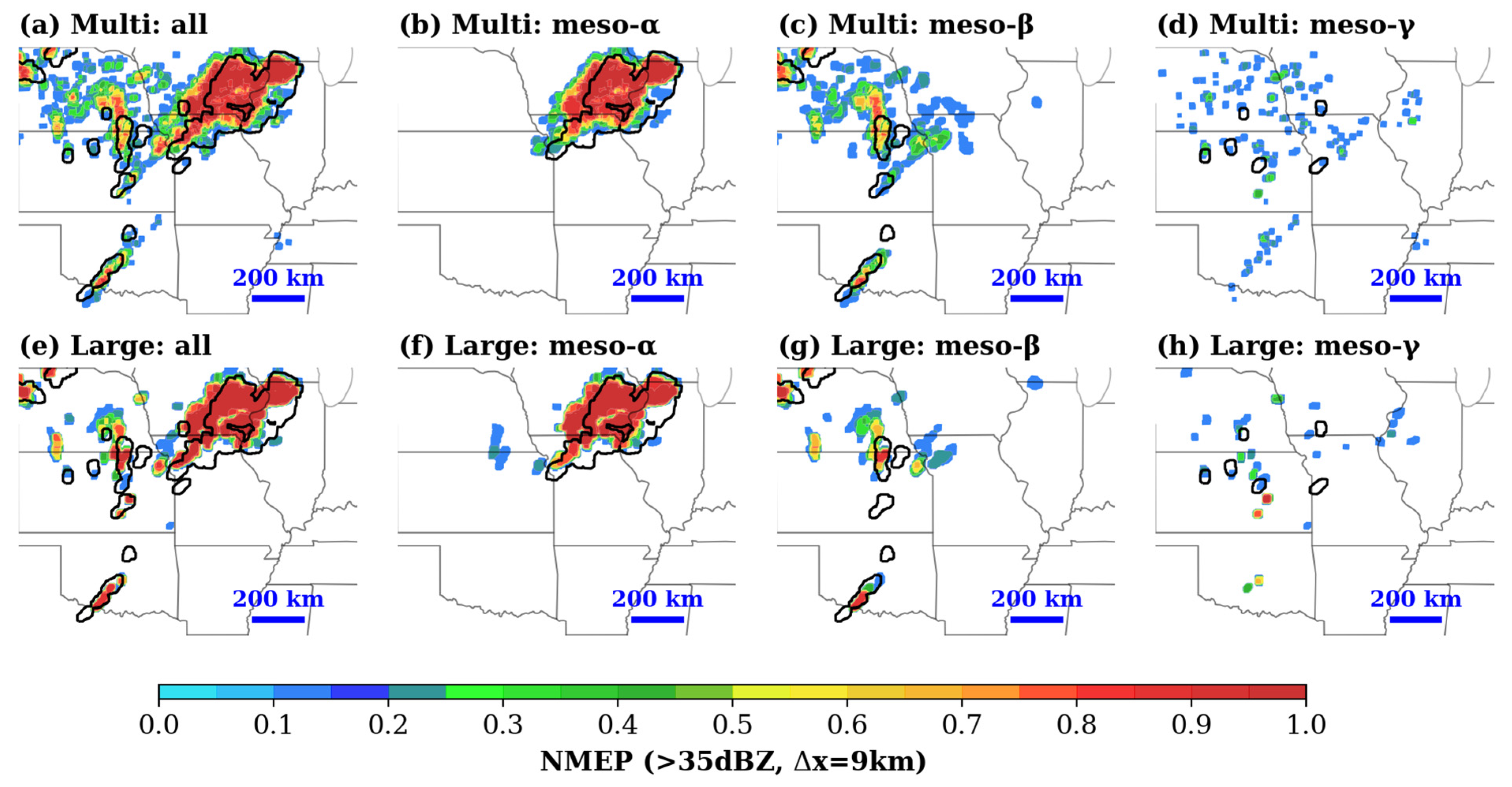
3.2.3. Neighborhood-Based Ensemble Skill

The NMEPs for a series of neighborhood sizes (3 km~150 km) and two thresholds (35 and 45 dBZ) are derived for the full fields and scale-dependent subfields of both ensembles. To understand the effect of ensemble bias on neighborhood skill, NMEP is computed for both the original ensemble forecasts and the forecasts after PM-based bias correction. The fractions skill score (FSS; [38]) was applied to these NMEPs to evaluate the overall and scale-dependent ensemble skills of MULTI and LARGE. The FSS for NMEPs obtained with different thresholds, neighborhood sizes, and whether bias correction was applied all show similar qualitative conclusions. For brevity, results are presented only for bias-corrected NMEPs of the 35 dBZ threshold and 9 km neighborhood size in Figure 10. Results with another neighborhood size, threshold, or before bias correction will be briefly discussed only if their qualitative conclusions differ from Figure 10. For reliability diagrams, we are limited to diagnostics with a 35 dBZ threshold and for the first-day forecast period; when a 45 dBZ threshold is applied or a second-day forecast period is selected, the NMEP sample sizes for medium- to large-probability bins at scale-dependent subfields become too small to conclude anything informative.
Figure 10 indicates that MULTI was significantly more skillful than LARGE during the initial 1–6h forecast period due to more skillful meso-beta and gamma-scale predictions. While the MULTI forecasts contained more small storms surrounding observed convective systems during the first three forecast hours (e.g., Figure 4a and Figure 7c), this time period corresponds to an increase, rather than a decrease, in MULTI’s probabilistic forecast skill when compared to LARGE (Figure 10a) After 6h, while the advantage still exists for meso-beta scale, MULTI’s overall advantage becomes less significant because of its slightly degraded skill on the meso-alpha scale when compared to LARGE. Figure 11 shows the dependency of a full-field FSS (Figure 11a) and a subfield FSS (Figure 11b) on neighborhood sizes at 9h of lead time. Overall, MULTI has consistently better performance, which is significant for neighborhood sizes of 30 km and greater. This overall advantage is contributed to the consistently better forecast skills of MULTI on the meso-beta and gamma skills for all neighborhood sizes. MULTI’s performance on the meso-alpha scale is also consistently worse than LARGE, but not statistically significant. Figure 11 demonstrates that the relative performance of MULTI vs LARGE is not sensitive to neighborhood sizes for both the full field and the scale-dependent FSSs.
Figure 12 shows the reliability (a–d) and sharpness (e–h) diagrams [39] for NMEPs with a 35 dBZ threshold and 9 km neighborhood size during 1–6h of the forecasts of MULTI and LARGE. The reliability diagrams indicate that MULTI has a better overall reliability for most probability bins; this is mainly due to its significantly better reliability of the meso-beta scale. The better reliability of MULTI was accompanied by less-sharp distributions, or a greater ensemble spread, with fewer NMEP counts in the high-probability bins (Figure 12e–h). MULTI is also more reliable than LARGE across all scales for small-probability bins, suggesting the greater ensemble spread of MULTI contributed to the more reliable prediction of rare events. Meso-gamma scale reliability cannot be properly examined across the full probability range due to a limited sample size of meso-gamma scale events in medium- to high-probability bins. However, for low-probability events, both ensembles showed a significant wet bias with little or no skill, suggesting there remain great challenges to make reliable predictions of these small-scale, highly localized events.
The significantly better overall reliability of MULTI continues into the 7–12h forecast period for most probability events but is less significant than the earlier forecast period (Figure 13a–d). Although there were insufficient samples to evaluate the highest forecast probabilities on the meso-beta scale, it is clear that MULTI’s advantage for medium-probability bins has continued during this 7–12h forecast range. On the meso-alpha scale, MULTI shows a degraded reliability across all probability bins, with significantly worse reliability for small- to medium-probability events (<0.5, Figure 13b). The meso-alpha scale degradation of MULTI for small- to medium-probability events is characterized by underprediction, in accordance with the distinct bias demonstrated in Section 3.2.2 and Figure 9; both MULTI and LARGE underpredict the stratiform area of meso-alpha scale systems, but LARGE also overpredicts the convective region and such a “compensation” makes it seemingly more reliable in the <0.5 probability range. MULTI also showed a slightly degraded reliability for the meso-alpha scale in large probability bins (>0.5) and contributed to the overall worse performance at the 0.9 probability bin (Figure 13a). Figure 13b indicates that both ensembles overpredict large-probability meso-alpha events, while such overprediction is more severe for MULTI.
The above diagnostics illustrate an interesting finding with respect to the relative performance of the two ensembles on the meso-alpha scale: MULTI shows slightly degraded performance during the 6–12h period and a significantly improved performance during the 20–24h period, despite having a smaller ensemble spread than LARGE during both periods. This suggests that a larger ensemble spread may not always lead to more properly sampled uncertainty and an improved skill. To better understand the relative performances of the two ensembles on the meso-alpha scale during the second-day forecast period, Figure 14 shows the NMEPs of the 27h MULTI and LARGE forecasts valid at 03z; 29 May 2019, derived from the full fields and scale-dependent subfields with 35 dBZ thresholds and a 9 km neighborhood size. Compared to the NMEPs of the 1h forecasts in Figure 4; a notable difference in the probability fields is evident at the meso-beta and gamma scales: unlike the highly confident prediction in Figure 4; the high probability events of both ensembles are greatly reduced in the meso-beta and gamma NMEP fields at the 27h lead time. All of the large probability values (>0.7) are associated with the prediction of the meso-alpha scale storm to the northeast of the subdomain (Figure 14b,f), and MULTI shows a noticeably more skillful prediction than LARGE for this storm.

4. Conclusions

Since convection-allowing ensemble forecast systems have become increasingly utilized in operational forecast settings, there has been an increasing interest in understanding optimal methods of generating initial condition perturbations for such ensembles. Downscaling perturbations from a coarser resolution ensemble (i.e., LARGE) provides a cost-effective solution for initializing the convection-allowing ensemble. However, initial studies have suggested that the expense of a convective-scale data assimilation system to provide realistic convective scale perturbations (i.e., MULTI) can have further advantages, especially over limited forecast domains and on relatively short forecast lead times. This study builds on these initial studies by evaluating the multi-scale performance of both types of initial condition perturbations in a CONUS-domain ensemble out to the 36-h forecast lead time. This study leverages a novel approach to the scale-dependent verification based on the tracking of forecast objects across time.
The evaluation of non-precipitation variables revealed that MULTI provided more perturbation energy than LARGE on meso-beta and meso-gamma scales at early lead times, but less perturbation energy on meso-alpha scales. The lower perturbation energy on the largest scales was not seen in earlier studies, which used a smaller forecast domain. After the 18h lead time, which was the latest forecast time considered in JW20, the perturbation energy is indistinguishable between MULTI and LARGE on meso-gamma and meso-beta scales. However, the increased perturbation energy for LARGE on the meso-alpha scales persists into the day-two forecast. In terms of reflectivity, MULTI had more ensemble spread than LARGE at early forecast hours on all spatial scales, while LARGE had more spread than MULTI after ~8h on the the meso-alpha scale.
The different IC perturbation methods were found to affect the ensemble bias of simulated reflectivity forecasts. In particular, the areal coverage of meso-gamma and meso-beta scale objects was over-forecast by MULTI during the first three forecast hours. From approximately 3 to 24h, MULTI then had less coverage of meso-alpha-scale objects than LARGE. After 24h, MULTI had more over-forecasting than LARGE for meso-beta-scale objects for both 35 and 45 dBZ thresholds.
The overall probabilistic forecast skill, after bias correction with probability matching, was evaluated for both ensembles using the neighborhood maximum ensemble probability. A significant advantage of MULTI over LARGE in terms of the NMEP skill was found in the first six forecast hours using a 9 km neighborhood radius. For 9–12h forecasts, a MULTI advantage on the meso-gamma and meso-beta scales outweighed a LARGE advantage on meso-alpha scales across a range of neighborhood radii. At the 24-h lead time, MULTI had an advantage over LARGE for meso-alpha objects only when verified with small neighborhood radii, suggesting that the small-scale IC perturbations help to improve the forecast of convective-scale details of large convective systems, even at the one-day lead time. However, the meso-beta objects are more skillfully forecast with LARGE at this lead time when verified with larger neighborhood radii, suggesting an improved probabilistic forecast of the approximate locations and intensity of meso-beta-scale objects in LARGE at longer forecast ranges.
In general, we can conclude that neither MULTI nor LARGE is unequivocally better across the range of forecast lead times, spatial scales, and neighborhood radii considered. MULTI has the advantage of improving probabilistic forecasts of convective-scale details and short lead-time forecasts, while LARGE has the advantage of a greater large-scale spread and a better skill of approximate locations and intensities of mesoscale objects at an ~1 day lead time. It is therefore likely that the optimal initial-condition perturbation method for large-domain, convection-allowing ensemble forecasts used for both short- and long-range forecasts should include some combination of the MULTI and LARGE IC perturbation techniques. Future work will further evaluate the impact of blending the CAE analysis perturbations with downscaled, global model perturbations, including longer lead times of 2–3 days. Future work may also consider whether the inclusion of additional observation, such as high resolution satellite radiances, affect the relative performance of MULTI and LARGE.
While this study suggests advantages of MULTI primarily for lead times of up to approximately 6h and advantages of LARGE primarily for lead times of ~1 day, it should be considered that the focus of this evaluation was on forecasts of springtime, midlatitude convection. Given the different dynamics and physics that dominate in other seasons and other regions (e.g., the tropics or the Arctic) the results may not be generally applicable to all forecast applications.

Author Contributions

Conceptualization, A.J., F.H., Y.W. and X.W.; methodology, A.J., F.H., Y.W. and X.W.; software, Y.W.; validation, F.H. and Y.W.; formal analysis, A.J. and F.H.; investigation, A.J. and X.W.; resources, X.W.; data curation, F.H. and Y.W.; writing—original draft preparation, A.J., F.H. and Y.W.; writing—review and editing, A.J. and X.W.; visualization, A.J. and F.H.; supervision, X.W.; project administration, X.W.; funding acquisition, X.W. All authors have read and agreed to the published version of the manuscript.

Funding

This research was funded by the NOAA Awards NA17OAR4590116 and NA22OAR4590532.

Data Availability Statement

All experiments evaluated in this study can be replicated following the methods described above, using the GEFS, GFS, SREF data available, as cited in [40,41,42], and the WRF and GSI-EnVAR software, as cited in [43,44]. The forecast products produced during this study are also archived locally and can be made available upon request to the authors.

Acknowledgments

The forecast ensembles verified in this study were generated using the Stampede2 machine at Extreme Science and Engineering Discovery Environment (XSEDE), which is supported by the National Science Foundation Grant ACI-1053575. Post-processing and verification also utilized resources provided by the University of Oklahoma (OU) Supercomputing Center for Education and Re-search (OSCER).

Conflicts of Interest

The authors declare no conflict of interest. The funders had no role in the design of the study; in the collection, analyses, or interpretation of data; in the writing of the manuscript; or in the decision to publish the results.

References

  1. Weisman, M.L.; Davis, C.; Wang, W.; Manning, K.W.; Klemp, J.B. Experiences with 0–36-h Explicit Convective Forecasts with the WRF-ARW Model. Weather Forecast. 2008, 23, 407–437. [Google Scholar] [CrossRef]
  2. Johnson, A.; Wang, X.; Xue, M.; Kong, F. Hierarchical Cluster Analysis of a Convection-Allowing Ensemble during the Hazardous Weather Testbed 2009 Spring Experiment. Part II: Ensemble Clustering over the Whole Experiment Period. Mon. Weather. Rev. 2011, 139, 3694–3710. [Google Scholar] [CrossRef] [Green Version]
  3. Bentzien, S.; Friederichs, P. Generating and Calibrating Probabilistic Quantitative Precipitation Forecasts from the High-Resolution NWP Model COSMO-DE. Weather. Forecast. 2012, 27, 988–1002. [Google Scholar] [CrossRef]
  4. Tennant, W. Improving initial condition perturbations for MOGREPS-UK. Q. J. R. Meteorol. Soc. 2015, 141, 2324–2336. [Google Scholar] [CrossRef]
  5. Schwartz, C.S.; Romine, G.S.; Sobash, R.A.; Fossell, K.R.; Weisman, M.L. NCAR’s Experimental Real-Time Convection-Allowing Ensemble Prediction System. Weather Forecast. 2015, 30, 1645–1654. [Google Scholar] [CrossRef]
  6. Potvin, C.K.; Carley, J.; Clark, A.J.; Wicker, L.J.; Skinner, P.; Reinhart, A.E.; Gallo, B.T.; Kain, J.S.; Romine, G.S.; Aligo, E.A.; et al. Systematic Comparison of Convection-Allowing Models during the 2017 NOAA HWT Spring Forecasting Experiment. Weather Forecast. 2019, 34, 1395–1416. [Google Scholar] [CrossRef]
  7. Johnson, A.; Wang, X.; Wang, Y.; Reinhart, A.; Clark, A.J.; Jirak, I.L. Neighborhood- and Object-Based Probabilistic Verification of the OU MAP Ensemble Forecasts during 2017 and 2018 Hazardous Weather Testbeds. Weather Forecast. 2020, 35, 169–191. [Google Scholar] [CrossRef]
  8. Roberts, B.; Gallo, B.T.; Jirak, I.L.; Clark, A.J.; Dowell, D.C.; Wang, X.; Wang, Y. What Does a Convection-Allowing Ensemble of Opportunity Buy Us in Forecasting Thunderstorms? Weather Forecast. 2020, 35, 2293–2316. [Google Scholar] [CrossRef]
  9. Gasperoni, N.A.; Wang, X.; Wang, Y. A Comparison of Methods to Sample Model Errors for Convection-Allowing Ensemble Forecasts in the Setting of Multiscale Initial Conditions Produced by the GSI-Based EnVar Assimilation System. Mon. Weather. Rev. 2020, 148, 1177–1203. [Google Scholar] [CrossRef]
  10. Gasperoni, N.A.; Wang, X.; Wang, Y. Using a Cost-Effective Approach to Increase Background Ensemble Member Size within the GSI-Based EnVar System for Improved Radar Analyses and Forecasts of Convective Systems. Mon. Weather. Rev. 2022, 150, 667–689. [Google Scholar] [CrossRef]
  11. Peralta, C.; Ben Bouallègue, Z.; Theis, S.E.; Gebhardt, C.; Buchhold, M. Accounting for initial condition uncertainties in COSMO-DE-EPS. J. Geophys. Res. Atmos. 2012, 117, D7. [Google Scholar] [CrossRef]
  12. Kühnlein, C.; Keil, C.; Craig, G.C.; Gebhardt, C. The impact of downscaled initial condition perturbations on convective-scale ensemble forecasts of precipitation. Q. J. R. Meteorol. Soc. 2013, 140, 1552–1562. [Google Scholar] [CrossRef]
  13. Schwartz, C.S.; Romine, G.S.; Smith, K.R.; Weisman, M.L. Characterizing and Optimizing Precipitation Forecasts from a Convection-Permitting Ensemble Initialized by a Mesoscale Ensemble Kalman Filter. Weather Forecast. 2014, 29, 1295–1318. [Google Scholar] [CrossRef] [Green Version]
  14. Johnson, A.; Wang, X. Interactions between Physics Diversity and Multiscale Initial Condition Perturbations for Storm-Scale Ensemble Forecasting. Mon. Weather. Rev. 2020, 148, 3549–3565. [Google Scholar] [CrossRef]
  15. Kalina, E.A.; Jankov, I.; Alcott, T.; Olson, J.; Beck, J.; Berner, J.; Dowell, D.; Alexander, C. A Progress Report on the Development of the High-Resolution Rapid Refresh Ensemble. Weather Forecast. 2021, 36, 791–804. [Google Scholar] [CrossRef]
  16. Johnson, A.; Wang, X. A Study of Multiscale Initial Condition Perturbation Methods for Convection-Permitting Ensemble Forecasts. Mon. Weather. Rev. 2016, 144, 2579–2604. [Google Scholar] [CrossRef]
  17. Wang, Y.; Wang, X. Development of Convective-Scale Static Background Error Covariance within GSI-Based Hybrid EnVar System for Direct Radar Reflectivity Data Assimilation. Mon. Weather. Rev. 2021, 149, 2713–2736. [Google Scholar] [CrossRef]
  18. Wang, Y.; Wang, X. Direct Assimilation of Radar Reflectivity without Tangent Linear and Adjoint of the Nonlinear Observation Operator in the GSI-Based EnVar System: Methodology and Experiment with the 8 May 2003 Oklahoma City Tornadic Supercell. Mon. Weather Rev. 2017, 145, 1447–1471. [Google Scholar] [CrossRef]
  19. Han, F.; Wang, X. An Object-Based Method for Tracking Convective Storms in Convection Allowing Models. Atmosphere 2021, 12, 1535. [Google Scholar] [CrossRef]
  20. Smith, T.M.; Lakshmanan, V.; Stumpf, G.J.; Ortega, K.; Hondl, K.; Cooper, K.; Calhoun, K.; Kingfield, D.; Manross, K.L.; Toomey, R.; et al. Multi-Radar Multi-Sensor (MRMS) Severe Weather and Aviation Products: Initial Operating Capabilities. Bull. Am. Meteorol. Soc. 2016, 97, 1617–1630. [Google Scholar] [CrossRef]
  21. Skamarock, W.C.; Klemp, J.B.; Dudhia, J.; Gill, D.O.; Barker, D.M.; Duda, M.G.; Huang, X.-Y.; Wang, W.; Powers, J.G. A Description of the Advanced Research WRF Version 3; NCAR Technical Note NCAR/TN-475+STR; NCAR: Boulder, CO, USA, 2008; 113p. [Google Scholar] [CrossRef]
  22. Johnson, A.; Wang, X.; Carley, J.; Wicker, L.J.; Karstens, C. A Comparison of Multiscale GSI-Based EnKF and 3DVar Data Assimilation Using Radar and Conventional Observations for Midlatitude Convective-Scale Precipitation Forecasts. Mon. Weather. Rev. 2015, 143, 3087–3108. [Google Scholar] [CrossRef]
  23. Whitaker, J.S.; Hamill, T.M. Ensemble Data Assimilation without Perturbed Observations. Mon. Weather Rev. 2002, 130, 1913–1924. [Google Scholar] [CrossRef]
  24. Wang, X. Incorporating Ensemble Covariance in the Gridpoint Statistical Interpolation Variational Minimization: A Mathematical Framework. Mon. Weather Rev. 2010, 138, 2990–2995. [Google Scholar] [CrossRef] [Green Version]
  25. Wang, X.; Parrish, D.; Kleist, D.T.; Whitaker, J.S. GSI 3DVar-Based Ensemble–Variational Hybrid Data Assimilation for NCEP Global Forecast System: Single-Resolution Experiments. Mon. Weather Rev. 2013, 141, 4098–4117. [Google Scholar] [CrossRef]
  26. Wang, Y.; Wang, X. Rapid Update with EnVar Direct Radar Reflectivity Data Assimilation for the NOAA Regional Convection-Allowing NMMB Model over the CONUS: System Description and Initial Experiment Results. Atmosphere 2021, 12, 1286. [Google Scholar] [CrossRef]
  27. Whitaker, J.S.; Hamill, T.M. Evaluating Methods to Account for System Errors in Ensemble Data Assimilation. Mon. Weather Rev. 2012, 140, 3078–3089. [Google Scholar] [CrossRef]
  28. Nakanishi, M.; Niino, H. Development of an Improved Turbulence Closure Model for the Atmospheric Boundary Layer. J. Meteorol. Soc. Jpn. Ser. II 2009, 87, 895–912. [Google Scholar] [CrossRef] [Green Version]
  29. Thompson, G.; Field, P.R.; Rasmussen, R.M.; Hall, W.D. Explicit Forecasts of Winter Precipitation Using an Improved Bulk Microphysics Scheme. Part II: Implementation of a New Snow Parameterization. Mon. Weather Rev. 2008, 136, 5095–5115. [Google Scholar] [CrossRef]
  30. Smirnova, T.G.; Brown, J.M.; Benjamin, S.G.; Kenyon, J.S. Modifications to the Rapid Update Cycle Land Surface Model (RUC LSM) Available in the Weather Research and Forecasting (WRF) Model. Mon. Weather. Rev. 2016, 144, 1851–1865. [Google Scholar] [CrossRef]
  31. Mlawer, E.J.; Taubman, S.J.; Brown, P.D.; Iacono, M.J.; Clough, S.A. Radiative transfer for inhomogeneous atmospheres: RRTM, a validated correlated-k model for the longwave. J. Geophys. Res. Atmos. 1997, 102, 16663–16682. [Google Scholar] [CrossRef] [Green Version]
  32. Duda, J.D.; Wang, X.; Wang, Y.; Carley, J.R. Comparing the Assimilation of Radar Reflectivity Using the Direct GSI-Based Ensemble–Variational (EnVar) and Indirect Cloud Analysis Methods in Convection-Allowing Forecasts over the Continental United States. Mon. Weather Rev. 2019, 147, 1655–1678. [Google Scholar] [CrossRef]
  33. Wilkins, A.; Johnson, A.; Wang, X.; Gasperoni, N.A.; Wang, Y. Multi-Scale Object-Based Probabilistic Forecast Evaluation of WRF-Based CAM Ensemble Configurations. Atmosphere 2021, 12, 1630. [Google Scholar] [CrossRef]
  34. Schwartz, C.S.; Sobash, R.A. Generating Probabilistic Forecasts from Convection-Allowing Ensembles Using Neighborhood Approaches: A Review and Recommendations. Mon. Weather Rev. 2017, 145, 3397–3418. [Google Scholar] [CrossRef]
  35. Stensrud, D.J.; Wandishin, M.S. The Correspondence Ratio in Forecast Evaluation. Weather Forecast. 2000, 15, 593–602. [Google Scholar] [CrossRef]
  36. Johnson, A.; Wang, X. Design and Implementation of a GSI-Based Convection-Allowing Ensemble Data Assimilation and Forecast System for the PECAN Field Experiment. Part I: Optimal Configurations for Nocturnal Convection Prediction Using Retrospective Cases. Weather Forecast. 2017, 32, 289–315. [Google Scholar] [CrossRef]
  37. Clark, A.J.; Gallus, W.A.; Xue, M.; Kong, F. A Comparison of Precipitation Forecast Skill between Small Convection-Allowing and Large Convection-Parameterizing Ensembles. Weather Forecast. 2009, 24, 1121–1140. [Google Scholar] [CrossRef] [Green Version]
  38. Roberts, N.M.; Lean, H.W. Scale-Selective Verification of Rainfall Accumulations from High-Resolution Forecasts of Convective Events. Mon. Weather. Rev. 2008, 136, 78–97. [Google Scholar] [CrossRef]
  39. Wilks, D.S. Statistical Methods in the Atmospheric Sciences, 3rd ed.; Elsevier: Amsterdam, The Netherlands, 2011; 676p. [Google Scholar]
  40. GEFS. Global Ensemble Forecast System Operational Forecast Files. 2019. Available online: https://registry.opendata.aws/noaa-gefs/ (accessed on 1 May 2019).
  41. GFS. Global Forecast System Operational Forecast Files. 2019. Available online: https://registry.opendata.aws/noaa-gfs-bdp-pds/ (accessed on 1 May 2019).
  42. SREF. Short Range Ensemble Forecast Operational Forecast Files. Available online: https://www.nco.ncep.noaa.gov/pmb/products/sref/ (accessed on 1 May 2019).
  43. GSI-EnVAR. Gridpoint Statistical Interpolation—Ensemble Variational Data Asssimilation Package, Version 12.0.2. 2019. Available online: https://github.com/NOAA-EMC/GSI (accessed on 15 January 2019).
  44. WRF. Weather Research and Forecast (WRF) Advanced Research WRF Version 3.9.1.1. 2019. Available online: https://github.com/NCAR/WRFV3/releases (accessed on 15 January 2019).
Figure 1. Flowchart for the EDA system at a particular DA cycle, t. The green box indicates the assimilation of conventional observations, and the red box includes the assimilation of radar-reflectivity observations. See text for details.
Atmosphere 14 00255 g001
Figure 2. The model domain for the EDA system. The E-W scale of the domain is ~4860 km, the N-S scale of the domain is ~3360 km, and latitude/longitude dashed lines are overlaid for reference.
Atmosphere 14 00255 g002
Figure 3. Hourly snapshots of (a1a5) MRMS composite reflectivity, (b1b5) objects identified, (c1c5) MAP 1–5h control forecast reflectivity, and (d1d5) objects identified from 01z to 05z, 29 May 2019. The objects in (b) and (d) are color-coded by the scale they were classified into based on the OT method: orange denotes meso-alpha storms while blue and red are for meso-beta and meso-gamma storms, respectively.
Atmosphere 14 00255 g003
Figure 4. NMEPs for the 1h forecasts of (a,e) the full field without scale separation, (b,f) meso-alpha, (c,g) meso-beta, and (d,h) meso-gamma subfields of the MULTI and LARGE ensembles. The forecasts were initialized at 00z, 29 May 2019. The NMEPs were derived with a 35 dBZ threshold and a 9 km neighborhood size. The black contours in each subfigure denote the binary neighborhood probability (BNP, [34]) of the MRMS reflectivity for the full field (in a,e) and scale-dependent subfields (in bd, fh) with the same 35 dBZ threshold and 9 km neighborhood size.
Atmosphere 14 00255 g004
Figure 5. (a1a5) Perturbation-energy spectra of MULTI (solid) and LARGE (dashed) and (b1b5) the ratio of perturbation-energy spectra between MULTI and LARGE for an 850 hPa zonal wind averaged over 25 forecast cases at analysis times for 3h, 6h, 12h, and 24h forecasts, respectively. The full wavelength range was divided into meso-alpha, meso-beta, and meso-gamma scales as marked by blue dashed lines and texts near the bottom of each subfigure.
Atmosphere 14 00255 g005
Figure 6. Forecast and MRMS areal coverage (%) over the verification domain for (first row) the full field, (2nd–4th row) meso-alpha, meso-beta, and meso-gamma subfields averaged over 25 cases with a 35 dBZ threshold (a,c,e,g) and a 45 dBZ threshold (b,d,f,h). Blue and orange dotted lines represent ensemble mean areal coverage for MULTI and LARGE, respectively, with shades representing one standard deviation range among ensemble members.
Atmosphere 14 00255 g006
Figure 7. Total number of forecasts and observed storms present at each forecast hour for (a) meso-alpha, (b) meso-beta, and (c) meso-gamma scales for all 25 cases. Blue and orange dotted lines represent ensemble mean storm counts for MULTI and LARGE, respectively, with shades representing one standard deviation range among ensemble members.
Atmosphere 14 00255 g007
Figure 8. Reflectivity for selected subdomain for (a) MRMS, (b) 9h control forecast, (c) selected MULTI member, and (d) selected LARGE member, as well as NEPs for (e) MULTI with 35 dBZ threshold, (f) LARGE with 35 dBZ threshold, (g) MULTI with 45 dBZ threshold, and (h) LARGE with 45 dBZ thresholds valid at 09z, 24 May 2019. All NEPs were derived with a neighborhood size of 9 km.
Atmosphere 14 00255 g008
Figure 9. Distributions of correspondence ratio (CR) of MULTI (solid) and LARGE (dashed) for (a) the full field, (bd) meso-alpha, meso-beta, and meso-gamma subfields aggregated over 25 cases. The inset within each subfigure highlights the CR distributions for the first 6h forecasts.
Atmosphere 14 00255 g009
Figure 10. MULTI and LARGE FSSs for NMEPs derived with a 35 dBZ threshold and a 9 km neighborhood size for (a) the full field, (b) meso-alpha, meso-beta, and meso-gamma subfields aggregated over 25 cases. Dots along the FSS curves indicate statistically significant differences determined by Wilcoxon rank sum test, with filled (open) dots representing improved (degraded) skill for MULTI at the 10% confidence level.
Atmosphere 14 00255 g010
Figure 11. FSS as a function of neighborhood sizes for NMEPs derived with the 35 dBZ threshold for (a) the full field and (b) meso-alpha, meso-beta, and meso-gamma subfields of 9h forecasts aggregated over 25 cases. Dots along the FSS curves indicate statistically significant differences determined by Wilcoxon rank sum test, with filled (open) dots representing improved (degraded) skill for MULTI at the 10% confidence level.
Atmosphere 14 00255 g011
Figure 12. (ad) Reliability diagrams and (eh) associated sharpness diagrams for the full field, meso-alpha, meso-beta, and meso-gamma subfields, respectively, accumulated over 1–6h forecasts of 25 cases. Dots (triangles) indicate statistically significant differences between MULTI and LARGE at the 10% (20%) confidence level determined by the Wilcoxon rank sum test. The dashed line in each sharpness diagram indicates the minimum sample size (100) used for presenting reliability diagram values.
Atmosphere 14 00255 g012
Figure 13. As in Figure 12, but for 7–12h forecasts (ah).
Atmosphere 14 00255 g013
Figure 14. NMEPs with 35 dBZ thresholds and neighborhood sizes of 9 km for the full field (a,e), meso-alpha (b,f), meso-beta (c,g), and meso-gamma (d,h) subfields of MULTI and LARGE for 27h forecasts valid at 03z, 29 May 2019. The black contours in each subfigure mark areas of MRMS reflectivity greater than 35 dBZ for the respectively full field (in a,d) and scale-dependent subfields (in bd, fh).
Atmosphere 14 00255 g014
Disclaimer/Publisher’s Note: The statements, opinions and data contained in all publications are solely those of the individual author(s) and contributor(s) and not of MDPI and/or the editor(s). MDPI and/or the editor(s) disclaim responsibility for any injury to people or property resulting from any ideas, methods, instructions or products referred to in the content.

