
Classification Analysis of Southwest Pacific Tropical Cyclone Intensity Changes Prior to Landfall


1
Computational Physics and Methods (CCS-2), Los Alamos National Laboratory, Los Alamos, NM 87545, USA
2
Department of Geography and Anthropology, Louisiana State University, Baton Rouge, LA 70803, USA
3
Department of Earth, Atmosphere, and Environment, Northern Illinois University, Dekalb, IL 60115, USA
*
Author to whom correspondence should be addressed.
Atmosphere 2023, 14(2), 253; https://doi.org/10.3390/atmos14020253
Submission received: 2 December 2022
/
Revised: 22 January 2023
/
Accepted: 23 January 2023
/
Published: 28 January 2023
(This article belongs to the Special Issue Tropical Cyclone Forecasting - Analysis and Methods)
Abstract
:This study evaluates the ability of a random forest classifier to identify tropical cyclone (TC) intensification or weakening prior to landfall over the western region of the Southwest Pacific Ocean (SWPO) basin. For both Australia mainland and SWPO island cases, when a TC first crosses land after spending ≥24 h over the ocean, the closest hour prior to the intersection is considered as the landfall hour. If the maximum wind speed (Vmax) at the landfall hour increased or remained the same from the 24-h mark prior to landfall, the TC is labeled as intensifying and if the Vmax at the landfall hour decreases, the TC is labeled as weakening. Geophysical and aerosol variables closest to the 24 h before landfall hour were collected for each sample. The random forest model with leave-one-out cross validation and the random oversampling example technique was identified as the best-performing classifier for both mainland and island cases. The model identified longitude, initial intensity, and sea skin temperature as the most important variables for the mainland and island landfall classification decisions. Incorrectly classified cases from the test data were analyzed by sorting the cases by their initial intensity hour, landfall hour, monthly distribution, and 24-h intensity changes. TC intensity changes near land strongly impact coastal preparations such as wind damage and flood damage mitigations; hence, this study will contribute to improve identifying and prioritizing prediction of important variables contributing to TC intensity change before landfall.
1. Introduction
Tropical cyclones (TCs) that originate over the western region of the Southwest Pacific Ocean (5° S–40° S, 135° E–180° E) can devastate the north and northeast coasts of Australia, New Zealand, and the islands of Melanesia (including Vanuatu, New Caledonia, and Fiji). The region from the northern territory to southeast Queensland is the most developed, urbanized, and populated area of Australia, making this region extremely vulnerable to the impacts of extreme TC wind speeds. TCs are an annual threat to northeastern Australia [1]. The threat is exacerbated in the far northeastern region of Australia because of the complex terrain’s proximity to the coastline, increasing the destructive potential of landfalling TCs [2]. Western Southwest Pacific Ocean (SWPO) islands such as Vanuatu, Fiji, and Solomon are also vulnerable to TC landfalls [3] because of the unfavorable shoreline to land area ratio [4] and combination of low-lying coral atolls, reef islands and volcanically composed islands [5]. The western SWPO islands also contain a large proportion of the world’s biodiversity. Intense landfalling TCs with higher intensity in a changing climate pose a threat to these natural and human habitats and the situation becomes worse because of the limited amount of financial security, mitigation and adaptation strategies [6].
TCs’ changing intensity prior to landfall and their linkage with large-scale geophysical parameters have attracted the attention of meteorologists and climatologists [7,8]. Coastal safety predominantly depends on accurate TC intensity prediction in the short window just prior to landfall, so coastal communities have enough time to start evacuation procedures. The changing intensity prior to landfall depends on the environmental condition [9,10], bathymetric characteristics of the ocean floor [11], changes in ocean temperature [12,13], terrain characteristics of the coast [14], etc. The surrounding environment of a TC making landfall somewhere along the northeast Australian coast will be different from the surrounding environment of a TC making landfall somewhere along the nearby SWPO islands, due to different large-scale environments, including different sea surface temperature (SST) conditions, sea level pressures [15,16], teleconnection patterns such as El Niño–Southern Oscillation (ENSO), as ENSO causes a shift in SST towards the west during La Niña years and towards the east during El Niño years [17], and topographic effects [18]. These differences lead to difficulties in accurately predicting the intensity change prior to landfall in computer models.
Threats associated with an approaching TC toward land are partially a function of its wind speed [8]. However, accurately predicting TC intensity has been more difficult than TC tracks in recent decades [19]. Rappaport, Franklin [8] highlighted this disparity by mentioning the need for accurately predicting TC intensity, specifically the intensification and weakening before landfall. Research on the changes in wind speed or minimum central pressure has been primarily focused on the degradation of TCs after making landfall [16,20,21]. Comparatively, few studies have emphasized TC intensification and weakening before making landfall [8,19,22]. There are several mechanisms that have been hypothesized to influence TC intensity near land that could be relevant to TC intensity during the final day or hours before landfall. Wu [23] suggested heat and moisture fluxes over land differ from that over water and the extent of their influence depends on the amount of time a storm spends over the ocean and over land. Entrainment of dry, continental air is also identified as a determining factor of TC intensity before landfall [21,24].
Atmospheric aerosols substantially influence the spatial distribution of cloudiness and hydrometeor contents that ultimately impact the wind speed of a TC approaching land. Khain, Lynn [25] found continental aerosols invigorated convection mainly toward the periphery of Hurricane Katrina in 2005. This led to weakening prior to landfall. The largest decline in winds took place approximately 24 h before landfall, just after Hurricane Katrina reached maximum intensity. Increasing aerosol intrusion into the rainband region weakens TCs [26]. Dry air that contains atmospheric aerosols can negatively impact TCs [27] by fostering enhanced cold downdrafts [28,29] and lowering the convective available potential energy within a TC [30]. According to ref. [24], dry air intrusion into a moist storm envelope weakens landfalling TCs by reducing surface moisture fluxes and increasing surface friction. The surface energy supply to the TC becomes insufficient to counteract the negative effects from enhanced dry air entrainment. Gulf Coast landfalling Hurricanes Opal (1995), Lili (2002), and Ivan (2004) weakened before their centers crossed the coastline as the eyewall convection started weakening, owing to dry air intrusion [31].
The depth of the ocean mixed layer is a considerable factor in TC intensity, as the shallow depth of the mixed layer helps storms upwell sub-surface cold water, causing the weakening of the storm [32]. Shallow coastal water also creates room for storms to upwell cool water to the surface. This negative feedback causes the storm to hinder its own increasing intensity [32,33], and this factor reveals the importance of ocean heat content (OHC) in changing TC intensity before making landfall.
There are several other ocean and atmospheric processes that modify the intensity of a storm approaching land. Steep coastal orography leads to increases in the storm intensity and associated damages over the northeastern coast of Australia [1]. TCs that approach land during neap tides (when the tides are the smallest in a location) tend to be less intense than those arriving at other times [19].
TC intensity changes prior to landfall have been emphasized in previous studies using observational and statistical analysis [8,19,22,34], high-resolution numerical simulations [15,30,31], and satellite image analyses [35,36]. Statistical models’ success is based on maintaining certain assumptions and they are susceptible to multicollinearity. Machine learning models do not violate multicollinearity assumptions, hence the model performance did not get affected by the presence of multicollinearity. Decision trees have been used to classify 24-h intensity changes [36] over the North Pacific. Geng, Shi [37] used a finite mixture model-based cluster algorithm to classify landfalling TCs over China’s coast. For TC track prediction, ref. [38] used a deep learning framework with a bidirectional gate recurrent unit network that outperforms other state-of-the-art deep learning models, including a recurrent neural network, long short-term memory neural network, and gate recurrent unit network. A deep learning-based multilayer perceptron TC intensity prediction model that used the global Statistical Hurricane Intensity Prediction Scheme predictors correctly predicted more rapid intensification events [39]. A 3D convolutional neural network (3D-CNN), along with image processing, significantly improved the mean absolute error of TC intensity change predictions and the accuracy of TC intensifying or weakening classification [40]. By using a CNN structure and geostationary satellite Himawari-8 cloud products, ref. [41] reported that the model is conducive to estimating TC intensity. A neural network framework for TC intensity prediction named TC-Pred, along with a novel feature extraction and aggregation approach, was designed by [42] and considered the characteristics of multi-source environmental variables. Their results indicate that TC-pred outperforms other machine learning models at 6 h, 12 h, 18 h, and 24 h intervals, respectively. However, studies on the use of machine learning applications to classify TC intensification or weakening just before landfall are comparatively sparse in the literature, particularly over the western SWPO.
Mitigating TC risk requires a more informed coastal community. Accurately predicting TC intensity prior to landfall should lead to a higher success rate of informed decisions along the coast. The purpose of this study is to develop a prediction model for whether a TC will intensify or weaken six hours prior to landfall using a random forest classifier and historical data, including physical observations of TCs 24 h prior to landfall.
2. Data
This paper utilizes the Southwest Pacific Enhanced Archive for Tropical Cyclones (SPEArTC) best track six-hourly data from 1980 to 2018 to extract the geographical position and Vmax of each storm, including six hours to twenty-four hours prior to their landfall. Storms generated within 5° S–40° S and 135° E–180° E are considered for this study. Determining the precise time and location of landfall is crucial. The National Hurricane Center defines the term landfall to be where the surface center of a TC intersects with the coastline [43]. However, the exact time and location of a TC landfall is sometimes difficult to identify. The TCs that made landfall within the study region have been categorized into the following two groups: (1) mainland Australia landfall TCs, and (2) SWPO island landfall TCs (Figure 1). This study considers only the first landfall when a TC intersects the land for the first time. For both mainland and island cases, when a TC first crosses land, the closest hour prior to the intersection is considered as the landfall hour in this study. Storm hour after making landfall was not included because of the land influence on the intensity. If the Vmax at the landfall hour increased or remained the same 24 h prior to landfall, the TC is considered as intensifying (labeled as 1) (Figure 2a). If the Vmax at the landfall hour decreased from 24 h prior to landfall, the TC is considered as weakening (labeled as 0) (Figure 2a).
This study restricted the selection of TCs to only those storms that spent ≥24 h over the ocean before making the first landfall in order for the storm to spend a sufficient amount of time over the ocean to gain strength from the surrounding environment. These criteria resulted in a total of 68 TCs that made Australian mainland landfall, and 99 TCs that made SWPO island landfall. In the 68 mainland landfalls, 69% intensified and 31% weakened prior to landfall, and in the 99 island landfalls, 82% intensified and 18% weakened. These class-specific differences motivated us to incorporate cross validation (CV) and sampling techniques to adjust the baseline differences [44] while performing class-specific prediction.
Several geophysical and aerosol variables are used in this study as input variables. Geophysical and aerosol variables that correspond to each sample are extracted from the nearest grid cell to each storm point 24 h before landfall, rather than considering domain averages to ascertain a localized picture of the relationship. Gridded multidimensional atmospheric, oceanic, and aerosol variables that were spatially and temporally closest to the 24 h prior to landfall were collected for each sample. The input variables considered in this study are latitude, longitude, Vmax (ms−1), vertical wind velocity (VW), sea surface skin temperature (SkT), ocean heat content (OHC) at a 700-meter depth, specific humidity at 300 hPa (sphum), air temperature at 200 hPa (airtemp), 850–200 hPa vertical wind shear (VWS), and sea salt extinction aerosol optical depth (SSAOD) at 550 nm (Table 1). TCs escalate upper ocean mixing and SST cooling during intensification [45]. SST can influence TC maximum intensity through its influence on upper atmospheric temperatures [46]. In addition to a warmer SST, TC intensification or weakening is also affected by the vertical thermodynamic properties of the atmosphere [47]. The historical upper tropospheric temperature has increased significantly faster than the tropical mean, and the warming of the upper troposphere controls TC intensification, which is associated with ocean warming [48,49,50,51,52]. Thus, considering the upper troposphere is important to better understand the thermodynamic influence on TC intensity.
SSAOD data were collected from the Modern-Era Retrospective Analysis for Research and Applications, version 2 (MERRA-2). MERRA-2 is a NASA atmospheric reanalysis tool for the satellite era that uses the Goddard Earth Observing System Model, version 5 (GEOS-5), with its Atmospheric Data Assimilation System (ADAS), version 5.12.4 [53]. The geophysical variables in Table 1 were collected from the National Centers for Environmental Prediction (NCEP)/National Center for Atmospheric Research (NCAR) reanalysis 1 project [54]. The reanalysis product provides daily data four times in a day at six-hourly intervals at 0 Z, 6 Z, 12 Z, and 18 Z. The variable data were collected from the above-mentioned sources depending on the data point that was spatially and temporally closest to the 24 h prior to landfall for each sample (Figure 2b). The monthly OHC for the 700-m depth data were collected from the Ocean ReAnalysis System 5 (ORAS5) estimated by the European Centre for Medium-Range Weather Forecasts (ECMWF).
3. Method
To test collinearity between the predictor variables, we computed the correlation matrix between each contributing variables for both the mainland and island cases to understand the strength and magnitude between each of them. The collinearity test was performed using the “Hmisc” package in R software.
We used the “randomForest” package [55] in the R programming language to generate our machine learning classifiers. Random forest classification models [56] were used to classify TC intensification or weakening prior to landfall over Australia and the nearby SWPO islands using variables 24 h prior to landfall. This paper made separate random forest classifiers for mainland and island landfalling TCs to reduce potential bias presented by different orographic influences [3]. For both models, 80% of the data were used to train the models, and 20% were used to test model performance.
Random forest is a non-parametric, ensemble-based supervised machine learning model that generates a higher number of individual classification trees (K) by drawing multiple bootstrap samples with replacements from the training data. Each tree is trained with distinct bootstrapped samples. At each node of the random forest, a randomly selected subset m of M input variables is specified, and the best split on this m is used to grow the tree [56]. This leads to an ensemble of all K classification trees, and the prediction from the ensemble is the average of the prediction of the trees. This process contributes to the reduction in multicollinearity between variables between the constructed classification trees, as well as a reduction in variance [56].
Random forest provides a list of the importance of each variable [57]. The mean decrease Gini (MDG) index ranks the importance of each variable in the classification decision. For the classification decision, the node impurity is measured by the Gini index. The Gini index can be used as a general indicator of variable relevance. This variable importance score provides a relative ranking of the variables, and is technically a by-product in the training of the random forest. At each node within the binary trees of the random forest, the optimal split can be achieved using the Gini impurity value, which measures how well a potential split separates the samples of the two classes in this particular node. This indicates the efficiency of the Gini Index in explicit variable selection [58]. The MDG is the total decrease in node impurities from the splitting of the variables, averaged over all the trees. The larger the MDG value, the higher the importance of the variable [59].
CV involves partitioning the data into a number of groups, using each in turn as a test set for the models produced using the remaining data, and choosing the method that achieves the highest accuracy [60,61,62]. It is the optimum method of model selection, especially when the data size is small, and is often used to increase the generalization ability of a classifier [63]. This paper uses the following two types of CV methods: repeated K-fold CV and leave-one-out CV (LOOCV). LOOCV is widely used, as it can provide an unbiased estimate of the model performance for the test data [64]. LOOCV is also appropriate when the dataset is small and an accurate estimate of model performance is more important. However, robust model selection should also be based on minimizing the generalization errors. Repeated K-fold CV is an unbiased estimator of the variance in K-fold CV [65]. The main approach of repeated K-fold CV is to repeat the K-fold CV process multiple times and report the mean performance across all folds and all repeats and each repeat must be performed on the same dataset split into different folds. This process provides the benefit of improving the estimate of the mean model performance.
The p or the number of predictor variables (mtry = p) and n or number of trees (ntree = n) are tuned for optimal performance using repeated three-fold CV with three repeats and LOOCV tuning approaches. The maximum depth of the individual tree was selected as the stopping criteria and this value was set as 4. Based on the models’ performance for the testing data with different combinations of p and n, all the classification models for both mainland Australia and SWPO island cases with mtry = 10 and ntree = 500 gave the best classification accuracy.
Classification accuracy is the ratio of the number of correct predictions to the total number of input samples. However, it will provide higher accuracy for the class that contains the higher number of cases if the sets are unbalanced [66]. A classification data set with skewed class proportions is called unbalanced. Several studies have found class imbalance to be responsible for the low accuracy of traditional classification models, including linear discriminant analysis [67], support vector machines [68], and classification trees [66]. An approach to handle this issue is to re-balance the training data set by applying different sampling techniques, including oversampling of the minority class, the synthetic minority over sampling technique (SMOTE) sampling, and random over sampling examples (ROSE). Sampling methods preprocess the data, which includes constructing a balanced data set and adjusting the prior distributions of the majority and minority classes [69,70].
Oversampling balances the differences between the majority and minority classes by randomly replicating samples from the minority class [71]. However, as this method contributes to the balance of the class distribution without adding new information to the dataset, it can cause overfitting. Chawla, Bowyer [72] proposed SMOTE sampling by creating synthetic samples of the minority class, rather than using over sampling with replacements. ROSE sampling involves smoothed bootstrapping to draw artificial samples from the feature space neighborhood around the minority class [73]. As the ROSE sampling process generates new artificial data that have not been observed previously, it reduces the risk of overfitting and improves the generalization ability [74]. The majority of the cases belong to the intensifying class for both mainland and island landfalls rather than the weakening class. Therefore, this paper applied three types of sampling for the random forest model. Since the events are rare, we are in some measure limited in what statistical inferences the model can gather from the data.
The ultimate standard for the performance of a machine learning model is its predictive capability using the testing data (i.e., generalization error). This paper used classification accuracy and a confusion matrix (Table 2) [75,76,77] to evaluate the model’s prediction performance. The confusion matrix is used to calculate sensitivity, specificity, and the area under the curve (AUC) to understand the robustness of the model.
Sensitivity or true positive rate (TPR; Equation (1)) is the model’s ability to correctly detect intensifying cases when the storm is indeed intensifying. False negative (FN) corresponds to the proportion of intensifying cases that are mistakenly considered as weakening, with respect to all the intensifying cases. Specificity or true negative rate (TNR; Equation (2)) refers to the model’s ability to correctly measure the proportion of correctly identified weakening cases. False positive (FP) corresponds to the proportion of weakening cases that are mistakenly considered as intensifying, with respect to all the weakening cases. The metrics in Equations (1) and (2) assess the potential weaknesses in the model that may be missed by reporting prediction accuracy alone, especially for unbalanced datasets [78].
where TP is true positive.
where TN is true negative.
The relationship between classification confidence/probability and correct labeling can be illustrated by using a receiver operating characteristic (ROC) curve [79]. The ROC curves have been created with three probabilistic thresholds. The AUC reports the probability of false detection versus the probability of detection [78], with a value approaching 1.0 indicating high sensitivity and specificity [79], and thus a robust model.
4. Results and Discussion
4.1. Summary Statistics of Australia mainland and SWPO Island Landfall
Figure 3 showcases the TCs that made landfall somewhere along the mainland Australia coast from 1980 to 2018 that traveled over the Arafura Sea, Gulf of Carpentaria and Coral Sea.
Figure 3 shows the TCs that made landfall over different SWPO islands, including Solomon, Fiji, Vanuatu, and New Caledonia. New Caledonia and Vanuatu received the highest concentration of TC landfalls, as they are located in the main cyclone development region of the SWPO basin [80]. Intensifying TCs are mostly clustered within 15° S to 10° S, whereas weakening TCs are mostly clustered south of 15° S down to 28° S. TCs over the SWPO basin are mainly concentrated within 10–20° S, as this region often experiences high SST, relative humidity, vorticity and low VWS [81]. Poleward of 20° S, TCs start losing strength, due to the cooler waters and increasing VWS associated with the midlatitude westerlies [82].
The Spearman rank correlation coefficients for mainland landfalls (Table 3) demonstrated that longitude, initial intensity, sea salt AOD, and OHC have statistically significant positive correlations with Vmax. Latitude has a statistically significant negative correlation with Vmax. Correlation coefficients for island landfalls showed that longitude has a positive correlation, while latitude has a negative statistically significant correlation with Vmax (Table 3). Initial intensity has a statistically significant positive correlation with Vmax, and VW and SkT have statistically significant negative correlations with Vmax. Upper tropospheric temperature (airtemp at 200 hPa) is statistically significantly positively correlated with Vmax, suggesting warmer temperatures correlates with intensifying TCs.
The majority of the mainland and island landfalling TCs are concentrated within 135° E–180° E and 10° S–20° S. During the warm season, the SPCZ generally extends diagonally from the Solomon Islands in the Western Pacific southeastward towards the Cook Islands in the Central Pacific, which is often distinct from the monsoon trough off northern Australia, but can sometimes merge together into one horizontal band of low-level convergence [83,84]. The barrier layer over the Coral Sea causes strong subsurface cold-water upwelling during the earlier summer months, possibly coinciding with the negative and positive significance of SkT and OHC with landfalling intensity, respectively [85].
Table 3 shows the collinearity coefficients between the independent variables for the mainland cases and their respected p-values. p-values <= 0.05 demonstrate that there is a statistically significant relationship between the respected variables. Longitude has a significant correlation with latitude, initial intensity, SkT, and OHC. Some cases longitudinally span over a concise area, which is a possible reason for the collinearity of these variables with longitude. SkT has a significant correlation with latitude, longitude, initial intensity, and OHC. SkT has a strong influence on these mentioned variables through its thermodynamic structure, which possibly makes the relationship significant.
Table 4 showcases the collinearity coefficients and p-values between the independent variables for the island cases. Longitude has a significant correlation with latitude, sea salt AOD, and airtemp at 200 hPa. In addition, the island case’s location in a small cluster is responsible for the significant relation between the variables.
4.2. Random Forest Model Outcome
4.2.1. Australia Mainland TC Landfall Classification Analysis
To select the best-performing model for the testing data, the following nine different classification models were used to predict the occurrence of intensification and weakening classes in the testing data: (1) unbalanced and non-CV, (2) repeated three-fold CV with three repeats and unbalanced classes, (3) repeated three-fold CV with three repeats and up-sampling, (4) repeated three-fold CV with three repeats and SMOTE sampling, (5) repeated three-fold CV with three repeats and ROSE sampling, (6) LOOCV and unbalanced classes, (7) LOOCV and up-sampling, (8) LOOCV and SMOTE sampling, and (9) LOOCV and ROSE sampling.
In order to achieve the optimum generalization performance, the complexity of the model should be determined such that the bias–variance tradeoff leads to minimizing the out-of-sample error. To achieve a balanced number of cases for the test data, a random selection of an equal number of intensification and weakening events was used. A total of 20% was used for the subset data, and then the remaining 80% was used for sampling and to train the model. This process gave us 51 cases for the training data and 16 cases for the testing data. Figure 4 shows the model performance comparisons. A good balance between sensitivity and specificity is necessary to evaluate the overall performance of a machine learning model, as it will reduce both false positives and false negatives and make the model more robust [80]. The LOOCV with ROSE sampling random forest model was identified as the best-performing classifier with 75% classification accuracy for the testing data, with a minimum difference between sensitivity and specificity. The confusion matrix in Table 5 suggests that the model correctly classified 62% of the intensifying cases and 87% of the weakening cases, and achieved a 0.72 AUC value (Figure 5a). Figure 6 shows the highest contributing variables to the classification decision from the best-performing model in terms of MDG. Longitude is the most important variable to consider in the model. TCs were generated to the east and west of 140° E over the SWPO basin with eastward and westward movement, respectively, due to a mean easterly mid-level steering flow in the South Pacific region (south of about 18° S) [86]. The presence of the ITCZ and its seasonal longitudinal shift is responsible for TC generation and intensity shifting [87]. The presence of the mid-level steering flow, monsoon shear line, 27 °C isothermal line, and seasonally shifting ITCZ increases the importance of longitude in maintaining or changing the intensity of TCs before making landfall. Figure 7a shows the distribution of intensifying and weakening TCs based on longitude, where 135° E–140° E shows clusters of the highest numbers of intensifying cases, whereas 144° E–150° E has a comparatively higher number of weakening cases.
Initial intensity is identified as the second most important variable in discriminating between TC intensification and weakening (Figure 7b). The average initial intensity of intensifying storms is 19 ms−1, whereas for weakening storms, it is 27 ms−1. This model includes all types of storms, ranging from tropical low TCs to category five TCs. The non-major TCs (<category three) have a higher capacity to further intensify within the 24-h period before making landfall, whereas major TCs (>category three) have less opportunities to intensify further, as they may have already reached their maximum potential intensity (MPI). As the majority of cases belong to non-major TCs, the importance of initial intensity is apparent. Intensifying events possibly have the capacity to further intensify as they belong to the non-major TC category and have not met their intensification peak [88]. However, the weakening cases have initial intensity ranges from 50 ms−1 to 90 ms−1, indicating that the storms already reached their maximum intensity level and do not have the same capacity to intensify further [89].
SkT is identified as the third most important variable in discriminating between TC intensification and weakening. The average SkT of intensifying storms is 29.37 °C, whereas for weakening storms, it is 28.24 °C. SkT is generally measured within the thin layer of the sea surface (upper few cm), where diffusive and conductive heat transfer processes dominate [90]. This layer is also known as the interfacial boundary layer (up to 1000 µm in thickness) between the global ocean and atmosphere, where heat, gases, radicals, and parcels transfer [91]. The SkT is generally cooler than the SST and the sub-surface ocean mixed layer mainly because turbulent motions are suppressed at the air–sea interfacial boundary [92]. The SkT has a strong influence on heat and moisture fluxes, limiting the near-surface moist entropy, and can limit in situ storm energy sources and, thus, intensity [93]. The initial high or low SkT acts as a major determining factor of storm intensification or weakening prior to landfall. Figure 7c represents the intensifying TC SkT that ranges from 27 °C to more than 30 °C, whereas the weakening cases have lower ranges of SkT (mostly clustered within 25 °C to 28 °C).
The OHC plays an important role in maintaining TC intensity [94]. The average OHC of intensifying storms is 1.6 × 10¹⁰, whereas for weakening storms, it is 2.1 × 10¹⁰. As TCs progress forward, they continuously upwell sub-surface water, resulting in the mixing of cold sub-surface water with upper-level warm water. If the sub-surface water is cold, then the cold water weakens the TC, while warm sub-surface water provides more energy to the storm. The OHC depends on the depth of the mixed layer. The higher the depth, the warmer the subsurface column of the ocean. The SWPO basin experiences peak OHC in April, May and June, as the mixed layer tends to thicken during these months [95]. Figure 7d shows the distribution of intensifying and weakening cases for the OHC. This study used monthly mean OHC and this possibly masks the detailed features of the sub-surface ocean condition, particularly during the time of the events. The lower temporal resolution of the OHC data indicates the reduced importance of the OHC data in the landfall classification analysis.
4.2.2. SWPO Island Landfall Classification Analysis
Nine different random forest model combinations were created for the island landfalls (Figure 8). The 80:20 ratio of the data subset gave us 79 cases for the training data and 20 cases for the testing data. The LOOCV with the ROSE sampling model proved to be the best-performing model by providing the highest accuracy and reducing the number of false alarms for the test data and maintaining the highest balance between sensitivity and specificity. The model provided 85% classification accuracy for the testing data. The confusion matrix in Table 6 shows that the model correctly classified 80% of the intensifying cases and 90% of the weakening cases and achieved a 90% AUC score (Figure 5b).
Figure 9 ranks the importance of each variable according to the MDG value in classifying TC intensification and weakening for the island landfalls. Island landfall TCs are comparatively smaller in spatial scale because of the terrain characteristics and the bathymetric influences. Initial intensity is ranked as the most important variable in the TC intensity classification, with weakening events ranging from 11 to 48 ms−1, with the majority higher than 26 ms−1, and intensifying events ranging from 10 to 16 ms−1. The weakening events may have already reached their lifetime maximum intensity as they approached the coast, leaving no room for them to further intensify. The intensifying events, however, are at their earliest stages and just started to enter a favorable atmosphere for TC intensification, so they continue to intensify regardless of the presence of the island. Figure 10a shows that the majority of the intensifying cases have very low initial intensity (less than 20 ms−1), whereas the weakening cases have 20 ms−1 to 50 ms−1 initial intensity, which matches with the findings reported by ref. [8].
VWS is identified as the second major variable in TC intensity classification. Figure 10b shows the distribution of VWS for the intensifying and weakening cases, where the two types have approximately the same initial VWS ranges. However, one intensifying case has a VWS value higher than 5 ms−1.
SkT is identified as the third most important factor in TC classification. The SPCZ extends over the eastern side of the western SWPO, which contributes very warm ocean temperatures to the region. The SWPO basin is also impacted by the El Niño Southern Oscillation. As per previous studies, the ENSO teleconnection, especially the El Niño phase, contributes a warmer SkT to the central SWPO [81], which makes the distinction process harder for the weakening and intensifying cases, compared to those that make landfall over mainland Australia. During El Niño events, TC genesis is enhanced near the dateline, extending from the north of Fiji eastward to Samoa [80,85]. Island landfall TC intensity changes are less impacted by the SkT, as the temperature of the ocean surface is generally warm due to the proximity to 180°. However, the distribution of SkT is narrow during the intensifying and weakening events for island landfalls (Figure 10c).
Longitude is identified as another contributing factor to the TC intensity classification. The longitudinal extent of islands in the SWPO basin is larger than the latitudinal extent. This might increase the importance of longitude, where most of the intensifying cases are clustered within 155° E to 180° E, whereas most of the weakening cases are clustered within 160° E to 170° E (Figure 10d). The summertime SPCZ consists of a zonal portion located over the Western Pacific warm-pool region and a diagonal portion oriented along a northwest–southeast axis east of 170° E [83]. The influx of warm ocean water to the east of 170° E increases the potential of a higher number of intensifying TCs.
4.3. Addressing False Alarms and False Negatives
TC intensification forecasting prior to landfall remains a challenging problem, especially if a TC weakens or intensifies shortly before hitting the coast. Thus, the numbers of FPs and FNs are a threat to maintaining coastal safety. If the FN rate increases, the coastal public will not be made aware of the upcoming disaster and may not take necessary precautions, leading to a loss of life and devastating amounts of property damage. If the public receives too many FPs, they will eventually become complacent, not trust their management officials, and not take protective action measures. Therefore, reducing FNs and FPs needs to be addressed, as it linked to public perception and behavioral response.
The best performing mainland and island landfall models incorrectly predicted four intensifying events as weakening and one weakening event as intensifying for mainland cases and two intensifying as weakening and one weakening as intensifying for island cases (Table 7). To better understand the contributing factors to the FNs and FPs, a climatological analysis of the FN and FP dataset was conducted. All the FN and FP cases were combined into one category and defined as incorrectly predicted events.
The events were sorted by their landfall hour, initial intensity hour, intensity change within 24 h, monthly distribution, and geographical distribution and compared with the correctly predicted events in Figure 11. Most of the incorrectly predicted cases occurred at 18:00, which is when most of the TCs were in their initial intensity (24 h before making landfall) position (Figure 11a). Figure 11b indicates that the early morning hour of 6:00 produced the only incorrectly predicted cases.
Conclusions can be made from these results, such as TC intensity prediction is more challenging at certain periods of the day (i.e., at night, during winter or severe storm events). A majority of the incorrect cases occurred from February to March (Figure 11c), during the peak TC season. Similar to the initial intensity hour, a connection exists between the total number of incorrectly predicted cases and the total number of TC events during the two peak TC months. April has a higher occurrence of incorrect cases. In April, the SWPO basin experiences seasonal shifting of the SPCZ [96] and associated changes in SkT. The large-scale atmospheric shifting might increase the number of incorrectly predicted cases during April.
Increases in the 24-h intensity change also affect the number of incorrect prediction cases (Figure 11d). The majority of the incorrect prediction cases experience a Vmax change that is higher than ≥ 5 ms−1 (both intensifying and weakening), in comparison to the average initial intensity of weakening and intensifying storms. The variables associated with the abrupt Vmax changing cases deviated from their normal or average distribution; thus, the model incorrectly performed predictions for the abrupt Vmax changing cases. This may imply that the model will be less accurate for abruptly intensifying storms and left a space for future research to test the model with only abruptly intensifying and weakening storms.
To understand the impact of geography or terrain characteristics on incorrect prediction cases, a map has been created with the tracks of incorrect cases from the mainland and island random forest model (Figure 12). It indicates that the western side of Cape York Peninsula has a higher number of incorrect prediction cases from the mainland landfall cases, whereas Vanuatu has the majority of the incorrect prediction cases for island landfalls. The Cape York Peninsula experiences the collision of the west- and east-coast sea breeze. The collision triggers the formation of the North Australian Cloud Line, a convective cloud frequently formed during the evening on the western side of the peninsula in the north [97]. The cloud formation occurred during the afternoon hours (18:00), which is similar to the time of the higher number of incorrect prediction cases. Vanuatu is mostly characterized by volcanic mountains and mountainous terrain affects the wind field of the storm [50]. The combination of these effects causes changes in the track and translational speed of the storm [50]; hence, Vanuatu demonstrates four incorrect prediction cases. Translation speed impacts storm intensity, as faster moving storms tend to weaken sea surface cooling, which tends to weaken the negative SkT feedback. The slower moving storms similarly have a negative impact on storm intensity. Abrupt changes in TC tracks and in their translation speed can impact the model’s performance.
In addition to addressing FN cases, events near the Western Cape York Peninsula and the Vanuatu Islands are a priority when making the model more accurate. The Cape York Peninsula has portions of the Great Barrier Reef, outstanding plant and species diversity and features that are globally, regionally, and nationally significant with regard to the eight natural heritage criteria [98]. The Vanuatu Islands chain is also enriched with large amounts of biodiversity, creating large opportunities for tourism [99]. A higher number of FNs will increase the community’s vulnerability towards the TC risk, as most of the people living in the two regions are local and indigenous, especially the people in Vanuatu who are vulnerable with a lack of infrastructure, weak governance, limited social security systems, high levels of relative poverty [5], remoteness, and lack of financial and technical capacities [100]. As the SWPO islands are mostly unaffected by human-led destruction and lack human habitats and modern urbanization, the environmental loss is the greatest concern. Potential damage includes a loss of vegetation, sometimes to the extent of devastating an entire island. In the era of alarming climate change, where the human impact of climate change receives higher priority, it is also important to consider the natural habitat loss associated with TCs.
4.4. Possible Improvement in the Future Model
According to ref. [8], non-major TCs have higher chances of intensification compared to the major TCs, as major TCs had already approached their MPI stages before making landfall. Initial intensity was identified as an important variable by both the mainland and island random forest models. There is more than a 6% probability that TCs will intensify or weaken 5 ms−1 from their initial wind speed. As both these models considered non-major and major TCs in the same data frame, the influence of the initial intensity of major TCs possibly masked the importance of other variables. This is a possible limitation to the model. To check the sensitivity of the model towards initial intensity, a subset of category three TCs [101] was used to train a random forest model. TCs with initial intensity ≥ 32 ms−1 that made both Australia mainland and SWPO islands landfall were included in this sample model. The subset resulted in a total of 34 samples with 70% intensifying and 30% weakening cases. Again, we tested nine combinations of random forest models. The up-sampling process with repeated 10-fold CV provided 88% accuracy for the testing data. Specifically, the model incorrectly classified one out of four weakening cases and correctly classified all the intensifying cases. Stated in a different way, the model did not result in any FNs and the AUC score was 0.94. Initial intensity was identified as the most important variable in our classification. The VW, SKT, and OHC at a 700-m depth ranked as the 2nd, 3rd, and 4th major discriminating variables, respectively. The high ranking of OHC provided a space to further study the influence of sub-surface ocean temperature in maintaining intensity for major TCs.
The high importance of initial intensity provides future research motivation. Due to the presence of oceanic atmospheric teleconnections and the sub-surface ocean temperature, the SST, VWS, and SST anomalies played a significant role over the western region of the SWPO basin. While each of these influences can be important either independently or in combination for any event, given the infinite variety of possible configurations and influences, the quantitative analysis of the variables will be helpful. Mean or anomaly composites of the variables within the 24 h prior to the landfall hour period and superimposing the TC tracks by highlighting the location of the TCs that reached their maximum intensities will be helpful to visualize, analyze, and interpret the physical environment responsible for the machine learning models’ outcome.
The incorrectly predicted cases highlighted the model’s uncertainty. Transfer-based downscaling methods and weighted-average multimodal ensembles that use machine learning can be used to quantify uncertainty and improve the prediction skill of the models. The small n creates a lack of generalizability during model performance evaluation. In future research, we must eliminate this limitation by increasing the number of n. TC track simulation used to collect a higher number of samples is one of the future research motivations. The application of random forest models with subsets of intensified and weakened samples can help us to better understand the physical reasoning of the storm intensity condition. However, due to the smaller number of samples in our study, this process could not be accomplished. One way to alleviate this problem is to simulate TC tracks, and then create subsets according to their intensity. The definition of the landfall hour might also have an impact on the storm intensity prior to the landfall.
5. Conclusions
TCs are capable of generating significant economic and human loss. Accurate predictions of weakening or intensifying TCs prior to their arrival at the coast can assist in minimizing the potential disasters. This study utilized random forest classifiers to predict TC intensification or weakening based on multiple geophysical and aerosol variables and the initial intensity of TCs 24 h prior to their landfall. TCs are separated into Australia mainland and SWPO Island TCs based on their location of landfall, due to their different terrain characteristics. To alleviate the class imbalance problem, sampling techniques were applied on the training data and to achieve the optimum performance on the testing data, two types of CV techniques were applied for the model. Nine different combinations of random forest models were trained to achieve the highest accuracy and robust results using the testing data.
LOOCV with ROSE sampling random forest models demonstrated the best performance for both the mainland and island landfall cases. Longitude, initial intensity, and SkT were highlighted as the important variables for classifying both mainland and island landfalling TCs, indicating their importance in TC prediction for the entire SWPO basin. Th importance of longitude indicates the seasonal shift of the large-scale atmospheric–oceanic circulation and their associated ocean temperatures and cloud belt shifts. A subset of category three TCs from both mainland and island cases was used to generate another random forest model to validate the importance of initial intensity. The model ranked initial intensity as the highest contributing factor in the classification decision. This result provided us with the opportunity to further study the importance of large-scale climate dynamics’ influence on the initial intensity of TCs by integrating high-resolution model data, along with machine learning techniques.
Incorrectly classified cases were analyzed by sorting their initial intensity hour, landfall hour, monthly distribution, and 24-h intensity change. The number of incorrect cases was the highest during the afternoon hours during the peak TC season mainly over the Western Cape York Peninsula and Vanuatu Island chain. Cloud cover over the Western Cape York Peninsula [97] and the mountainous terrain characteristics over the Vanuatu island chain [50] hinder the model from providing correct landfalling intensity prediction. Higher FP cases from both the mainland and island model indicate the model’s inability to provide absolute accuracy while classifying intensifying cases. This limitation provided us with the motivation to further optimize the model with more data and optimize the model hyperparameters with detailed and advanced CV and calibration techniques. A detailed analysis of the incorrectly classified cases from six-hourly or hourly radar data and with advanced machine learning models is recommended.
This research represents an attempt at modeling TC strength just before landfall using machine learning. Future research will be dedicated to improving the sampling of the storm environment, include reanalysis tracks data for model performance verification, identify the additional environmental and aerosol factors responsible, such as eddy flux convergence [102], the upper-level trough [7], influence of terrain and continental aerosols such as PM2.5 for improving intensity predictions of TCs approaching land, and investigate the differences between large-scale parameters following model successes and failures.
Author Contributions
Conceptualization, R.B., J.C.T. and A.M.H.; methodology, R.B. and A.M.H.; software, R.B.; validation, R.B. and A.M.H.; formal analysis, R.B.; investigation, R.B.; resources, R.B.; data curation, R.B.; writing—original draft preparation, R.B.; writing—review and editing, R.B, J.C.T. and A.M.H.; visualization, R.B.; supervision, J.C.T. and A.M.H.; project administration, J.C.T.; funding acquisition, J.C.T. All authors have read and agreed to the published version of the manuscript.
Funding
This research received no external funding.
Data Availability Statement
The authors will make the data available upon request.
Acknowledgments
The authors would like to acknowledge the College of Humanities and Social Sciences at Louisiana State University for making this research possible.
Conflicts of Interest
The authors confirm that there is no conflict of interest.
References
- Ramsay, H.A.; Leslie, L.M.; Lamb, P.J.; Richman, M.B.; Leplastrier, M. Interannual variability of tropical cyclones in the Australian region: Role of large-scale environment. J. Clim. 2008, 21, 1083–1103. [Google Scholar] [CrossRef]
- Dare, R.A.; Davidson, N. Characteristics of tropical cyclones in the Australian region. Mon. Weather Rev. 2004, 132, 3049–3065. [Google Scholar] [CrossRef]
- Magee, A.D.; Verdon-Kidd, D.C.; Kiem, A.S.; Royle, S.A. Tropical cyclone perceptions, impacts and adaptation in the Southwest Pacific: An urban perspective from Fiji, Vanuatu and Tonga. Nat. Hazards Earth Syst. Sci. 2016, 16, 1091–1105. [Google Scholar] [CrossRef] [Green Version]
- Barnett, J. Adapting to climate change in Pacific Island countries: The problem of uncertainty. World Dev. 2001, 29, 977–993. [Google Scholar] [CrossRef] [Green Version]
- Connell, J. Islands at Risk? Environments, Economies and Contemporary Change; Edward Elgar Publishing: Cheltenham, UK, 2013. [Google Scholar]
- Goulding, W.; Moss, P.; McAlpine, C. Cascading effects of cyclones on the biodiversity of Southwest Pacific islands. Biol. Conserv. 2016, 193, 143–152. [Google Scholar] [CrossRef]
- Leroux, M.-D.; Wood, K.; Elsberry, R.L.; Cayanan, E.O.; Hendricks, E.; Kucas, M.; Otto, P.; Rogers, R.; Sampson, B.; Yu, Z. Recent advances in research and forecasting of tropical cyclone track, intensity, and structure at landfall. Trop. Cyclone Res. Rev. 2018, 7, 85–105. [Google Scholar]
- Rappaport, E.N.; Franklin, J.L.; Schumacher, A.B.; DeMaria, M.; Shay, L.K.; Gibney, E.J. Tropical cyclone intensity change before US Gulf Coast landfall. Weather Forecast. 2010, 25, 1380–1396. [Google Scholar] [CrossRef]
- Emanuel, K.; DesAutels, C.; Holloway, C.; Korty, R. Environmental control of tropical cyclone intensity. J. Atmos. Sci. 2004, 61, 843–858. [Google Scholar] [CrossRef]
- Moon, I.-J.; Kwon, S.J. Impact of upper-ocean thermal structure on the intensity of Korean peninsular landfall typhoons. Prog. Oceanogr. 2012, 105, 61–66. [Google Scholar] [CrossRef]
- Cubukcu, N.; Pfeffer, R.; Dietrich, D. Simulation of the effects of bathymetry and land–sea contrasts on hurricane development using a coupled ocean–atmosphere model. J. Atmos. Sci. 2000, 57, 481–492. [Google Scholar] [CrossRef]
- Malherbe, J.; Engelbrecht, F.A.; Landman, W. Projected changes in tropical cyclone climatology and landfall in the Southwest Indian Ocean region under enhanced anthropogenic forcing. Clim. Dyn. 2013, 40, 2867–2886. [Google Scholar] [CrossRef]
- Scoccimarro, E.; Gualdi, S.; Villarini, G.; Vecchi, G.A.; Zhao, M.; Walsh, K.; Navarra, A. Intense precipitation events associated with landfalling tropical cyclones in response to a warmer climate and increased CO2. J. Clim. 2014, 27, 4642–4654. [Google Scholar] [CrossRef] [Green Version]
- Ramsay, H.A.; Leslie, L.M. The effects of complex terrain on severe landfalling Tropical Cyclone Larry (2006) over northeast Australia. Mon. Weather Rev. 2008, 136, 4334–4354. [Google Scholar] [CrossRef]
- Chu, P.-S. Large-scale circulation features associated with decadal variations of tropical cyclone activity over the central North Pacific. J. Clim. 2002, 15, 2678–2689. [Google Scholar] [CrossRef]
- Chan, J.C.; Liang, X. Convective asymmetries associated with tropical cyclone landfall. Part I: F-plane simulations. J. Atmos. Sci. 2003, 60, 1560–1576. [Google Scholar] [CrossRef]
- Yonekura; Hall, T.M. ENSO effect on East Asian tropical cyclone landfall via changes in tracks and genesis in a statistical model. J. Appl. Meteorol. Climatol. 2014, 53, 406–420. [Google Scholar] [CrossRef] [Green Version]
- Yang, M.-J.; Zhang, D.-L.; Huang, H.-L. A modeling study of Typhoon Nari (2001) at landfall. Part I: Topographic effects. J. Atmos. Sci. 2008, 65, 3095–3115. [Google Scholar] [CrossRef] [Green Version]
- Yaukey, P. Wind speed changes of North Atlantic tropical cyclones preceding landfall. J. Appl. Meteorol. Climatol. 2011, 50, 1913–1921. [Google Scholar] [CrossRef]
- Kaplan; De Maria, M. A simple empirical model for predicting the decay of tropical cyclone winds after landfall. J. Appl. Meteorol. Climatol. 1995, 34, 2499–2512. [Google Scholar] [CrossRef]
- Chan, J.C.; Liu, K.; Ching, S.E.; Lai, E.S. Asymmetric distribution of convection associated with tropical cyclones making landfall along the South China coast. Mon. Weather Rev. 2004, 132, 2410–2420. [Google Scholar] [CrossRef]
- Zhang, Q.; Zhang, W.; Lu, X.; Chen, Y.D. Landfalling tropical cyclones activities in the south China: Intensifying or weakening? Int. J. Climatol. 2012, 32, 1815–1824. [Google Scholar] [CrossRef]
- Wu, C.-C. Numerical simulation of Typhoon Gladys (1994) and its interaction with Taiwan terrain using the GFDL hurricane model. Mon. Weather Rev. 2001, 129, 1533–1549. [Google Scholar] [CrossRef]
- Kimball, S.K. A modeling study of hurricane landfall in a dry environment. Mon. Weather Rev. 2006, 134, 1901–1918. [Google Scholar] [CrossRef]
- Khain, A.; Lynn, B.; Dudhia, J. Aerosol effects on intensity of landfalling hurricanes as seen from simulations with the WRF model with spectral bin microphysics. J. Atmos. Sci. 2010, 67, 365–384. [Google Scholar] [CrossRef] [Green Version]
- Cotton, W.R.; Zhang, H.; McFarquhar, G.M.; Saleeby, S.M. Should we consider polluting hurricanes to reduce their intensity? J. Weather. Modif. 2007, 39, 70–73. [Google Scholar]
- Dunion, J.P.; Velden, C. The impact of the Saharan air layer on Atlantic tropical cyclone activity. Bull. Am. Meteorol. Soc. 2004, 85, 353–366. [Google Scholar] [CrossRef] [Green Version]
- Emanuel, K.A. The finite-amplitude nature of tropical cyclogenesis. J. Atmos. Sci. 1989, 46, 3431–3456. [Google Scholar] [CrossRef]
- Powell, M.D. Boundary layer structure and dynamics in outer hurricane rainbands. Part II: Downdraft modification and mixed layer recovery. Mon. Weather Rev. 1990, 118, 918–938. [Google Scholar] [CrossRef]
- Shu; Wu, L. Analysis of the influence of Saharan air layer on tropical cyclone intensity using AIRS/Aqua data. Geophys. Res. Lett. 2009, 36, L09809. [Google Scholar]
- Krishnamurti, T.; Sanjay, J.; Vijaya Kumar, T.; O’Shay, A.J.; Pasch, R.J. On the weakening of Hurricane Lili, October 2002. Tellus A Dyn. Meteorol. Oceanogr. 2005, 57, 65–83. [Google Scholar] [CrossRef]
- Shen, W.; Ginis, I. The impact of ocean coupling on hurricanes during landfall. Geophys. Res. Lett. 2001, 28, 2839–2842. [Google Scholar] [CrossRef] [Green Version]
- Lowag, A.; Black, M.L.; Eastin, M.D. Structural and intensity changes of Hurricane Bret (1999). Part I: Environmental influences. Mon. Weather Rev. 2008, 136, 4320–4333. [Google Scholar] [CrossRef]
- Konrad, C.E. Diurnal variations in the landfall times of tropical cyclones over the eastern United States. Mon. Weather Rev. 2001, 129, 2627–2631. [Google Scholar] [CrossRef]
- Cresswell, G.; Badcock, K. Tidal mixing near the Kimberley coast of NW Australia. Mar. Freshw. Res. 2000, 51, 641–646. [Google Scholar] [CrossRef]
- Pu, Z.; Li, X.; Velden, C.S.; Aberson, S.D.; Liu, W.T. The impact of aircraft dropsonde and satellite wind data on numerical simulations of two landfalling tropical storms during the tropical cloud systems and processes experiment. Weather Forecast. 2008, 23, 62–79. [Google Scholar] [CrossRef] [Green Version]
- Geng, H.; Shi, D.; Zhang, W.; Huang, C. A prediction scheme for the frequency of summer tropical cyclone landfalling over China based on data mining methods. Meteorol. Appl. 2016, 23, 587–593. [Google Scholar] [CrossRef]
- Song, T.; Li, Y.; Meng, F.; Xie, P.; Xu, D. A novel deep learning model by Bigru with attention mechanism for tropical cyclone track prediction in the Northwest Pacific. J. Appl. Meteorol. Climatol. 2022, 61, 3–12. [Google Scholar]
- Xu, W.; Balaguru, K.; August, A.; Lalo, N.; Hodas, N.; DeMaria, M.; Judi, D. Deep learning experiments for tropical cyclone intensity forecasts. Weather Forecast. 2021, 36, 1453–1470. [Google Scholar]
- Wang, X.; Wang, W.; Yan, B. Tropical cyclone intensity change prediction based on surrounding environmental conditions with deep learning. Water 2020, 12, 2685. [Google Scholar] [CrossRef]
- Tan, J.; Yang, Q.; Hu, J.; Huang, Q.; Chen, S. Tropical Cyclone Intensity Estimation Using Himawari-8 Satellite Cloud Products and Deep Learning. Remote Sens. 2022, 14, 812. [Google Scholar] [CrossRef]
- Zhang, Z.; Yang, X.; Shi, L.; Wang, B.; Du, Z.; Zhang, F.; Liu, R. A neural network framework for fine-grained tropical cyclone intensity prediction. Knowl. Based Syst. 2022, 241, 108195. [Google Scholar] [CrossRef]
- Sheets, R.C. The National Hurricane Center—Past, present, and future. Weather Forecast. 1990, 5, 185–232. [Google Scholar] [CrossRef]
- Grijalva, C.G.; Roumie, C.L.; Murff, H.J.; Hung, A.M.; Beck, C.; Liu, X.; Griffin, M.R.; Greevy, R.A., Jr. The role of matching when adjusting for baseline differences in the outcome variable of comparative effectiveness studies. J. Comp. Eff. Res. 2015, 4, 341–349. [Google Scholar] [CrossRef] [PubMed]
- Balaguru, K.; Foltz, G.R.; Leung, L.R.; Asaro, E.D.; Emanuel, K.A.; Liu, H.; Zedler, S.E. Dynamic potential intensity: An improved representation of the ocean’s impact on tropical cyclones. Geophys. Res. Lett. 2015, 42, 6739–6746. [Google Scholar] [CrossRef] [Green Version]
- Elsner, J.B.; Tsonis, A.; Jagger, T. High-frequency variability in hurricane power dissipation and its relationship to global temperature. Bull. Am. Meteorol. Soc. 2006, 87, 763–768. [Google Scholar] [CrossRef]
- Vecchi, G.A.; Soden, B. Effect of remote sea surface temperature change on tropical cyclone potential intensity. Nature 2007, 450, 1066–1070. [Google Scholar] [CrossRef] [PubMed]
- Shen, W.; Tuleya, R.E.; Ginis, I. A sensitivity study of the thermodynamic environment on GFDL model hurricane intensity: Implications for global warming. J. Clim. 2000, 13, 109–121. [Google Scholar] [CrossRef]
- Hill, K.A.; Lackmann, G. The impact of future climate change on TC intensity and structure: A downscaling approach. J. Clim. 2011, 24, 4644–4661. [Google Scholar] [CrossRef]
- Bender, M.A.; Tuleya, R.E.; Kurihara, Y. A numerical study of the effect of island terrain on tropical cyclones. Mon. Weather Rev. 1987, 115, 130–155. [Google Scholar] [CrossRef]
- Tuleya, R.E.; Bender, M.; Knutson, T.R.; Sirutis, J.J.; Thomas, B.; Ginis, I. Impact of upper-tropospheric temperature anomalies and vertical wind shear on tropical cyclone evolution using an idealized version of the operational GFDL hurricane model. J. Atmos. Sci. 2016, 73, 3803–3820. [Google Scholar] [CrossRef]
- Done, J.M.; Lackmann, G.M.; Prein, A.F. The response of tropical cyclone intensity to changes in environmental temperature. Weather Clim. Dyn. 2022, 3, 693–711. [Google Scholar] [CrossRef]
- Gelaro, R.; McCarty, W.; Suárez, M.J.; Todling, R.; Molod, A.; Takacs, L.; Randles, C.A.; Darmenov, A.; Bosilovich, M.G.; Reichle, R. The modern-era retrospective analysis for research and applications, version 2 (MERRA-2). J. Clim. 2017, 30, 5419–5454. [Google Scholar] [CrossRef] [PubMed]
- Kistler, R.; Kalnay, E.; Collins, W.; Saha, S.; White, G.; Woollen, J.; Chelliah, M.; Ebisuzaki, W.; Kanamitsu, M.; Kousky, V. The NCEP–NCAR 50-year reanalysis: Monthly means CD-ROM and documentation. Bull. Am. Meteorol. Soc. 2001, 82, 247–268. [Google Scholar] [CrossRef]
- Liaw, A.; Wiener, M. Classification and regression by randomForest. R News 2002, 2, 18–22. [Google Scholar]
- Breiman, L. Random forests. Mach. Learn. 2001, 45, 5–32. [Google Scholar] [CrossRef] [Green Version]
- Rodriguez-Galiano, V.F.; Ghimire, B.; Rogan, J.; Chica-Olmo, M.; Rigol-Sanchez, J.P. An assessment of the effectiveness of a random forest classifier for land-cover classification. ISPRS J. Photogramm. Remote Sens. 2012, 67, 93–104. [Google Scholar] [CrossRef]
- Menze, B.H.; Kelm, B.M.; Masuch, R.; Himmelreich, U.; Bachert, P.; Petrich, W.; Hamprecht, F.A. A comparison of random forest and its Gini importance with standard chemometric methods for the feature selection and classification of spectral data. BMC Bioinform. 2009, 10, 213. [Google Scholar] [CrossRef] [Green Version]
- Han, H.; Guo, X.; Yu, H. Variable selection using mean decrease accuracy and mean decrease gini based on random forest. In Proceedings of the 2016 7th IEEE International Conference on Software Engineering and Service Science (ICSESS), Beijing, China, 26–28 August 2016; IEEE: Piscataway, NJ, USA, 2016. [Google Scholar]
- Stone, M. Cross-validatory choice and assessment of statistical predictions. J. R. Stat. Soc. Ser. B Methodol. 1974, 36, 111–133. [Google Scholar] [CrossRef]
- Geisser, S. The predictive sample reuse method with applications. J. Am. Stat. Assoc. 1975, 70, 320–328. [Google Scholar] [CrossRef]
- Schaffer, C. Selecting a classification method by cross-validation. Mach. Learn. 1993, 13, 135–143. [Google Scholar] [CrossRef] [Green Version]
- Cawley, G.C.; Talbot, N.L. Efficient leave-one-out cross-validation of kernel fisher discriminant classifiers. Pattern Recognit. 2003, 36, 2585–2592. [Google Scholar] [CrossRef]
- Elisseeff, A.; Pontil, M. Leave-one-out error and stability of learning algorithms with applications. NATO Sci. Ser. Sub Ser. III Comput. Syst. Sci. 2003, 190, 111–130. [Google Scholar]
- Kim, J.-H. Estimating classification error rate: Repeated cross-validation, repeated hold-out and bootstrap. Comput. Stat. Data Anal. 2009, 53, 3735–3745. [Google Scholar] [CrossRef]
- Cieslak, D.A.; Chawla, N. Learning decision trees for unbalanced data. In Joint European Conference on Machine Learning and Knowledge Discovery in Databases; Springer: Berlin/Heidelberg, Germany, 2008. [Google Scholar]
- Xie, J.; Qiu, Z. The effect of imbalanced data sets on LDA: A theoretical and empirical analysis. Pattern Recognit. 2007, 40, 557–562. [Google Scholar] [CrossRef]
- Batuwita, R.; Palade, V. Class imbalance learning methods for support vector machines. In Imbalanced Learning: Foundations, Algorithms, And applications; Wiley: Hoboken, NJ, USA, 2013; pp. 83–99. [Google Scholar]
- Nguyen, G.H.; Bouzerdoum, A.; Phung, S.L. Learning pattern classification tasks with imbalanced data sets. In Pattern recognition; InTech: Rijeka, Croatia, 2009; pp. 193–208. [Google Scholar]
- Bao-Liang, L.; Xiao-Lin, W.; Yang, Y.; Hai, Z. Learning from imbalanced data sets with a Min-Max modular support vector machine. Front. Electr. Electron. Eng. China 2011, 6, 56–71. [Google Scholar] [CrossRef]
- García, V.; Sánchez, J.S.; Mollineda, R.A. On the effectiveness of preprocessing methods when dealing with different levels of class imbalance. Knowl. Based Syst. 2012, 25, 13–21. [Google Scholar] [CrossRef]
- Chawla, N.V.; Bowyer, K.W.; Hall, L.O.; Kegelmeyer, W.P. SMOTE: Synthetic minority over-sampling technique. J. Artif. Intell. Res. 2002, 16, 321–357. [Google Scholar] [CrossRef]
- Efron, B.; Tibshirani, R. An Introduction to the Bootstrap; CRC Press: Boca Raton, FL, USA, 1994. [Google Scholar]
- Menardi, G.; Torelli, N. Training and assessing classification rules with imbalanced data. Data Min. Knowl. Discov. 2014, 28, 92–122. [Google Scholar] [CrossRef]
- Han, H.; Lee, S.; Im, J.; Kim, M.; Lee, M.-I.; Ahn, M.H.; Chung, S.-R. Detection of convective initiation using Meteorological Imager onboard Communication, Ocean, and Meteorological Satellite based on machine learning approaches. Remote Sens. 2015, 7, 9184–9204. [Google Scholar] [CrossRef] [Green Version]
- Matsuoka, D.; Nakano, M.; Sugiyama, D.; Uchida, S. Deep learning approach for detecting tropical cyclones and their precursors in the simulation by a cloud-resolving global nonhydrostatic atmospheric model. Prog. Earth Planet. Sci. 2018, 5, 80. [Google Scholar] [CrossRef] [Green Version]
- Haberlie, A.M.; Ashley, W.S. A method for identifying midlatitude mesoscale convective systems in radar mosaics. Part I: Segmentation and classification. J. Appl. Meteorol. Climatol. 2018, 57, 1575–1598. [Google Scholar] [CrossRef]
- Zheng, A. Evaluating Machine Learning Models: A Beginner’s Guide to Key Concepts and Pitfalls; O’Reilly Media: Sebastopol, CA, USA, 2015. [Google Scholar]
- Lalkhen, A.G.; McCluskey, A. Clinical tests: Sensitivity and specificity. Contin. Educ. Anaesth. Crit. Care Pain 2008, 8, 221–223. [Google Scholar] [CrossRef] [Green Version]
- Chand, S.S.; Walsh, K. Tropical cyclone activity in the Fiji region: Spatial patterns and relationship to large-scale circulation. J. Clim. 2009, 22, 3877–3893. [Google Scholar] [CrossRef]
- Diamond, H.J.; Lorrey, A.; Renwick, J. A southwest Pacific tropical cyclone climatology and linkages to the El Niño–Southern Oscillation. J. Clim. 2013, 26, 3–25. [Google Scholar] [CrossRef]
- Sinclair, M.R. Extratropical transition of southwest Pacific tropical cyclones. Part I: Climatology and mean structure changes. Mon. Weather Rev. 2002, 130, 590–609. [Google Scholar] [CrossRef]
- Vincent, E.M.; Lengaigne, M.; Menkes, C.E.; Jourdain, N.C.; Marchesiello, P.; Madec, G. Interannual variability of the South Pacific Convergence Zone and implications for tropical cyclone genesis. Clim. Dyn. 2011, 36, 1881–1896. [Google Scholar] [CrossRef] [Green Version]
- Chu, P.-S.; Murakami, H. Climate Variability and Tropical Cyclone Activity; Cambridge University Press: Cambridge, UK, 2022. [Google Scholar]
- Jaffrés, J.B. Mixed layer depth seasonality within the Coral Sea Based on Argo Data. PLoS ONE 2013, 8, e60985. [Google Scholar] [CrossRef]
- Ramsay, H.A.; Camargo, S.J.; Kim, D. Cluster analysis of tropical cyclone tracks in the Southern Hemisphere. Clim. Dyn. 2012, 39, 897–917. [Google Scholar] [CrossRef] [Green Version]
- McBride, J.; Keenan, T. Climatology of tropical cyclone genesis in the Australian region. J. Climatol. 1982, 2, 13–33. [Google Scholar] [CrossRef]
- Xu, J.; Wang, Y. A statistical analysis on the dependence of tropical cyclone intensification rate on the storm intensity and size in the North Atlantic. Weather Forecast. 2015, 30, 692–701. [Google Scholar] [CrossRef]
- Green, B.W.; Zhang, F. Sensitivity of tropical cyclone simulations to parametric uncertainties in air–sea fluxes and implications for parameter estimation. Mon. Weather Rev. 2014, 142, 2290–2308. [Google Scholar] [CrossRef]
- Donlon, C.; Minnett, P.; Gentemann, C.; Nightingale, T.; Barton, I.; Ward, B.; Murray, M. Toward improved validation of satellite sea surface skin temperature measurements for climate research. J. Clim. 2002, 15, 353–369. [Google Scholar] [CrossRef]
- Wurl, O.; Wurl, E.; Miller, L.; Johnson, K.; Vagle, S. Formation and global distribution of sea-surface microlayers. Biogeosciences 2011, 8, 121–135. [Google Scholar] [CrossRef] [Green Version]
- Saunders, P.M. The temperature at the ocean-air interface. J. Atmos. Sci. 1967, 24, 269–273. [Google Scholar] [CrossRef]
- Ali, M.; Kashyap, T.; Nagamani, P. Use of sea surface temperature for cyclone intensity prediction needs a relook. EOS Trans. Am. Geophys. Union 2013, 94, 177. [Google Scholar] [CrossRef]
- Jyothi, L.; Joseph, S. Surface and Sub-surface Ocean Response to Tropical Cyclone Phailin: Role of Pre-existing Oceanic Features. J. Geophys. Res. Ocean. 2019, 124, 6515–6530. [Google Scholar] [CrossRef]
- Katsura, S.; Oka, E.; Sato, K. Formation mechanism of barrier layer in the subtropical Pacific. J. Phys. Oceanogr. 2015, 45, 2790–2805. [Google Scholar] [CrossRef]
- Zhao, B.; Fedorov, A. The seesaw response of the intertropical and South Pacific convergence zones to hemispherically asymmetric thermal forcing. Clim. Dyn. 2020, 54, 1639–1653. [Google Scholar] [CrossRef]
- Noonan, J.A.; Smith, R. Sea-breeze circulations over Cape York Peninsula and the generation of Gulf of Carpentaria cloud line disturbances. J. Atmos. Sci. 1986, 43, 1679–1693. [Google Scholar] [CrossRef]
- Mackey, B.; Nix, H.; Hitchcock, P. The Natural Heritage Significance of Cape York Peninsula; Environmental Protection Agency: Brisbane City, QLD, Australia, 2001. [Google Scholar]
- Klint, L.M.; Wong, E.; Jiang, M.; Delacy, T.; Harrison, D.; Dominey-Howes, D. Climate change adaptation in the Pacific Island tourism sector: Analysing the policy environment in Vanuatu. Curr. Issues Tour. 2012, 15, 247–274. [Google Scholar] [CrossRef] [Green Version]
- Pelling, M.; Uitto, J. Small island developing states: Natural disaster vulnerability and global change. Glob. Environ. Change Part B Environ. Hazards 2001, 3, 49–62. [Google Scholar] [CrossRef]
- Hassim, M.E.; Walsh, K. Tropical cyclone trends in the Australian region. Geochem. Geophys. Geosystems 2008, 9, Q07V07. [Google Scholar] [CrossRef] [Green Version]
- Peirano, C.; Corbosiero, K.; Tang, B. Revisiting trough interactions and tropical cyclone intensity change. Geophys. Res. Lett. 2016, 43, 5509–5515. [Google Scholar] [CrossRef]
Figure 1.
Landfall location of Australia mainland landfall TCs and SWPO island landfall TCs from 1980 to 2018. Intensity at landfall is color–coded following the BoM Australia tropical cyclone scale.
Figure 1.
Landfall location of Australia mainland landfall TCs and SWPO island landfall TCs from 1980 to 2018. Intensity at landfall is color–coded following the BoM Australia tropical cyclone scale.

Figure 2.
(a) Weakening and intensifying samples collected using Vmax change at the landfall hour from the 24-h position for each storm, and (b) process of collecting aerosol and geophysical variables closest to the 24 h prior to landfall for each sample. The blue square box represents 24 h prior to landfall TC position. TC Ita was used to showcase the data collection process (full track image inset). TC Ita made its first landfall as a category five storm (Vmax 90 ms−1) on 11 April 2014, near Cape Flattery, North Queensland.

Figure 3.
Tracks of TCs during the final 24 h before making their first landfall. Each track ends with the first observation after landfall. Black arrows are placed at the first observation point after making landfall. Tracks are colored based on the BoM Australia intensity scale.
Figure 3.
Tracks of TCs during the final 24 h before making their first landfall. Each track ends with the first observation after landfall. Black arrows are placed at the first observation point after making landfall. Tracks are colored based on the BoM Australia intensity scale.

Figure 4.
The comparisons of (a) classification accuracy, (b) sensitivity, (c) false alarm rate (FAR), and (d) AUC score of nine different random forest models using testing data for mainland landfall. White color values on the top of each bar indicate the model performance for the particular matrices. The yellow lines are defining the error bars.

Figure 5.
ROC curves and AUC values from the testing dataset derived from the best-performing random RF included (a) Australia mainland landfall, and (b) SWPO islands landfall (both in blue color). For both mainland and island events, LOOCV with ROSE sampling RF models provided the highest sensitivity, specificity, and AUC score.

Figure 6.
Mainland LOOCV ROSE sampling technique. Contribution of variables in classifying TC intensification and weakening prior to landfall. The color gradient of the bars is based on the importance of each variable.
Figure 6.
Mainland LOOCV ROSE sampling technique. Contribution of variables in classifying TC intensification and weakening prior to landfall. The color gradient of the bars is based on the importance of each variable.

Figure 7.
Histograms showing the frequency distribution of (a) longitude, (b) initial intensity, (c) SkT, and (d) OHC at 700 m for the intensifying and weakening cases of the Australia mainland landfall TCs. The four most important variables were identified by the LOOCV.
Figure 7.
Histograms showing the frequency distribution of (a) longitude, (b) initial intensity, (c) SkT, and (d) OHC at 700 m for the intensifying and weakening cases of the Australia mainland landfall TCs. The four most important variables were identified by the LOOCV.

Figure 8.
The comparisons of (a) classification accuracy, (b) sensitivity, (c) false alarm rate (FAR), and (d) AUC score of nine different random forest models using the testing data for island landfall. White color values on the top of each bar indicate the model performance for the particular matrices. The yellow lines are defining the error bars.

Figure 9.
Island LOOCV ROSE sampling technique. Contribution of variables in classifying TC intensification and weakening prior to landfall. The color gradient of the bars is based on the importance of each variable.
Figure 9.
Island LOOCV ROSE sampling technique. Contribution of variables in classifying TC intensification and weakening prior to landfall. The color gradient of the bars is based on the importance of each variable.

Figure 10.
Histograms that show the frequency distribution of (a) initial intensity, (b) VWS, (c) SkT, and (d) longitude for the intensifying and weakening cases of the SWPO island landfall TCs. The four most important variables identified by the LOOCV ROSE sampling RF model were selected to showcase their difference during the intensifying and weakening events.

Figure 11.
Bar plots that show the comparisons between correctly and incorrectly classified cases derived from both mainland and island random forest models for the testing data. Correct and incorrect classified cases during (a) initial intensity hour, (b) before landfall hour, (c) TC−occurring months, and (d) TC intensity change during 24 h time period.

Figure 12.
Geographic distribution of incorrectly classified cases for both mainland and islands from the testing data. For the mainland cases, most events cluster over the Gulf of Carpentaria region and for the island cases, most events cluster over the Vanuatu Islands.
Figure 12.
Geographic distribution of incorrectly classified cases for both mainland and islands from the testing data. For the mainland cases, most events cluster over the Gulf of Carpentaria region and for the island cases, most events cluster over the Vanuatu Islands.


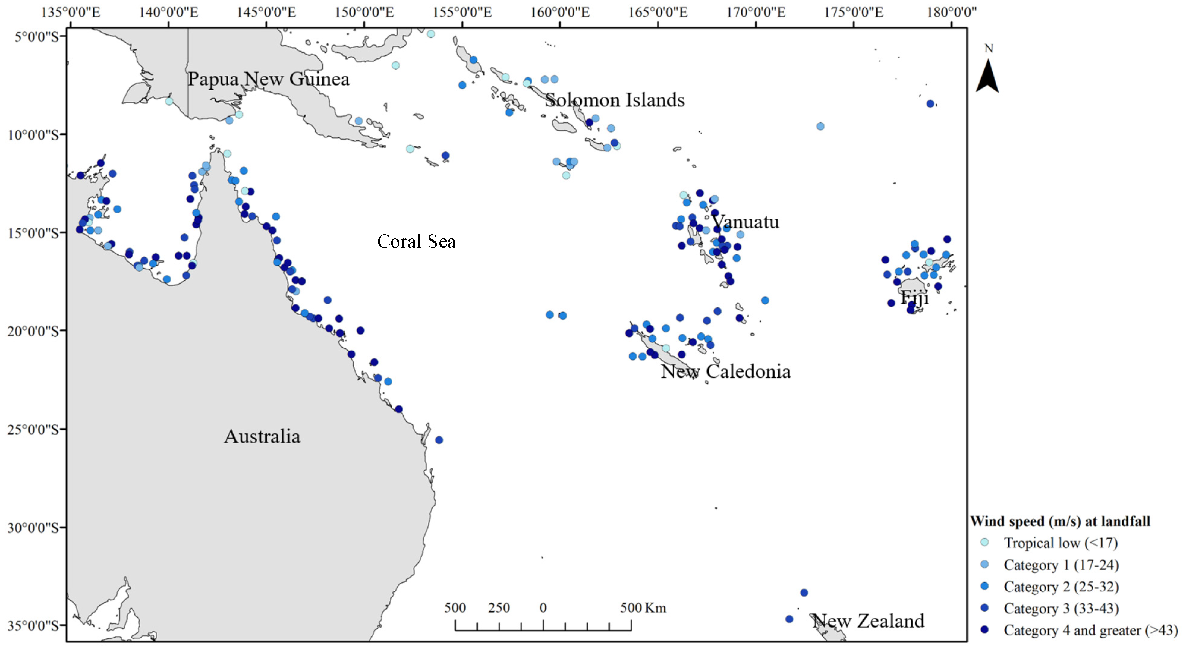
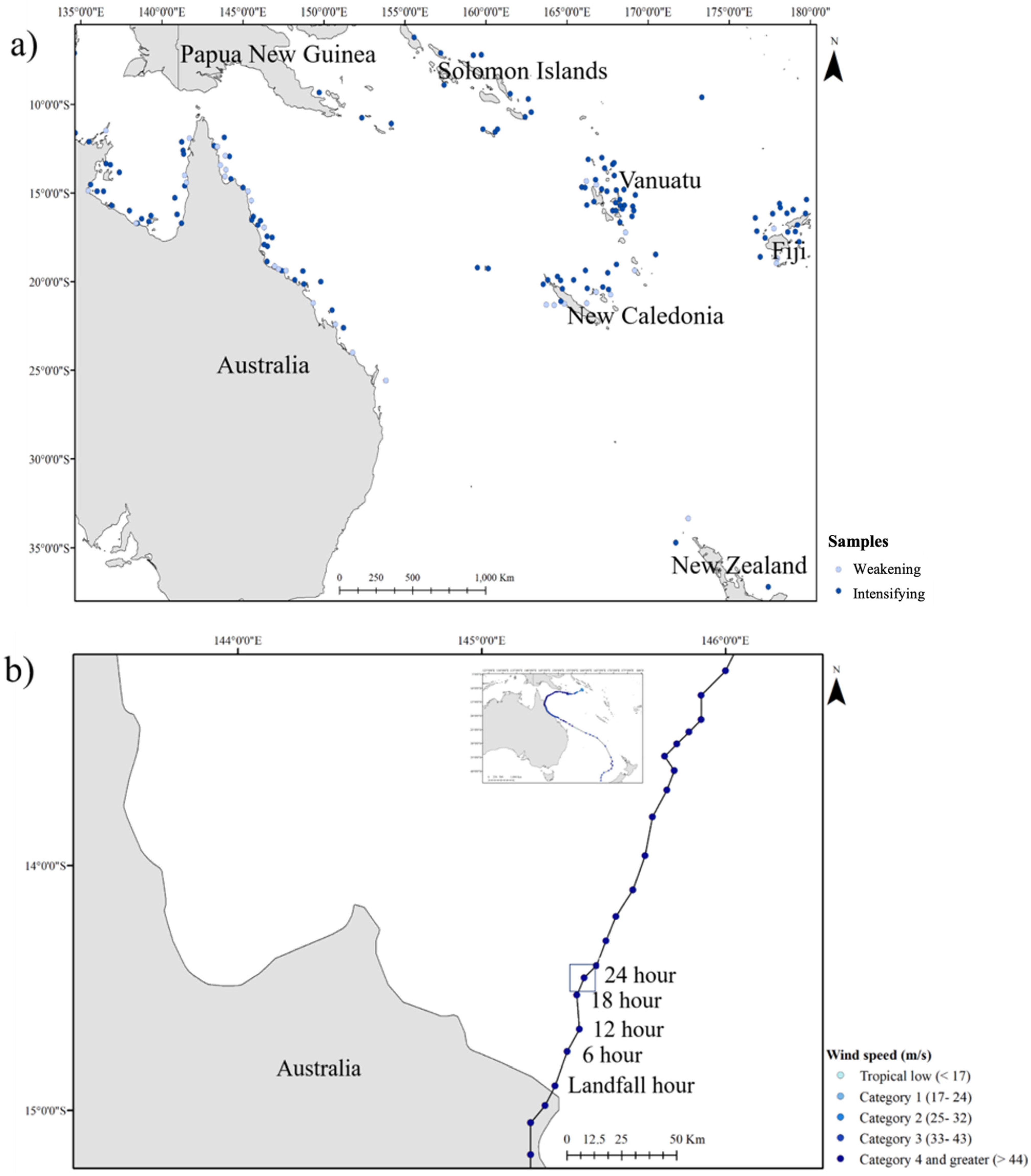
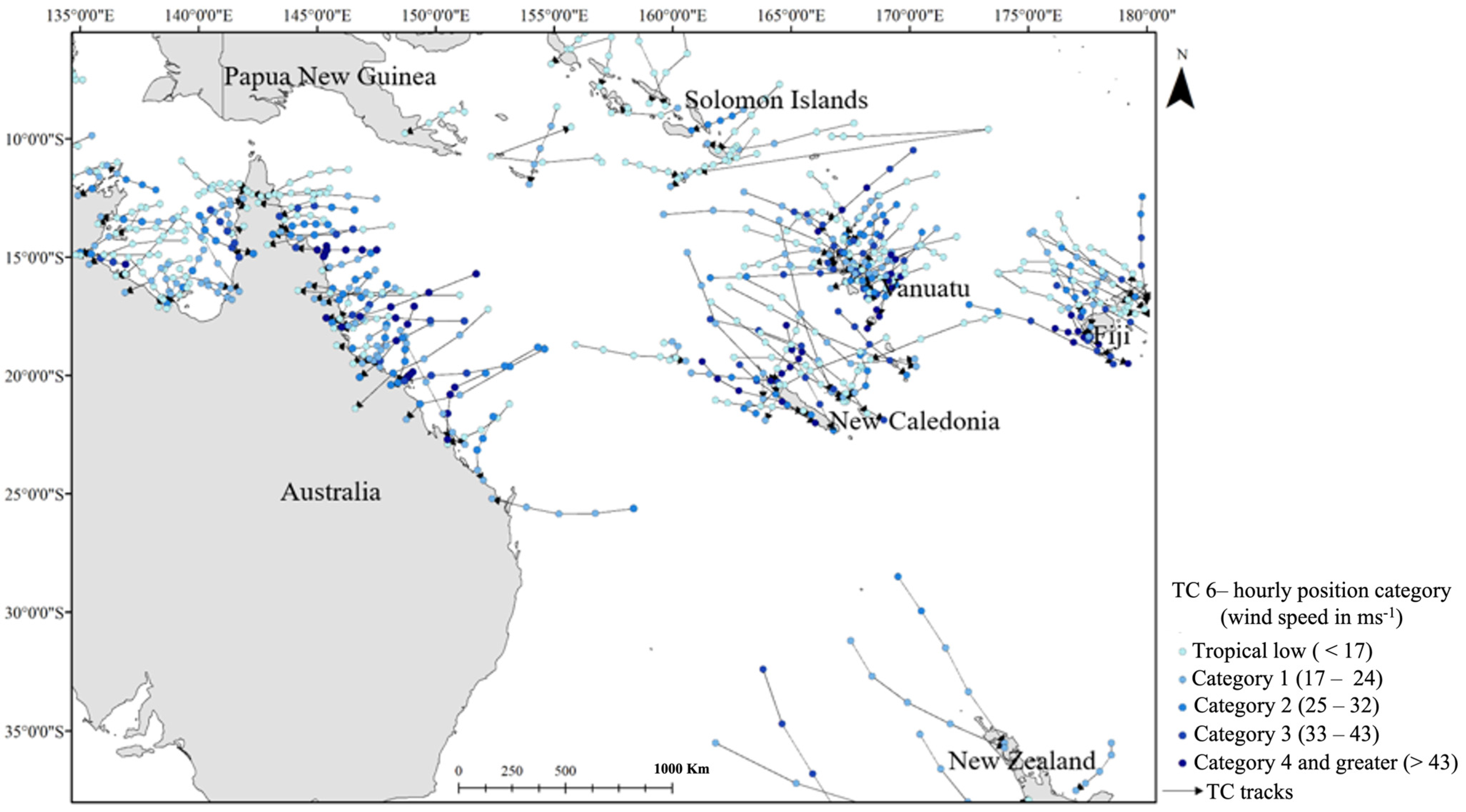
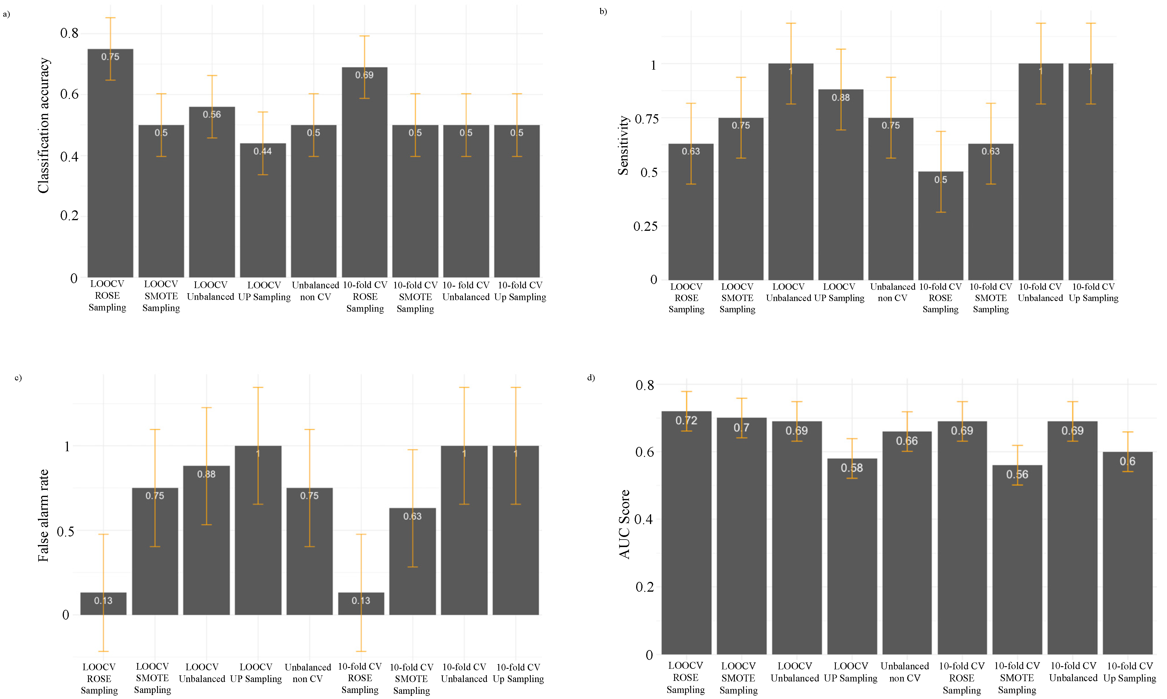
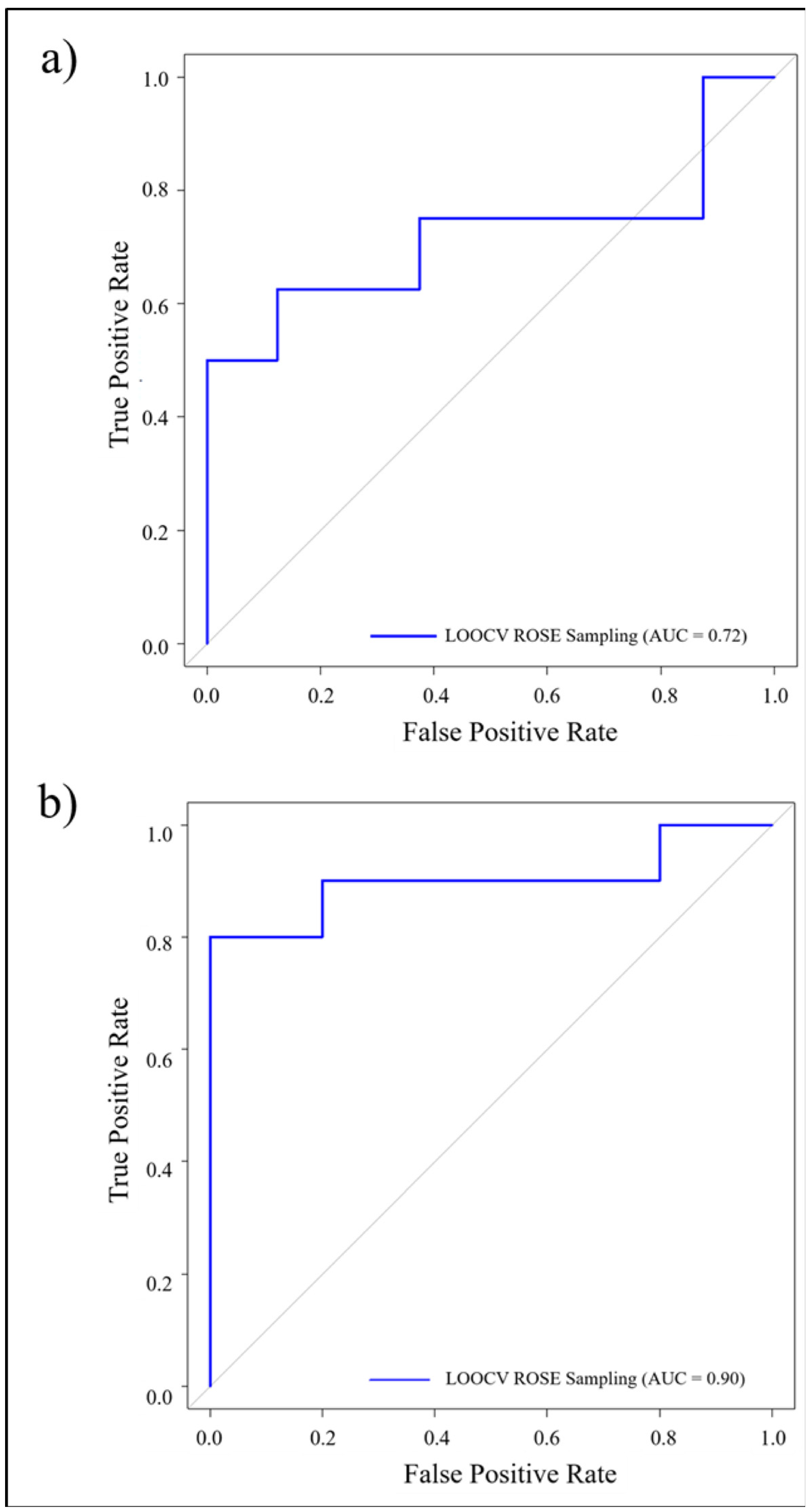
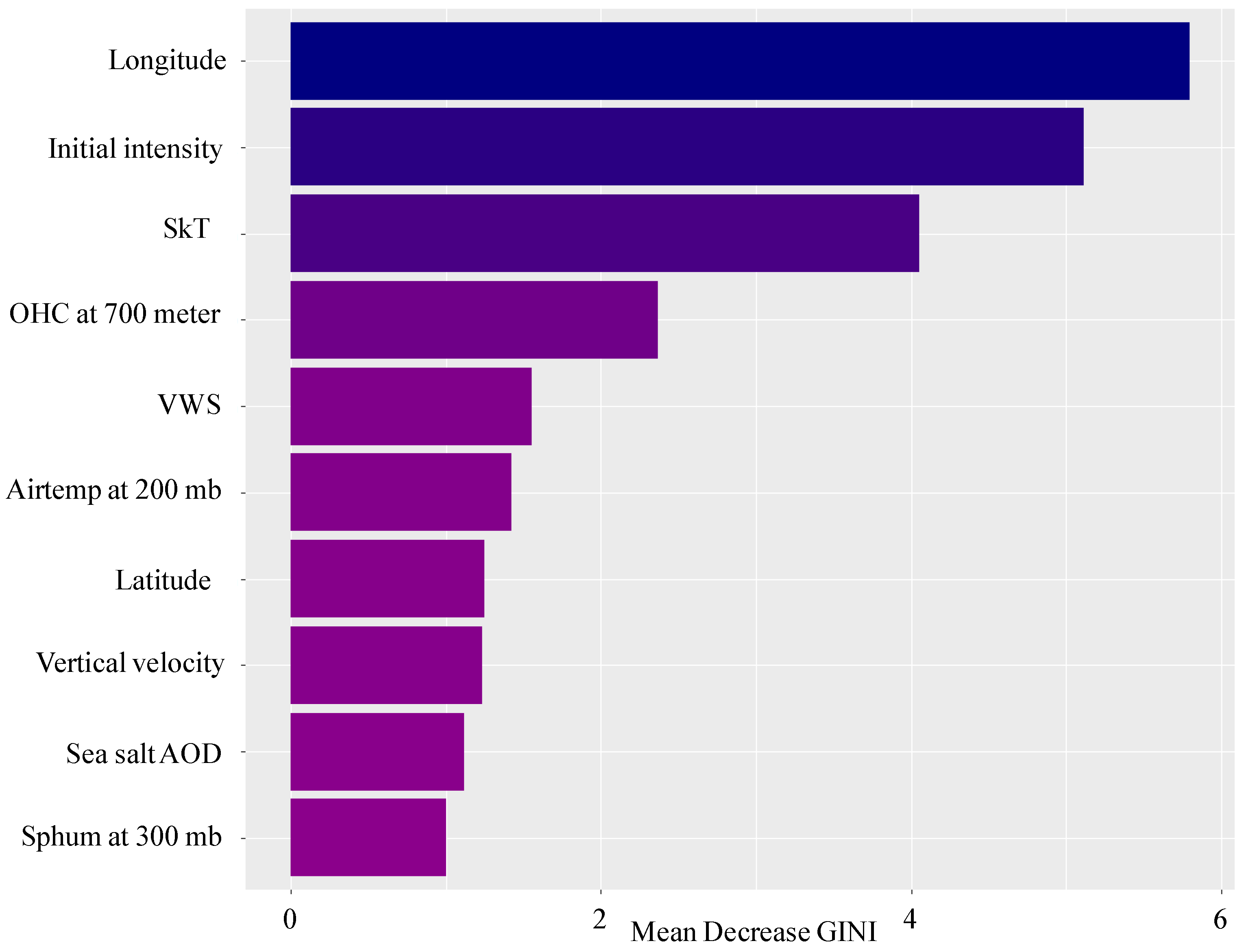
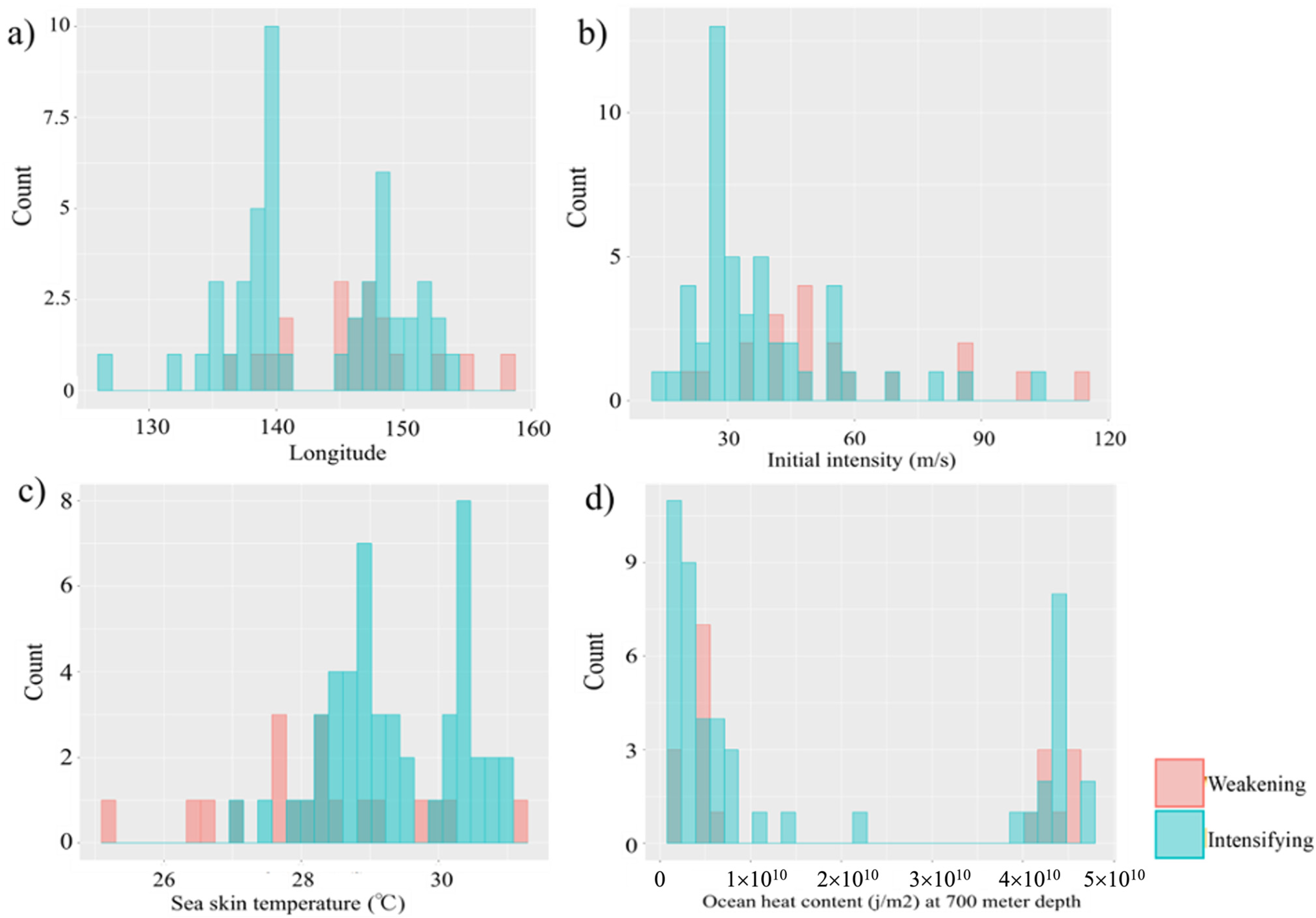
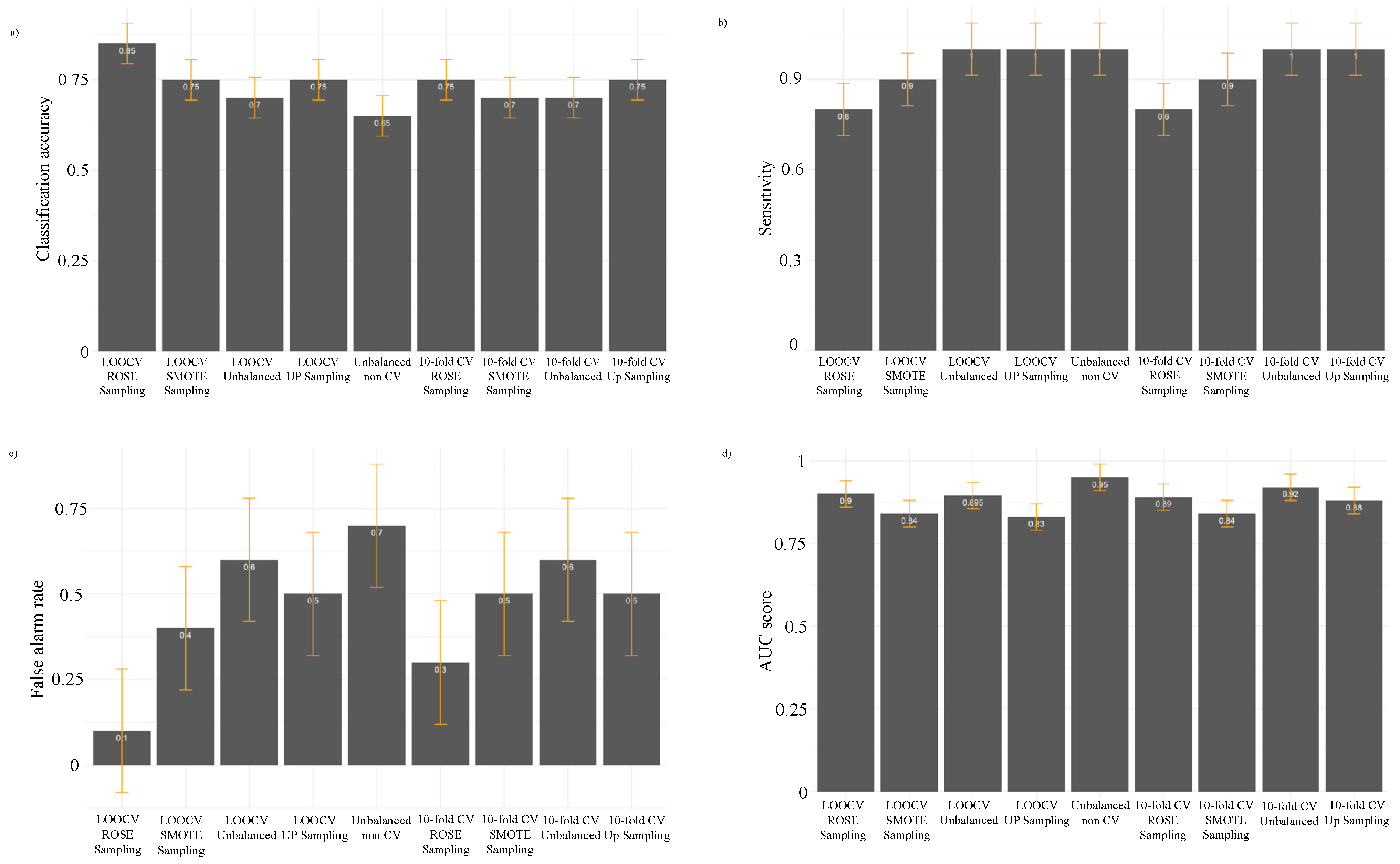
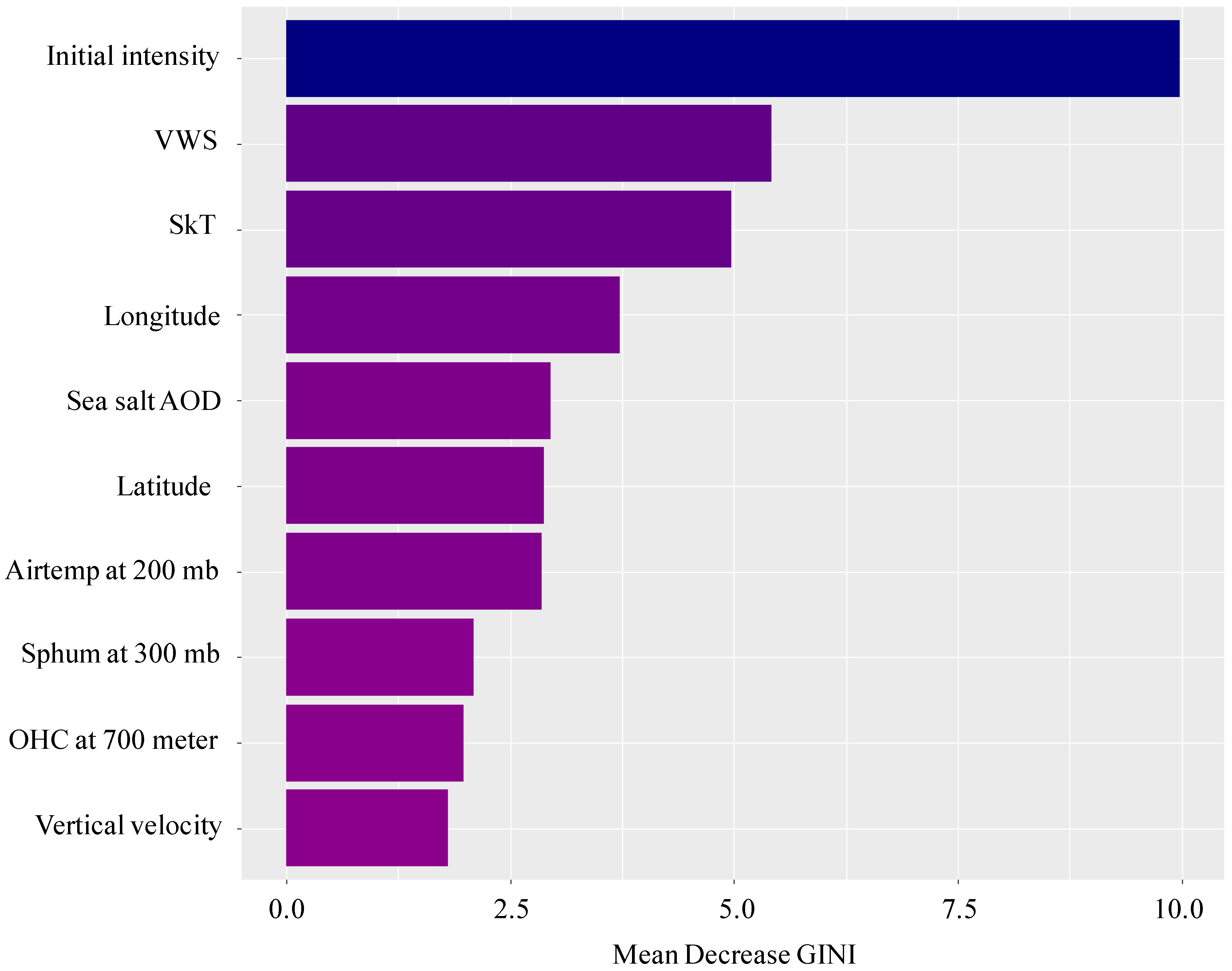
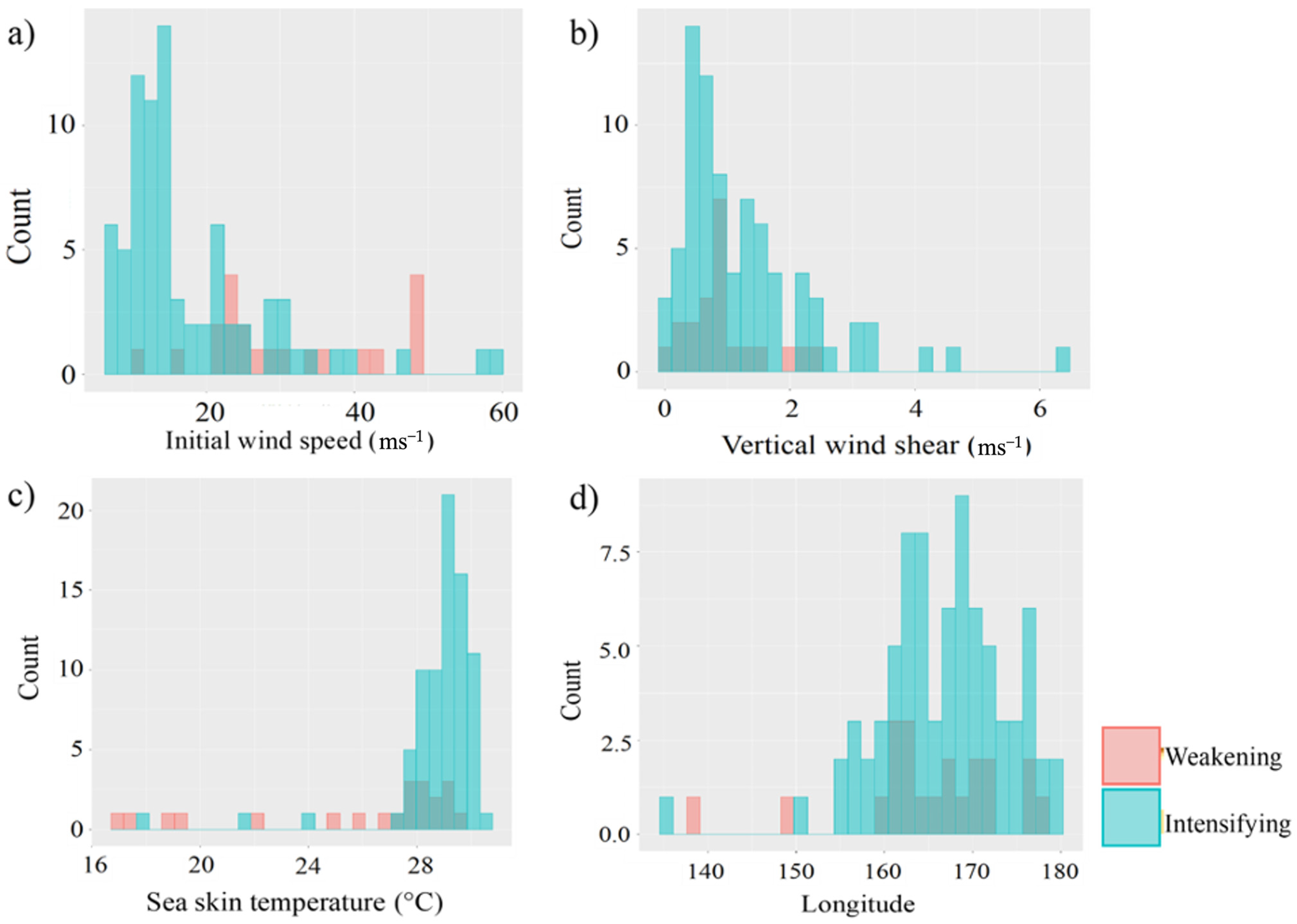
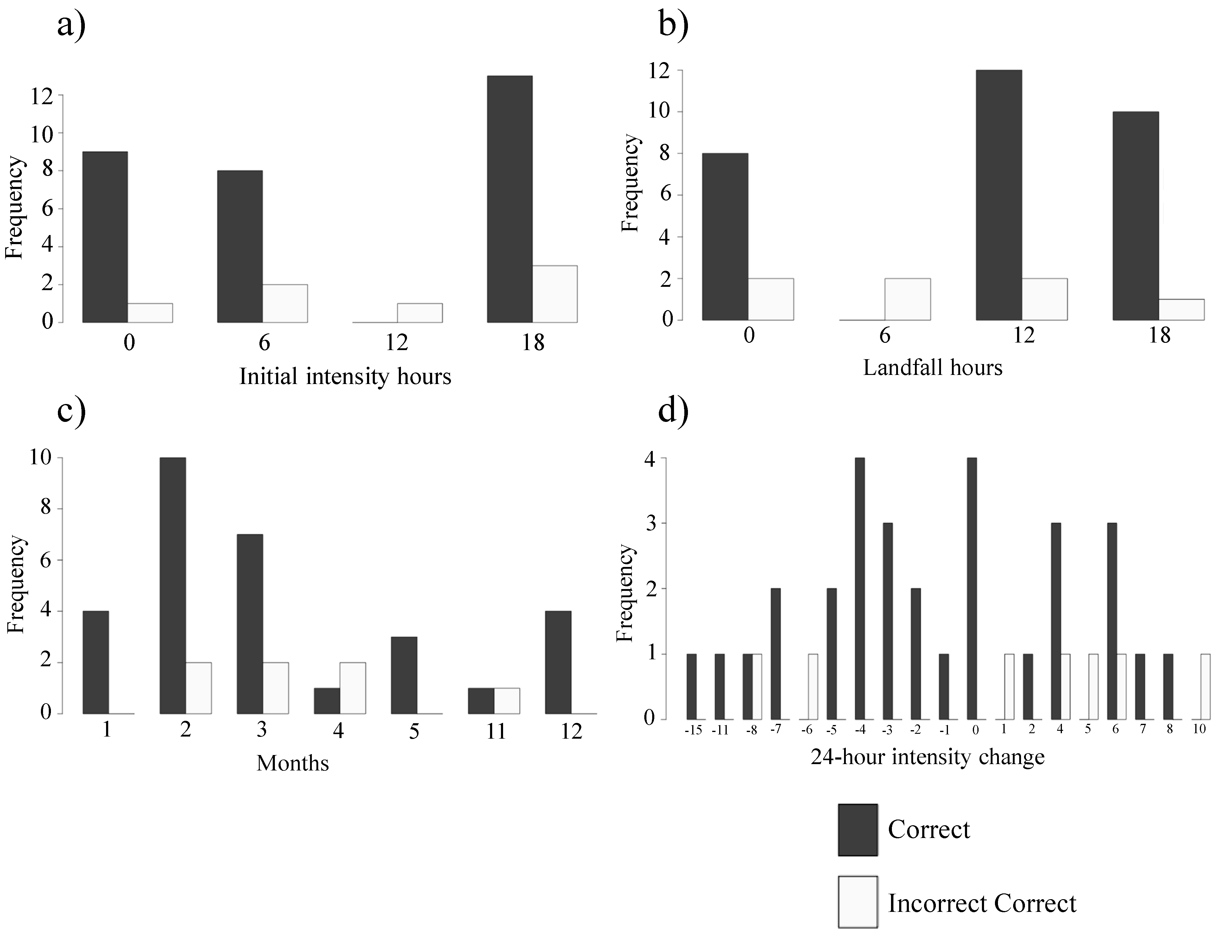
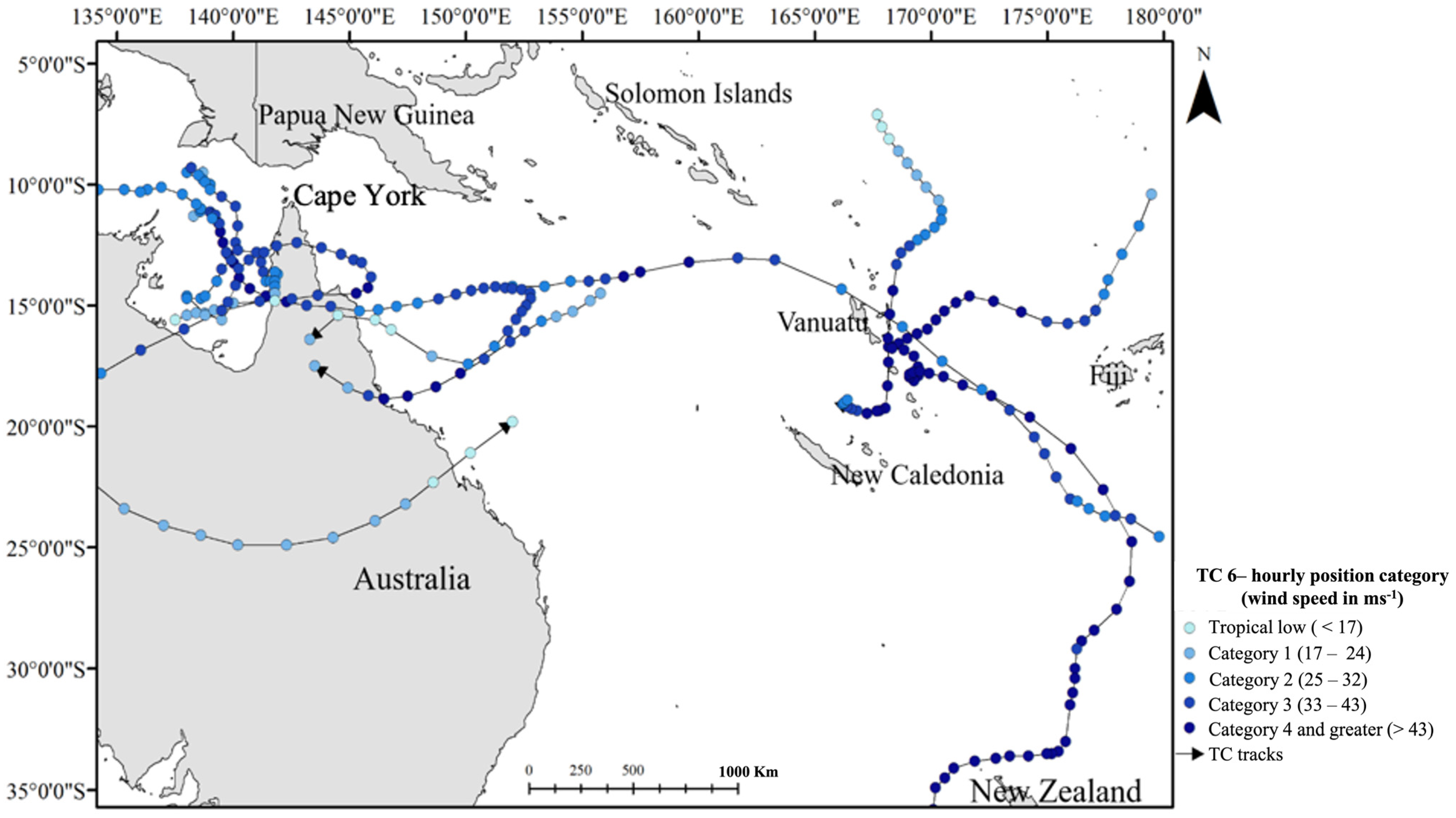
Table 1.
Aerosol and geophysical input variables used in the machine learning algorithms. The table includes the spatial resolution (excluding latitude and longitude) and source of each variable.
Table 1.
Aerosol and geophysical input variables used in the machine learning algorithms. The table includes the spatial resolution (excluding latitude and longitude) and source of each variable.
| Variables | Spatial Resolution | Sources |
|---|---|---|
| Latitude | Point | SPEArTC |
| Longitude | Point | SPEArTC |
| Initial maximum sustained wind speed | Point | SPEArTC |
| Sea surface skin temperature (SkT) | 2.5° × 2.5° | NCEP/NCAR reanalysis |
| Ocean heat content at 700-meter depth (OHC) | 1.0° × 1.0° | ORAS5 |
| Air temperature at 200 hPa (Airtemp) | 2.5° × 2.5° | NCEP/NCAR reanalysis |
| Specific humidity 300 hPa (Sphum) | 2.5° × 2.5° | NCEP/NCAR reanalysis |
| Vertical wind velocity (VW) | 2.5° × 2.5° | NCEP/NCAR reanalysis |
| Vertical wind shear (VWS) | 2.5° × 2.5° | NCEP/NCAR reanalysis |
| Sea salt aerosol extinction optical depth (SSAOD) | 0.5° × 0.625° | MERRA-2 reanalysis |
Table 2.
The confusion matrix reports the number of false positives (FP) model indicates an intensifying storm, when in the real world it was weakening, false negatives (FN)—model indicates a weakening storm, when in the real world it was intensifying, true positives (TP)—model correctly indicates an intensifying storm, and true negatives (TN)—model correctly indicates a weakening storm.
| Actual | |||
| Weakening (0) | Intensifying (1) | ||
| Prediction | Weakening (0) | TN | FN |
| Intensifying (1) | FP | TP | |
Table 3.
Correlation matrix shows p-values between variables at 24 h before SWPO mainland landfall. Significant relationships at 0.05 level are shown in bold.
Table 3.
Correlation matrix shows p-values between variables at 24 h before SWPO mainland landfall. Significant relationships at 0.05 level are shown in bold.
| Latitude | Longitude | Initial Intensity | VW | SSAOD | SH_300 | VWS | SkT | AT_200 | OHC_700 | |
|---|---|---|---|---|---|---|---|---|---|---|
| Latitude | 1 | 1.00 × 10⁻¹³ | 0.1 | 0.61 | 0.26 | 0.46 | 0.1 | 7.00 × 10⁻⁶ | 0 | 0.08 |
| Longitude | 1.00 × 10⁻³ | 1 | 0.01 | 0.85 | 0.19 | 0.55 | 0.57 | 2.00 × 10⁻⁹ | 0.17 | 0 |
| Initial intensity | 1.00 × 10⁻¹ | 0.01 | 1 | 0.79 | 0 | 0.04 | 0.74 | 2.00 × 10⁻³ | 0.23 | 0.02 |
| VW | 6.00 × 10⁻¹ | 0.85 | 0.79 | 1 | 0.56 | 0.39 | 0.58 | 8.00 × 10⁻¹ | 0.71 | 0.81 |
| SSAOD | 3.00 × 10⁻¹ | 0.19 | 0 | 0.56 | 1 | 0.05 | 0.49 | 7.00 × 10⁻¹ | 0.01 | 0.45 |
| SH_300 | 5.00 × 10⁻¹ | 0.55 | 0.04 | 0.39 | 0.05 | 1 | 0.52 | 4.00 × 10⁻¹ | 0 | 0.48 |
| VWS | 1.00 × 10⁻¹ | 0.57 | 0.74 | 0.58 | 0.49 | 0.52 | 1 | 5.00 × 10⁻¹ | 0.56 | 0.16 |
| SkT | 7.00 × 10⁻⁶ | 0 | 0 | 0.78 | 0.7 | 0.38 | 0.5 | 1 | 0.6 | 0 |
| AT_200 | 6.00 × 10⁻⁴ | 0.17 | 0.23 | 0.71 | 0.01 | 0 | 0.56 | 0.6 | 1 | 1 |
| OHC_700 | 8.00 × 10⁻² | 0 | 0.02 | 0.81 | 0.45 | 0.48 | 0.16 | 0 | 1 | 1 |
Table 4.
Correlation matrix shows p-values between variables at 24 h before SWPO island landfall. Significant relationships at 0.05 level are shown in bold.
Table 4.
Correlation matrix shows p-values between variables at 24 h before SWPO island landfall. Significant relationships at 0.05 level are shown in bold.
| Latitude | Longitude | Initial Intensity | VW | SSAOD | SH_300 | VWS | SkT | AT_200 | OHC_700 | |
|---|---|---|---|---|---|---|---|---|---|---|
| Latitude | 1 | 0.04 | 0.02 | 0.78 | 0.00 | 0.08 | 0 | 0.14 | 1 × 10⁻¹⁵ | 0.42 |
| Longitude | 0.04 | 1 | 0.28 | 0.29 | 0.05 | 0.26 | 0.31 | 0.45 | 1 × 10⁻³ | 0.00 |
| Initial intensity | 0.02 | 0.28 | 1 | 0.00 | 0.08 | 0.79 | 0.18 | 0.13 | 7 × 10⁻³ | 0.28 |
| VW | 0.78 | 0.29 | 2 × 10⁻⁷ | 1 | 0.05 | 0.79 | 0.45 | 0.34 | 8 × 10⁻² | 0.27 |
| SSAOD | 0.00 | 0.05 | 8 × 10⁻² | 0.05 | 1 | 0.14 | 0.00 | 0.39 | 1 × 10⁻² | 0.03 |
| SH_300 | 0.08 | 0.26 | 8 × 10⁻¹ | 0.79 | 0.14 | 1 | 0.03 | 0.17 | 5 × 10⁻¹ | 0.32 |
| VWS | 0.00 | 0.31 | 2 × 10⁻¹ | 0.45 | 0.00 | 0.03 | 1 | 0.30 | 0 | 0.34 |
| SkT | 0.14 | 0.45 | 1 × 10⁻¹ | 0.34 | 0.39 | 0.17 | 0.30 | 1 | 0.04 | 0.90 |
| AT_200 | 0.00 | 0.00 | 7 × 10⁻³ | 0.08 | 0.01 | 0.46 | 0.00 | 0.04 | 1 | 0.94 |
| OHC_700 | 0.42 | 0.00 | 3 × 10⁻¹ | 0.27 | 0.03 | 0.32 | 0.34 | 0.90 | 0.94 | 1 |
Table 5.
Confusion matrix for the testing dataset produced from the LOOCV with ROSE sampling random forest with members trained using binary classes for mainland landfall.
Table 5.
Confusion matrix for the testing dataset produced from the LOOCV with ROSE sampling random forest with members trained using binary classes for mainland landfall.
| Reference | |||
| Weakening | Intensifying | ||
| Prediction | Weakening | 7 | 3 |
| Intensifying | 1 | 5 | |
Table 6.
Confusion matrix for the testing dataset produced from the LOOCV with ROSE sampling random forest with members trained using binary classes for island landfall.
Table 6.
Confusion matrix for the testing dataset produced from the LOOCV with ROSE sampling random forest with members trained using binary classes for island landfall.
| Reference | |||
| Prediction | Weakening | Intensifying | |
| Weakening | 9 | 2 | |
| Intensifying | 1 | 8 | |
Table 7.
Number of incorrect predictions from island and mainland models, their landfall date and time, geographic location, Vmax, actual class and predicted class.
Table 7.
Number of incorrect predictions from island and mainland models, their landfall date and time, geographic location, Vmax, actual class and predicted class.
| Landfall Location | Name | Landfall Date and Time | Latitude | Longitude | Vmax (ms−1) | Actual Class | Predicted Class |
|---|---|---|---|---|---|---|---|
| Island | VELI | 8 February 1987 0:00 | −14.33 | 166.17 | 15 | 0 | 1 |
| BOLA | 28 February 1988 12:00 | −16.64 | 168.25 | 38 | 1 | 0 | |
| VANIA | 15 November 1994 0:00 | −15.36 | 168.24 | 25 | 1 | 0 | |
| Mainland | GILLIAN | 10 March 2014 6:00 | −14 | 141.4 | 15 | 0 | 1 |
| DOMINIC | 7 April 1982 6:00 | −14.6 | 141.4 | 34 | 1 | 0 | |
| ETHEL | 9 March 1996 12:00 | −12.8 | 141.33 | 21 | 1 | 0 | |
| TESSI | 2 April 2000 18:00 | −18.86 | 146.48 | 29 | 1 | 0 |
Disclaimer/Publisher’s Note: The statements, opinions and data contained in all publications are solely those of the individual author(s) and contributor(s) and not of MDPI and/or the editor(s). MDPI and/or the editor(s) disclaim responsibility for any injury to people or property resulting from any ideas, methods, instructions or products referred to in the content. |
© 2023 by the authors. Licensee MDPI, Basel, Switzerland. This article is an open access article distributed under the terms and conditions of the Creative Commons Attribution (CC BY) license (https://creativecommons.org/licenses/by/4.0/).
Share and Cite
MDPI and ACS Style
Bhowmick, R.; Trepanier, J.C.; Haberlie, A.M. Classification Analysis of Southwest Pacific Tropical Cyclone Intensity Changes Prior to Landfall. Atmosphere 2023, 14, 253. https://doi.org/10.3390/atmos14020253
AMA Style
Bhowmick R, Trepanier JC, Haberlie AM. Classification Analysis of Southwest Pacific Tropical Cyclone Intensity Changes Prior to Landfall. Atmosphere. 2023; 14(2):253. https://doi.org/10.3390/atmos14020253
Chicago/Turabian StyleBhowmick, Rupsa, Jill C. Trepanier, and Alex M. Haberlie. 2023. "Classification Analysis of Southwest Pacific Tropical Cyclone Intensity Changes Prior to Landfall" Atmosphere 14, no. 2: 253. https://doi.org/10.3390/atmos14020253
Note that from the first issue of 2016, this journal uses article numbers instead of page numbers. See further details here.