
Sensitivity of Ozone Formation in Summer in Jinan Using Observation-Based Model

1
Department of Earth System Science, Ministry of Education Key Laboratory for Earth System Modeling, Institute for Global Change Studies, Tsinghua University, Beijing 100084, China
2
Institute of Atmospheric Physics, Chinese Academy of Sciences, Beijing 100029, China
3
Jinan Ecological Environment Monitoring Center of Shandong Province, Jinan 250000, China
4
Jinan Bureau of Ecology and Environment, Jinan 250098, China
*
Author to whom correspondence should be addressed.
Atmosphere 2022, 13(12), 2024; https://doi.org/10.3390/atmos13122024
Submission received: 20 October 2022
/
Revised: 24 November 2022
/
Accepted: 27 November 2022
/
Published: 1 December 2022
(This article belongs to the Section Air Pollution Control)
Abstract
:According to online monitoring data on atmospheric ozone and the pollution characteristics of its precursors obtained in Jinan in June 2021, we analyzed different sites: urban sites (city monitoring station, Quancheng Square), an industrial park site (oil refinery), and a suburban site (Paomaling). The relative incremental reactivity of different precursors was calculated using a photochemical observation-based model to explore the sensitivity of O3 generation at each site and to draw a curve using the empirical kinetics modeling approach. The PMF model was used to analyze the origin of volatile organic compounds (VOCs) pollution in Jinan. The results showed that the concentration of O3 at the industrial park was higher than that in the urban area in Jinan, which may be related to the fact that ozone precursor concentrations in the industrial park were significantly higher than those in the urban area (the AVOCs concentration at the industrial park site was 56.9 ppbv, approximately twice that of the urban site), and there are emission peaks at night; alkanes, oxygenated compounds, and halogenated hydrocarbons were the main components of the AVOCs, and olefins, alkanes, and aromatic hydrocarbons were the main active components in Jinan. The O3 generation in urban areas generally occurred in the VOCs-sensitive zones, while the O3 generation in the other areas occurred in the VOCs-NOx transition zone; there was a clear diurnal variation in the sensitivity of the industrial park, with the site being in the obvious VOCs-sensitive zone from nighttime to morning hours and shifting to the VOCs-NOx transition zone in the afternoon hours; the relative incremental reactivity (RIR) value of AVOCs for O3 generation in Jinan was the largest, and olefins were the most sensitive component of O3. The AVOCs in Jinan mainly originated from motor vehicle exhaust, oil and gas volatilization, industrial emissions, and solvent use, and ozone prevention and control in summer should strengthen the control of these sources.
1. Introduction
Tropospheric ozone (O3), being a key component of atmospheric photochemical smog, is a secondary pollutant generated from photochemical reactions by a precursor of volatile organic compounds (VOCs), NOx, and CO in the atmosphere [1,2]. Many studies have shown that high concentrations of O3 near the ground are harmful to human health and the growth of animals and plants [3]. They also negatively impact the climate and the ecological balance [4]. A study of 95 cities in the United States showed that the risk of death in a given population may increase by 0.52% (95% CI: 0.27–0.77%) for every 5.1 μg/m3 increase in the daily O3 concentration [5]. High concentrations of O3 induce damage to plant leaves, accelerate plant senescence, reduce photosynthesis capacity, and reduce ecosystem carbon sink capacity, thereby affecting the ecological balance [6,7].
In recent years, the concentrations of O3 in the key cities of China have shown an upward trend, and O3 has gradually become the primary air pollutant [8]. There is a strong nonlinear relationship between the O3 concentration and the emission of specific atmospheric precursors (e.g., VOCs and NOx). It is thus important to study the relationship between O3 and its precursors for the formulation of O3 pollution prevention and control strategies [9]. Primary pollution would be reduced by precursors control measures, but O3 concentrations may be still increased. Studies have shown that summertime O3 concentrations increased by approximately 2 ppbv/yr from 2003 to 2015 in North China, although urban NOx emissions have greatly reduced since 2012.
Scientific research on the reaction mechanism and pollution prevention of O3 and its precursors has been carried out in many cities in China, including on the photochemical reaction mechanism of O3 [10,11], the sensitivity of O3 and its precursors (VOCs, NOx) [12,13], the contribution of local and regional transport [14], the emission of O3 precursors, the correlation between O3 pollution and meteorology [15], and the effect of O3 on human health [16]. Most studies have shown that the formation of O3 is controlled by VOCs in large Chinese cities, such as Beijing [1], Shanghai [17], Shenzhen [18], Nanjing [19], and Chengdu [2]. Furthermore, VOCs with high O3 formation potential are largely alkenes and aromatic hydrocarbons. On the contrary, the formation of O3 is controlled by NOx in some suburbs or rural areas, such as Taishan, the suburbs of Guiyang, and Yanshan, which have higher VOC emissions from natural sources [20,21,22]. Some studies have reported temporal and spatial differences in the sensitivity of O3 and its precursors, which could vary across place and time. For example, studies in Beijing–Tianjin–Hebei, the Yangtze River Delta, and the Pearl River Delta have found that the local formation of O3 is VOC-sensitive in the morning and NOx-sensitive in the afternoon [22,23,24]. In addition, there may be differences across cities, suburbs, and outer suburbs at the same time. Generally, cities are VOC-sensitive, the outer suburbs are NOx-sensitive, and the inner suburbs are VOCs-NOx-sensitive [25,26].
Jinan is located in the central and western parts of Shandong Province. The urban area is surrounded by Mount Tai in the south and presents an elevated landform in the south and north. The frequency of the temperature inversion is high, and the wind speed is low, which makes the region prone to the accumulation of pollutants. The air pollution in the city and surrounding areas is relatively serious [27]. During the 13th 5-Year Plan, the air quality in Jinan improved significantly, the annual average concentration of PM2.5 decreased by 42.7%, and the number of days with good air quality increased by 13.8%. However, the annual 90th percentile of the highest 8 h daily concentration of O3 increased by 5.1%. In 2020, the annual average concentration of O3 was 185 μg/m3, ranking 8th from the bottom among the 337 cities in the country. As an important city in the air pollution transmission channel of Beijing–Tianjin–Hebei, Jinan has sufficient data on meteorological parameters and air pollutant monitoring, but research on O3 pollution is obviously less than in other key cities, such as Beijing, Shanghai, and Shenzhen. In this study, the pollution characteristics of O3 and its precursors were analyzed at four different field sites in Jinan in June 2021. An observation-based model (OBM) was used to identify the sensitivity and control factors. Positive matrix factorization (PMF) was used to analyze the sources of VOCs. The findings of this study are expected to provide a scientific basis for the refinement of local pollution prevention and control policies for O3 and its precursors.
2. Methods and Data
2.1. Field Measurements
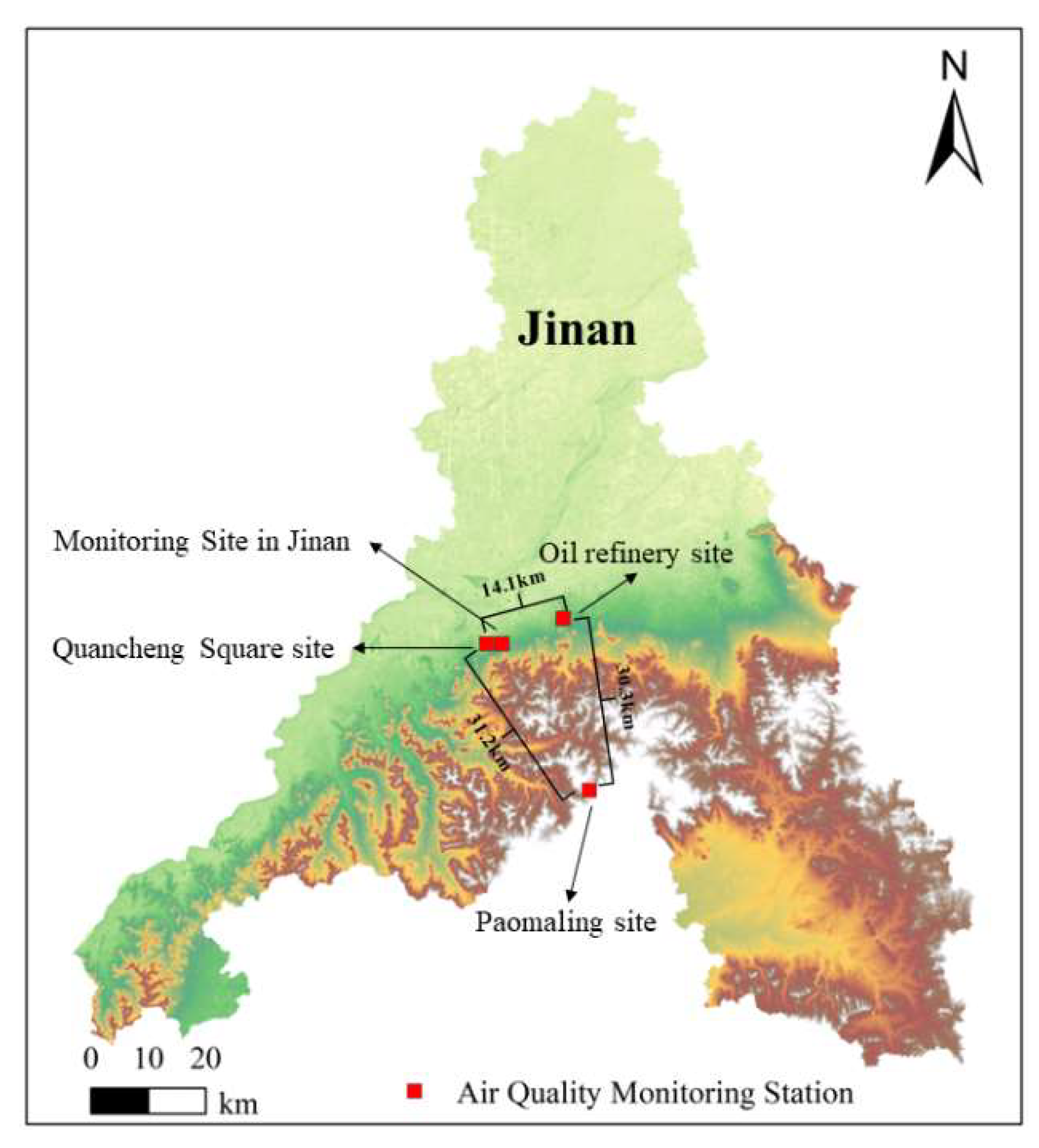
This study presents the results from a field campaign conducted in Jinan in June 2021. Four stations were set-up in different pollution source areas: a monitoring site in Jinan (117.05° E, 36.66° N); Quancheng Square site (117.02° E, 36.66° N), an oil refinery site (117.17° E, 36.70° N), and Paomaling site (117.22° E, 36.43° N). As shown in Figure 1, the city monitoring station (MS) and Quancheng Square (QCS) were located in an urban area of Jinan city, where their surroundings comprised traffic sources; therefore, they were the representative stations of the urban area. The refinery site was located around a refinery in an industrial park, serving as the representative site of the industrial area. There was no obvious anthropogenic source around the Paomaling site (PML), mainly due to the presence of vegetative influences and, thus, it was representative of the suburbs.
The VOC species were detected and analyzed by GC-MS/FID, including 107 components of PAMS and TO-15. The MS and QCS adopted the Shanghai Panhe automatic monitor for VOCs; OL and PML adopted the Wuhan Tianhong automatic monitor for VOCs. For each sample analysis, four internal standard compounds (i.e., bromochloromethane, 1,4-difluorobenzene, deuterated chlorobenzene, and 4-bromofluorobenzene) were used for an internal standard method of quantification. The quantitative calibration curve gradient was 0.5, 1.0, 2.0, 5, 15, and 20 ppbv linear regression acquisition. The middle point of the curve was calibrated once every morning to ensure that the deviation was not greater than 30%, otherwise, the standard curve was redrawn for calibration. The conventional pollutants (i.e., SO2, NO2, CO, O3, PM2.5, and PM10) and meteorological parameters (i.e., wind direction, wind speed, temperature, humidity, and atmospheric pressure) were obtained from the site’s automatic monitoring network data. The monitoring equipment was automatically calibrated every morning. All monitoring data were updated every hour.
2.2. Ozone Formation Potential (OFP)
In the atmosphere, the amount of O3 generated from reactions depends on many factors, such as the concentration of VOCs and NOx, the atmospheric oxidation rate, and the specific oxidation mechanism. Carter proposed the concept of VOCs’ incremental reaction (IR, g O3/g VOCs) to evaluate the contribution of various VOCs to O3 generation, which was used to measure the change in O3 by changing the amount of VOCs [28]. The maximum incremental reactivity (MIR) was obtained by changing the VOCs/NOx ratio. The MIR is generally used to calculate the OFP values of the different VOC species to estimate their activity and ability for O3 generation [29]. The OFP was calculated using the following formula [8].
In the formula, represents the OFP value corresponding to species i of the VOCs; represents the concentration of species i of the VOCs in ppbv; represents the MIR value of species i of the VOCs, and it is dimensionless. The MIR data were obtained from reference [30].
2.3. Observation-Based Model (OBM)
The OBM model was based on observational data to simulate atmospheric photochemical reactions, where the input of the data comprised hourly concentrations of NO, NO2, CO, SO2, and VOCs species. The hourly values of meteorological parameters, such as relative humidity, air pressure, and temperature, were also used with the CB05 mechanism to simulate and obtain the output. The VOC species included alkanes, alkenes, aromatic hydrocarbons, and oxygen compounds. Data on the photochemical reaction-related parameters were used by the model to simulate the chemical process of the atmospheric reactions and to inversely deduce the relationship of the precursor VOCs, NOx, and O3 [29]. Usually, the empirical kinetics modeling approach (EKMA) curve is used to identify the sensitive area of O3 generation, and the relative incremental reactivity (RIR) is used to identify the sensitivity of the different kinds of precursors to O3 generation.
2.3.1. Empirical Kinetics Modeling Approach (EKMA)
The EKMA curve is an expression of ozone generation concentration simulated by a photochemical reaction model. It is an isoconcentration curve graph drawn based on the concentration data of ozone, VOCs, and NOx, which can be used to express the relationship between ozone and the concentrations of its two precursors, NOx and VOCs [29]. The inflection point connection of the contour lines is the ridge line of the EKMA curve. Normally, NOx is taken as the ordinate and VOCs as the abscissa. When it is above the ridge line, O3 is generated in the VOC-sensitive area; controlling the VOCs emission is beneficial for reducing the O3 generation. When it is below the ridgeline, the O3 generation is in the NOx-sensitive area, and controlling the NOx emissions is conducive to reducing the O3 generation [31].
2.3.2. Relative Incremental Reactivity (RIR)
The RIR was used to explore the sensitivity relationship between O3 and different precursors, and it is expressed as the ratio between the rate of change (%) of the photochemical generation rate of O3 and the rate of change (%) of the source. When the RIR is positive, this indicates that controlling such a precursor can effectively reduce the generation of O3. The larger the value, the more sensitive the precursor is to the generation of O3 [32]. The RIR can be calculated as follows:
where is the relative incremental reactivity of precursor ; is the generation rate of the daytime (07:00~19:00) O3; denotes the NO, CO, AVOCs (artificial source VOCs), and any other O3 precursors; is the change in the concentration of species . is the O3 formation rate corresponding to the change in the concentration of the species . In the simulation process of this study, was selected as 10% of , and the net production rate of O3 () was calculated by using the OBM simulation output parameters [33].
The production of O3 mainly depends on the degree of the photochemical reaction [32]. The net production rate of O3 () can be calculated by the difference between the gross production ( and the destruction (. is calculated by the oxidation of NO by HO2 and RO2. Peroxyradicals (HO2, RO2) oxidize NO to produce NO2, and then photolysis occurs to produce O3. Concurrently, O3 can be destructed through photolysis and in the reaction with alkenes, HO2, and OH [32]. All radicals and intermediates were obtained from the outputs of the OBM. The constants (k) represent the rate of each reaction.
2.4. Positive Matrix Factorization (PMF) Model
In this study, the PMF5.0 model recommended by USEPA was used for the source analysis of atmospheric VOCs. When running the model, the hourly concentration of VOC species with pollution source characteristics was used as the input. Most of the residuals of the VOC species in the analysis results were between −3.0 and 3.0. When the signal-to-noise ratio of the VOCs species was greater than 1, it was defined as strong (Strong) and could be directly fed into the model calculation. When it was between 0.5 and 1, it was defined as weak (Weak), and the species uncertainty set in the input model file was multiplied 3 times. When the signal-to-noise ratio of the VOCs species was less than 0.5, it was defined as bad (Bad) and was not included in the model calculation [34].
The VOC components involved in the model calculation had high signal-to-noise ratios (greater than 2) and fewer missing values to reduce the impact of data measurement errors on the PMF analysis. The selected species were required to have a high-volume fraction and a strong source indication to reduce the uncertainty caused by the initial volume fraction calculation. The species with very high reactivity were not selected.
3. Results and Discussion
3.1. VOC Pollution Characteristics
3.1.1. Meteorological Condition and Pollution Characteristics
In June 2021, Jinan city has accumulated 14 days of mild O3 pollution (100 ppbv ≥ O3 maximum 8-h average > 75 ppbv), and eight days of moderate pollution (124 ppbv ≥ O3 maximum 8-h average > 100 ppbv). In terms of hourly concentration, there was a total of 93 h of O3 mild pollution (140 ppbv ≥ O3 hourly concentration > 93 ppbv) in June 2021, and the monthly average O3 maximum 8-h 90th percentile concentration was 106.4 ppbv. The average temperature in Jinan was 27.1 °C, and the relative humidity was 55.9%. A high temperature and low humidity are favorable for ozone formation. The meteorological parameters and pollutant concentrations of the four component monitoring stations are shown in Table 1. From the perspective of meteorological conditions, the stations in the urban area (i.e., city monitoring station (MS) and Quancheng Square (QCS)) and the industrial park (refinery (or)) were cleaner than the stations (Paomaling (PML)) with a higher temperature and lower humidity. The meteorological conditions were more conducive to O3 generation. In terms of the pollutant concentration, the industrial park site (Refinery) had the highest O3 concentration, and the monthly average (90th percentile of the highest 8-h daily) concentration of O3 was 118.1 ppbv, followed by the urban site (i.e., city monitoring station and Quancheng Square), with a concentration of approximately 114 ppbv. The clean site (i.e., Paomaling) had the lowest O3 concentration (92.3 ppbv). For NOx, the urban stations were affected by motor vehicle emissions, and the concentration was slightly higher than that of the industrial park stations. The NOx concentration in Quancheng Square was the highest (17.1 ppbv), and that at the clean stations was the lowest (4.6 ppbv). For AVOCs, affected by surrounding industries and certain combustion emissions, the concentration of AVOCs in the industrial park station was 56.9 ppbv, which was approximately twice that of the urban station. In addition, the average concentration of isoprene at each station was low, which shows that the ozone pollution in Jinan in summer was not significantly affected by natural sources.
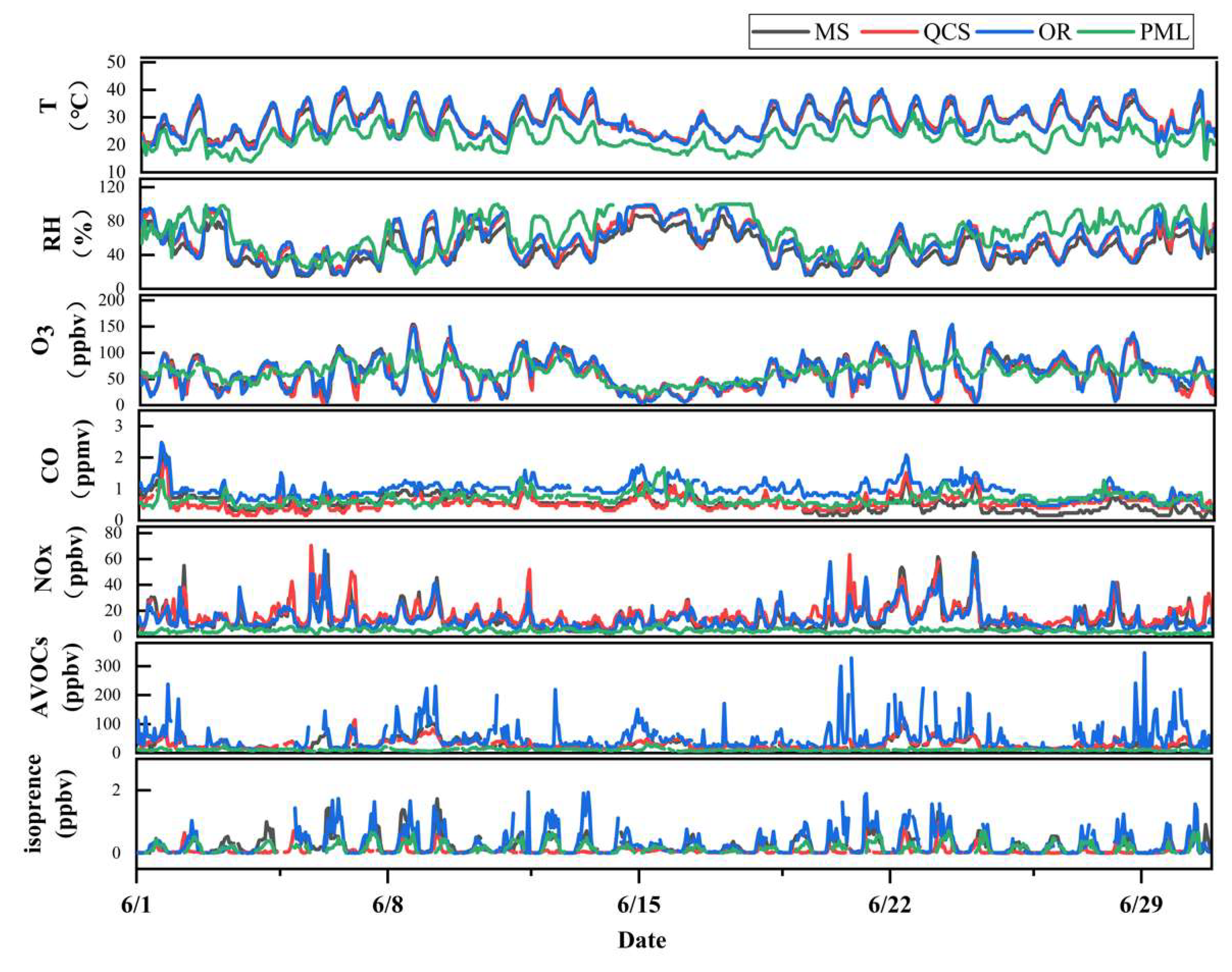
Figure 2 shows the daily changes in the meteorological parameters and pollutant volume fractions at each station in Jinan over the observation period. In the summer of 2021, the precursor NOx and VOCs in Jinan at night and in the morning had high concentrations. When the hourly temperature in the afternoon reached above 35 °C, the hourly concentration of O3 easily exceeded the standard. As shown in Figure 1, the AVOCs concentration at the industrial park site in Jinan city exceeded 200 ppbv at 20:00–22:00 and 02:00–05:00 on 20–24 June. Meanwhile, the maximum hourly NOx concentration in the morning from 06:00 to 08:00 exceeded 40 ppbv, and the daily maximum temperature reached 38~40 °C. In the afternoon, the maximum hourly O3 concentration reached approximately 120 ppbv~140 ppbv. However, Jinan city was in O3 pollution day from 20 to 24 June and reached O3 moderate pollution.
In addition, the analysis of the pollutant concentration at each station shows that there were obvious high concentrations of AVOCs and NOx at night at all stations in Jinan Industrial Park, which may have been the result of industrial enterprises secretly discharging at night. In order to control the ozone concentration at this station under high-temperature conditions, the supervision of industrial enterprises at night should be strengthened.
3.1.2. Diurnal Variation
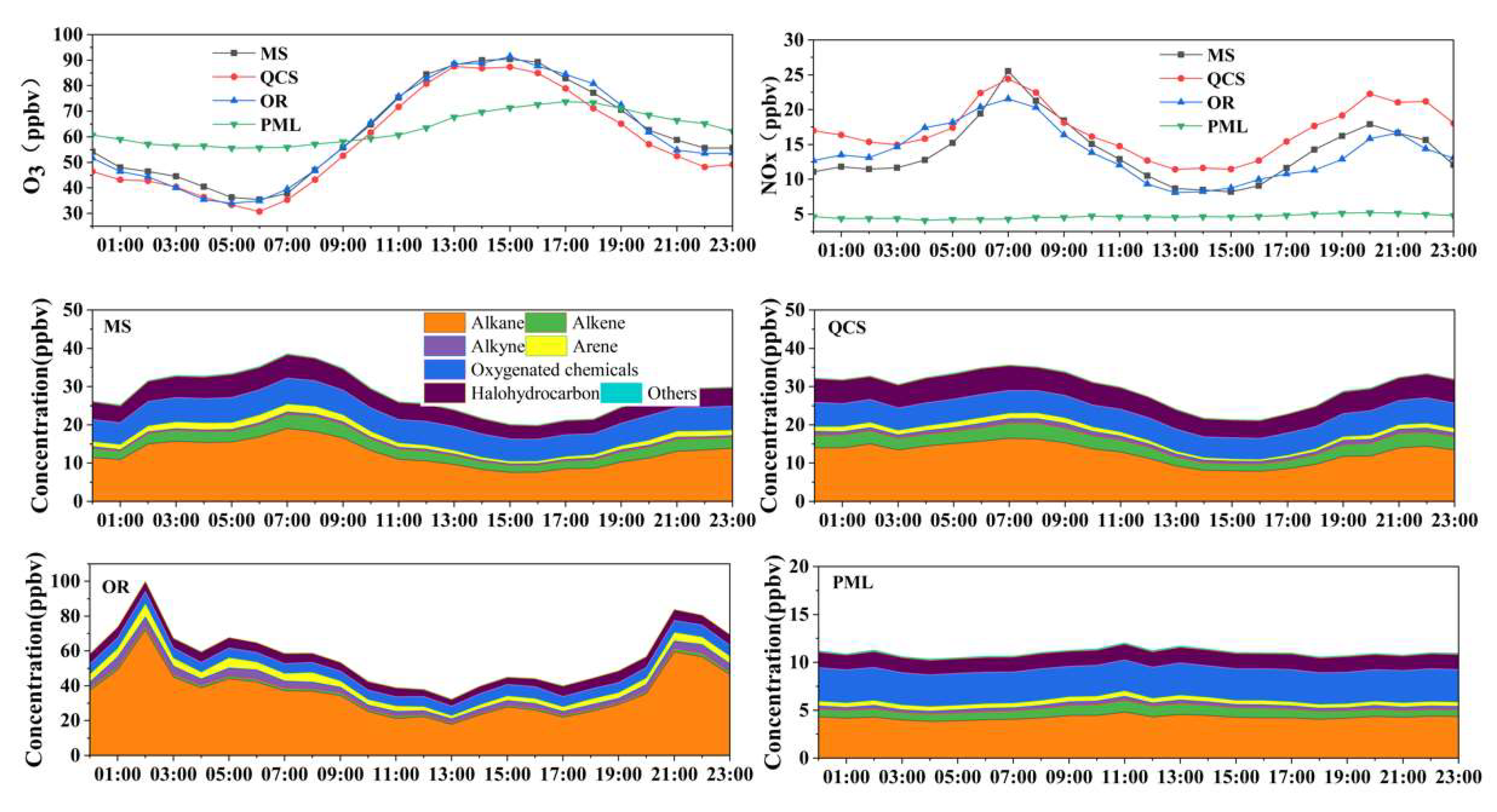
O3 and its main precursors are affected by several factors, such as the source of emissions, photochemical reactions, and atmospheric boundary layer movement, which show significant daily variation [35]. The average daily variation in pollutant concentrations at each site in Jinan city is shown in Figure 3. The daily concentrations of O3 in urban areas and industrial parks showed a unimodal change. The concentrations began to increase at 06:00, reached a peak at 15:00, and then gradually decreased. Among these, the hourly peak concentration of O3 at the industrial park was higher than that in the urban areas. The diurnal variation of O3 in the suburbs was relatively gentle due to the significantly lower emissions of precursors than at the other sites. The peak concentration was significantly lower than that in the urban areas and industrial parks as well. However, from night to early morning, when sun exposure was weak, the emissions of NO in the urban areas and industrial parks were higher than those in the suburban areas. NO reactions that consume O3 occurred at night which, in turn, leads to lower O3 concentrations in urban areas and industrial parks than in suburban areas.
The daily concentration of NOx in the urban areas and industrial parks showed an obvious bimodal change, where a peak occurred between 07:00 and 20:00. There was an obvious peak in the morning and evening, indicating that near-surface anthropogenic sources, such as motor vehicles, played a dominant role in NOx emissions. The variation range of the daily hourly concentration of NOx in the suburbs was small, and there was no obvious peak.
For AVOCs, the daily concentrations of AVOCs in urban areas and industrial parks showed a bimodal change, but the peak time was significantly different. However, the trend in the daily variation of AVOCs at the suburban sites was not obvious, and the concentrations were lower. Affected by motor vehicle emissions during the morning peak, the first peak in the urban area appeared around 07:00, while the second peak appeared at 22:00–23:00, which was mainly due to the reduction in the atmospheric boundary layer height at night and the reduction in the environmental capacity. In addition, the photochemical reactions were weakened, resulting in a certain degree of accumulation of VOCs concentration. In the two peak periods, alkanes, alkynes, and alkenes all reached high values, indicating that incomplete combustion and volatilization of oil and gas caused by motor vehicle emissions increased during this period. The peak values observed at the industrial park site were 100.0 and 83.8 ppbv at 02:00 and 21:00, respectively. These concentrations were three times higher than those observed at the urban site. The increase in alkanes during the peak period was particularly obvious, which further indicated that the site was significantly affected by characteristic species discharged by surrounding industrial enterprises, especially the oil and gas that was discharged by nearby refineries.
3.1.3. O3 Formation Potential (OFP) of VOCs
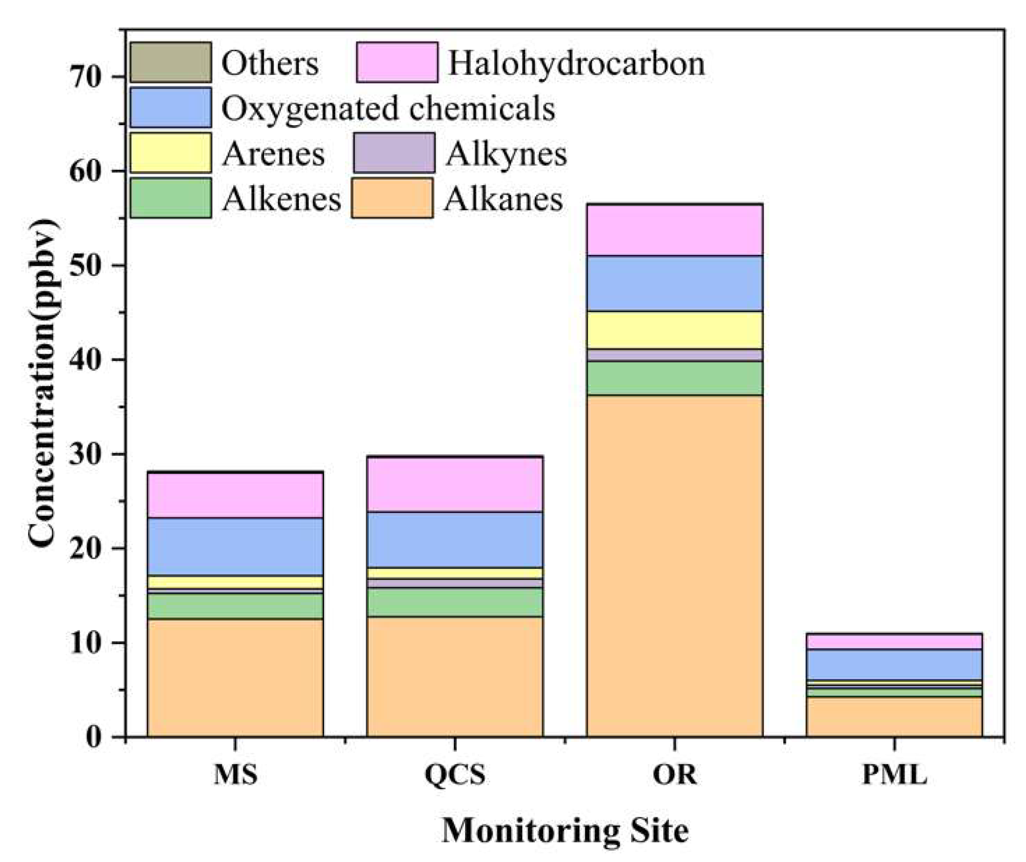
The main components of the VOCs in summer in Jinan city were alkanes, oxygenates, halogenated hydrocarbons, and olefins, accounting for 52%, 17%, 14%, and 8% of the mass concentration of TVOCs, respectively. Table 2 provides a comparison between the study of VOCs in the summer in other cities in China. The study also selected Yantai, which is a coastal city in Shandong Province, Taizhou and Shaoxing in the Yangtze River Delta region, Zhengzhou, which is an important megacity in central China, and Chengdu, which is a typical city in Chengdu–Chongqing region, as comparative references. The results show that the mass concentration of TVOCs in Jinan is close to that in Chengdu, higher than that in Yantai and Taizhou in Shandong Province, and lower than that in Shaoxing, Zhengzhou, and other cities. Part of the reason is that there were certain differences in the number of monitored species. The proportion of alkanes in Jinan (52%) was significantly higher than that in other cities; the proportion of halogenated hydrocarbons (14%) was close to Chengdu, Taizhou, Yantai, and other cities, lower than in Shaoxing and Zhengzhou. The proportion of oxygen-containing compounds (17%) was close to that of Shaoxing and Chengdu but lower than that of Yantai, Taizhou, and Zhengzhou. The mass concentration ratio of alkynes (8%) was close to that of Yantai but lower than those of Taizhou, Zhengzhou, and Chengdu.
The concentrations of the VOCs at the monitoring stations in each region are shown in Figure 4. Alkanes, oxygenated chemicals, halohydrocarbons, and alkenes were the main VOC components in Jinan. Their average proportions at the four stations were 52, 17, 14, and 8%, respectively. The proportion of alkanes in the industrial park was 64%, while in the urban areas and suburbs, it was ~40%. The monitoring site of the industrial park was affected by the characteristic pollutant discharge of the adjacent refinery and, thus, the alkane concentrations were 36.2 ppbv, which were ~3 times and 9 times the concentrations recorded at the urban and suburban sites, respectively.
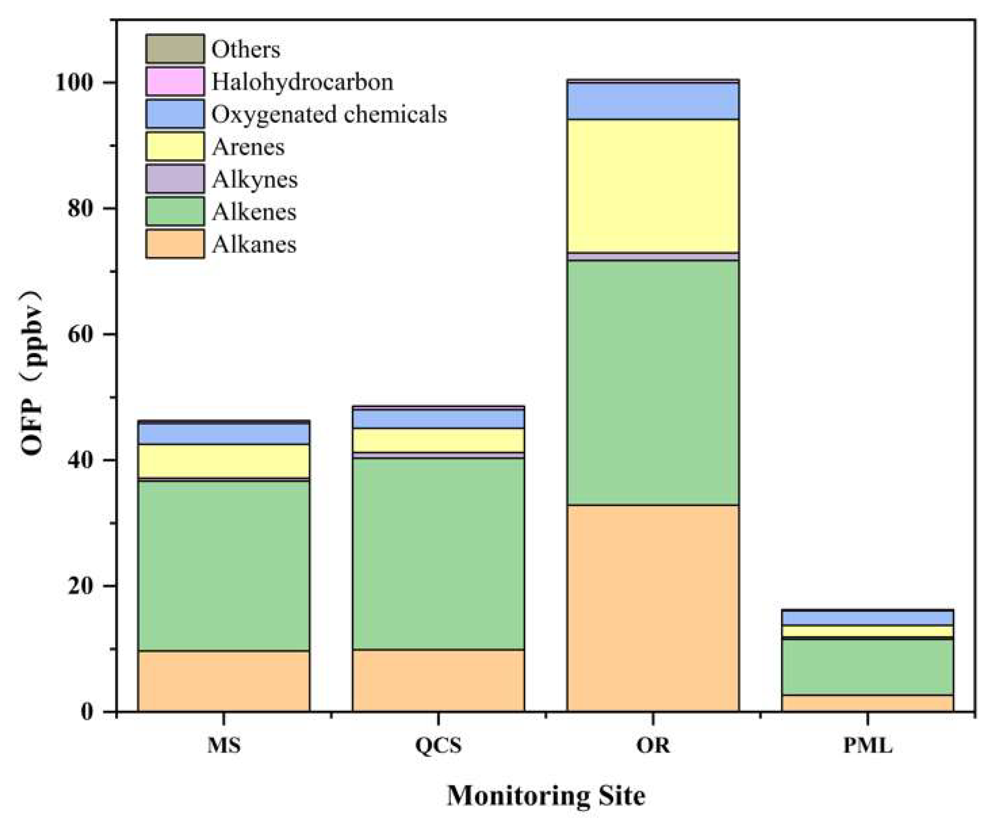
As shown in Figure 5, the industrial park site had the highest OFP (100 ppbv), which was ~2 times and 6 times that of the two sites in the urban area, respectively. The contribution of alkenes, alkanes, and arenes to the OFP value in Jinan reached ~50, 26, and 15%, respectively.
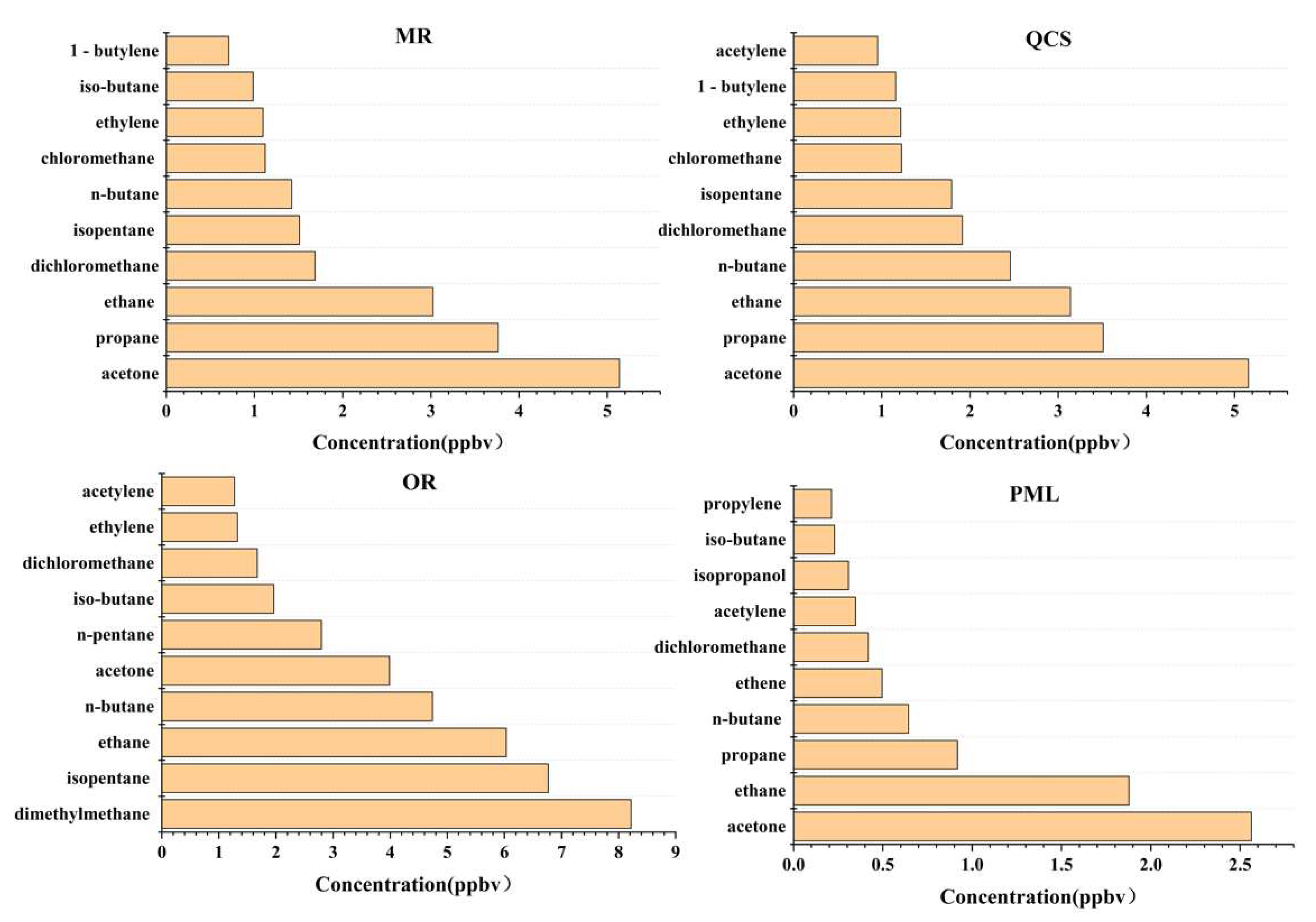
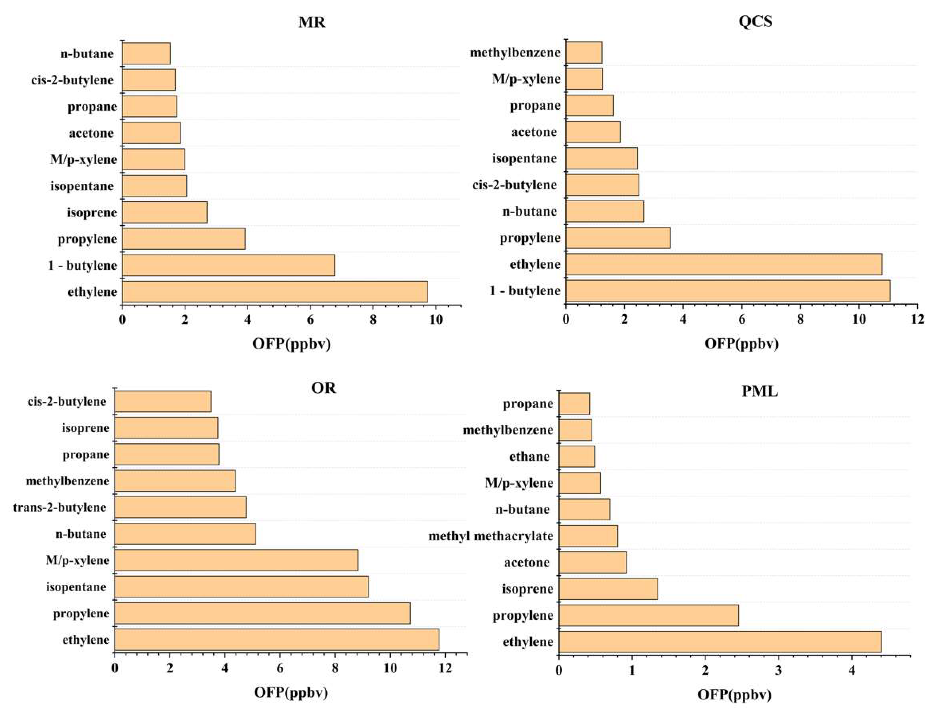
The species with the highest VOC component concentration in Jinan were mainly C2-C5-containing alkenes, acetone, dichloromethane, etc., which indicates that, on the whole, the VOCs in Jinan were obviously affected by vehicle exhaust, gasoline, LPG, and other fuels’ volatilization, industrial emissions, etc. The top species of OFP were mainly olefins and aromatic hydrocarbons with strong photochemical reaction activity (such as 1-butene, ethylene, propylene, M/p-xylene, and toluene) and alkanes with high concentrations (propane, n-butane, isopentane, etc.), mainly from vehicle exhaust, industrial production, and other emissions.
The top ten species in concentration and OFP among the four sites are shown in Figure 6 and Figure 7. Among the top 10 species ranked in terms of concentration and OFP, each site was relatively similar. Therefore, to control O3 generation, each site should start with the species with the higher OFP.
3.2. Sensitivity of O3 Formation to Precursors
3.2.1. EKMA
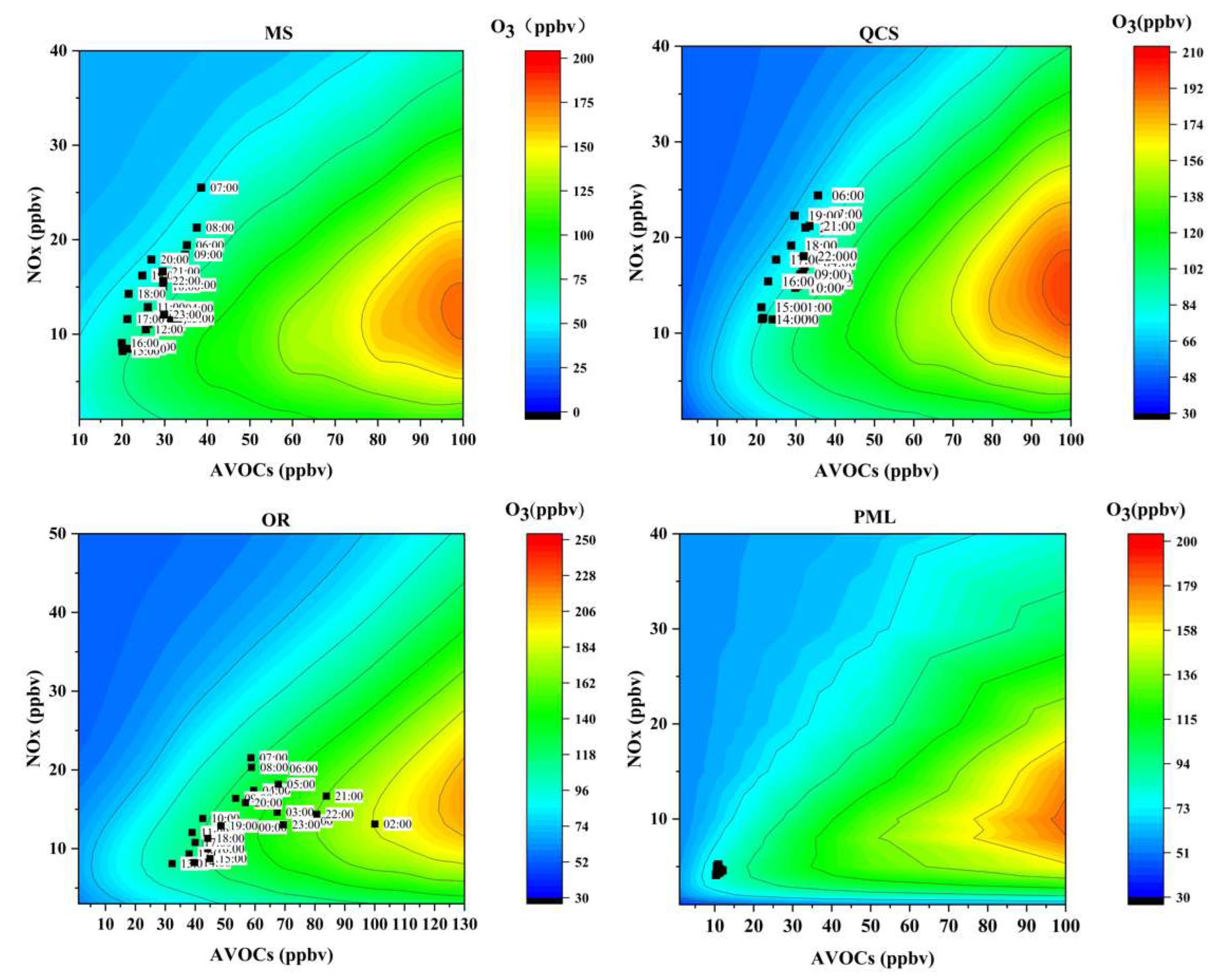
The EKMA curve was used to identify the ozone generation control area in the study area. The concentration of NOx, AVOCs, CO, and other precursors and the mean value of the meteorological condition parameters corresponding to the day when O3 exceeded the standard was used as the reference conditions for drawing the EKMA curve. We set up multiple precursor concentration combination scenarios according to the concentration of the atmospheric environmental pollutants and meteorological observation data in the study area [28]. First, we selected the concentration of the precursors (VOCs, NOx) corresponding to the baseline scenario, that is, the concentration of the VOCs and NOx in the actual observation, which can be the average value of the observation over a period of time. Then, it was assumed that different concentrations of VOCs and NOx could form multiple precursor concentration combination scenarios. The concentration combination of multiple precursors could be obtained by increasing or decreasing the concentration of NOx per hour in the time dimension in an equal proportion or by increasing or decreasing the concentration of each component of VOCs per hour in an equal proportion. The number of combined scenarios was unlimited, and the number of combined scenarios of the precursor concentration can be determined according to the actual application needs.
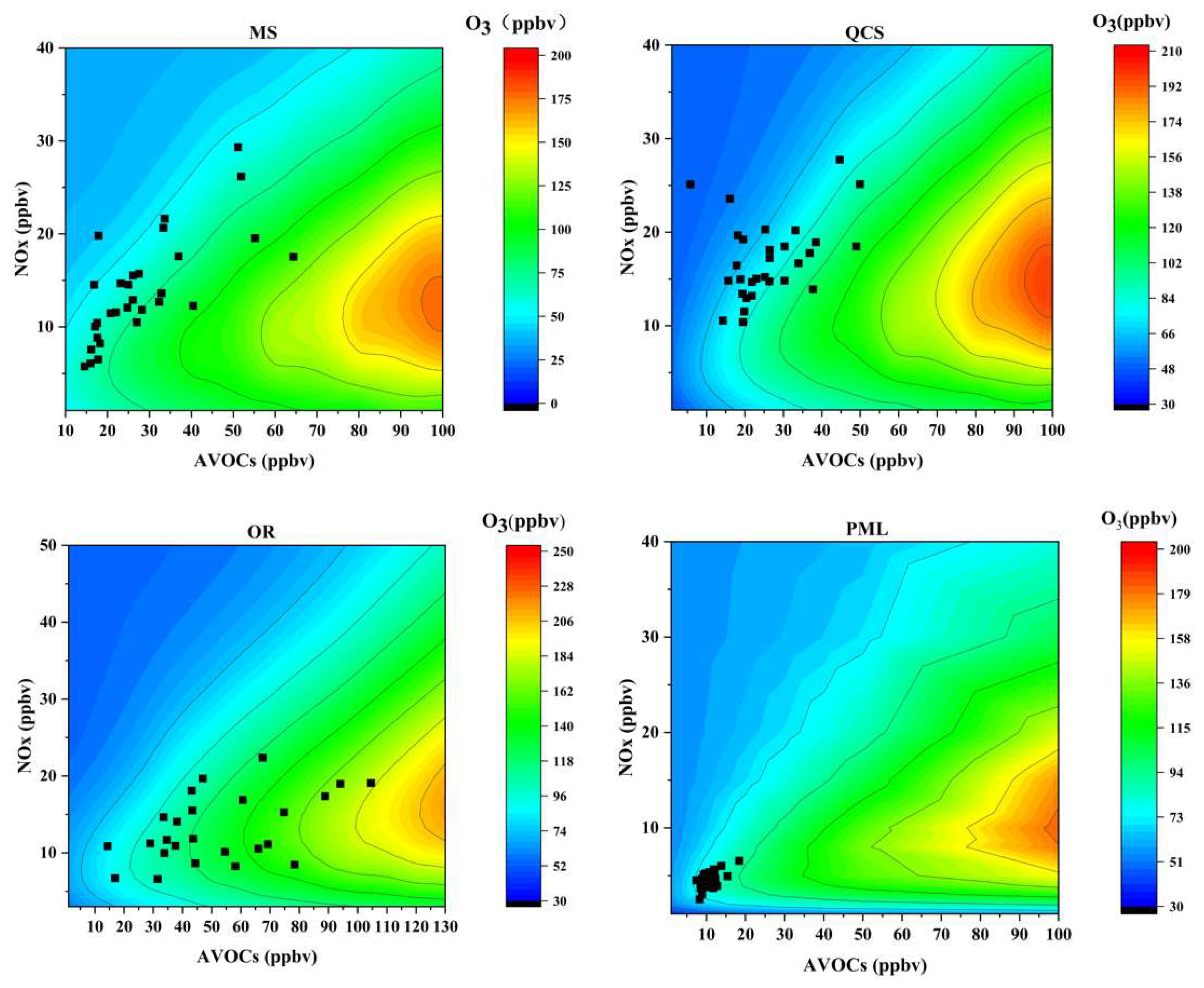
In this study, 196 monitoring scenarios were simulated, and the combined scenario of the precursor concentration was input into the box model containing an atmospheric photochemical reaction to draw the EKMA curve and to identify the ozone generation sensitive area information. The daily sensitivity (Figure 8) and hourly sensitivity (Figure 9) of ozone generation represent two different time modes. The Daily sensitivity is to process the data of VOCs and NOx into average daily concentrations and place them in the EKMA curve to determine the sensitivity of ozone generation on different days. The hourly sensitivity is to process the concentration data at the same time on different days in June to obtain the average concentration at different times of 0:00–23:00, and then placed in the EKMA curve to determine the ozone generation sensitivity at different times of the month. These two different ways are reflected in the figure: in the daily sensitivity (Figure 8), each black dot represents the average ozone concentration of each day in June; In the hourly sensitivity (Figure 9), each black dot represents the average ozone concentration of the hour. There are 24 black dots, representing 24 h.
There were certain differences in the sensitive areas of O3 generation in the different regions, as shown in Figure 8. The daily concentrations of O3 at the urban sites were mainly located above the ridge line, typical of the VOC-sensitive area. The industrial park site was in the VOCs-NOx transition zone most often, while the O3 pollution day at the suburban site was near the ridge line and was in the VOCs-NOx transition zone.
The average hourly concentrations of VOCs and NOx at each site in June were placed in the EKMA curve to analyze the O3-sensitive areas of each site in Jinan at different times in June. As shown in Figure 9, the urban and suburban sites did not change significantly during the day and night, urban sites were mainly located in the VOC-sensitive area, and the suburban site was mainly located in the VOC-NOx-sensitive area. while the industrial park site was in the VOC-sensitive area from night till morning; it was in the VOCs-NOx transition area in the afternoon.
3.2.2. RIR of the Major Precursors
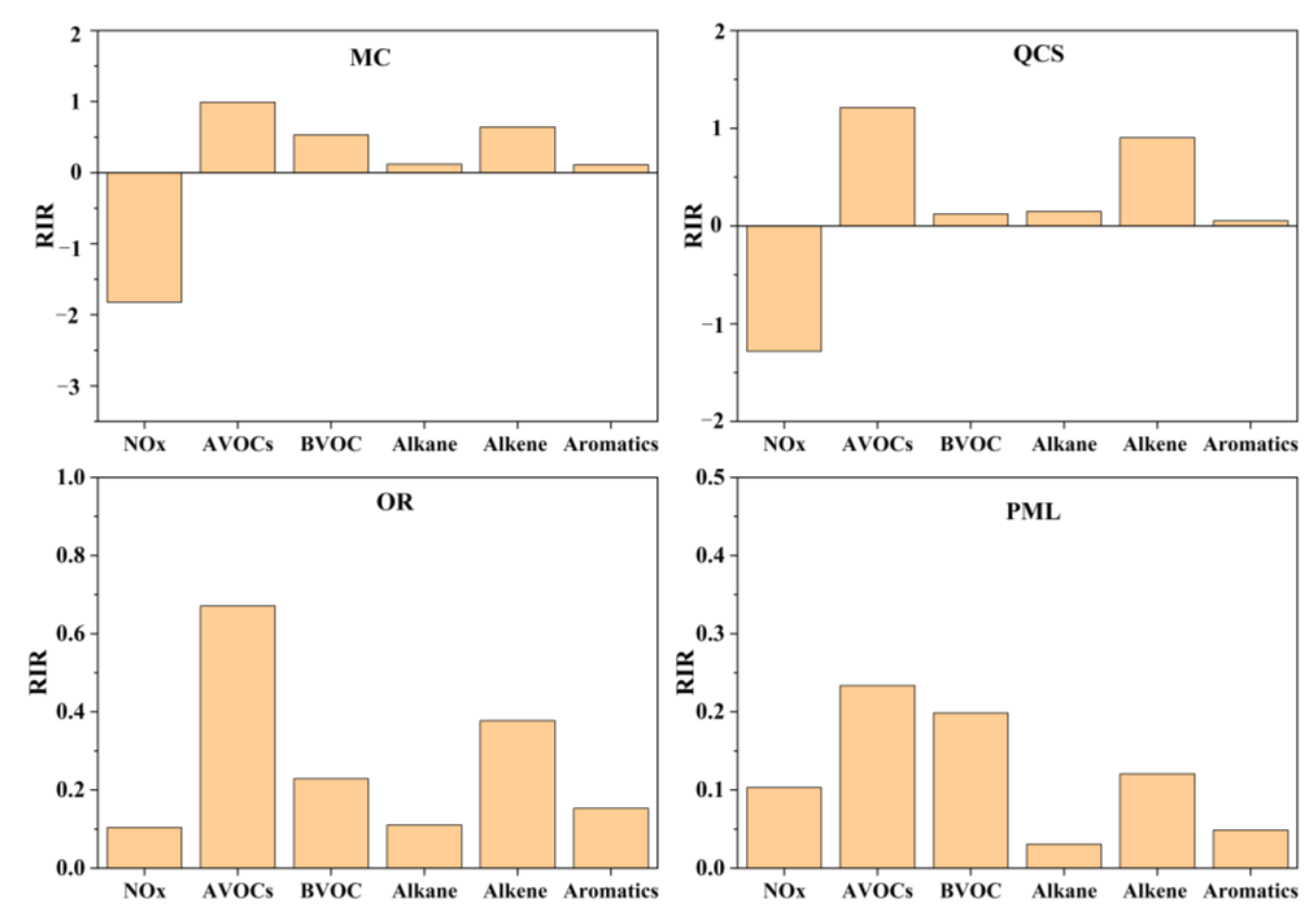
The O3 precursors were divided into NOx, anthropogenic VOCs (AVOCs), and natural VOCs (BVOCs, represented by the observed species, isoprene). The RIR values of the O3 precursors corresponding to the different sites were obtained by simulation, as shown in Figure 10. The RIR value indicates the sensitivity of the different precursors to O3. When the RIR value is greater than zero, this indicates that controlling the emission of the given precursor can reduce the generation of O3. The larger the value, the more sensitive the generation of O3 [41]. When the RIR value is less than zero, this indicates that controlling the emission of this precursor promotes the generation of O3, increasing the concentration of O3. Overall, the reduction of VOCs at each site in Jinan could reduce the concentration of O3. AVOCs were the most sensitive to O3 generation, while natural sources (isoprene) were less sensitive. NOx reduction at the industrial park sites and suburban sites also reduced the O3 concentrations. There was a strongly adverse effect of NOx reduction at the urban sites, i.e., NOx reduction alone increased the O3 concentrations instead of decreasing them. The RIR values corresponding to different types of VOCs showed that alkenes were the most sensitive to O3 generation. O3 control in Jinan city should increase the control of such VOC species in the summer.
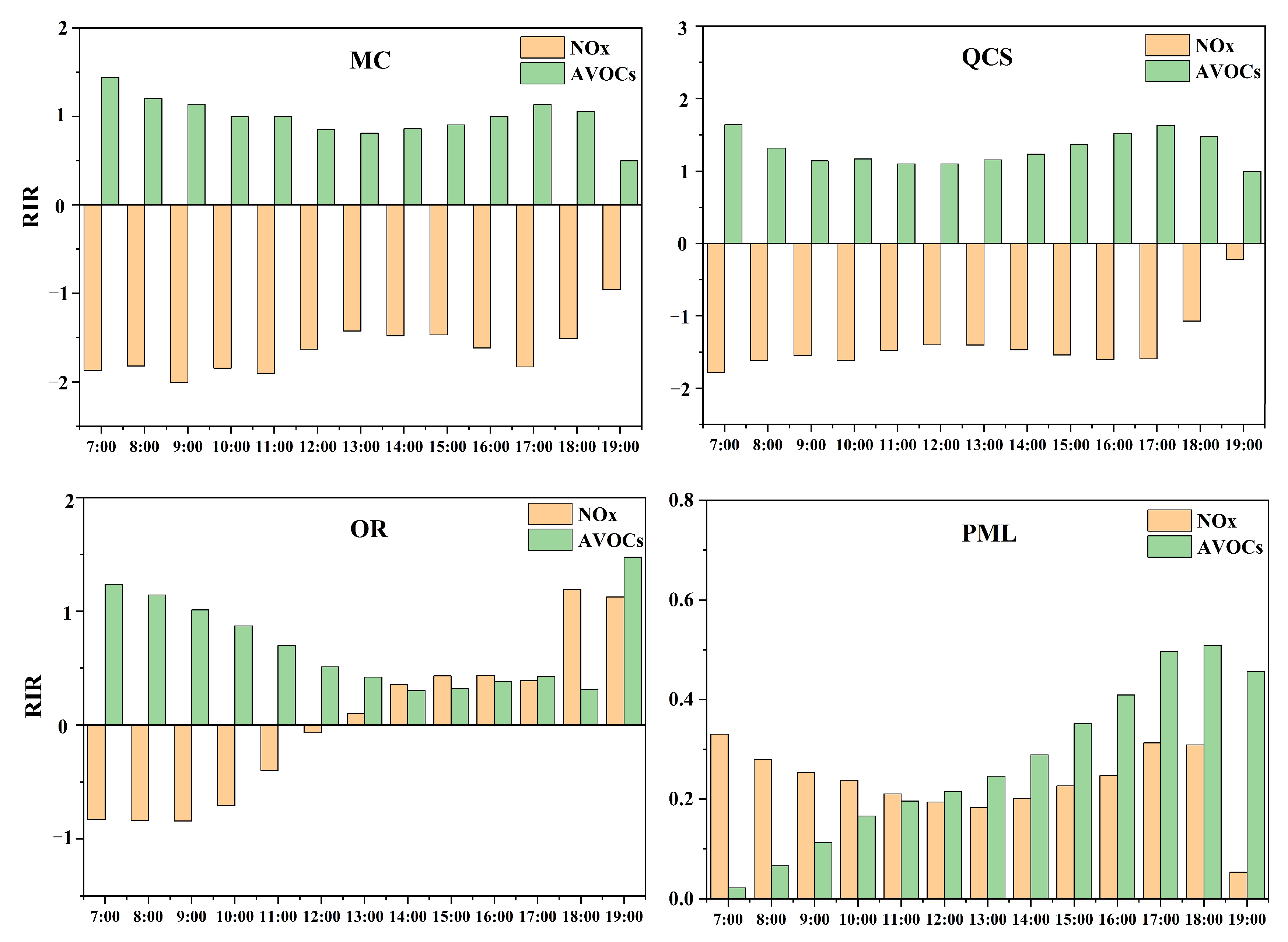
The diurnal variation in the sensitivity of the O3 precursors is shown in Figure 11. The suburban sites exhibited better NOx reduction in the morning (7:00–11:00) and better AVOCs reduction in the afternoon. In the industrial park, in the morning, due to the increase in NOx emissions from motor vehicles and industrial enterprises during work hours, the O3 generation was sensitive to AVOCs, which led to the appearance of the adverse effects of NOx. In the afternoon, with the reduction in NOx emissions, the adverse effects of NOx gradually weakened. The generation of O3 changed from being VOCs-sensitive to the VOCs-NOxtransition zone. The NOx reduction at 14:00–18:00 was more effective for a reduction in the O3 concentration. Some studies have reported that the O3 generation mechanism in key regions, such as Beijing–Tianjin–Hebei, the Pearl River Delta, and the Yangtze River Delta, in China has changed from VOC-sensitive in the morning to the transition zone in the afternoon (NOx-sensitive in the Pearl River Delta), which may be related to the photochemical consumption of NOx or its diffusion [23,42,43]. Overall, a control strategy based on VOCs in Jinan will be effective in reducing O3 concentration. It is not suitable for urban areas to reduce NOx emissions alone, while coordinated reduction of NOx emissions in industrial parks in the afternoon will be more beneficial for the reduction of O3.
3.3. VOC Source Apportionment by PMF
The sensitivity study of O3 generation in Jinan showed that cutting VOCs at each site could reduce O3 generation. Therefore, PMF was used to further analyze the source of VOCs in Jinan in June 2021. In this study, more than 40 characteristic species were selected for use as input to the model calculation.
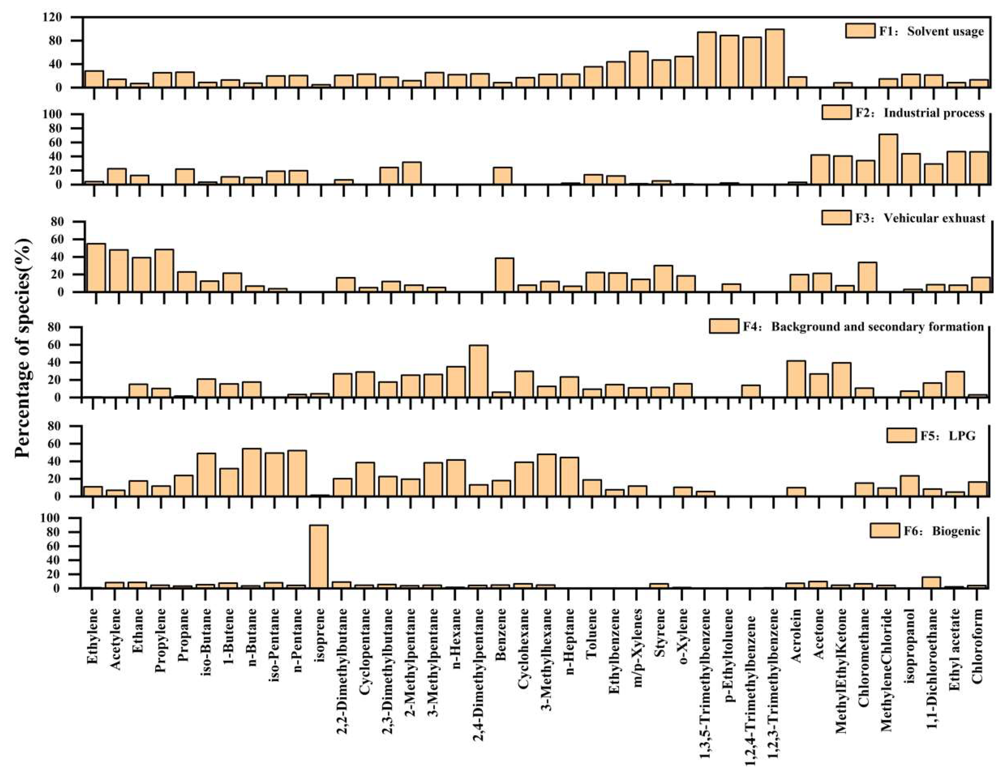
The source component spectrum of VOCs in the ambient air over the summer season was obtained by PMF source analysis and is shown in Figure 12 (taking the city monitoring station as an example). The sources of VOCs could be determined according to the contribution of representative species in the spectrum. More than half of factor 1 was associated with o-xylene, 1,3, 5-tritoluene, p-ethyl toluene, 1,2, 4-tritoluene, and 1,2, 3-tritoluene. The urban benzene series mainly originated from solvent use [44]; therefore, factor 1 was judged to be the source of the solvent use. In factor 2, methylene chloride, chloroform, acetone, 2-butanone, isopropanol, and ethyl acetate accounted for a relatively high proportion. Halogenated hydrocarbons, such as methylene chloride and chloroform, mainly originated from industrial emissions [45], while 2-butanone, isopropanol, and ethyl acetate were mainly emitted from industrial solvents, suburban agents, etc. [46]; therefore, factor 2 was associated with industrial emissions. The contribution of C2-C5 alkenes, acetylene, toluene, and benzene was relatively high toward factor 3. All of these compounds are characteristic species of vehicle exhaust [47]; therefore, factor 3 was judged as vehicle exhaust emission. Species with a high proportion of factor 4 contributions included C4-C5 alkanes emitted by motor vehicles and oxygenates emitted by industrial solvent use (acetone, 2-butanone, acrolein, and ethyl acetate). Therefore, this factor was a mixture of characteristic species from multiple sources and was judged as a local mixed source. In factor 5, C4-C5 alkanes, such as isobutane, n-butane, isopentane, n-pentane, and 2, 4-dimethyl pentane, accounted for a relatively high contribution. They were mainly LPG tracer species [44], and factor 5 was judged to be the volatile source of LPG. The contribution of isoprene to factor 6 was 89%. Isoprene was the tracer species from natural sources [48]; therefore, it was judged that this factor was emitted from natural sources.
The sources of VOCs in the ambient air of Jinan according to the PMF analysis are shown in Table 3. In the summer, VOCs in Jinan mainly originated from vehicle exhaust, the volatilization of oil and gas, industrial emissions, and solvent use. Urban vehicle exhaust and industrial emissions accounted for more than 20% of the VOCs, and solvent use accounted for ~10%. The proportion of emissions from motor vehicles, the volatilization of oil and gas, and solvents used in the industrial park was higher than that in the urban area, where the volatilization of oil and gas accounted for 23.7% of all VOCs. This is because there were oil refineries near the monitoring site in the industrial park. The proportion of natural sources, regional background, and second-generation formation of VOCs in the suburbs of Jinan city was significantly higher than that in the urban areas and industrial parks, and there was a certain amount of combustion source emissions (33.3%).
Comparing the source analysis results of Jinan with other cities in China are shown in Table 4. It was found that the emission sources of Jinan are similar to those of Wuhan. Mobile sources and industrial sources were the main sources of VOCs. Combustion sources contributed to the source of VOCs to a certain extent. Compared with other cities, the contribution of natural sources in Jinan was relatively small.
4. Conclusions
(1) The generation of O3 in the ambient air of Jinan city is in the VOC control area. Reducing NOx alone in the short term will aggravate the deterioration of ozone pollution, and a strategy for a VOCs and NOx-coordinated emissions reduction should be implemented. O3 generation in industrial parks and suburbs is in the coordinated control area of NOx and VOCs. Reducing VOCs and NOx can effectively reduce O3 concentration, and reducing VOCs had a more obvious effect on improving O3 pollution. It is worth noting that the industrial park was in an obvious VOCs-sensitive area at night and the morning and a VOCs-NOx transition area in the afternoon. The coordinated reduction of NOx emissions in the afternoon will be more beneficial to reduce O3 pollution.
(2) The main components of VOCs in the summer in Jinan city are alkanes, oxygenates, halogenated hydrocarbons, and olefins, accounting for 52%, 17%, 14%, and 8% of TVOCs’ mass concentration, respectively. The main active AVOC species in each region are olefins, followed by aromatic hydrocarbons and alkanes. The reduction of such pollutants should be strengthened.
(3) The main sources of VOCs in Jinan are motor vehicle exhaust, volatile oil and gas, industrial emissions, and solvent use, accounting for 23%, 11%, 21%, and 10%, respectively.
Author Contributions
Conceptualization, C.X. and Y.B.; methodology, C.X. and Y.B.; validation, C.X. and S.S.; formal analysis, C.X. and Y.B.; investigation, H.D.; resources, Y.B. and Z.Z.; data curation, Z.Z.; writing—original draft preparation, C.X. and X.H.; writing—review and editing, C.X. and Z.C.; visualization, C.X. and Y.B.; supervision, Y.B. All authors have read and agreed to the published version of the manuscript.
Funding
This research was funded by the National Research Program for Key Issues in Air Pollution Control (DQGG202118).
Institutional Review Board Statement
Not applicable.
Informed Consent Statement
Not applicable.
Data Availability Statement
The datasets generated and analyzed during the current study are available from the corresponding author upon reasonable request.
Acknowledgments
The authors would like to extend our deep gratitude to the reviewers and editors who provided valuable comments to improve the quality of the paper.
Conflicts of Interest
The authors declare no conflict of interest.
References
- Wang, X.; Li, J.; Zhang, Y.; Xie, S.; Tang, X. Ozone source attribution during a severe photochemical smog episode in Beijing, China. Sci. Sin. 2009, 39, 548–559. [Google Scholar] [CrossRef]
- Hao, W.; Wang, W.; Zhang, Y.; Wang, Y.; He, M. Analysis of ozone generation sensitivity in Chengdu and establishment of control strategy. Acta Sci. Circumst. 2018, 38, 3894–3899. [Google Scholar] [CrossRef]
- Liu, C.; Zhang, L.; Wen, Y.; Shi, K. Sensitivity analysis of O3 formation to its precursors-Multifractal approach. Atmos. Environ. 2021, 251, 118275–118284. [Google Scholar] [CrossRef]
- Xu, D.; Yuan, Z.; Wang, M.; Zhao, K.; Liu, X.; Duan, Y.; Fu, Q.; Wang, Q.; Jing, S.; Wang, H.; et al. Multi-factor reconciliation of discrepancies in ozone-precursor sensitivity retrieved from observation- and emission-based models. Environ. Int. 2022, 158, 106952. [Google Scholar] [CrossRef] [PubMed]
- Bell, M.; McDermott, A.; Zeger, S.; Samet, J.; Dominici, F. Ozone and short-term mortality in 95 US urban communities, 1987–2000. JAMA 2004, 292, 2372–2378. [Google Scholar] [CrossRef] [Green Version]
- Ashmore, M. Assessing the future global impacts of ozone on vegetation. Plant Cell Environ. 2005, 28, 949–964. [Google Scholar] [CrossRef]
- Ainsworth, E.A. Understanding and improving global crop response to ozone pollution. Plant J. 2017, 90, 886–897. [Google Scholar] [CrossRef]
- Li, Y.; Yin, S.; Yu, S.; Bai, L.; Wang, X.; Lu, X.; Ma, S. Characteristics of ozone pollution and the sensitivity to precursors during early summer in central plain, China. J. Environ. Sci. 2021, 99, 354–368. [Google Scholar] [CrossRef]
- Wang, Y.; Guo, H.; Zou, S.; Lyu, X.; Ling, Z.; Cheng, H.; Zeren, Y. Surface O3 photochemistry over the South China Sea: Application of a near-explicit chemical mechanism box model. Environ. Pollut. 2018, 234, 155–166. [Google Scholar] [CrossRef]
- Derwent, R.; Jenkin, M.; Saunders, S. Photochemical ozone creation potentials for a large number of reactive hydrocarbons under European conditions. Atmos. Environ. 1996, 30, 181–199. [Google Scholar] [CrossRef]
- Jia, L.; Ge, M.; Xu, Y.; Du, L.; Zhuang, G.; Wang, D. Advances in Atmospheric Ozone Chemistry. Prog. Chem. 2006, 18, 1565–1574. [Google Scholar]
- Wu, W.; Xue, W.; Lei, Y.; Wang, J. Sensitivity analysis of ozone in Beijing-Tianjin-Hebei (BTH) and its surrounding area using OMI satellite remote sensing. China Environ. Sci. 2018, 38, 1201–1208. [Google Scholar] [CrossRef]
- Wang, T.; Ding, A.; Gao, J.; Wu, W. Strong ozone production in urban plumes from Beijing, China. Geophys. Res. Lett. 2006, 33, L21806. [Google Scholar] [CrossRef] [Green Version]
- An, J.; Wang, Y.; Li, X.; Sun, Y.; Shen, S.; Shi, L. Analysis of the Relationship between NO, NO2 and O3 Concentrations in Beijing. Environ. Sci. 2007, 28, 706–711. [Google Scholar] [CrossRef]
- Liu, J.; Wu, D.; Fan, S.; Liao, Z.; Deng, T. Impacts of precursors and meteorological factors on ozone pollution in Pearl River Delta. China Environ. Sci. 2017, 37, 813–820. [Google Scholar]
- Ren, J.; Zhu, K.; Xie, M.; Liu, W.; Gao, D.; Chen, J.; Jin, Y.; Zhao, R.; Zhang, L. Analysis of the ozone sensitivity and source appointment in Xianning, Hubei Province. China Environ. Sci. 2021, 41, 4060–4068. [Google Scholar] [CrossRef]
- Lin, Y.; Duan, Y.; Gao, Z.; Lin, C.; Zhou, S.; Song, Z.; Chen, X.; Liang, G.; Wang, Q.; Huang, K.; et al. Typical ozone pollution process and source identification in Shanghai based on VOCs intense measurement. Acta Sci. Circumst. 2019, 39, 126–133. [Google Scholar] [CrossRef]
- Liang, Y.; Yin, K.; Hu, Y.; Liu, B.; Liao, N.; Yan, M. Sensitivity analysis of ozone precursor emission in Shenzhen, China. China Environ. Sci. 2014, 34, 1390–1396. [Google Scholar]
- Yang, X.; Tang, L.; Zhang, Y.; Mu, Y.; Wang, M.; Chen, W.; Zhou, H.; Hua, Y.; Jiang, R. Correlation Analysis Between Characteristics of VOCs and Ozone Formation Potential in Summer in Nanjing Urban District. Environ. Sci. 2016, 37, 443–451. [Google Scholar] [CrossRef]
- Jin, X.; Holloway, T. Spatial and temporal variability of ozone sensitivity over China observed from the Ozone Monitoring Instrument. J. Geophys. Res. Atmos. 2015, 120, 7229–7246. [Google Scholar] [CrossRef]
- Wang, T.; Xue, L.; Brimblecombe, P.; Lam, Y.; Li, L.; Zhang, L. Ozone pollution in China: A review of concentrations, meteorological influences, chemical precursors, and effects. Sci. Total Environ. 2017, 575, 1582–1596. [Google Scholar] [CrossRef] [PubMed]
- Lu, K.; Zhang, Y.; Su, H.; Brauers, T.; Chou, C.; Hofzumahaus, A.; Liu, S.; Kita, K.; Kondo, Y.; Shao, M.; et al. Oxidant (O3 + NO2) production processes and formation regimes in Beijing. J. Geophys. Res. 2010, 115, D07303. [Google Scholar] [CrossRef] [Green Version]
- Wang, N.; Lyu, X.; Deng, X.; Huang, X.; Jiang, F.; Ding, A. Aggravating O3 pollution due to NOx emission control in eastern China. Sci. Total Environ. 2019, 677, 732–744. [Google Scholar] [CrossRef] [PubMed]
- Ran, L.; Zhao, C.S.; Xu, W.Y.; Han, M.; Lu, X.Q.; Han, S.Q.; Lin, W.L.; Xu, X.B.; Gao, W.; Yu, Q.; et al. Ozone production in summer in the megacities of Tianjin and Shanghai, China: A comparative study. Atmos. Chem. Phys. 2012, 12, 7531–7542. [Google Scholar] [CrossRef] [Green Version]
- Li, K.; Wang, X.; Li, L.; Wang, J.; Liu, Y.; Cheng, X.; Xu, B.; Wang, X.; Yan, P.; Li, S.; et al. Large variability of O3-precursor relationship during severe ozone polluted period in an industry-driven cluster city (Zibo) of North China Plain. J. Clean. Prod. 2021, 316, 128252–128267. [Google Scholar] [CrossRef]
- Tang, X.; Zhang, Y.; Shao, M. Atmospheric Environmental Chemistry; Higher Education Press: Beijing, China, 2006. [Google Scholar]
- Sun, X.; Zhao, M.; Shen, H.; Liu, Y.; Du, M.; Zhang, W.; Xu, H.; Fan, G.; Gong, H.; Li, Q.; et al. Ozone Formation and Key VOCs of a Continuous Summertime O3 Pollution Event in Ji’nan. Environ. Sci. 2022, 43, 686–695. [Google Scholar] [CrossRef]
- Carter, W.P.L. Development of ozone reactivity scales for volatile organic-compounds. J. Air Waste Manag. Assoc. 1994, 44, 881–899. [Google Scholar] [CrossRef] [Green Version]
- Yu, D.; Tan, Z.; Lu, K.; Ma, X.; Li, X.; Chen, S.; Zhu, B.; Lin, L.; Li, Y.; Qiu, P.; et al. An explicit study of local ozone budget and NOx-VOCs sensitivity in Shenzhen China. Atmos. Environ. 2020, 224, 117304–117317. [Google Scholar] [CrossRef]
- China MoEPotPsRo. Pilot Study on Source Analysis Technology of Ambient Air Ozone Pollution. Available online: https://www.mee.gov.cn/xxgk2018/xxgk/xxgk06/201807/W020180926550435480461.pdf (accessed on 1 June 2022).
- Liu, C.; Shi, K. A review on methodology in O3-NOx-VOC sensitivity study. Environ. Pollut. 2021, 291, 118249. [Google Scholar] [CrossRef]
- Tan, Z.; Lu, K.; Jiang, M.; Su, R.; Dong, H.; Zeng, L.; Xie, S.; Tan, Q.; Zhang, Y. Exploring ozone pollution in Chengdu, southwestern China: A case study from radical chemistry to O3-VOC-NOx sensitivity. Sci. Total Environ. 2018, 636, 775–786. [Google Scholar] [CrossRef]
- Lu, K.; Zhang, Y.; Su, H.; Shao, M.; Zeng, L.; Zhong, L.; Xiang, Y.; Zhang, Z.; Zhou, C.; Wahner, A. Regional ozone pollution and key controlling factors of photochemical ozone production in Pearl River Delta during summer time. Sci. Sin. 2010, 40, 407–420. [Google Scholar] [CrossRef]
- Zhang, J.; Wu, Y.; Li, H.; Ling, D.; Han, K.; Li, J.; Hu, J.; Wang, H.; Zhang, M.; Wang, S. Characteristics and source apportionment of ambient volatile organic compounds in autumn in Langfang development zones. China Environ. Sci. 2019, 39, 3186–3192. [Google Scholar] [CrossRef]
- Li, C.; Liu, Y.; Cheng, B.; Zhang, Y.; Liu, X.; Qu, Y.; An, J.; Kong, L.; Zhang, Y.; Zhang, C.; et al. A comprehensive investigation on volatile organic compounds (VOCs) in 2018 in Beijing, China: Characteristics, sources and behaviours in response to O3 formation. Sci. Total Environ. 2022, 806, 150247–150258. [Google Scholar] [CrossRef]
- Wang, M.; Wang, X.; Li, B.; Yi, Q. Analysis of VOCs pollution characteristics and ozone generation potential in Yantai. Environ. Sci. Technol. 2021, 44, 210–216. [Google Scholar] [CrossRef]
- Li, J.; Sun, S.; Jiang, X.; Zhang, Y.; Yu, B.; Wang, T. Characteristics, sources and atmospheric reactivity of volatile organic compounds in Shaoxing city in summer. Environ. Pollut. Control 2020, 42, 1145–1148+1170. [Google Scholar] [CrossRef]
- Fan, F.; Song, K.; Yu, Y.; Wan, Z.; Lu, S.; Tang, R.; Chen, S.; Zeng, S.; Guo, S. Chemical composition characteristics, activity and source analysis of atmospheric volatile organic compounds in Taizhou. J. Nanjing Univ. Inf. Sci. Technol. 2020, 12, 695–704. [Google Scholar] [CrossRef]
- Yu, S.; Zhang, Y.; Guo, W.; Li, Y.; Zhang, R. Pollution characteristics and source analysis of atmospheric volatile organic compounds in Zhengzhou in summer. In Proceedings of the Annual Conference of Science and Technology of Chinese Society of Environmental Sciences, Nanjing, China, 21 September 2020; pp. 4404–4410. [Google Scholar]
- Xu, C.; Chen, J.; Han, L.; Wang, B.; Wang, J. Characteristics of atmospheric VOCs pollution, ozone generation potential and source analysis in Chengdu in summer of 2017. Res. Environ. Sci. 2019, 32, 619–626. [Google Scholar] [CrossRef]
- Qian, J.; Xu, C.; Chen, J.; Jiang, T.; Han, L.; Wang, C.; Li, Y.; Wang, B.; Liu, Z. Chemical Characteristics and Contaminant Sensitivity During the Typical Ozone Pollution Processes of Chengdu in 2020. Environ. Sci. 2021, 42, 5736–5746. [Google Scholar] [CrossRef]
- Kleinman, L.I. The dependence of tropospheric ozone production rate on ozone precursors. Atmos. Environ. 2005, 39, 575–586. [Google Scholar] [CrossRef]
- Sillman, S.; West, J.J. Reactive nitrogen in Mexico City and its relation to ozone precursor sensitivity: Results from photochemical models. Atmos. Chem. Phys. 2009, 9, 3477–3489. [Google Scholar] [CrossRef] [Green Version]
- Liu, Y.; Shao, M.; Fu, L.; Lu, S.; Zeng, L.; Tang, D. Source profiles of volatile organic compounds (VOCs) measured in China: Part I. Atmos. Environ. 2008, 42, 6247–6260. [Google Scholar] [CrossRef]
- Zou, Q.; Sun, X.; Tian, X.; Tang, Q.; Song, Q.; Xu, D.; Jin, L. Ozone Formation Potential and Sources Apportionment of Atmospheric VOCs during Typical Periods in Summer of Jiashan. Environ. Monit. China 2017, 33, 91–98. [Google Scholar] [CrossRef]
- Zhang, L.; Wu, Z.; Li, B.; Liu, K.; Yue, T.; Zhang, Y. Pollution Characterizations of Atmospheric Volatile Organic Compounds in Spring of Beijing Urban Area. Res. Environ. Sci. 2020, 33, 526–535. [Google Scholar] [CrossRef]
- Wu, F.; Wang, Y.; An, J.; Zhang, J. Study on ConcentrationOzone Production Potential and Sources of VOCs in the Atmosphere of Beijing During Olympics Period. Environ. Sci. 2010, 31, 10–16. [Google Scholar] [CrossRef]
- Shao, M.; Fu, L.; Liu, Y.; Lu, S.; Zhang, Y.; Tang, X. Major reactive species of ambient volatile organic compounds (VOCs) and their sources in Beijing. Sci. China Ser. D Earth Sci. 2005, 48, 147–154. [Google Scholar]
- Xu, C.; Chen, J.; Jiang, T.; Han, L.; Wang, B.; Li, Y.; Wang, C.; Liu, Z.; Qian, J. Characteristics and Sources of Atmospheric Volatile Organic Compounds Pollution in Summer in Chengdu. Environ. Sci. 2020, 41, 5316–5324. [Google Scholar] [CrossRef]
- Ma, J.; Yan, Y.; Kong, S.; Song, A.; Chen, N.; Zhu, B.; Quan, J.; Qi, S. Characteristics and sources of ozone and its precursors around the Wuhan Military Games. China Environ. Sci. 2022, 42, 3023–3032. [Google Scholar] [CrossRef]
- Zhang, H.; Liu, M.; Wang, X.; Yang, S.; Li, Y.; Luo, L. Characteristics and sources of atmospheric VOCs during spring of 2021 in Nanchang. China Environ. Sci. 2022, 42, 1040–1047. [Google Scholar]
Figure 1.
A map of Jinan showing the location of the air quality monitoring stations.

Figure 2.
Hourly sequence diagram of meteorological parameters and the pollutant volume fraction at each station over the observation period.
Figure 2.
Hourly sequence diagram of meteorological parameters and the pollutant volume fraction at each station over the observation period.

Figure 3.
Average diurnal variation in the pollutant volume fractions at each site during the observation period.
Figure 3.
Average diurnal variation in the pollutant volume fractions at each site during the observation period.

Figure 4.
Volume fraction of volatile organic compounds at each site during the observations.

Figure 5.
Ozone formation potential (OFP) values at each point during the observation.

Figure 6.
Top 10 volatile organic compounds by volume fraction at each site.

Figure 7.
Top 10 volatile organic carbon by ozone formation potential rankings at each site.

Figure 8.
Empirical kinetics modeling approach curves for each site during the observation period. (The black dots represent the location of the daily average volume fraction of the VOCs and NOx during the observation period).
Figure 8.
Empirical kinetics modeling approach curves for each site during the observation period. (The black dots represent the location of the daily average volume fraction of the VOCs and NOx during the observation period).

Figure 9.
Empirical kinetics modeling approach curves for each site during the observation period. (The black dots represent the location of the daily hourly average volume fraction of VOCs and NOx over the observation period).
Figure 9.
Empirical kinetics modeling approach curves for each site during the observation period. (The black dots represent the location of the daily hourly average volume fraction of VOCs and NOx over the observation period).

Figure 10.
Relative incremental reactivity value (RIR) of the ozone precursors at each site.

Figure 11.
Relative incremental reactivity value (RIR) of ozone precursors at different times at each site.
Figure 11.
Relative incremental reactivity value (RIR) of ozone precursors at different times at each site.

Figure 12.
The analysis spectrum of the positive matrix factorization source analysis at the monitoring center site in June.
Figure 12.
The analysis spectrum of the positive matrix factorization source analysis at the monitoring center site in June.


Table 1.
Mean values of meteorological parameters and pollutant volume fractions at each site in June 2021.
Table 1.
Mean values of meteorological parameters and pollutant volume fractions at each site in June 2021.
| Parameter | MS | QCS | OR | PML | Average |
|---|---|---|---|---|---|
| Temperature/°C | 28.5 | 28.9 | 28.7 | 22.4 | 27.1 |
| RH/% | 46.5 | 55.0 | 55.1 | 66.9 | 55.9 |
| Pressure/hPa | 995.0 | 999.2 | 996.4 | 910.8 | 975.4 |
| O3/ppbv | 114.8 | 114.7 | 118.1 | 92.3 | 110.0 |
| NO2/ppbv | 10.8 | 14.0 | 11.6 | 3.7 | 10.0 |
| NO/ppbv | 3.2 | 3.1 | 2.4 | 0.98 | 2.4 |
| NOx/ppbv | 14.0 | 17.1 | 13.9 | 4.6 | 12.4 |
| CO/ppmv | 0.84 | 0.82 | 1.3 | 0.88 | 1.0 |
| Isoprene/ppbv | 0.25 | 0.08 | 0.33 | 0.13 | 0.21 |
| AVOCs/ppbv | 28.3 | 29.7 | 56.9 | 10.9 | 31.2 |
Table 2.
Comparison of the VOC components in Jinan and other cities.
| City | TVOCs (ppbv) | Alkane (%) | Halogenated Hydrocarbons (%) | OVOCs (%) | Arene (%) | Olefins (%) |
|---|---|---|---|---|---|---|
| Jinan (2021) | 31.4 | 52 | 14 | 17 | - | 8 |
| Yantai [36] | 27.7 | 35.4 | 15.5 | 33.1 | 6.7 | 8.2 |
| Shaoxing [37] | 77.4 | 31.4 | 22.2 | 19 | 20.5 | 6.9 |
| Taizhou [38] | 26.1 | 34.9 | 13.3 | 24.2 | 9.53 | 11.3 |
| Zhengzhou [39] | 40.5 | 24.7 | 18.7 | 34.1 | 10.7 | 10.2 |
| Chengdu [40] | 31.9 | 37.4 | 14.6 | 14.4 | 16.3 | 17.4 |
Table 3.
Results of the volatile organic carbon source analysis by positive matrix factorization.
| Monitoring Site | Vehicular Exhaust | LPG | Industrial Process | Solvent Usage | Biogenic | Background and Secondary Formation | Fuel Usage |
|---|---|---|---|---|---|---|---|
| MR | 21.7% | 19.1% | 26.0% | 12.9% | 6.9% | 13.4% | / |
| QCS | 24.5% | / | 27.3% | 13.0% | 2.5% | 20.2% | 12.5% |
| OR | 29.7% | 23.7% | 16.9% | 14.0% | 2.9% | 12.7% | / |
| PML | 16.5% | / | 12.6% | / | 8.4% | 29.1% | 33.3% |
Publisher’s Note: MDPI stays neutral with regard to jurisdictional claims in published maps and institutional affiliations. |
© 2022 by the authors. Licensee MDPI, Basel, Switzerland. This article is an open access article distributed under the terms and conditions of the Creative Commons Attribution (CC BY) license (https://creativecommons.org/licenses/by/4.0/).
Share and Cite
MDPI and ACS Style
Xu, C.; He, X.; Sun, S.; Bo, Y.; Cui, Z.; Zhang, Z.; Dong, H. Sensitivity of Ozone Formation in Summer in Jinan Using Observation-Based Model. Atmosphere 2022, 13, 2024. https://doi.org/10.3390/atmos13122024
AMA Style
Xu C, He X, Sun S, Bo Y, Cui Z, Zhang Z, Dong H. Sensitivity of Ozone Formation in Summer in Jinan Using Observation-Based Model. Atmosphere. 2022; 13(12):2024. https://doi.org/10.3390/atmos13122024
Chicago/Turabian StyleXu, Chenxi, Xuejuan He, Shida Sun, Yu Bo, Zeqi Cui, Zhanchao Zhang, and Hui Dong. 2022. "Sensitivity of Ozone Formation in Summer in Jinan Using Observation-Based Model" Atmosphere 13, no. 12: 2024. https://doi.org/10.3390/atmos13122024
Note that from the first issue of 2016, this journal uses article numbers instead of page numbers. See further details here.