
Analysis of Extreme Rainfall and Natural Disasters Events Using Satellite Precipitation Products in Different Regions of Brazil
 , ,
, ,  , , and
Abstract
:1. Introduction
2. Materials and Methods
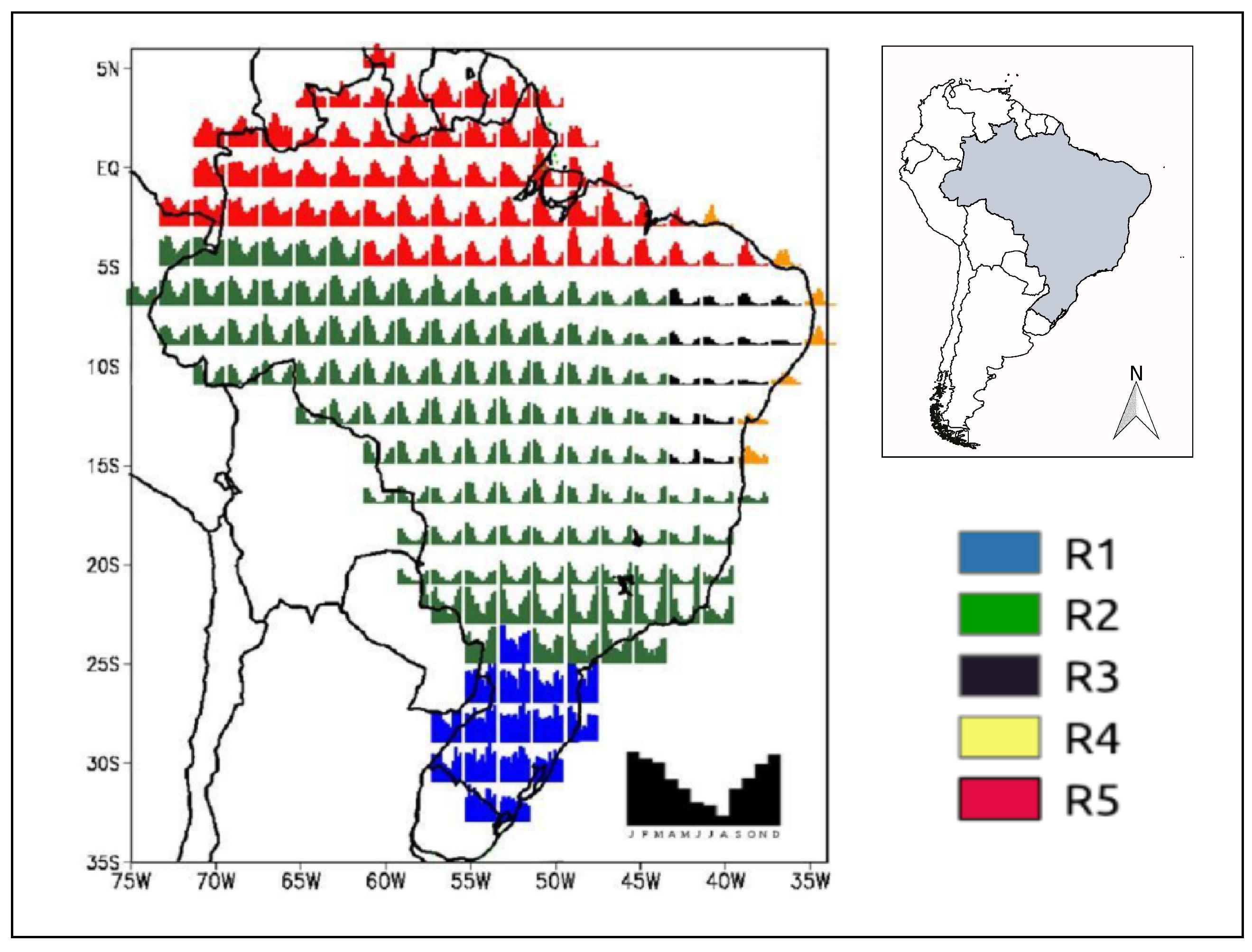
2.1. Study Area
2.2. Rain Gauges Dataset
2.3. Satellite Precipitation Products (SPP)
2.4. TOOCAN Dataset
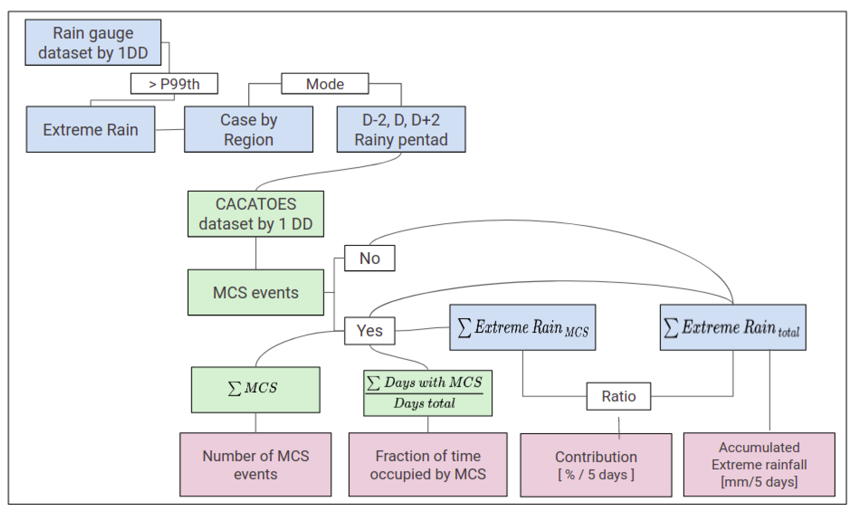
2.5. Methodology
3. Results and Discussion
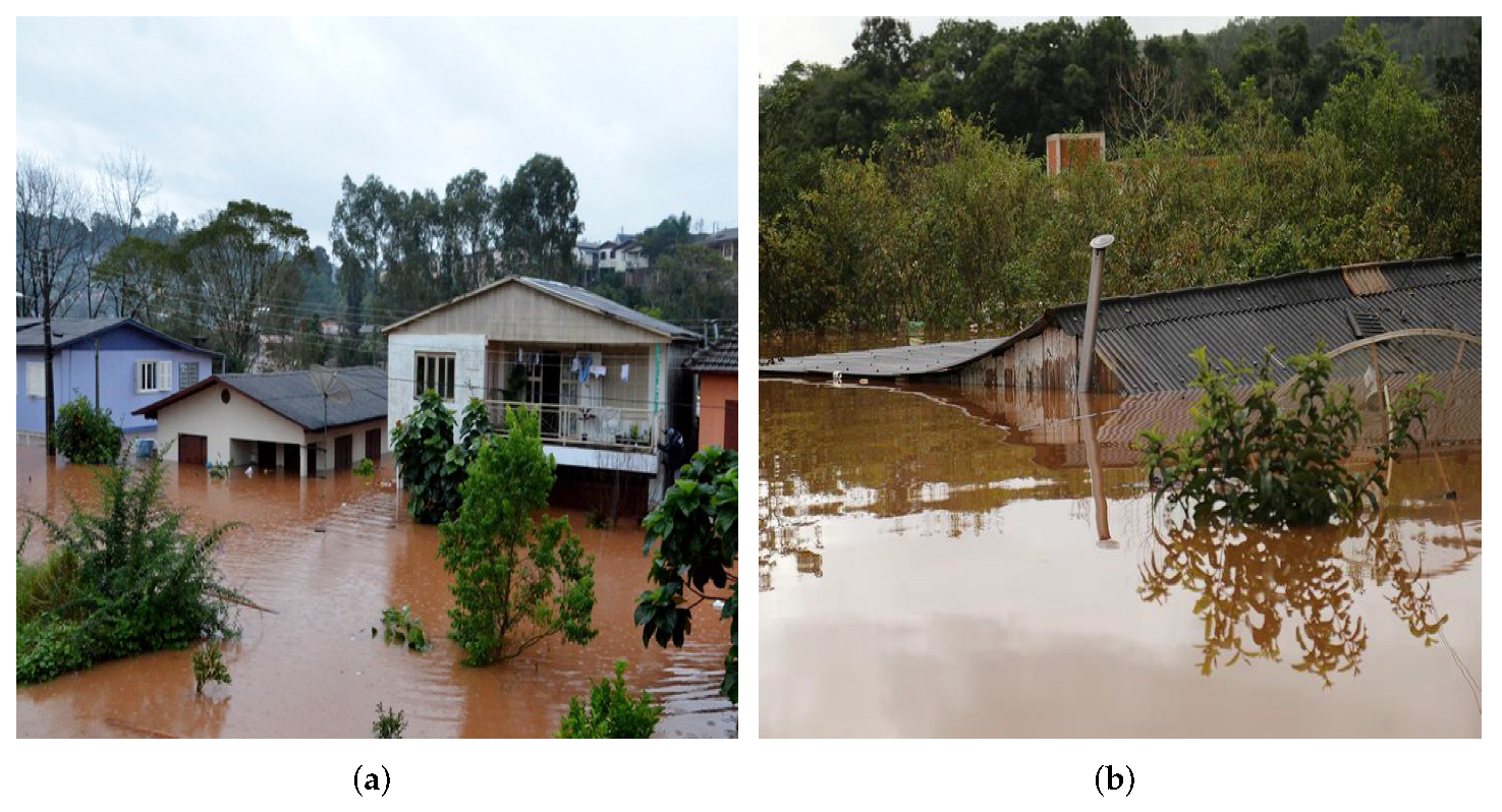
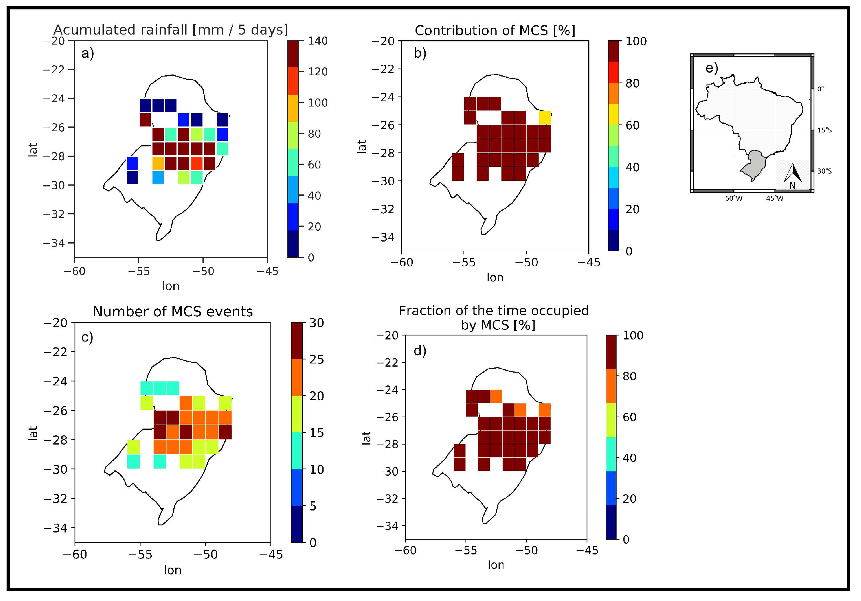
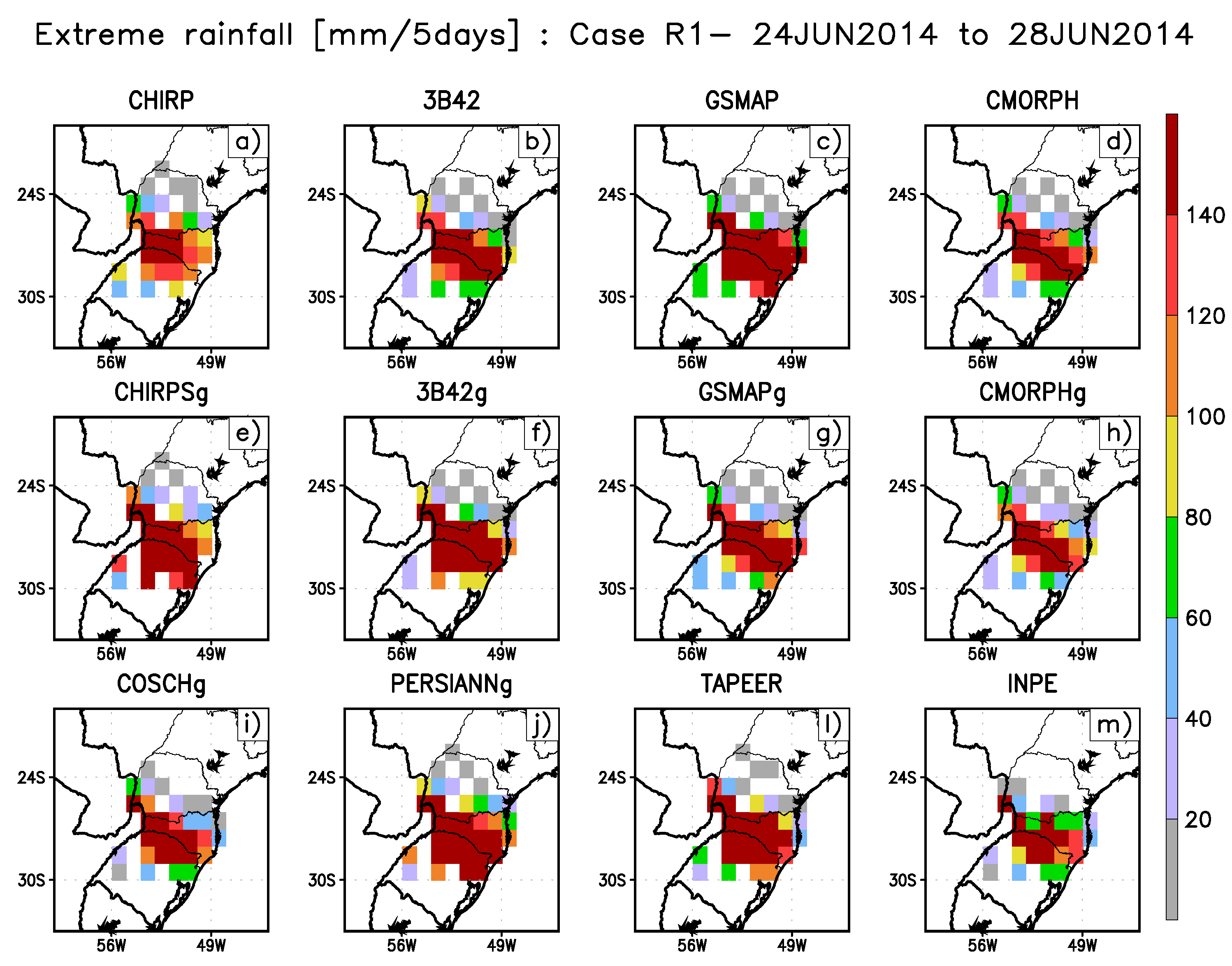
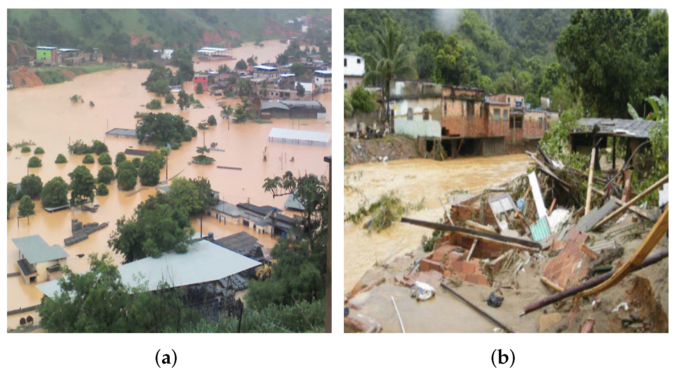
3.1. Case Study for Southern Brazil—R1
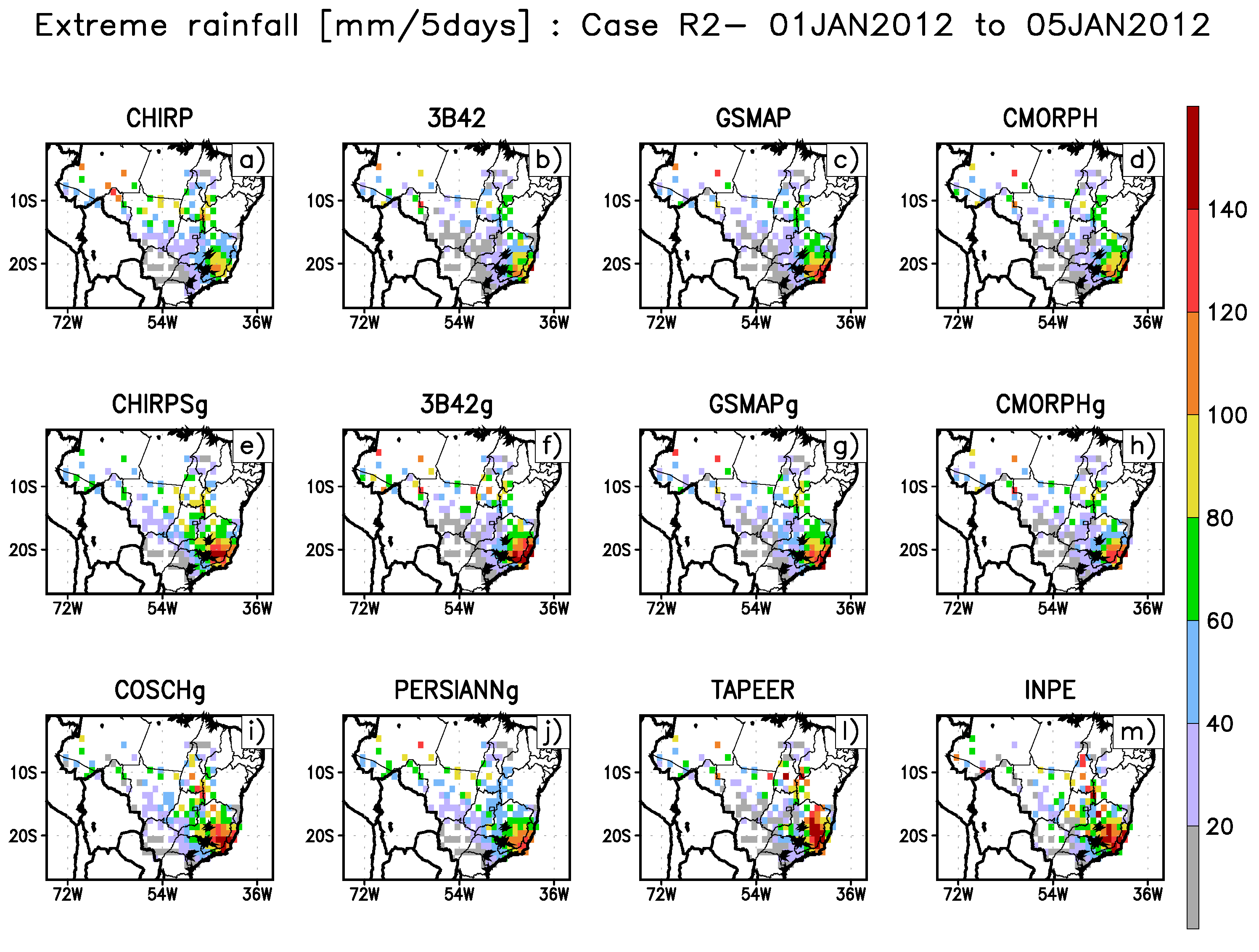
3.2. Case Study for the Central Region—R2
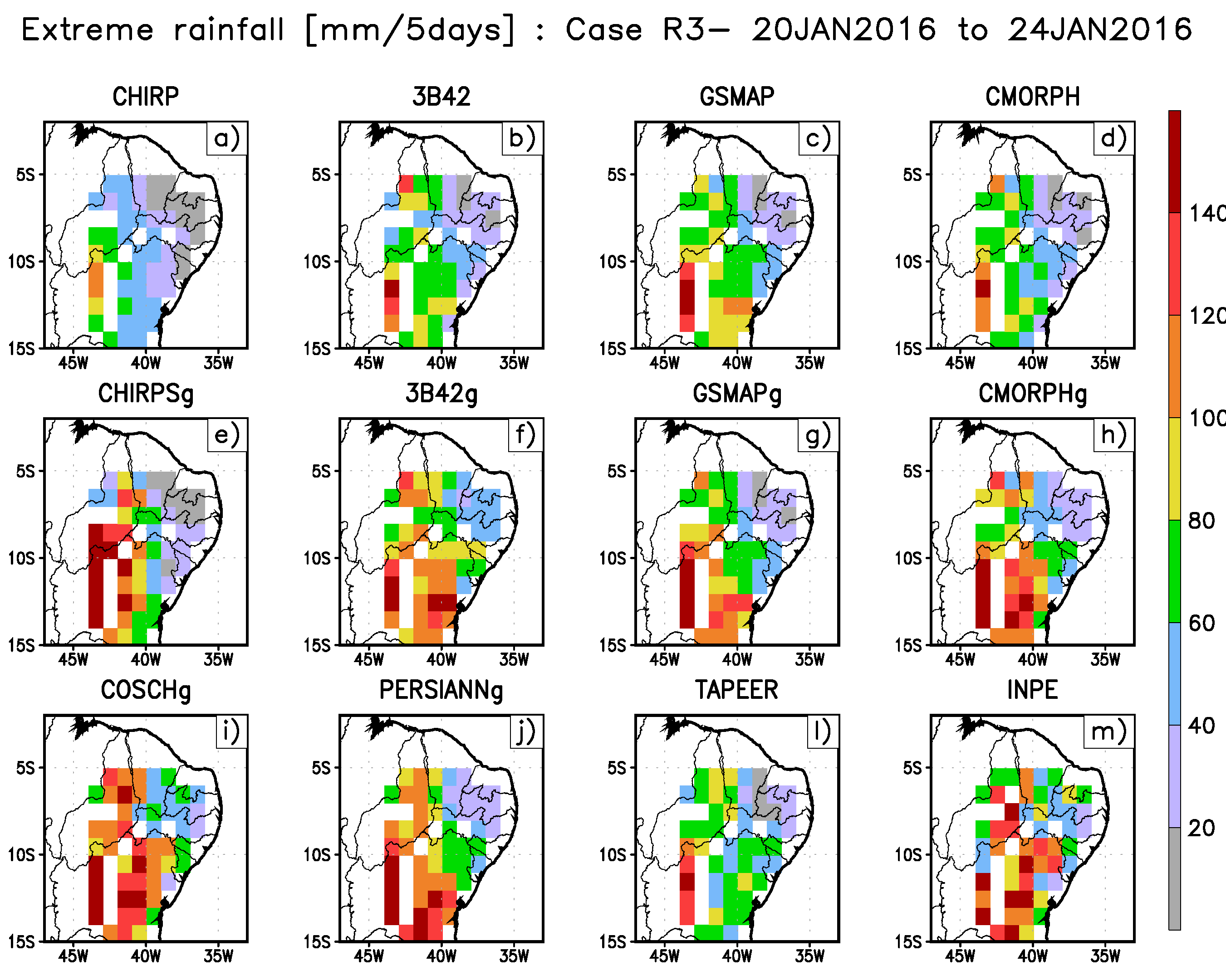
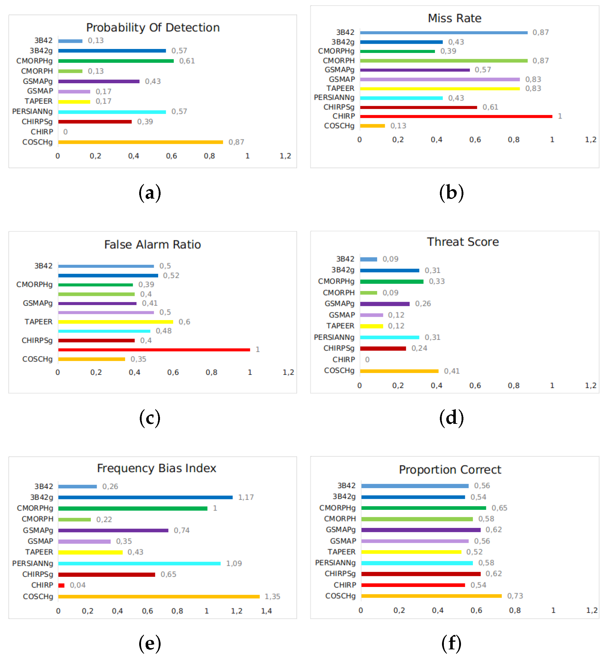
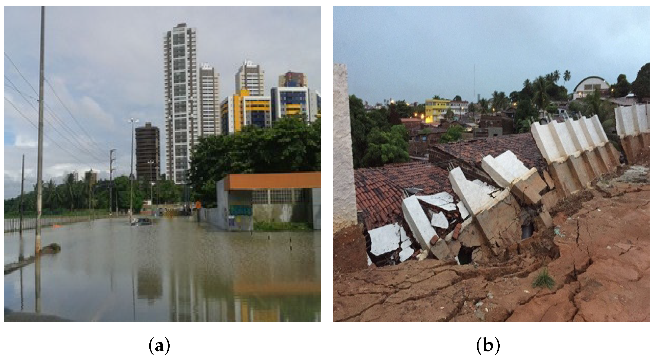
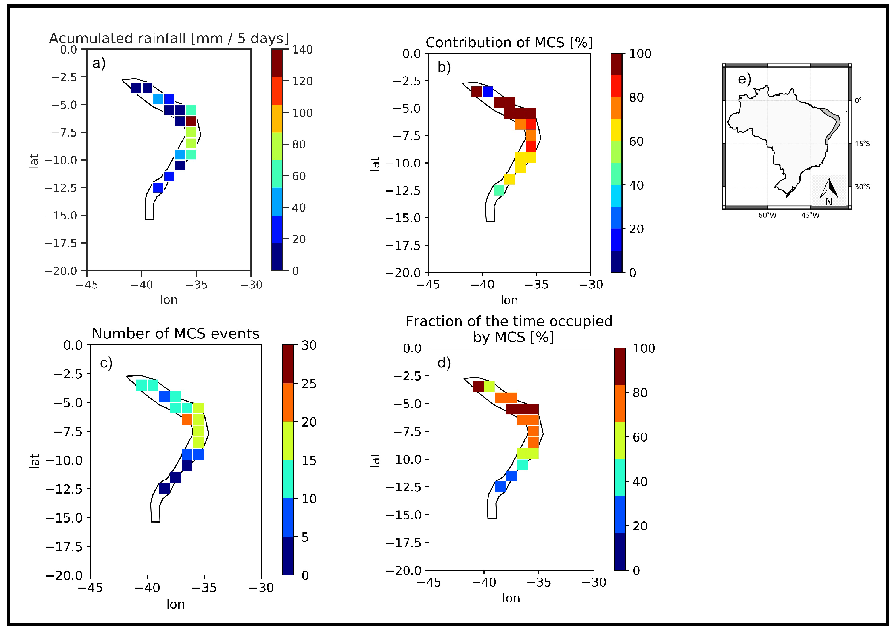
3.3. Case Study for Northeastern—R3
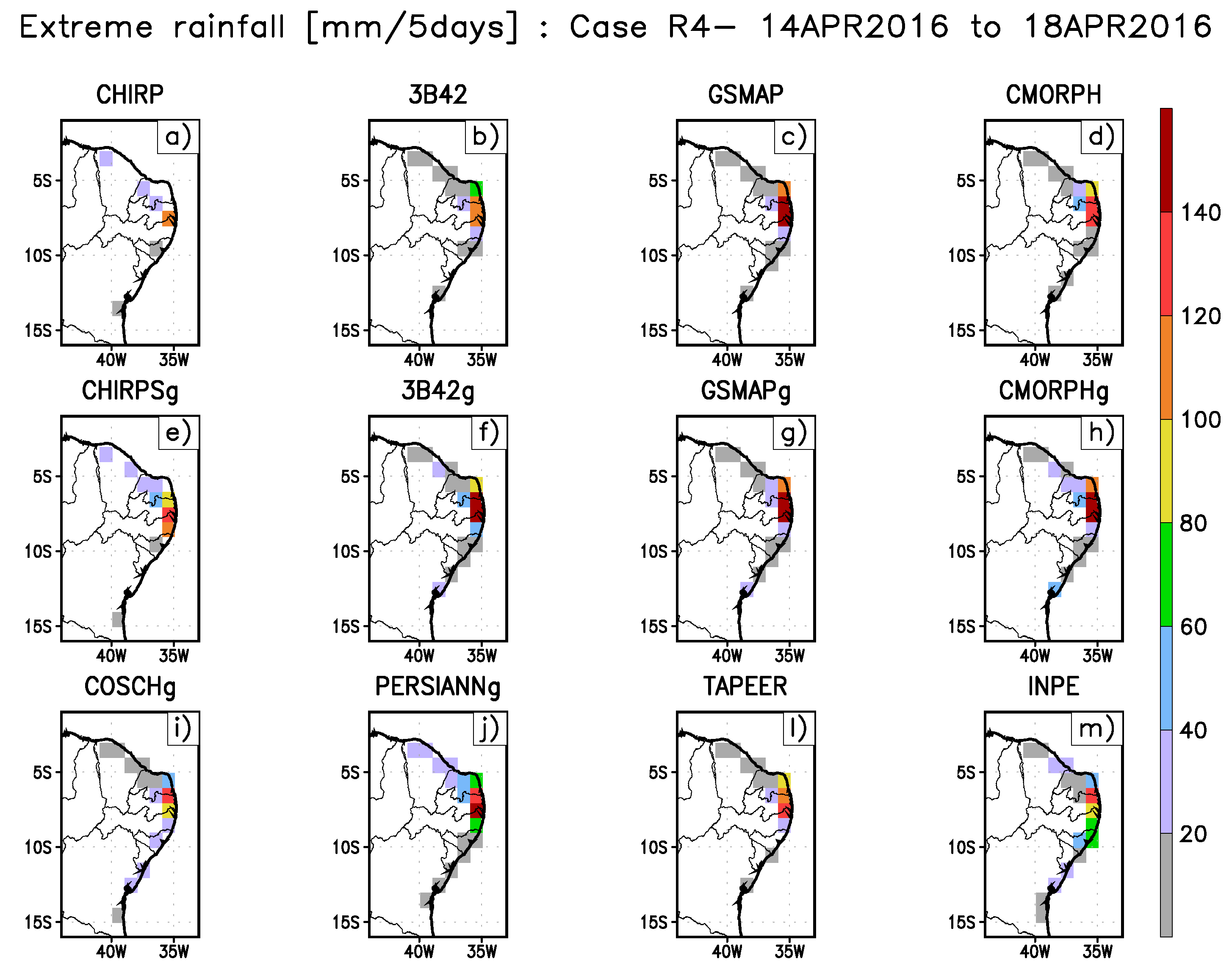
3.4. Case Study for Northeast Coast—R4
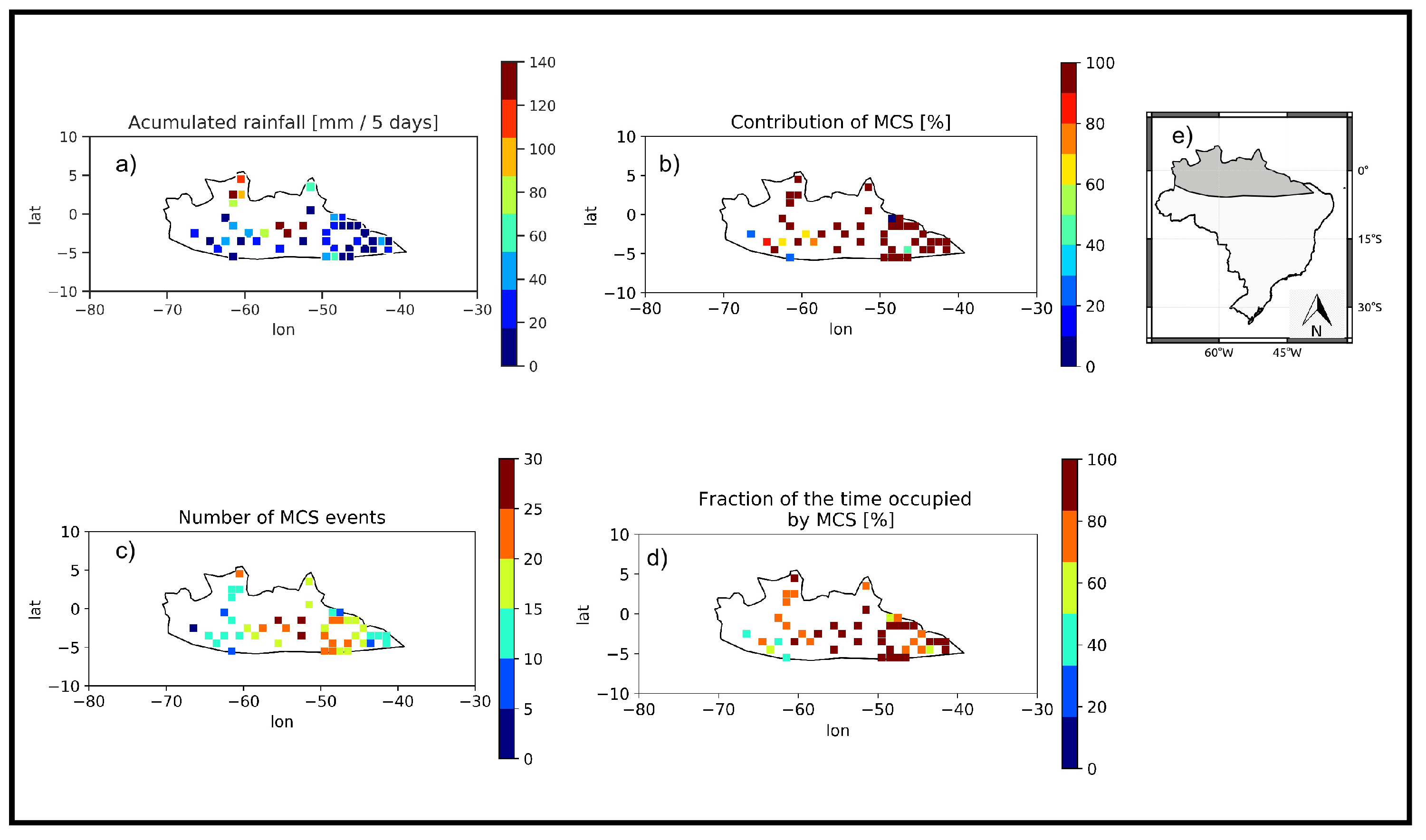
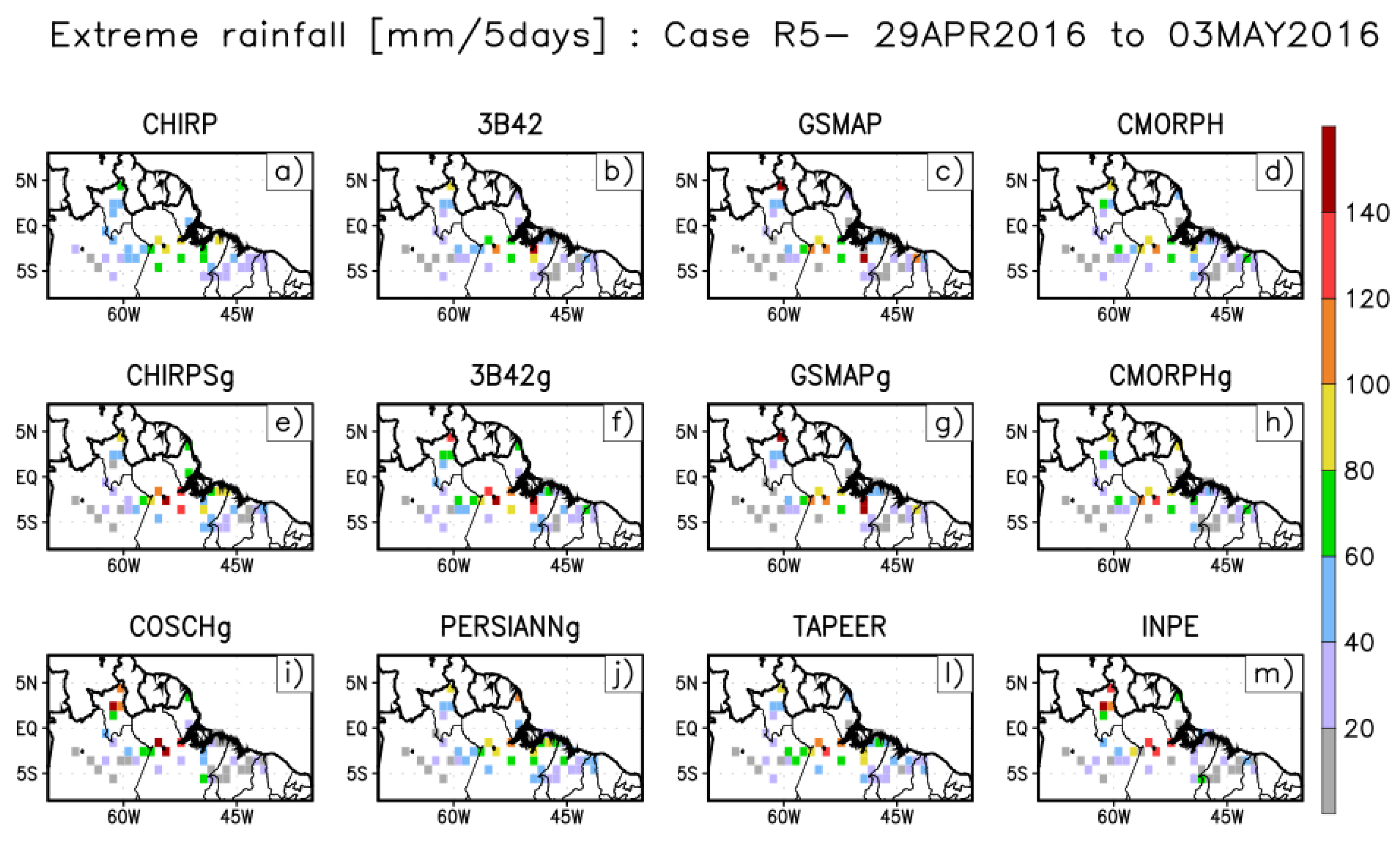
3.5. Case Study for North Brazil—R5
4. Conclusions
Author Contributions
Funding
Institutional Review Board Statement
Informed Consent Statement
Data Availability Statement
Acknowledgments
Conflicts of Interest
References
- Seneviratne, S.I.; Nicholls, N.; Easterling, D.; Goodess, C.M.; Kanae, S.; Kossin, J.; Luo, Y.; Marengo, J.; Mc Innes, K.; Rahimi, M.; et al. Changes in climate extremes and their impacts on the natural physical environment. Special report. Manag. Risks Extrem. Events Disasters Adv. Clim. Chang. Adapt. 2012, 109–230. [Google Scholar] [CrossRef] [Green Version]
- Centro Universitário de Estudos e Pesquisas sobre Desastres—CEPED; Universidade Federal de Santa Catarina. Atlas Brasileiro de Desastres Naturais: 1991 a 2012/Centro Universitário de Estudos e Pesquisas sobre Desastres. 2. ed. rev. ampl.–Florianópolis: CEPED UFSC, 2013.126 p. : il. color. ; 22 cm; CEPED: Florianópolis, Brazil, 2012; p. 94. Available online: https://www.ceped.ufsc.br/wp-content/uploads/2012/01/AMAZONAS_mioloWEB.pdf (accessed on 15 July 2022).
- Debortoli, N.S.; Camarinha, P.I.M.; Marengo, J.A.; Rodrigues, R.R. An index of Brazil’s vulnerability to expected increases in natural flash flooding and landslide disasters in the context of climate change. Nat. Hazards 2017, 86, 557–582. [Google Scholar] [CrossRef]
- Durkee, J.D.; Mote, T.L.; Shepherd, J.M. The contribution of mesoscale convective complexes to rainfall across subtropical South America. J. Clim. 2009, 22, 4590–4605. [Google Scholar] [CrossRef]
- Velasco, I.; Fritsch, J.M. Mesoscale convective complexes in the Americas. J. Geophys. Res. Atmos. 1987, 92, 9591–9613. [Google Scholar] [CrossRef]
- Grimm, A.M.; Barros, V.R.; Doyle, M.E. Climate variability in southern South America associated with El Niño and La Niña events. J. Clim. 2000, 13, 35–58. [Google Scholar] [CrossRef]
- Marengo, J.A.; Hastenrath, S. Case studies of extreme climatic events in the Amazon Basin. J. Clim. 1993, 6, 617–627. [Google Scholar] [CrossRef]
- Cohen, J.C.P.; Silva Dias, M.A.F.; Nobre, C.A. Environmental conditions associated with Amazonian squall lines: A case study. Mon. Weather Rev. 1995, 123, 3163–3174. [Google Scholar] [CrossRef]
- Yamazaki, Y.; Rao, V.B. Tropical cloudiness over the South Atlantic ocean. J. Meteorol. Soc. Jpn. 1977, 55, 205–207. [Google Scholar] [CrossRef] [Green Version]
- Gomes, H.B.; Ambrizzi, T.; Herdies, D.L.; Hodges, K.; Pontes da Silva, B.F. Easterly wave disturbances over Northeast Brazil: An observational analysis. Adv. Meteorol. 2015, 2015, 176238. [Google Scholar] [CrossRef] [Green Version]
- Xu, L.; Gao, X.; Sorooshian, S.; Arkin, P.A.; Imam, B. A microwave infrared threshold technique to improve the GOES precipitation index. J. Appl. Meteorol. 1999, 38, 569–579. [Google Scholar] [CrossRef]
- Turk, F.J.; Miller, S.D. Toward improved characterization of remotely sensed precipitation regimes with MODIS/AMSR-E blended data techniques. IEEE Trans. Geosci. Remote Sens. 2005, 43, 1059–1069. [Google Scholar] [CrossRef]
- Kida, S.; Shige, S.; Kubota, T.; Aonashi, K.; Okamoto, K. Improvement of rain/no-rain classification methods for microwave radiometer observations over the ocean using a 37 Ghz emission signature. J. Meteorol. Soc. Jpn. 2009, 87 A, 165–181. [Google Scholar] [CrossRef] [Green Version]
- Vila, D.A.; de Goncalves, L.G.G.; Toll, D.L.; Rozante, J.R. Statistical Evaluation of Combined Daily Gauge Observations and Rainfall Satellite Estimates over Continental South America. J. Hydrometeorol. 2009, 10, 533–543. [Google Scholar] [CrossRef]
- Shige, S.; Kida, S.; Ashiwake, H.; Kubota, T.; Aonashi, K. Improvement of TMI rain retrievals in mountainous areas. J. Appl. Meteorol. Climatol. 2013, 52, 242–254. [Google Scholar] [CrossRef] [Green Version]
- Kuligowski, R.J.; Li, Y.; Hao, Y.; Zhang, Y. Improvements to the GOES-R rainfall rate algorithm. J. Hydrometeorol. 2016, 17, 1693–1704. [Google Scholar] [CrossRef]
- Kidd, C.; Takayabu, Y.N.; Skofronick-Jackson, G.M.; Huffman, G.J.; Braun, S.A.; Kubota, T.; Turk, F.J. The Global Precipitation Measurement (GPM) mission. In Satellite Precipitation Measurements Vol. 1; Levizzani, V., Kidd, C., Kirschbaum, D.B., Kummerow, C.D., Nakamura, K., Turk, F.J., Eds.; Springer International Publishing: Berlin, Germany, 2020; Chapter 1; pp. 3–23. [Google Scholar] [CrossRef]
- Funk, C.; Peterson, P.; Landsfeld, M.; Davenport, F.; Becker, A.; Schneider, U.; Pedreros, D.; McNally, A.; Arsenault, K.; Harrison, L.; et al. Algorithm and Data Improvements for Version 2.1 of the Climate Hazards Center’s InfraRed Precipitation with Stations Dataset; Springer: Berlin, Germany, 2020; Volume 1, pp. 209–427. [Google Scholar]
- Kubota, T.; Aonashi, K.; Ushio, T.; Shige, S.; Takayabu, Y.N.; Kachi, M.; Arai, Y.; Tashima, T.; Masaki, T.; Kawamoto, N.; et al. Global Satellite Mapping of Precipitation (GSMaP) products in the GPM Era. In Satellite Precipitation Measurements Vol. 1; Levizzani, V., Kidd, C., Kirschbaum, D.B., Kummerow, C.D., Nakamura, K., Joseph Turk, F., Eds.; Springer International Publishing: Berlin, Germany, 2020; Volume 20, pp. 355–373. [Google Scholar] [CrossRef]
- Rozante, J.R.; Moreira, D.S.; de Goncalves, L.G.G.; Vila, D.A. Combining TRMM and surface observations of precipitation: Technique and validation over South America. Weather Forecast 2010, 25, 885–894. [Google Scholar] [CrossRef] [Green Version]
- Scofield, R.A.; Kuligowski, R.J. Status and outlook of operational satellite precipitation algorithms for extreme precipitation events. Weather Forecast 2003, 18, 1037–1051. [Google Scholar] [CrossRef]
- Funk, C.; Peterson, P.; Landsfeld, M.; Pedreros, D.; Verdin, J.; Shukla, S.; Husak, G.; Rowland, J.; Harrison, L.; Hoell, A.; et al. The climate hazards infrared precipitation with stations - a new environmental record for monitoring extremes. Sci. Data 2015, 2, 1–21. [Google Scholar] [CrossRef] [PubMed]
- Salio, P.; Hobouchian, M.P.; GARCÍA SKABAR, Y.; Vila, D. Evaluation of high-resolution satellite precipitation estimates over southern South America using a dense rain gauge network. Atmos. Res. 2015, 163, 146–161. [Google Scholar] [CrossRef]
- Amitai, E.; Petersen, W.; Llort, X.; Vasiloff, S. Multiplatform comparisons of rain intensity for extreme precipitation events. IEEE Trans. Geosci. Remote Sens. 2012, 50, 675–686. [Google Scholar] [CrossRef]
- Masunaga, H.; Schröder, M.; Furuzawa, F.A.; Kummerow, C.; Rustemeier, E.; Schneider, U. Inter-product biases in global precipitation extremes. Environ. Res. Lett. 2019, 14, 125016. [Google Scholar] [CrossRef]
- Liu, J.; Xia, J.; She, D.; Li, L.; Wang, Q.; Zou, L. Evaluation of six satellite-based precipitation products and their ability for capturing characteristics of extreme precipitation events over a climate transition area in China. Remote Sens. 2019, 11, 1477. [Google Scholar] [CrossRef] [Green Version]
- Palharini, R.S.A.; Vila, D.A.; Rodrigues, D.T.; Quispe, D.P.; Palharini, R.C.; Siqueira, R.A.D.; Afonso, J.M.D.S. Assessment of the extreme precipitation by satellite estimates over South America. Remote Sens. 2020, 12, 2085. [Google Scholar] [CrossRef]
- Reboita, M.S.; Gan, M.A.; da Rocha, R.P.; Ambrizzi, T. Regimes de precipitação na América do Sul: Uma revisão bibliográfica. Rev. Bras. De Meteorol. 2010, 25, 185–204. [Google Scholar] [CrossRef]
- Rozante, J.R.; Vila, D.A.; Chiquetto, J.B.; Fernandes, A.; Alvim, D.S. Evaluation of TRMM/GPM blended daily products over Brazil. Remote Sens. 2018, 10, 882. [Google Scholar] [CrossRef] [Green Version]
- Diniz, F.d.A.; Ramos, A.M.; Rebello, E.R.G. Brazilian climate normals for 1981-2010. Pesqui. Agropecu. Bras. 2018, 53, 131–143. [Google Scholar] [CrossRef]
- Lyra, M.J.; Fedorova, N.; Levit, V. Mesoscale convective complexes over northeastern Brazil. J. South Am. Earth Sci. 2022, 118, 103911. [Google Scholar] [CrossRef]
- Silva Dias, M.A.F.d. Sistemas de mesoescala e previsão de tempo a curto prazo. Rev. Bras. De Meteorol. 1987, 2, 133–150. [Google Scholar]
- Grimm, A.M. The El Niño Impact on the Summer Monsoon in Brazil: Regional Processes versus Remote Influences. J. Clim. 2003, 2, 263–280. [Google Scholar] [CrossRef]
- Schossler, V.; Simões, J.C.; Aquino, F.E.; Viana, D.R. Precipitation anomalies in the Brazilian southern coast related to the SAM and ENSO climate variability modes. RBRH 2018, 23, 3761–3780. [Google Scholar] [CrossRef] [Green Version]
- Jimenez, J.C.; Marengo, J.A.; Alves, L.M.; Sulca, J.C.; Takahashi, K.; Ferrett, S.; Collins, M. The role of ENSO flavours and TNA on recent droughts over Amazonforests and the Northeast Brazil region. Int. J. Climatol. 2021, 41, 3761–3780. [Google Scholar] [CrossRef]
- Vera, C.; Baez, J.; Douglas, M.; Emmanuel, C.B.; Marengo, J.; Meitin, J.; Nicolini, M.; Nogues-Paegle, J.; Paegle, J.; Penalba, O.; et al. The South American low-level jet experiment. Bull. Am. Meteorol. Soc. 2006, 87, 63–77. [Google Scholar] [CrossRef]
- Lenters, J.D.; Cook, K.H. Simulation and diagnosis of the regional summertime precipitation climatology of South America. J. Clim. 1995, 8, 2988–3005. [Google Scholar] [CrossRef]
- Rosa, E.B.; Pezzi, L.P.; de Quadro, M.F.L.; Brunsell, N. Automated detection algorithm for SACZ, oceanic SACZ, and their climatological features. Front. Environ. Sci. 2020, 8, 18. [Google Scholar] [CrossRef]
- Zhou, J.; Lau, K.M. Does a monsoon climate exist over South America? J. Clim. 1998, 11, 1020–1040. [Google Scholar] [CrossRef]
- Rao, V.B.; Franchito, S.H.; Santo, C.M.; Gan, M.A. An update on the rainfall characteristics of Brazil: Seasonal variations and trends in 1979–2011. Int. J. Climatol. 2016, 36, 291–302. [Google Scholar] [CrossRef]
- Kousky, V.E.; Gan, M.A. Upper tropospheric cyclonic vortices in the tropical South Atlantic. Tellus 1981, 33, 538–551. [Google Scholar] [CrossRef] [Green Version]
- Palharini, R.S.A.; Vila, D.A. Climatological behavior of precipitating clouds in the northeast region of Brazil. Adv. Meteorol. 2017, 2017, 17–21. [Google Scholar] [CrossRef] [Green Version]
- Kousky, V.E.; Chug, P.S. Fluctuations in annual rainfall for northeast Brazil. J. Meteorol. Soc. Jpn. 1978, 56, 457–465. [Google Scholar] [CrossRef]
- Roca, R.; Alexander, L.V.; Potter, G.; Bador, M.; Jucá, R.; Contractor, S.; Bosilovich, M.G.; Cloché, S. FROGS: A daily 1° × 1° gridded precipitation database of rain gauge, satellite and reanalysis products. Earth Syst. Sci. Data 2019, 11, 1017–1035. [Google Scholar] [CrossRef] [Green Version]
- Fiolleau, T.; Roca, R. An algorithm for the detection and tracking of tropical mesoscale convective systems using infrared images from geostationary satellite. IEEE Trans. Geosci. Remote Sens. 2013, 51, 4302–4315. [Google Scholar] [CrossRef]
- Roca, R.; Ramanathan, V. Scale dependence of monsoonal convective systems over the Indian Ocean. J. Clim. 2000, 13, 1286–1298. [Google Scholar] [CrossRef]
- Robert, A. Cloud clusters and large-scale vertical motions in the tropics. J. Meteorol. Soc. Jpn. 1982, 60, 396–410. [Google Scholar]
- Wilks, D. Statistical Methods in the Atmopspheric Sciencies, 3rd ed.; Elsevier: Cambridge, MA, USA, 2011. [Google Scholar]
- Olmo, M.; Bettolli, M. Extreme daily precipitation in southern South America: Statistical characterization and circulation types using observational datasets and regional climate models. Clim. Dyn. 2021, 57, 895–916. [Google Scholar] [CrossRef]
- Salio, P.; Nicolini, M.; Zipser, E.J. Mesoscale Convective Systems over Southeastern South America and Their Relationship with the South American Low-Level Jet. Mon. Weather Rev. 2007, 135, 1290–1309. [Google Scholar] [CrossRef] [Green Version]
- Rasmussen, K.L.; Chaplin, M.M.; Zuluaga, M.D.; Houze, R.A. Contribution of extreme convective storms to rainfall in South America. J. Hydrometeorol. 2016, 17, 353–367. [Google Scholar] [CrossRef]
- Silva, J.; Reboita, M.; Escobar, G. Caracterização da zona de convergência do Atlântico Sul em campos atmosféricos recentes. Rev. Bras. Climatol. 2019, 25, 355–377. [Google Scholar] [CrossRef] [Green Version]
- Rodrigues, D.T.; Gonçalves, W.A.; Spyrides, M.H.C.; Santos e Silva, C.M. Spatial and temporal assessment of the extreme and daily precipitation of the Tropical Rainfall Measuring Mission satellite in Northeast Brazil. Int. J. Remote Sens. 2019, 41, 549–572. [Google Scholar] [CrossRef]
- Rodrigues, D.T.; Gonçalves, W.A.; Spyrides, M.H.; Santos e Silva, C.M.; de Souza, D.O. Spatial distribution of the level of return of extreme precipitation events in Northeast Brazil. Int. J. Climatol. 2020, 40, 5098–5113. [Google Scholar] [CrossRef]
- Escobar, G.; Matoso, V. Zona de CONVERGÊNCIA do Atlântico Sul (ZCAS): Definição prática segundo uma visão operacional. In Anais do XX Congresso Brasileiro de Meteorologia, 27 a 30 de Novembro 2018, Maceio, AL [Recurso Eletrônico]/Coordenado por Heliofábio Barros Gomes; UFAL: Maceio, Brazil, 2018. [Google Scholar]
- Rodrigues, D.T.; Santos e Silva, C.M.; dos Reis, J.S.; Palharini, R.S.A.; Cabral Júnior, J.B.; da Silva, H.J.F.; Mutti, P.R.; Bezerra, B.G.; Gonçalves, W.A. Evaluation of the Integrated Multi-SatellitE Retrievals for the Global Precipitation Measurement (IMERG) Product in the São Francisco Basin (Brazil). Water 2021, 13, 2714. [Google Scholar] [CrossRef]
- Rodrigues, D.T.; Gonçalves, W.A.; Spyrides, M.H.C.; Andrade, L.D.M.B.; de Souza, D.O.; de Araujo, P.A.A.; Santos e Silva, C.M.S. Probability of occurrence of extreme precipitation events and natural disasters in the city of Natal, Brazil. Urban Clim. 2021, 35, 100753. [Google Scholar] [CrossRef]
- Morales, F.E.C.; Rodrigues, D.T. Spatiotemporal nonhomogeneous poisson model with a seasonal component applied to the analysis of extreme rainfall. J. Appl. Stat. 2022, 1, 1–19. [Google Scholar] [CrossRef]
- Palharini, R.S.A.; Vila, D.A.; Rodrigues, D.T.; Palharini, R.C.; Mattos, E.V.; Pedra, G.U. Assessment of extreme rainfall estimates from satellite-based: Regional analysis. Remote Sens. Appl. Soc. Environ. 2021, 23, 100603. [Google Scholar] [CrossRef]
- Vila, D.A.; Oliveira, R.A.J.; Biscaro, T.S.; Mattos, E.V.; Cecchini, M.A. Chapter 18 - Cloud processes of the main precipitating systems over continental tropical regions. In Precipitation Science; Michaelides, S., Ed.; Elsevier: Amsterdam, The Netherlands, 2022; pp. 561–614. [Google Scholar] [CrossRef]
- Machado, L.A.T.; Calheiros, A.J.; Biscaro, T.; Giangrande, S.; Silva Dias, M.A.F.; Cecchini, M.; Albrecht, R.; Andreae, M.; Araujo, W.; Artaxo, P.; et al. Overview: Precipitation characteristics and sensitivities to environmental conditions during GoAmazon2014/5 and ACRIDICON-CHUVA. Atmos. Res. 2018, 18, 6461–64820. [Google Scholar] [CrossRef] [Green Version]
- Cecchini, M.; Machado, L.; Artaxo, P. Droplet size distributions as a function of rainy system type and cloud condensation nuclei concentrations. Atmos. Res. 2014, 143, 301–312. [Google Scholar] [CrossRef]
- Calheiros, A.J.; Machado, L.A.T. Cloud and rain liquid water statistics in the CHUVA campaign. Atmos. Res. 2014, 144, 126–140. [Google Scholar] [CrossRef]
- Petković, V.; Kummerow, C.D.; Randel, D.L.; Pierce, J.R.; Kodros, J.K. Improving the Quality of Heavy Precipitation Estimates from Satellite Passive Microwave Rainfall Retrievals. J. Hydrometeorol. 2017, 19, 69–85. [Google Scholar] [CrossRef]
- Petković, V.; Kummerow, C.D. Understanding the sources of satellite passive microwave rainfall retrieval systematic errors over land. J. Appl. Meteorol. Climatol. 2017, 56, 597–614. [Google Scholar] [CrossRef]
- Kimani, M.W.; Hoedjes, J.C.; Su, Z. An assessment of satellite-derived rainfall products relative to ground observations over East Africa. Remote Sens. 2017, 9, 430. [Google Scholar] [CrossRef]
- Ye, X.; Guo, Y.; Wang, Z.; Liang, L.; Tian, J. Extensive Evaluation of Four Satellite Precipitation Products and Their Hydrologic Applications over the Yarlung Zangbo River. Remote Sens. 2022, 14, 3350. [Google Scholar] [CrossRef]


| Satellite Product Version | Short Name | Use Rain Gauges | Use IR Sensor | Use MW Sensor |
|---|---|---|---|---|
| CHIRP v2.0 | CHIRP | No | Yes | No |
| CHIRPS v2.0 | CHIRPSg | Yes | Yes | No |
| PERSIANN CDR v1 r1 | PERSIANNg | Yes | Yes | No |
| 3B42 RT v7.0 uncalibrated | 3B42 | No | Yes | Yes |
| 3B42 RT v7.0 | 3B42g | Yes | Yes | Yes |
| GSMAP-NRT-no gauges v6.0 | GSMAP | No | Yes | Yes |
| GSMAP-NRT-gauges v6.0 | GSMAPg | Yes | Yes | Yes |
| CMORPH V1.0, RAW | CMORPH | No | Yes | Yes |
| CMORPH V1.0, CRT | CMORPHg | Yes | Yes | Yes |
| TAPEER v1.5 | TAPEER | No | Yes | Yes |
| COSCH | COSCHg | Yes | Yes | Yes |
| Region | Date | Rainfall | Affected People |
|---|---|---|---|
| R1 | 24 June 2014 to 28 June 2014 | >300 mm/5 days | 1600 |
| R2 | 01 January 2012 to 05 January 2012 | >140 mm/5 days | 200,000 |
| R3 | 20 January 2016 to 24 January 2016 | >200 mm/5 days | No information in civil defence report |
| R4 | 14 April 2016 to 18 April 2016 | >200 mm/5 days | 2268 |
| R5 | 29 April 2016 to 03 May 2016 | >140 mm/5 days | 15,265 |
| Gauge ≥ Threshold | Gauge < Threshold | |
|---|---|---|
| Satellite ≥ Threshold | Hits (A) | False Alarms (B) |
| Satellite < Threshold | Misses (C) | Correct Negatives (D) |
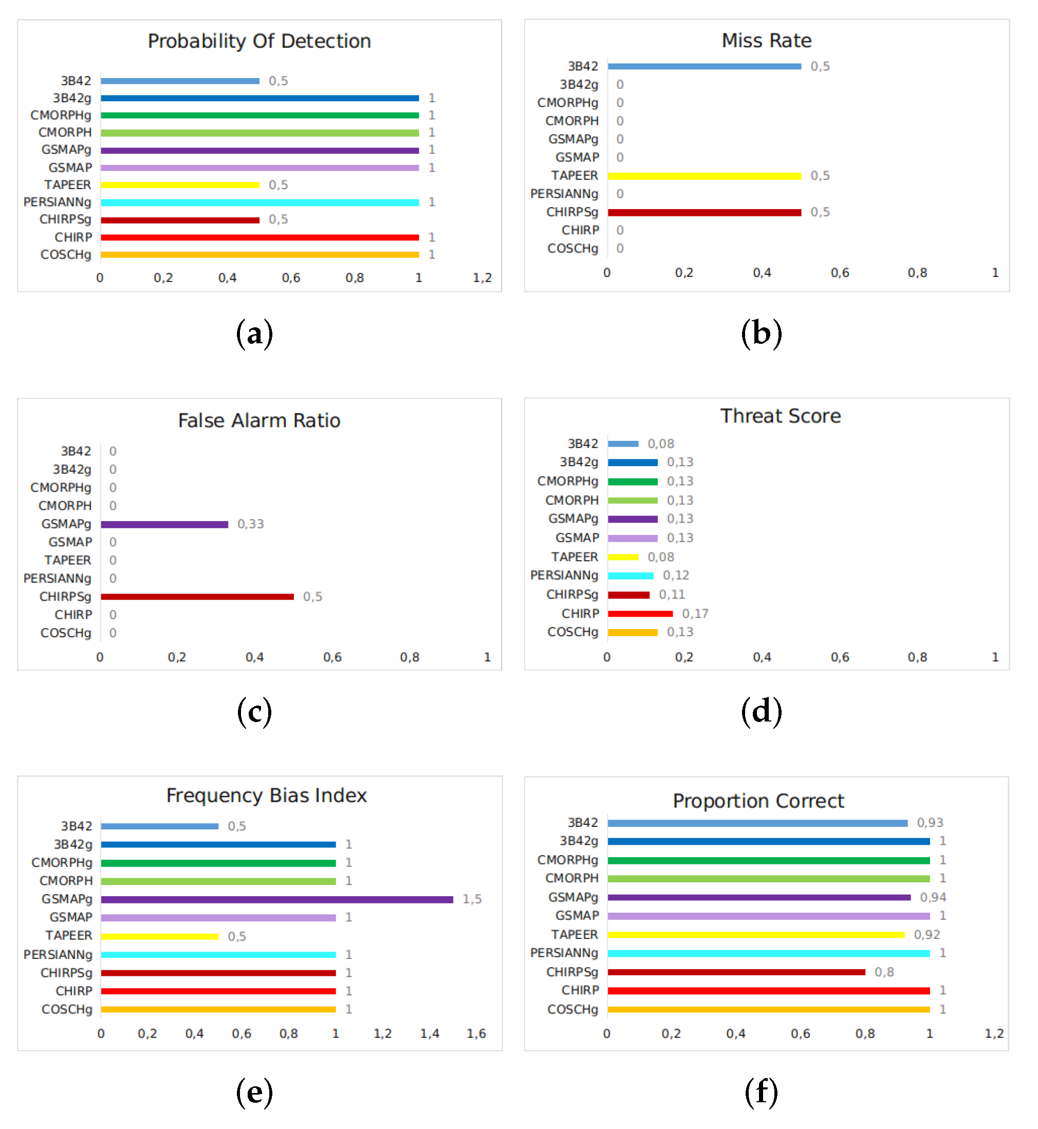
| Statistical Measure | Equation | Range | Perfect Score |
|---|---|---|---|
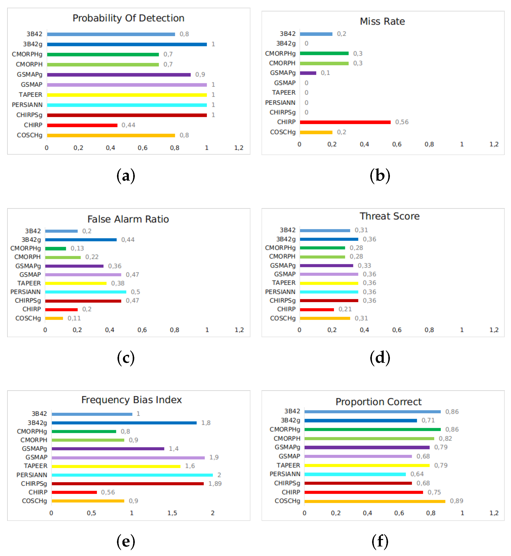
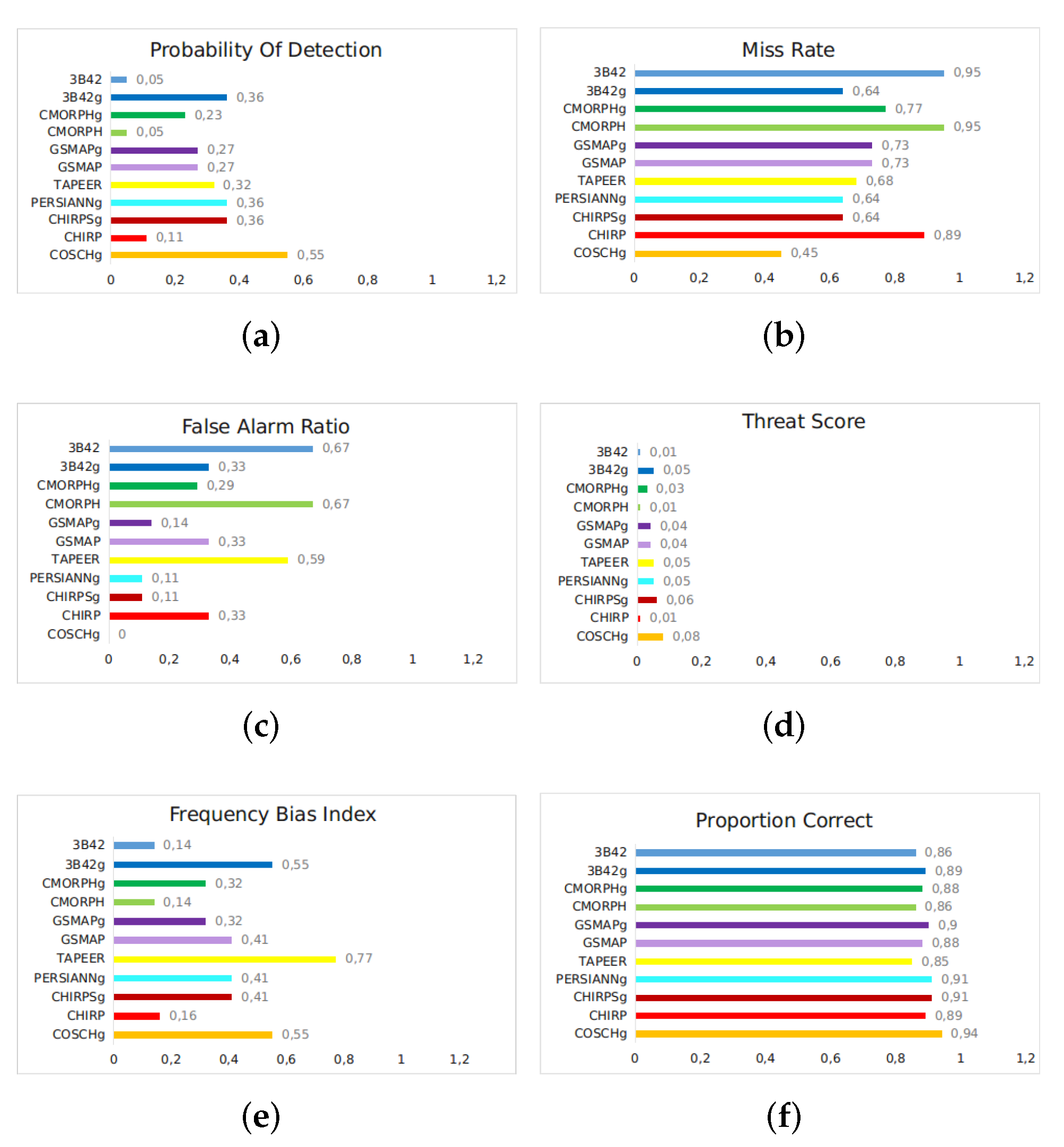
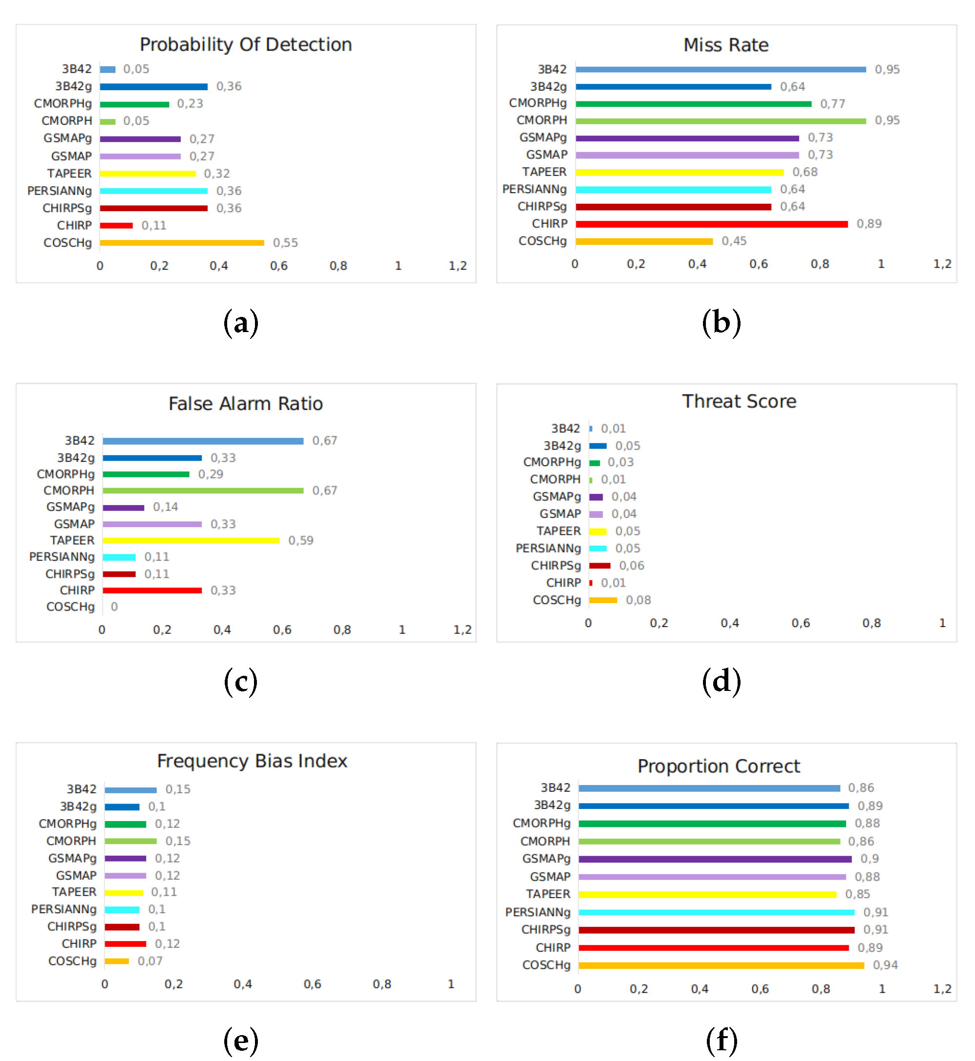
| POD | A/(A + C) | 0 to 1 | 1 |
| MR | C/(A + C) | 0 to 1 | 0 |
| FAR | B/(A + B) | 0 to 1 | 0 |
| TS | A/(A + B + C) | 0 to 1 | 1 |
| FBI | (A + B)/(A + C) | 0 to ∞ | 1 |
| PC | (A + D)/(A + B + C + D) | 0 to 1 | 1 |
Publisher’s Note: MDPI stays neutral with regard to jurisdictional claims in published maps and institutional affiliations. |
© 2022 by the authors. Licensee MDPI, Basel, Switzerland. This article is an open access article distributed under the terms and conditions of the Creative Commons Attribution (CC BY) license (https://creativecommons.org/licenses/by/4.0/).
Share and Cite
Palharini, R.; Vila, D.; Rodrigues, D.; Palharini, R.; Mattos, E.; Undurraga, E. Analysis of Extreme Rainfall and Natural Disasters Events Using Satellite Precipitation Products in Different Regions of Brazil. Atmosphere 2022, 13, 1680. https://doi.org/10.3390/atmos13101680
Palharini R, Vila D, Rodrigues D, Palharini R, Mattos E, Undurraga E. Analysis of Extreme Rainfall and Natural Disasters Events Using Satellite Precipitation Products in Different Regions of Brazil. Atmosphere. 2022; 13(10):1680. https://doi.org/10.3390/atmos13101680
Chicago/Turabian StylePalharini, Rayana, Daniel Vila, Daniele Rodrigues, Rodrigo Palharini, Enrique Mattos, and Eduardo Undurraga. 2022. "Analysis of Extreme Rainfall and Natural Disasters Events Using Satellite Precipitation Products in Different Regions of Brazil" Atmosphere 13, no. 10: 1680. https://doi.org/10.3390/atmos13101680