
How Photochemically Consumed Volatile Organic Compounds Affect Ozone Formation: A Case Study in Chengdu, China


1
Chengdu Academy of Environmental Sciences, Chengdu 610072, China
2
College of Architecture and Environment, Sichuan University, Chengdu 610065, China
*
Author to whom correspondence should be addressed.
Atmosphere 2022, 13(10), 1534; https://doi.org/10.3390/atmos13101534
Submission received: 31 July 2022
/
Revised: 12 September 2022
/
Accepted: 12 September 2022
/
Published: 20 September 2022
(This article belongs to the Special Issue Insights into Volatile Organic Compounds in the Atmosphere: Component Characteristics, Source Apportionment and Environmental Implications)
Abstract
:Surface ozone (O3) pollution has not improved significantly in recent years. It is still the primary air pollution problem in many megacities in China during summertime. In high temperature and intense radiation weather, volatile organic compounds (VOCs) are easily oxidized and degraded to induce O3 pollution. In order to understand the impact of difference between photochemical initial concentration (PIC) of VOCs and the actual measured concentration on O3 formation, a campaign was carried out during O3 pollution in Chengdu (25 July–5 August 2021). During this O3 pollution episode, the maximum value of O3 concentration reached 335.0 μg/m3, and the precursor concentrations increased significantly. The mean values of VOCmeasured and VOCPICs were 19.7 ppbv and 30.7 ppbv, corresponding to O3 formation potential (OFP) of 175.3 μg/m3 and 478.8 μg/m3, respectively, indicating that the consumption of VOCs content could not be ignored. Alkenes accounted for 77.2% of VOCs consumption. Alkenes and aromatics contributed 63.0% and 29.2% to OFP values which derived from PIC of each VOC species. The relative incremental reactivity analysis based on PICs showed that the O3 formation was controlled by the cooperation of nitrogen oxides (NOx) and VOCs, and the effect of NOx emission reduction was better.
1. Introduction
In recent years, air pollution has become the primary pollution problem in China. In summer, when the sun radiation is more intense, photochemical smog pollution is more likely to occur. Ozone (O3) is a symbolic product of photochemical smog. Due to its high oxidizing properties, O3 in the troposphere participates in heterogeneous chemical processes in the atmosphere, formation of secondary aerosols and other processes, and will directly affect the health of human respiratory system and the growth of crops [1,2]. Nitrogen oxides (NOx) and volatile organic compounds (VOCs) are precursors of O3. Furthermore, high temperature and intense radiation also affect the formation of O3. Coupled with the influence of regional transportation, it is more difficult to judge the cause of ozone pollution. Therefore, in addition to the temporal and spatial distribution characteristics of O3 concentration, it has become a research hotspot in this field to explore the control and emission reduction of O3 pollution by strengthening the distribution of precursor sources and their influence on the formation of O3.
The ozone formation potential (OFP) is widely used to estimate the relative contribution of VOCs to O3 formation. In the vast majority of studies, the measured value of VOC concentrations was used directly to calculate OFP [3,4,5,6,7]. Due to the high activity of VOCs, the photochemical aging rate is faster after being discharged into the atmosphere, resulting in a certain difference between the concentration and composition of VOCs monitored and the actual emission [8]. When considering photochemical consumption, the contribution of different VOC species to O3 generation varies greatly, especially for alkenes [9,10]. When studying O3 pollution, the concept of photochemical initial concentration (PIC) is introduced, which can be used to restore the content of VOCs in the real atmospheric environment. PIC was more consistent in the verification of the localized VOCs source spectrum emission characteristics and the source inventory, which can improve the reliability of the simulation results of the source analysis model [11,12]. Further calculation of OFP using the PIC of VOCs is very friendly to identify key active species that affect the formation of local O3, providing insight into the mechanism of O3 formation and evolution [10,13].
Chengdu, located in the western edge of the Sichuan Basin in China, is one of the typical megacities in this region. The climate and environment of the Sichuan Basin are self-contained. Due to the depression of the terrain, high humidity and calm winds are very common [14]. The special climate and high concentration of precursors’ emissions aggravate the O3 pollution in Chengdu, especially in summer [7,15,16,17]. O3 pollution in Chengdu has a strong seasonality (the seasons mentioned in this study are relative to the Northern hemisphere). The current researches focused on spring, summer, and autumn [18,19,20,21,22]. In spring, O3 pollution is mostly combined with PM2.5 to form double high pollution. The studies on the sensitivity of O3 found that in the spring and autumn, O3 generation at urban areas was usually determined by VOCs, and the emission of anthropogenic VOCs was the key factor for the formation of O3 pollution in these areas, while some suburbs were coordinated control regimes, which were affected by the combined effects of VOCs and NOx [21,23,24]. At present, the effect of photochemical aging has not been included in the VOC concentrations study in Chengdu, and the contribution of photochemically consumed VOCs to O3 formation is still unclear. Therefore, it is necessary to study it.
We selected an O3 pollution episode for research at the urban area in Chengdu in summer 2021, focusing on the characteristics of O3 and its precursors before, during, and after the pollution. The initial VOCs emission concentration was estimated by using the photochemical aging parameterization equation, which was used to judge the key VOC species in the O3 formation and sensitivity analysis. The purpose was to explore the effect of VOC consumption on the formation and control of O3. The results of this work can provide optimization ideas for the control strategy of O3 pollution in this area.
2. Methods
2.1. Monitoring Site and Instruments
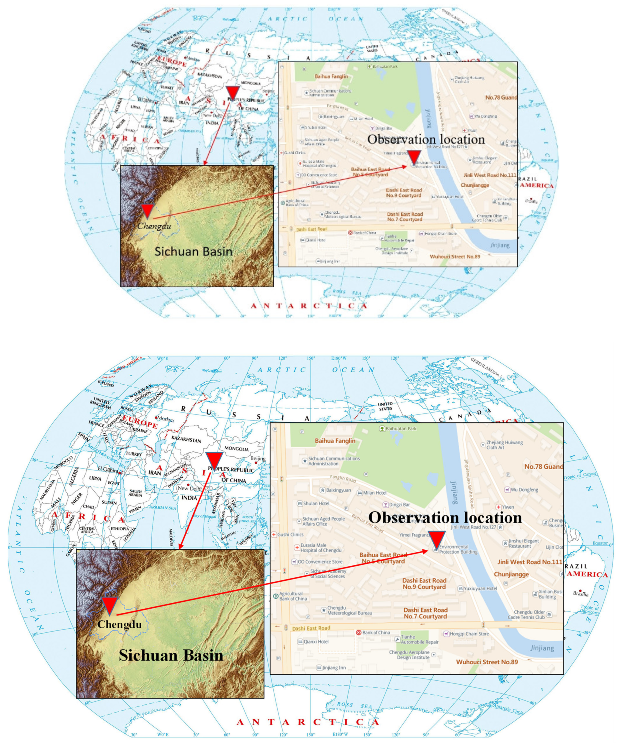
The monitoring site is located on the roof of the Chengdu Academy of Environmental Sciences (30°56′ E, 104°05′ N), Qingyang District, and the sampling site is about 25 m above the ground. Located within the First Ring Road of Chengdu, the site is an excellent location for a comprehensive observation of the mixed environment of transportation, commercial and residential infrastructure in the central city. The specific position is shown as the red inverted triangle in Figure 1.
VOC species were analyzed by an automated online system using a gas chromatograph (GC955-611/811, Synspec, Groningen, The Netherlands) with a flame ionization detector (FID, measuring low carbon hydrocarbons, C2–C5) and a dual photoionization detector (PID, measuring high carbon hydrocarbons, C6–C12). Hourly concentrations of 56 non-methane hydrocarbons (NMHC) were measured. Previous works, including the operation processes, quality assurance/quality control procedures, detection limits, and precision for the determination of VOCs, provided a detailed description of this instrument [19,25]. In this study, 47 VOC species were finally obtained, including alkanes (we define the number of VOC species as n, n = 25), alkenes (n = 9), and aromatics (n = 13).
The hourly concentrations of nitric oxide (NO), nitrogen dioxide (NO2), NOx, carbon monoxide (CO), O3, and sulfur dioxide (SO2) were continuously measured by i-series instruments (42i, 42i, 42i, 48i, 49i and 43i, respectively) manufactured by Thermo Fisher Corporation (USA). Continuous measurements of wind direction (WD), wind speed (WS), temperature (T), relative humidity (RH), pressure (P), and precipitation (PRE) were performed using a micro weather station instrument (WS600-UMB, Lufft, Germany). In addition, solar optical data (e.g., ultraviolet intensity, photolysis rate constant) and aerosol lidar data were also acquired.
2.2. Data Analysis
2.2.1. Contribution to O3 Formation
VOCs can promote O3 generation, and different VOC species have significant differences in O3 formation potential (OFP). In order to determine the contribution of VOCs to O3 generation and identify the main VOC active species, the maximum incremental reactivity (MIR) method was used in this study to calculate the OFP of 47 VOCs with MIR coefficients. The calculation formula is shown in Equation (1):
OFPi = [VOCi] × MIRi
In the formula, i is a VOC compound; OFPi is the O3 formation potential, μg/m3; [VOCi] is the VOC concentration, μg/m3; MIR is the maximum reactivity increment, g·O3/g·VOCs, the MIR values of each VOC species are all from previous works [26,27]. The MIRs used in this study are summarized in Table S1 of Supplementary Materials.
2.2.2. Photochemical Initial Concentration (PIC)
The photochemical aging parameterization method can be used to calculate the photochemical reaction time. It is usually calculated by the ratio of two VOC species with strong correlation (similar sources) and large difference in OH reaction rates [28]. Pollutants released into the atmosphere will immediately mix with the aging air mass, which causes uncertainty in the determination of the photochemical aging time, but this method is still an effective measure for atmospheric photochemical treatment [29]. The OH exposure ([OH]Δt, [OH]: OH radical concentration, Δt: photochemical reaction time) can be used as a whole to calculate the initial emission concentration. Previous studies have shown that m,p-xylene and ethylbenzene are very suitable for the calculation of PIC in urban areas [10,11,30,31]. Figure S1 shows a high correlation between m,p-xylene and ethylbenzene (r = 0.97, p < 0.01). [OH]Δt can be calculated from Equation (2):
[OH]Δt = (ln[X]/[E]|t=0 − ln[X]/[E]|t=t)/(kX − kE)
X represents m,p-xylene, E represents ethylbenzene. kX and kE are the reaction rate constants of m,p-xylene and ethylbenzene, which are 19.85 × 10⁻¹² cm3/molecule∙s and 7.51 × 10⁻¹² cm3/molecule∙s, respectively. The diurnal variation of m,p-xylene/ethylbenzene ratio over the entire period is shown in Figure S1, and the nighttime ratio was relatively stable and remained at a high value. In this study, the method for determining the initial concentration ratio of m,p-xylene/ethylbenzene ([X]/[E]|t=0) referred to the study of Yuan et al. [32], and the calculation result in [X]/[E]|t=0 was 3.27 ppbv/ppbv. The initial concentration of VOC species can be described by the following equation [31]:
where kVOCi is the reaction rate constant of [VOCi], cm3/molecule s, and the value of this constant refers to previous research [33].
dVOCi/dt = kVOCi × [VOCi] × [OH]
[VOCi]initial, t=0 = [VOCi]measured, t=t × exp(−kVOCi × [OH]Δt)
2.3. Observation-Based Model (OBM)
The chemical mechanism is the core part of the observation-based photochemical box model (OBM). In this study, a detailed chemical mechanism model, namely, Master Chemical Mechanism (MCM), was selected for simulation. MCM was proposed by Jenkin et al. to describe the detailed chemical processes of single VOC species in the atmosphere in 1997 [34]. It has now been developed to the MCM v3.3.1 version, which contains more than 140 primary VOC species and approximately 17,000 reactions [35,36]. The input module introduced an hourly changing sequence of 37 VOC species, 4 trace gases (NO, NO2, CO, and SO2), meteorological parameters (T, RH, P), and NO2 photolysis rate constant (JNO2) as constraint parameters in the model. The start time of OBM-MCM model simulation was set as 7:00 Chinese National Standard Time (CNST, UTC + 8), and the output results were in hourly resolution.
Based on OBM simulation, the relative incremental reactivity (RIR) of each precursor can be calculated, which can effectively quantify which type of precursor is the dominant substance for O3 generation [11,37,38]. The following Equation (5) can be used to derive the RIR value:
where x represents an O3 precursor; O3 represents the simulated O3 concentration in the base case; C(x) refers to the integrated source function (e.g., emission, transport) that affects the concentration of x species at the monitoring site. ΔO3(x)/O3 and ΔC(x)/C(x) represent the relative changes of O3 simulated concentration and x species concentration, respectively. In this study, we selected a 15% reduction in precursor emissions for RIR analysis.
RIR(x) = (ΔO3(x)/O3)/(ΔC(x)/C(x))
3. Results and Discussion
3.1. General Statistics
3.1.1. Data Overview
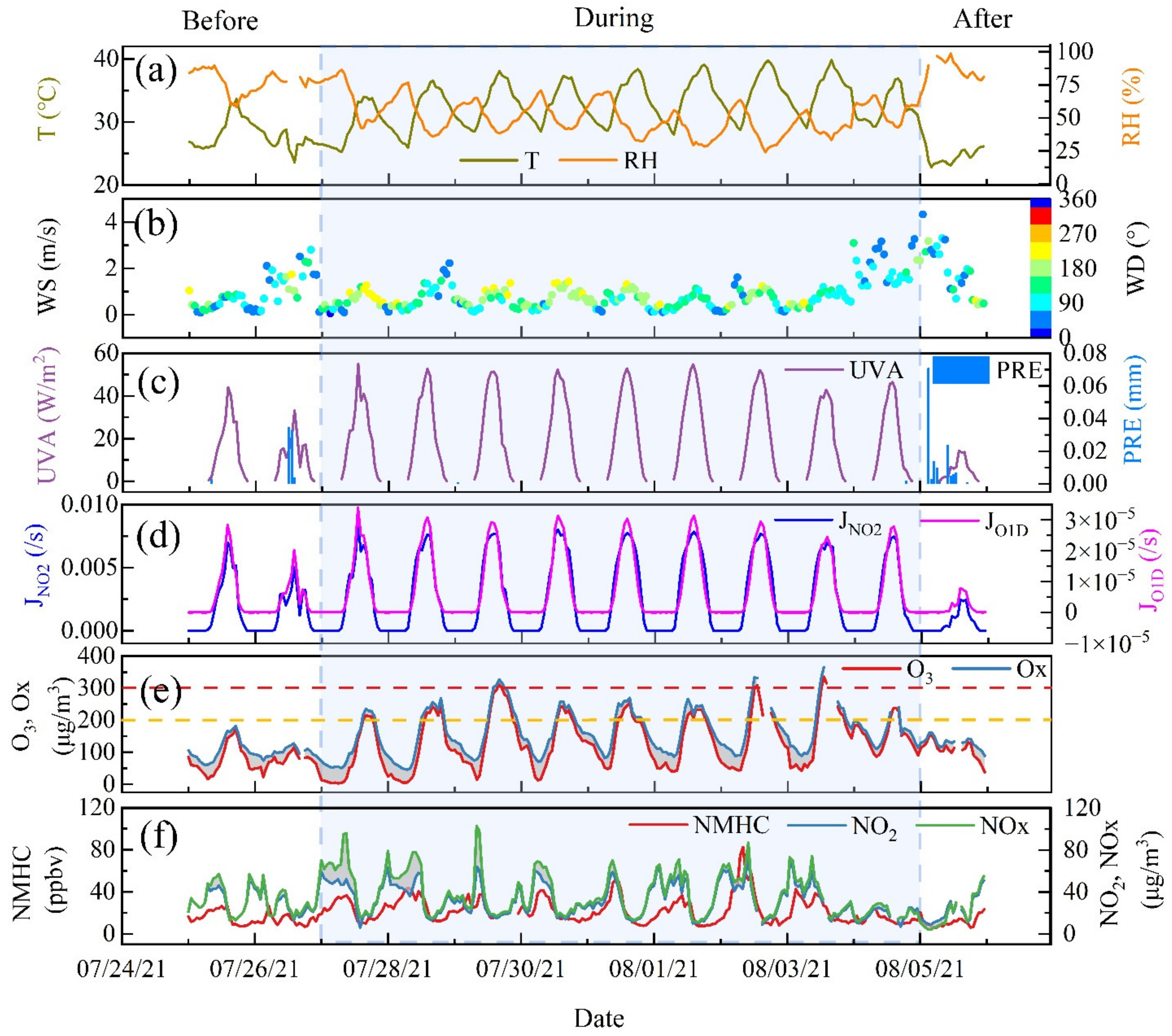
In this study, polluted days were classified according to the secondary standard of O3 hourly mean (O3 ≥ 200 μg/m3) formulated in China’s National Ambient Air Quality Standard [39]. During this pollution episode, O3 pollution in Chengdu lasted as long as 9 days, of which 6 days were mildly polluted (200 ≤ O3 < 300 μg/m3) and 3 days were moderately polluted (300 ≤ O3 < 400 μg/m3) (Figure 2e). Meteorological conditions showed that during this round of O3 pollution, sunny and hot weather continued, with high temperature (Tmax = 39.8 °C), low humidity (RHmin = 24.0%), and intense radiation (UVmax = 55.1 W/m2). The horizontal diffusion was basically dominated by southerly winds, and the WS slightly increased in a short time in the afternoon. The meteorological situations of this pollution episode were similar to the two O3 pollution events that occurred in Chengdu in summer 2017 [40], but this pollution was more serious and persistent. The inversion results of vertical diffusion data of aerosol lidar (Figure S2) showed that the height of the boundary layer was basically maintained above 2 km during the day, and the boundary layer decreased significantly at night, even less than 200 m.
From the perspective of the development stage of the pollution episode, there was no precipitation and calm wind during the whole O3 polluted period. In daytime, the sky opened more thoroughly and the atmospheric boundary layer was higher. Abundant levels of O3 precursors (NOx and NMHC) and intense ultraviolet intensity (UV) promoted the rapid O3 generation and sustained peak. Especially on 2 August, the concentrations of NO2 (76.0 μg/m3) and NMHC (82.4 ppbv) both reached the maximum value in the whole pollution episode. These directly pushed up the further increase in the O3 peak on 3 August, reaching the O3 maximum (335.0 μg/m3) for the entire process. In the later stage of pollution, the prominent WS and PRE reduced the O3 concentration, which played a role in removal of O3.
Generally speaking, the area with higher VOC concentrations levels usually has stronger atmospheric oxidation and is more likely to have ozone pollution events [41]. NOx further determines the overall and peak levels of ozone. This was illustrated by the time series plots of NOx versus O3 in Figure 2e,f. For example, the accumulation of high NOx concentration at night in 27 July–29 July and 1 August–3 August drove the O3 concentration to continue to rise in the daytime the next day. In Figure 2e, the gray shaded area (NO2 = Ox − O3, Ox means atmospheric oxidation capacity) during ozone pollution was significantly higher than that before and after pollution. This was precisely because NO2 significantly participates in O3 photochemical reactions, resulting in the production of high O3 concentration. At the same time, the NMHC mixing ratio and NOx concentration were also higher than those during the clean period, especially the gray shadow between NOx and NO2 (NO = NOx − NO2) increased significantly. The NO2 generated by the reaction of NO with VOCs photolysis products (HO2 and RO2 radicals) was further reacted to generate O3, indicating that this O3 pollution episode was accompanied by high concentrations of O3 precursors’ substances participating in the reaction.
3.1.2. Diurnal and Nocturnal Variation
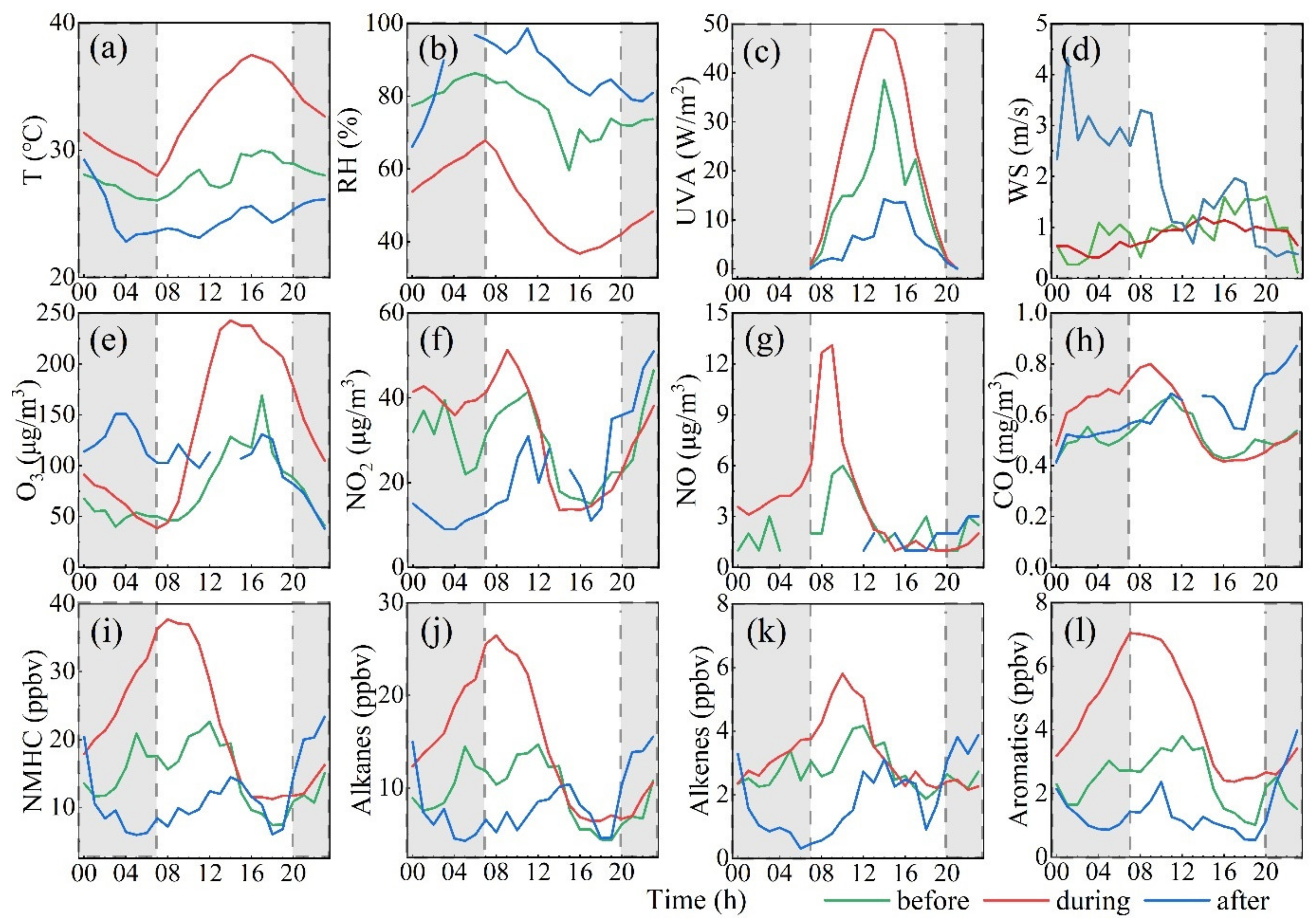
Figure 3 and Table 1 show the daily variation and average values of meteorological parameters and pollutants concentration before, during, and after O3 pollution over the observation period. The diurnal variation of O3 was unimodal (Figure 3e), indicating the same variation trend as the diurnal variation of temperature (Figure 3a), and a symmetric variation trend with RH, NO2, NO, CO, and VOC groups (Figure 3b,f–l). This reflected the apparent periodic variation between the precursor and its secondary contaminants.
In this study, 7:00–20:00 (CNST) was defined as daytime, and 21:00–6:00 (CNST) was defined as nighttime. O3 continued to oxidize NO at night, resulting in the gradual consumption of O3. Therefore, the concentration of O3 had a low value at sunrise. In the early morning, the light was weak, the photolysis rate of NO2 was slow, and O3 had just begun to accumulate. Between 7:00–10:00, human activities led to a large amount of VOCs and NOx entering the atmospheric environment, providing sufficient reaction precursors. With the increase of temperature, the solar radiation intensity increases. Under the irradiation of sunlight, the photochemical reaction became strong, and O3 showed a rapid upward trend. The O3 concentration peak value appeared around 14:00–17:00, while the NO2, CO, and VOC groups reached the minimum value. During the polluted period, the time of O3 concentration reaching the peak shifted forward, which might be due to the forward shift of radiation intensity and wind speed peaks, resulting in O3 concentration starting to fluctuate and decrease after 14:00. The peak values of O3 in the daytime were 169.0 μg/m3 (before the pollution), 242.8 μg/m3 (during the pollution), and 131.0 μg/m3 (after the pollution) in the three stages, respectively.
The mean values of NMHC before, during, and after the pollution were 15.0 ppbv, 21.7 ppbv, and 12.2 ppbv, respectively. During the polluted period, concentration of VOCs increased significantly. Alkanes, alkenes, and aromatics at different periods showed similar daily patterns to NMHC at each stage. Before the pollution, they all showed a bimodal shape, peaking at 5:00 and 12:00. Different from this, previous work in Chengdu showed that O3 was unimodal before the pollution [42]. In this study, the minima between the double peaks might be caused by VOCs participating in large number of ozone photochemical reactions, and the consumption rate of precursors was significantly higher than the emission rate. As the chemical reaction continued, the precursors involved in the reaction tend to be saturated, and the rate of feedstock consumption slowed down, resulting in formation of the second peak. Subsequently, with the sun set, the UV intensity gradually decreased, and the photolysis conditions of photochemical reactions decreased. Each precursor entered the night accumulation stage, so the concentration of precursors gradually rose at night.
The changes of VOC groups during ozone pollution were different from those before pollution, and they only formed a peak during the daytime. This indicated that the amount of VOCs as precursors in the ozone photochemical reaction was sufficient, and the consumption was less than the emission, so the valley between the two peaks could not be formed. However, the slight differences in the time span of the three stages could not cause significant differences in precursors emissions. The increase of VOC concentrations was caused by the adverse meteorological conditions (high temperature, low humidity, intense radiation, slow wind) and the reduction of atmosphere environmental capacity. After the pollution, the concentration of VOC groups was significantly lower than the previous two stages and started to accumulate again at night. It indicated that a large amount of precipitation in a short period of time (Figure 2c, from 2:00 to 6:00 on 5 August) played an absolute role in the removal of pollution in this round.
To further study the effect of VOC concentration changes on O3, this study plotted the diurnal and nocturnal variation of key VOC species with higher concentration and stronger activity, as shown in Figure S3. The diurnal trends of most components were the same as those of NMHC. It is worth noting that the concentration of isoprene rose rapidly after sunrise, remained at a high level between 11:00–20:00, and then decreased rapidly after sunset. It was consistent with the diurnal variation characteristics of isoprene in Nanjing in summer [43]. It showed that light had a great influence on the concentration of isoprene, and it was also one of the direct evidences for strong atmospheric oxidation in Chengdu. On the whole, by comparing the changes of meteorological parameters and precursor concentrations in the three stages, it was found that the O3 exceedance process in Chengdu presented the following two characteristics: (1) The temperature and solar radiation increased significantly, and the RH and WS decreased significantly, showing a static weather pattern; (2) the concentrations of NOx and VOCs increased significantly.
3.2. PICs and Consumed Concentrations of VOCs
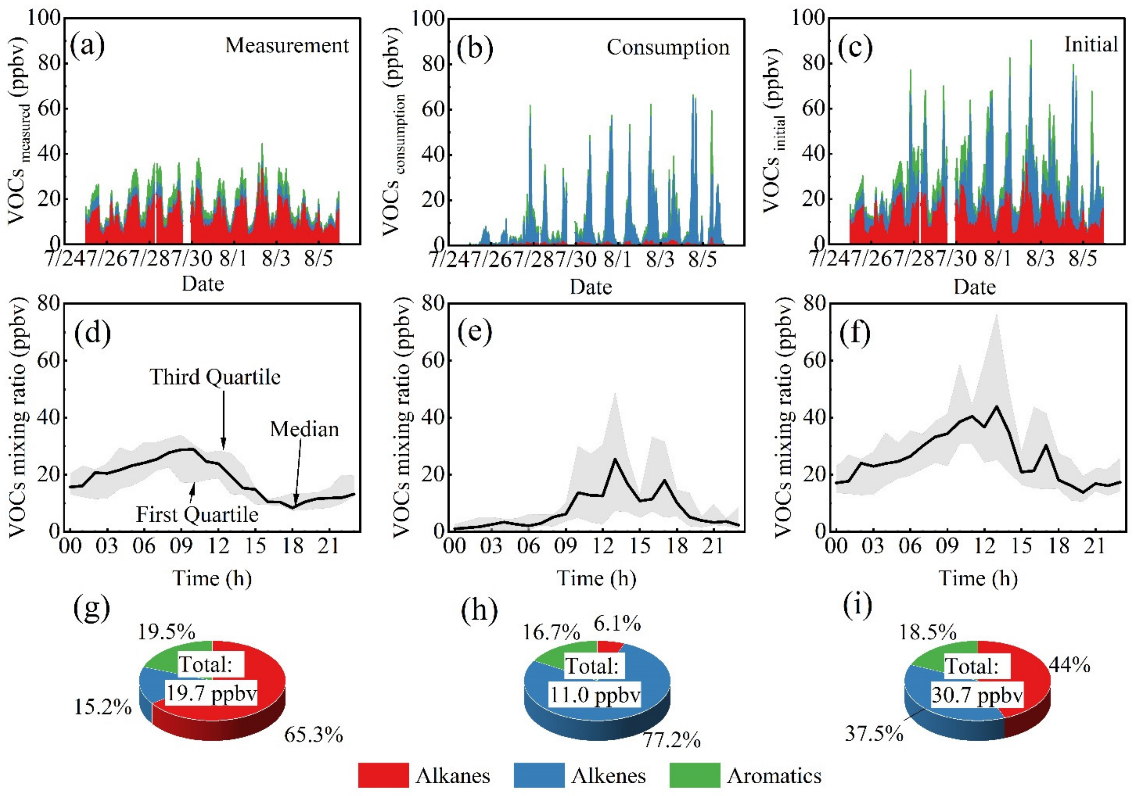
The time series (a–c), diurnal variations (d–f), and proportions (g–i) of VOCs measurement, consumption, and photochemical initial concentrations during the observation period are plotted in Figure 4. The variation range of VOCs measurement, consumption, and initial mixing ratio were 6.0–44.5 ppbv, 0.0–66.5 ppbv, and 6.2–90.2 ppbv, with average values of 19.7 ppbv, 11.0 ppbv, and 30.7 ppbv, respectively. The measured VOC concentrations during this observation period increased by about 5 ppbv compared to the concentration obtained at the same site in August 2019 [19]. Compared with before O3 pollution, the consumption concentration of VOCs during the polluted period was greatly enhanced, indicating that the photochemical aging rate at Chengdu urban area was faster during the polluted period. Previous studies might have seriously underestimated the concentration of VOCs in O3-heavy pollution days in Chengdu. The ratio of PICs to measured concentration varied from 1.0 to 9.5 (Figure S4). The ratios of PICs to measured concentration for all alkanes and partial aromatics were between 1.0 and 2.0, with larger ratios for alkenes and other aromatics, especially isoprene (9.5). This result was similar to the study in summer in Beijing [30], and species with high reactivity and low mixing ratio would have larger differences between measured concentrations and PICs. Therefore, when studying O3 pollution, the photochemical aging of VOC species with large OH reaction rate constants was worth exploring.
In this study, the maximum and minima values of measured VOC concentrations appeared at 10:00 and 18:00, respectively, which was delayed compared with the studies in Chengdu and Wuhan in the summer of 2018 [22,44]. This was different from the previous observation that VOCs presented peak values in the morning and evening at Beijing [10,45]. PICs had been increasing since the night, with double peaks appearing at 13:00 and 17:00, indicating that the emission had been enhanced at these two time points, which might be related to alkenes such as 1-pentene and isoprene (Figure S3). The mixing ratio of consumed VOCs increased significantly in daytime, the positions of the double peaks were the same as that of PICs, and there were almost no VOCs consumed at night. It showed that temperature and solar radiation greatly affected the photochemical aging process of VOCs. This result was different from that found in Beijing where PICs and consumed VOCs had only one peak during the daytime [10], which might be caused by the difference in emission of precursors between the two regions.
From the measured VOCs’ mixing ratio, alkanes accounted for a very high proportion, exceeding 60%, followed by aromatics (19.5%) and alkenes (15.2%). In the calculated PICs, the proportion of alkanes dropped to 44.0%, and the proportion of alkenes increased to 37.5%. It indicated that more alkenes were released into the air in the initial stage of emission. The proportion of alkenes in the consumption of VOCs’ mixing ratio reached 77.2%. Because the reaction rate constants of OH with alkanes were small, the consumption of alkanes (6.1%) with OH was less than those of alkenes and aromatics (77.2% and 16.7%). Therefore, the concentration of alkanes in urban areas is always higher during monitoring [19,42,46]. When considering the photochemical reactions of VOC species, all the VOC concentrations we observed were underestimated, especially alkenes.
3.3. VOCs Reactivity Characteristics
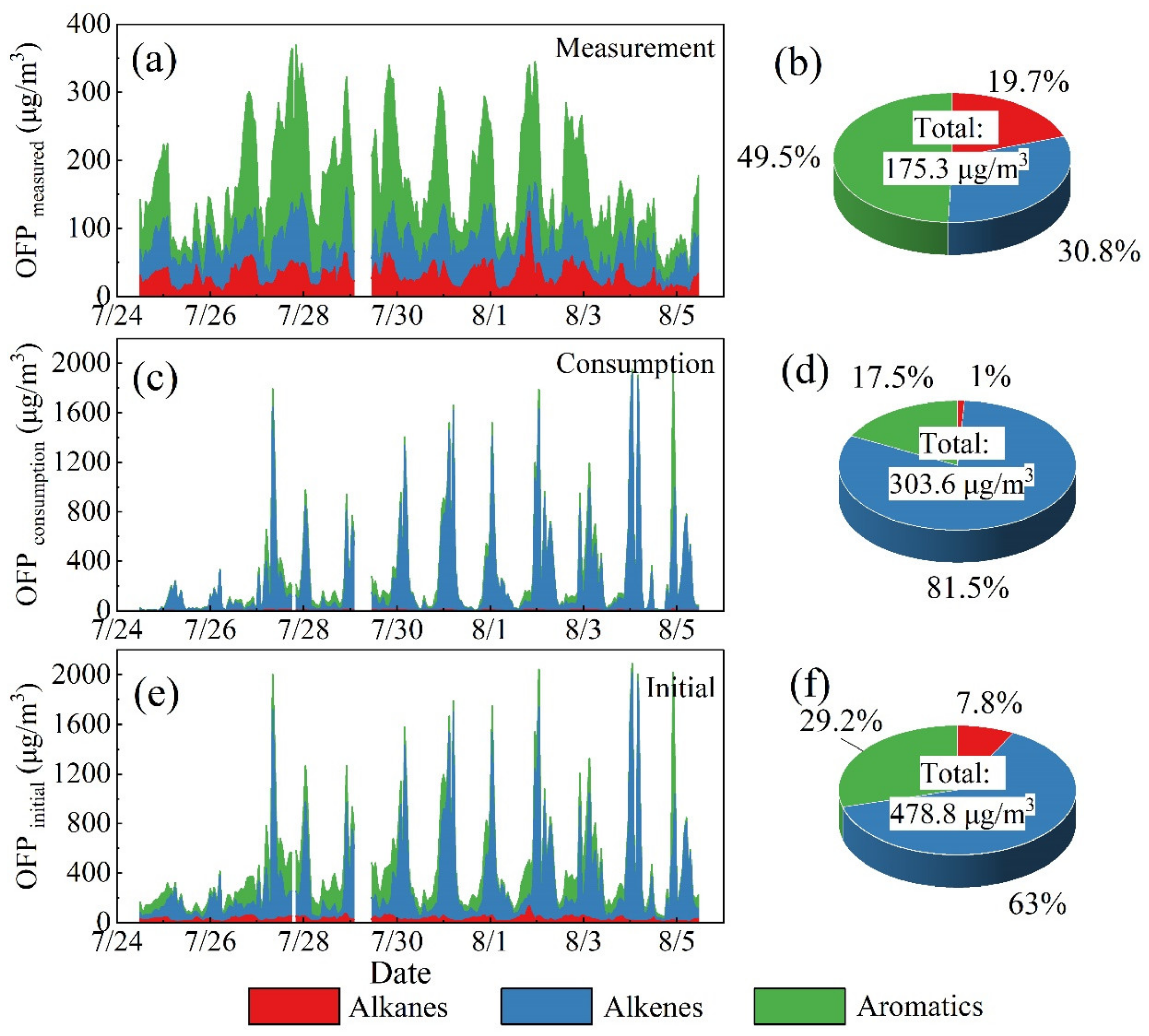
Different VOC species have different abilities to affect ozone generation due to their different activities. The time series and proportion of OFP of each VOC group during the observation period are shown in Figure 5. We calculated the mean OFP of VOCs based on measurement (OFPm), consumption (and OFPc), and initial concentration (OFPPICs) to be 175.3 μg/m3, 303.6 μg/m3, and 478.8 μg/m3, with fluctuations ranging from 39.9–369.7 μg/m3, 0.1–1970.6 μg/m3, and 48.1–2094.2 μg/m3, respectively. A previous study in Chengdu urban area showed that the average value of OFP was 338.7 μg/m3 [22], which was close to twice the estimated concentration of VOCs measured this time. The time series trend of OFP was similar to that of VOC mixing ratio, but the contributions of alkanes, alkenes, and aromatics were quite different. The mixing ratio of alkanes was the highest in both the measurement and the initial concentration, but due to the MIR values of alkanes being relatively small, their contribution to OFPm and OFPPICs was only 19.7% and 7.8%. Aromatics accounted for the largest proportion in OFPm (49.5%), which was significantly different from OFPc and OFPPICs. Alkenes accounted for 30.8% and 63.0% in OFPm and OFPPICs, and even increased to 81.5% in OFPc. It could be clearly seen that the O3 composition calculated using the consumed VOCs and PICs was dominated by alkenes. Alkenes had great potential in O3 formation in Chengdu, followed by aromatics and alkanes.
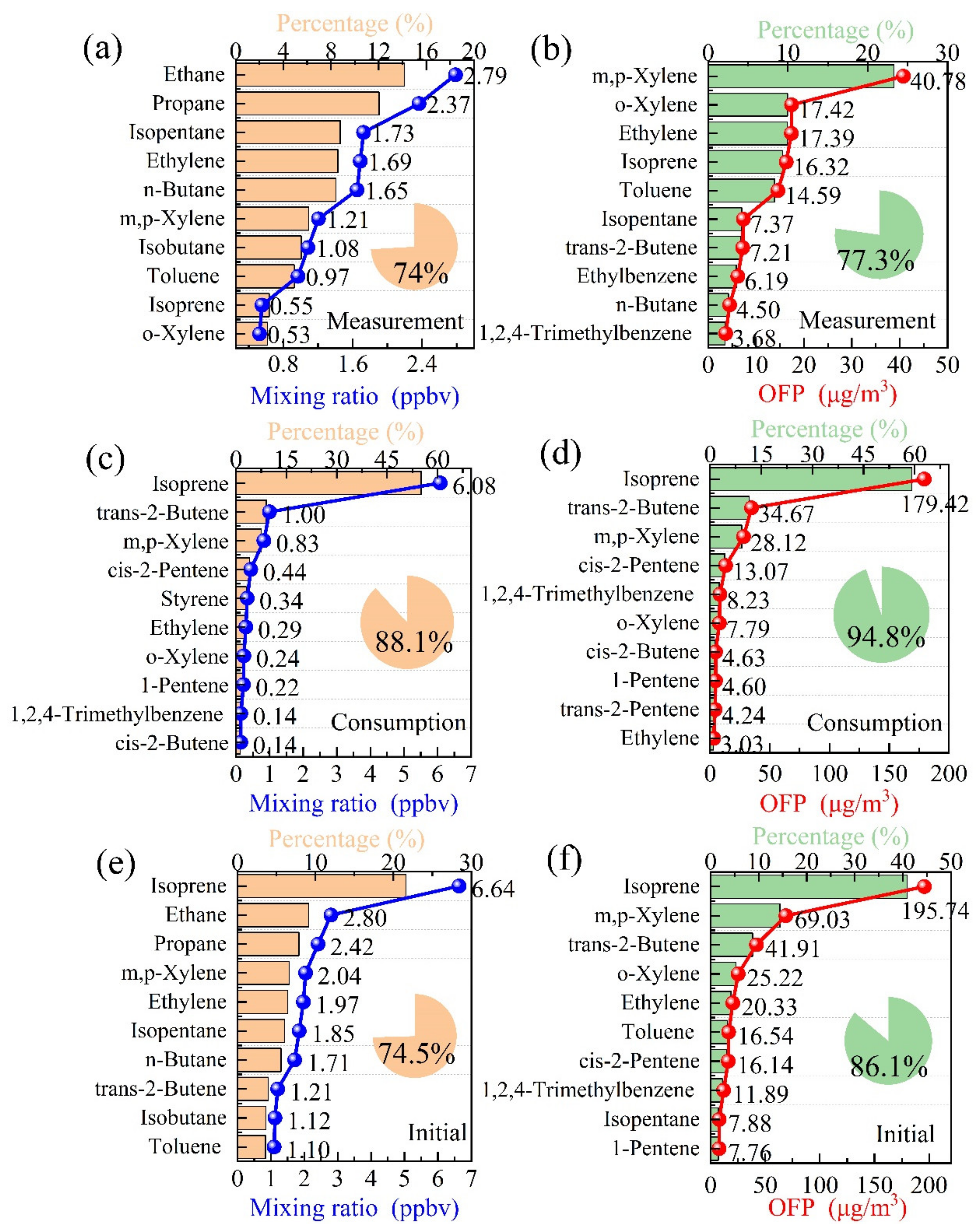
At the same time, we also ranked the top ten VOC species in terms of concentration and OFP during the observation period (Figure 6). The concentrations and OFP values of specific VOC species can be queried in Table S1. Among the measured VOCs, the top three were ethane (2.79 ppbv, 14.1%), propane (2.37 ppbv, 12.0%), and isopentane (1.73 ppbv, 8.8%), which fully demonstrated that alkanes occupy the largest component of the VOCs detected. The top 10 components in PICs were the same as six species in the measured VOCs, only the ordering was changed. Especially for isoprene, its mixing ratio (measured: 0.55 ppbv; initial: 6.64 ppbv) and proportion (measured: 2.8%; initial: 23.3%) were significantly increased. Unlike VOCs consumption ranking, the top ten species were all alkenes and aromatics. The top ten species contributed more than 70% to the measured, consumed, and initial VOC concentrations, and even accounted for 88.1% of the consumed VOCs.
Among the top ten OFP contributors, isoprene accounted for a much higher proportion of OFPPICs and OFPc than other species (40.9% and 59.1%, respectively). The contribution value to OFPPICs was slightly higher than that reported in Beijing (27.7%) [10]. Isoprene acts as a marker of biogenic volatile organic compounds, suggesting that biogenic emissions might play an important role in the formation of ground-level ozone in Chengdu. In addition, m,p-xylene, o-xylene, ethylene, and trans-2-butene also showed high photochemical reactivity and contributed most of the OFP, which was similar to the previous studies in Chengdu [22,42]. It indicated that solvent usage and gasoline vehicles emission had important contributions to the formation of O3. The top ten species accounted for 77.3%, 94.8%, and 86.1% of OFPm, OFPc, and OFPPICs, respectively. Therefore, the key active compounds in the formation of O3 in this region could be better identified using OFPc than OFPm [13]. It could be seen that the control and emission reduction of key dominant compounds could have a positive impact on the control of near-ground ozone.
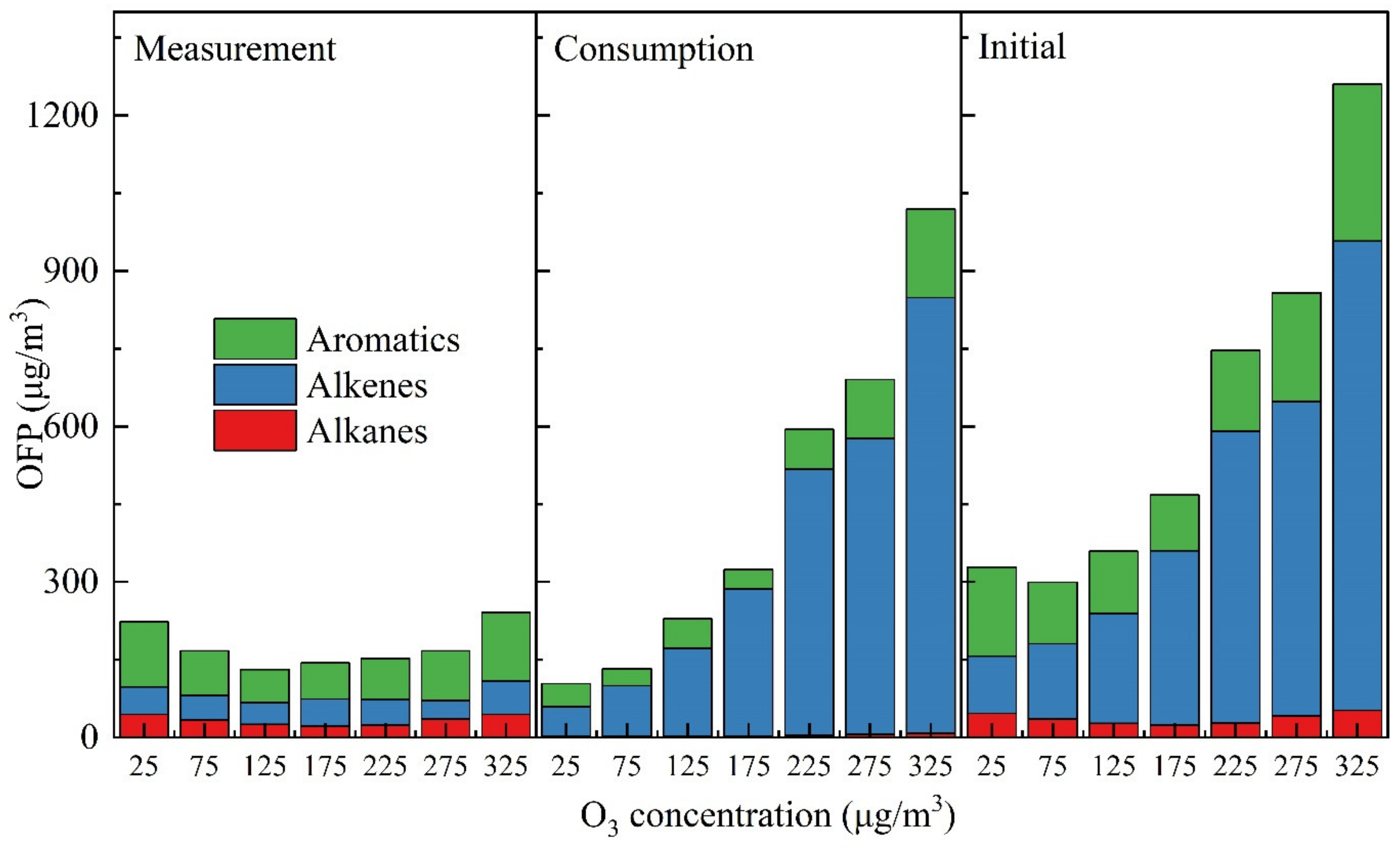
We divided the concentration of O3 into 50 μg/m3 intervals and discussed the change of OFP with the concentration of O3 (Figure 7). The OFPm of alkanes, alkenes, and aromatics were negatively correlated with O3 concentration below 175 μg/m3 and positively correlated when it was above 175 μg/m3. It showed that in the 0–175 μg/m3 stage, with the generation of ozone, the amount of remaining VOCs was less. At this stage, reducing the concentration of VOCs could not achieve ozone formation reduction. Aromatics and alkanes in OFPPICs and OFPc also had similar changing rules. Except at very low concentration of O3 (O3 < 75 μg/m3), OFPPICs and OFPc of alkenes had a stronger positive response to O3 concentration. Therefore, it is more appropriate to use OFP based on PICs or consumption concentrations to estimate O3 pollution, because it can better reflect the true potential of VOCs to form O3.
3.4. O3-VOC-NOx Relations
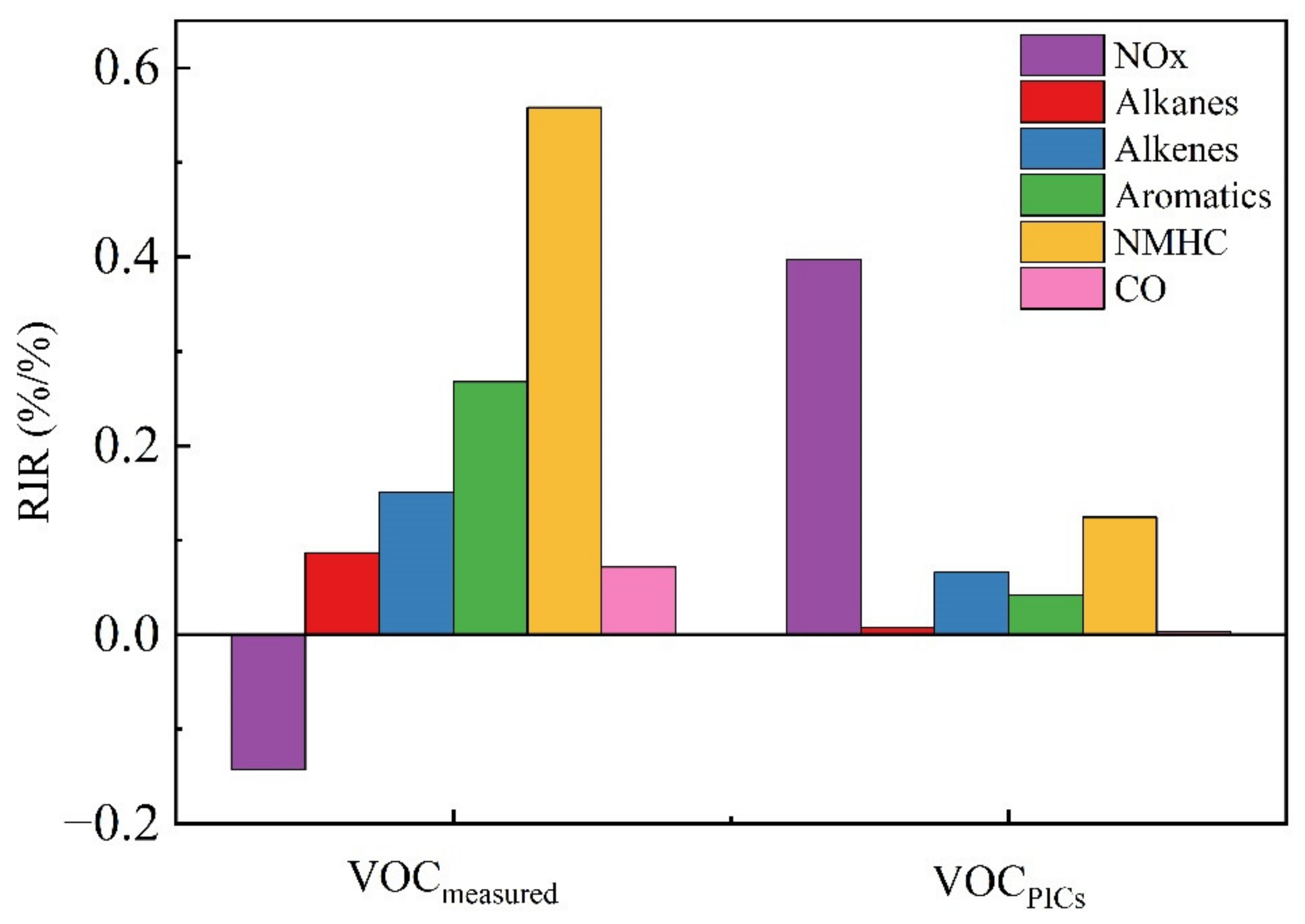
RIR is a parameter commonly used to describe the reactivity of O3 precursors. The absolute value of RIR represented the strength of sensitivity, and the positive and negative values indicated whether they promoted or inhibited the generation of O3 [47]. In this study, the monitored concentrations of VOCs (VOCm, defined as scenario 1) and PICs (VOCPICs, defined as scenario 2) were used as the input benchmark scenarios, respectively, and the concentrations of various precursors were reduced by 15% for the simulation of the OBM-MCM model. Isoprene was a typical natural-source VOC, and its concentration was kept constant when reducing alkenes and NMHC. The RIR values were calculated and plotted to obtain Figure 8.
The RIR values of the two scenarios were very different. Except for NOx in Scenario 1, RIRs of all precursors were greater than 0, and abatement of them could suppress the formation of O3. This means that when we used the monitoring values of VOCs to study ozone pollution, the generation of ozone was completely controlled by VOCs and exhibited the adverse effect of NOx reduction. The VOC group with stronger chemical activity (larger OFP) had a greater impact on ozone formation, and the absolute value of RIR should also be larger. The RIR values of alkanes, alkenes, and aromatics in both scenarios were in good agreement with their OFPs (Figure 5). The RIR of aromatics in the VOC sub-groups of Scenario 1 was the largest (0.27 %/%), which indicated that its reduction was the most effective for ozone pollution control in Chengdu. In the research of urban areas, it had been believed that NOx concentration was high and VOC concentration was low, and most urban areas were under the VOC-limited regime [21,48,49]. However, in this study, the RIRs of the three types of VOCs and CO in Scenario 2 were very small, which indicated that the impact of their emission reductions on ozone pollution control could be basically ignored. The RIR of NOx was the largest (0.40 %/%), indicating that when PICs of VOCs were considered, the sensitivity shifted significantly to the NOx-limited regime. During the ozone polluted period, due to the more intense photochemical reaction, the VOC concentrations we monitored consumed a lot compared with the initial emission concentration. When the actual concentration of VOCs was higher, NOx emission reduction had a certain effect. Our results suggested that it might be more reasonable to use PICs values rather than measurements to assess the sensitivity of O3 generation. This was consistent with the findings in Beijing [10].
We summarized the simulation results of the OBM carried out at the urban area of Chengdu (Table 2). It can be found that the previous studies generally believed that the urban area belongs to the VOC-limited regime, and the active VOC species were mainly alkenes [21,23,24]. In this study, the same results were obtained when VOC monitoring values were used, but the active species were changed to aromatics. Because the amount of VOCs consumed could not be ignored, it made more sense to estimate the initial concentration of VOCs. When using PICs of VOCs, Chengdu urban area was under the transition regime of VOCs and NOx and was more inclined to be NOx-limited. Therefore, in the O3 polluted period, moderate reduction of NOx had a better effect.
4. Conclusions
VOCs would be quickly consumed by oxidations in the condition of high temperature and intense radiation. In order to explore the influence of VOC consumption during the formation of O3, we selected an O3-heavy pollution episode from 25 July to 5 August, 2021 for analysis. The variation characteristics of pollutant concentrations before, during, and after pollution were discussed. During the polluted period, it was under high temperature (32.9 °C), intense radiation (23.9 W/m2), low humidity (50.8%), and slow wind (0.8 m/s), presenting stable weather. Meanwhile, the concentrations of NOx and various VOC species increased significantly, which was mainly attributed to the adverse meteorological conditions rather than the change of emission intensity. Comparing with the clean period, the consumption concentration of VOCs during the polluted period was greatly enhanced, especially the alkenes with strong reactivity. Previous studies might have seriously underestimated the concentration of VOCs in O3-heavy pollution days in Chengdu.
We calculated OFPm, OFPc, and OFPPICs based on the measured concentration and photochemical initial concentrations of VOCs. The proportion of aromatics contributing to OFPm was the largest, which was different from the other two. The contribution rates of alkenes and aromatics to OFPPICs were 63.0% and 29.2%, respectively. The key species affecting O3 formation were isoprene, m,p-xylene, o-xylene, ethylene, and trans-2-butene, indicating that biogenic emission, solvent usage, and gasoline vehicle exhaust played important roles in O3 formation. Isoprene, in particular, accounted for between 40–60% in OFPc and OFPPICs. Therefore, using OFPPICs or OFPc to estimate O3 pollution could reflect a proper potential of O3 formation through VOC oxidations.
The emission reduction simulation was carried out depending on measured VOC concentrations, and the urban area of Chengdu was under the VOC-limited regime. When PICs was used, it was changed to a transition regime. This indicated that when the actual concentration of VOCs in the environment was higher, the reduction of NOx had a significant effect, and the reduction of strongly active VOC species was also effective. It might be more reasonable to use PICs values rather than measurements to assess the sensitivity of O3 generation. In addition, it should be noted that it is necessary to evaluate the relative proportions, costs, and benefits of O3-VOC-NOx sensitivity continually based on long-term monitoring to optimize O3 pollution prevention and control measures.
Supplementary Materials
The following supporting information can be downloaded at: https://www.mdpi.com/article/10.3390/atmos13101534/s1, Figure S1: Scatterplot between m,p-xylene and ethylbenzene (left). Diurnal variation of m,p-xylene/ethylbenzene mixing ratio (right).; Figure S2: Inversion map of vertical diffusion data from aerosol lidar. Figure S3: Diurnal and nocturnal variation of key VOC species (formaldehyde (a), alkanes (b–d), alkenes (e–h), aromatics (i–k)) before (25 July–26 July), during (27 July–4 August), and after (5 August) the pollution. Figure S4: The ratios of initial/measured concentration of VOCs. Table S1: The contributions of VOCs to OFP at Chengdu.
Author Contributions
Conceptualization, H.L. and N.W.; methodology, N.W.; software, H.L. and D.C.; validation, H.L., N.W. and D.C.; formal analysis, H.L.; investigation, D.S.; resources, Q.T. and D.S.; data curation, H.L.; writing–original draft preparation, H.L. and N.W.; writing–review and editing, H.L. and N.W.; visualization, H.L., N.W. and D.C.; supervision, Q.T. and F.H.; project administration, D.S. and F.H.; funding acquisition, N.W. and D.S. All authors have read and agreed to the published version of the manuscript.
Funding
This research was funded by National Natural Science Foundation of China, grant number 42175124, and Chengdu Science and Technology Bureau, grant number 2020-YF09-00051-SN.
Institutional Review Board Statement
Not applicable.
Informed Consent Statement
Not applicable.
Acknowledgments
We are grateful for financial support from the National Natural Science Foundation of China, grant number 22276128 and 42175124, and Chengdu Science and Technology Bureau, grant number 2020-YF09-00051-SN. We would also like to show deep thankfulness to the reviewers and editors who have contributed valuable comments to improve the quality of the paper.
Conflicts of Interest
The authors declare no conflict of interest.
References
- Felzer, B.S.; Cronin, T.; Reilly, J.M.; Melilloa, J.M.; Wang, X.D. Impacts of ozone on trees and crops. C. R. Geosci. 2007, 339, 784–798. [Google Scholar] [CrossRef]
- Zhu, X.K.; Feng, Z.Z.; Sun, T.F.; Liu, X.C.; Tang, H.Y.; Zhu, J.G.; Guo, W.S.; Kobayashi, K. Effects of elevated ozone concentration on yield of four Chinese cultivars of winter wheat under fully open-air field conditions. Glob. Change Biol. 2011, 17, 2697–2706. [Google Scholar] [CrossRef]
- Sun, J.; Shen, Z.X.; Zhang, Y.; Zhang, Z.; Zhang, Q.; Zhang, T.; Niu, X.Y.; Huang, Y.; Cui, L.; Xu, H.M.; et al. Urban VOC profiles, possible sources, and its role in ozone formation for a summer campaign over Xi’an, China. Environ. Sci. Pollut. Res. 2019, 26, 27769–27782. [Google Scholar] [CrossRef] [PubMed]
- Huang, Y.S.; Hsieh, C.C. Ambient volatile organic compound presence in the highly urbanized city: Source apportionment and emission position. Atmos. Environ. 2019, 206, 45–59. [Google Scholar] [CrossRef]
- Zheng, H.; Kong, S.; Chen, N.; Niu, Z.; Zhang, Y.; Jiang, S.; Yan, Y.; Qi, S. Source apportionment of volatile organic compounds: Implications to reactivity, ozone formation, and secondary organic aerosol potential. Atmos. Res. 2021, 249, 105344. [Google Scholar] [CrossRef]
- Li, Y.D.; Yin, S.S.; Yu, S.J.; Yuan, M.H.; Dong, Z.; Zhang, D.; Yang, L.M.; Zhang, R.Q. Characteristics, source apportionment and health risks of ambient VOCs during high ozone period at an urban site in central plain, China. Chemosphere 2020, 250, 126283. [Google Scholar] [CrossRef]
- Deng, Y.Y.; Li, J.; Li, Y.Q.; Wu, R.R.; Xie, S.D. Characteristics of volatile organic compounds, NO2, and effects on ozone formation at a site with high ozone level in Chengdu. J. Environ. Sci. 2019, 75, 334–345. [Google Scholar] [CrossRef]
- Warneke, C.; De Gouw, J.A.; Goldan, P.D.; Kuster, W.C.; Williams, E.J.; Lerner, B.M.; Jakoubek, R.; Brown, S.S.; Stark, H.; Aldener, M.; et al. Comparison of daytime and nighttime oxidation of biogenic and anthropogenic VOCs along the New England coast in summer during New England Air Quality Study 2002. J. Geophys. Res.: Atmos. 2004, 109, D10309. [Google Scholar] [CrossRef]
- Gao, Y.Q.; Li, M.; Wan, X.; Zhao, X.W.; Wu, Y.; Liu, X.X.; Li, X. Important contributions of alkenes and aromatics to VOCs emissions, chemistry and secondary pollutants formation at an industrial site of central eastern China. Atmos. Environ. 2021, 244, 117927. [Google Scholar] [CrossRef]
- Zhan, J.L.; Feng, Z.M.; Liu, P.F.; He, X.W.; He, Z.M.; Chen, T.Z.; Wang, Y.F.; He, H.; Mu, Y.J.; Liu, Y.C. Ozone and SOA formation potential based on photochemical loss of VOCs during the Beijing summer. Environ. Pollut. 2021, 285, 117444. [Google Scholar] [CrossRef]
- He, Z.; Wang, X.; Ling, Z.; Zhao, J.; Guo, H.; Shao, M.; Wang, Z. Contributions of different anthropogenic volatile organic compound sources to ozone formation at a receptor site in the Pearl River Delta region and its policy implications. Atmos. Chem. Phys. 2019, 19, 8801–8816. [Google Scholar] [CrossRef]
- Yuan, B.; Hu, W.W.; Shao, M.; Wang, M.; Chen, W.T.; Lu, S.H.; Zeng, L.M.; Hu, M. VOC emissions, evolutions and contributions to SOA formation at a receptor site in eastern China. Atmos. Chem. Phys. 2013, 13, 8815–8832. [Google Scholar] [CrossRef]
- Shao, M.; Wang, B.; Lu, S.H.; Yuan, B.; Wang, M. Effects of Beijing Olympics Control Measures on Reducing Reactive Hydrocarbon Species. Environ. Sci. Technol. 2011, 45, 514–519. [Google Scholar] [CrossRef]
- Shi, G.M.; Yang, F.M.; Zhang, L.M.; Zhao, T.L.; Hu, J. Impact of Atmospheric Circulation and Meteorological Parameters on Wintertime Atmospheric Extinction in Chengdu and Chongqing of Southwest China during 2001–2016. Aerosol Air Qual. Res. 2019, 19, 1538–1554. [Google Scholar] [CrossRef]
- Bo, Y.; Cai, H.; Xie, S.D. Spatial and temporal variation of historical anthropogenic NMVOCs emission inventories in China. Atmos. Chem. Phys. 2008, 8, 7297–7316. [Google Scholar] [CrossRef]
- Hu, W.; Hu, M.; Hu, W.W.; Niu, H.Y.; Zheng, J.; Wu, Y.S.; Chen, W.T.; Chen, C.; Li, L.Y.; Shao, M.; et al. Characterization of submicron aerosols influenced by biomass burning at a site in the Sichuan Basin, southwestern China. Atmos. Chem. Phys. 2016, 16, 13213–13230. [Google Scholar] [CrossRef]
- Tao, J.; Gao, J.; Zhang, L.; Zhang, R.; Che, H.; Zhang, Z.; Lin, Z.; Jing, J.; Cao, J.; Hsu, S.C. PM2.5 pollution in a megacity of southwest China: Source apportionment and implication. Atmos. Chem. Phys. 2014, 14, 8679–8699. [Google Scholar] [CrossRef]
- Chen, D.Y.; Zhou, L.; Wang, C.; Liu, H.F.; Qiu, Y.; Shi, G.M.; Song, D.L.; Tan, Q.W.; Yang, F.M. Characteristics of ambient volatile organic compounds during spring O3 pollution episode in Chengdu, China. J. Environ. Sci. 2022, 114, 115–125. [Google Scholar] [CrossRef]
- Tan, Q.; Zhou, L.; Liu, H.; Feng, M.; Qiu, Y.; Yang, F.; Jiang, W.; Wei, F. Observation-Based Summer O3 Control Effect Evaluation: A Case Study in Chengdu, a Megacity in Sichuan Basin, China. Atmosphere 2020, 11, 1278. [Google Scholar] [CrossRef]
- Tan, Q.W.; Liu, H.F.; Xie, S.D.; Zhou, L.; Song, T.L.; Shi, G.M.; Jiang, W.J.; Yang, F.M.; Wei, F.S. Temporal and spatial distribution characteristics and source origins of volatile organic compounds in a megacity of Sichuan Basin, China. Environ. Res. 2020, 185, 109478. [Google Scholar] [CrossRef]
- Tan, Z.F.; Lu, K.D.; Jiang, M.Q.; Su, R.; Dong, H.B.; Zeng, L.M.; Xie, S.D.; Tan, Q.W.; Zhang, Y.H. Exploring ozone pollution in Chengdu, southwestern China: A case study from radical chemistry to O3-VOC-NOx sensitivity. Sci. Total Environ. 2018, 636, 775–786. [Google Scholar] [CrossRef] [PubMed]
- Xiong, C.; Wang, N.; Zhou, L.; Yang, F.M.; Qiu, Y.; Chen, J.H.; Han, L.; Li, J.J. Component characteristics and source apportionment of volatile organic compounds during summer and winter in downtown Chengdu, southwest China. Atmos. Environ. 2021, 258, 118485. [Google Scholar] [CrossRef]
- Han, L.; Chen, J.H.; Jiang, T.; Xu, C.X.; Li, Y.J.; Wang, C.H.; Wang, B.; Qian, J.; Liu, Z. Characteristics of O3 pollution and key precursors in Chengdu during spring. Environ. Sci. 2021, 42, 4611–4620. [Google Scholar] [CrossRef]
- Han, L.; Chen, J.H.; Jiang, T.; Xu, C.X.; Li, Y.J.; Wang, C.H.; Wang, B.; Qian, J.; Liu, Z. Sensitivity analysis of atmospheric ozone formation to its precursors in Chengdu with an observation based model. Acta Sci. Circumstantiae 2020, 40, 4092–4104. [Google Scholar] [CrossRef]
- Song, M.D.; Tan, Q.W.; Feng, M.; Qu, Y.; Liu, X.G.; An, J.L.; Zhang, Y.H. Source apportionment and secondary transformation of atmospheric nonmethane hydrocarbons in Chengdu, southwest China. J. Geophys. Res.-Atmos. 2018, 123, 9741–9763. [Google Scholar] [CrossRef]
- Carter, W.P.L. Updated maximum incremental reactivity scale and hydrocarbon bin reactivities for regulatory applications. Prepared for California Air Resources Board Contract No. 07–339. 19 January 2010. Available online: https://www.cert.ucr.edu/~carter/SAPRC.
- Carter, W.P.L. Development of a database for chemical mechanism assignments for volatile organic emissions. J. Air Waste Manage. Assoc. 2015, 65, 1171–1184. [Google Scholar] [CrossRef]
- Roberts, J.M.; Fehsenfeld, F.C.; Liu, S.C.; Bollinger, M.J.; Hahn, C.; Albritton, D.L.; Sievers, R.E. Measurements of Aromatic Hydrocarbon Ratios and Nox Concentrations in the Rural Troposphere-Observation of Air-Mass Photochemical Aging and Nox Removal. Atmos. Environ. 1984, 18, 2421–2432. [Google Scholar] [CrossRef]
- Parrish, D.D.; Stohl, A.; Forster, C.; Atlas, E.L.; Blake, D.R.; Goldan, P.D.; Kuster, W.C.; De Gouw, J.A. Effects of mixing on evolution of hydrocarbon ratios in the troposphere. J. Geophys. Res. Atmos. 2007, 112, D10S34. [Google Scholar] [CrossRef]
- Shao, M.; Lu, S.H.; Liu, Y.; Xie, X.; Chang, C.C.; Huang, S.; Chen, Z.M. Volatile organic compounds measured in summer in Beijing and their role in ground-level ozone formation. J. Geophys. Res. Atmos. 2009, 114, D00G06. [Google Scholar] [CrossRef]
- Han, D.M.; Wang, Z.; Cheng, J.P.; Wang, Q.; Chen, X.J.; Wang, H.L. Volatile organic compounds (VOCs) during non-haze and haze days in Shanghai: Characterization and secondary organic aerosol (SOA) formation. Environ. Sci. Pollut. Res. 2017, 24, 18619–18629. [Google Scholar] [CrossRef]
- Yuan, B.; Shao, M.; De Gouw, J.; Parrish, D.D.; Lu, S.H.; Wang, M.; Zeng, L.M.; Zhang, Q.; Song, Y.; Zhang, J.B.; et al. Volatile organic compounds (VOCs) in urban air: How chemistry affects the interpretation of positive matrix factorization (PMF) analysis. J. Geophys. Res. Atmos. 2012, 117, D24302. [Google Scholar] [CrossRef]
- Atkinson, R.; Arey, J. Atmospheric degradation of volatile organic compounds. Chem. Rev. 2003, 103, 4605–4638. [Google Scholar] [CrossRef] [PubMed]
- Jenkin, M.E.; Saunders, S.M.; Pilling, M.J. The tropospheric degradation of volatile organic compounds: A protocol for mechanism development. Atmos. Environ. 1997, 31, 81–104. [Google Scholar] [CrossRef]
- Saunders, S.M.; Jenkin, M.E.; Derwent, R.G.; Pilling, M.J. Protocol for the development of the Master Chemical Mechanism, MCM v3 (Part A): Tropospheric degradation of non-aromatic volatile organic compounds. Atmos. Chem. Phys. 2003, 3, 161–180. [Google Scholar] [CrossRef]
- Jenkin, M.E.; Saunders, S.M.; Wagner, V.; Pilling, M.J. Protocol for the development of the Master Chemical Mechanism, MCM v3 (Part B): Tropospheric degradation of aromatic volatile organic compounds. Atmos. Chem. Phys. 2003, 3, 181–193. [Google Scholar] [CrossRef]
- Wang, M.; Chen, W.T.; Zhang, L.; Qin, W.; Zhang, Y.; Zhang, X.Z.; Xie, X. Ozone pollution characteristics and sensitivity analysis using an observation-based model in Nanjing, Yangtze River Delta Region of China. J. Environ. Sci. 2020, 93, 13–22. [Google Scholar] [CrossRef]
- Li, J.; Zhai, C.Z.; Yu, J.Y.; Liu, R.L.; Li, Y.Q.; Zeng, L.M.; Xie, S.D. Spatiotemporal variations of ambient volatile organic compounds and their sources in Chongqing, a mountainous megacity in China. Sci. Total Environ. 2018, 627, 1442–1452. [Google Scholar] [CrossRef]
- GB 3095-2012; Ambient Air Quality Standards. Ministry of Ecology and Environment of the People’s Republic of China: Beijing, China, 29 February 2012.
- Yang, X.Y.; Wu, K.; Wang, H.L.; Liu, Y.M.; Gu, S.; Lu, Y.Q.; Zhang, X.L.; Hu, Y.S.; Ou, Y.H.; Wang, S.G.; et al. Summertime ozone pollution in Sichuan Basin, China: Meteorological conditions, sources and process analysis. Atmos. Environ. 2020, 226, 117392. [Google Scholar] [CrossRef]
- Atkinson, R. Atmospheric chemistry of VOCs and NOx. Atmos. Environ. 2000, 34, 2063–2101. [Google Scholar] [CrossRef]
- Song, M.; Feng, M.; Li, X.; Tan, Q.; Song, D.; Liu, H.; Dong, H.; Zeng, L.; Lu, K.; Zhang, Y. Causes and sources of heavy ozone pollution in Chengdu. China Environ. Sci. 2022, 42, 1057–1065. [Google Scholar] [CrossRef]
- Xu, Z.N. Observation Based Study of VOCs and Their Influence of on Ozone and Secondary Organic Aerosol formation in the Western YRD Region, China. Ph.D. Thesis, Nanjing University, Nanjing, China, 2019. [Google Scholar]
- Zhu, J.; Cheng, H.; Peng, J.; Zeng, P.; Wang, Z.; Lyu, X.; Guo, H. O3 photochemistry on O3 episode days and non-O3 episode days in Wuhan, Central China. Atmos. Environ. 2020, 223, 117236. [Google Scholar] [CrossRef]
- Li, J.; Wu, R.; Li, Y.; Hao, Y.; Xie, S.; Zeng, L. Effects of rigorous emission controls on reducing ambient volatile organic compounds in Beijing, China. Sci. Total Environ. 2016, 557, 531–541. [Google Scholar] [CrossRef] [PubMed]
- Cai, C.J.; Geng, F.H.; Tie, X.X.; Yu, Q.O.; An, J.L. Characteristics and source apportionment of VOCs measured in Shanghai, China. Atmos. Environ. 2010, 44, 5005–5014. [Google Scholar] [CrossRef]
- Cardelino, C.A.; Chameides, W.L. An Observation-Based Model for Analyzing Ozone Precursor Relationships in the Urban Atmosphere. J. Air Waste Manag. Assoc. 1995, 45, 161–180. [Google Scholar] [CrossRef] [PubMed]
- An, J.L.; Zou, J.N.; Wang, J.X.; Lin, X.; Zhu, B. Differences in ozone photochemical characteristics between the megacity Nanjing and its suburban surroundings, Yangtze River Delta, China. Environ. Sci. Pollut. Res. 2015, 22, 19607–19617. [Google Scholar] [CrossRef] [PubMed]
- Zhang, Y.; Xue, L.; Chen, T.; Shen, H.; Li, H.; Wang, W. Development history of Observation-Based Model (OBM) and its application and prospect in atmospheric chemistry studies in China. Res. Environ. Sci. 2022, 35, 621–632. [Google Scholar] [CrossRef]
Figure 1.
Schematic diagram of the observation location.

Figure 2.
Time series of meteorological parameters (a,b), UVA (c), photolysis rate constants (d), and pollutant concentrations (e,f) in Chengdu during the observation period. The blue shading shows the polluted period. Before: 25 July–26 July; during: 27 July–4 August; after: 5 August.
Figure 2.
Time series of meteorological parameters (a,b), UVA (c), photolysis rate constants (d), and pollutant concentrations (e,f) in Chengdu during the observation period. The blue shading shows the polluted period. Before: 25 July–26 July; during: 27 July–4 August; after: 5 August.

Figure 3.
Diurnal and nocturnal variation of meteorological parameters (a–d), gaseous pollutants (e–h), and NMHCs (i–l) before (25 July–26 July), during (27 July–4 August), and after (5 August) the O3 pollution. The gray shaded area indicates nighttime (daytime: 7:00–20:00 CNST; nighttime: 21:00–6:00 CNST).

Figure 4.
Time series (a–c), diurnal variation (d–f), and proportion (g–i) of VOCs measurement, consumption, and photochemical initial concentrations during the observation period. The gray areas in panels (d–f) represent the VOCs’ mixing ratio between 25% and 75% percentiles.
Figure 4.
Time series (a–c), diurnal variation (d–f), and proportion (g–i) of VOCs measurement, consumption, and photochemical initial concentrations during the observation period. The gray areas in panels (d–f) represent the VOCs’ mixing ratio between 25% and 75% percentiles.

Figure 5.
Time series (a,c,e) and proportions (b,d,f) of measurement, consumption, and photochemical initial concentrations of OFP during the observation period.
Figure 5.
Time series (a,c,e) and proportions (b,d,f) of measurement, consumption, and photochemical initial concentrations of OFP during the observation period.

Figure 6.
Mixing ratio (a,c,e) and OFP (b,d,f) of the top ten VOC species during the observation period.
Figure 6.
Mixing ratio (a,c,e) and OFP (b,d,f) of the top ten VOC species during the observation period.

Figure 7.
OFP of VOCs measured (left), consumed (middle), and initial (right) concentrations at different O3 concentration segments during the observation period.
Figure 7.
OFP of VOCs measured (left), consumed (middle), and initial (right) concentrations at different O3 concentration segments during the observation period.

Figure 8.
RIR values for NOx, Alkanes, Alkenes, Aromatics, NMHC, and CO.


Table 1.
Mean value of meteorological, O3 concentration, and ambient air pollutants before, during, and after polluted period at monitoring site.
Table 1.
Mean value of meteorological, O3 concentration, and ambient air pollutants before, during, and after polluted period at monitoring site.
| Before (2 Days) | During (9 Days) | After (1 Day) | |
|---|---|---|---|
| T (°C) | 27.9 ± 2.2 | 32.9 ± 3.5 | 24.8 ± 1.6 |
| RH (%) | 77.3 ± 23.0 | 50.8 ± 13.2 | 85.5 ± 25.4 |
| WS (m/s) | 0.9 ± 0.7 | 0.8 ± 0.6 | 1.9 ± 1.1 |
| UVA (W/m2) | 14.5 ± 11.9 | 23.9 ± 18.4 | 5.6 ± 4.7 |
| JNO2 (/s) | 1.6×10⁻³ ± 2.0×10⁻³ | 2.6×10⁻³ ± 3.0×10⁻³ | 6.2×10⁻⁴ ± 8.2×10⁻⁴ |
| JO1D (/s) | 4.7×10⁻⁶ ± 7.2×10⁻⁶ | 7.4×10⁻⁶ ± 1.0×10⁻⁵ | 1.5×10⁻⁶ ± 2.5×10⁻⁶ |
| O3 (μg/m3) | 74.4 ± 37.0 | 132.3 ± 84.0 | 107.8 ± 40.4 |
| Ox (μg/m3) | 103.9 ± 32.3 | 162.6 ± 77.1 | 129.3 ± 39.9 |
| NO (μg/m3) | 2.7 ± 2.0 | 3.9 ± 4.7 | 1.8 ± 1.0 |
| NO2 (μg/m3) | 29.3 ± 11.1 | 32.4 ± 16.3 | 21.8 ± 12.9 |
| NOx (μg/m3) | 31.9 ± 13.3 | 38.3 ± 21.1 | 20.4 ± 15.5 |
| CO (mg/m3) | 0.5 ± 0.1 | 0.6 ± 0.2 | 0.6 ± 0.2 |
| Alkanes (ppbv) | 10.0 ± 3.9 | 14.0 ± 6.2 | 8.7 ± 3.4 |
| Alkenes (ppbv) | 2.6 ± 1.0 | 3.3 ± 1.4 | 2.1 ± 1.1 |
| Aromatics (ppbv) | 2.4 ± 1.3 | 4.4 ± 2.4 | 1.4 ± 0.8 |
| NMHC (ppbv) | 15.0 ± 5.7 | 21.7 ± 9.1 | 12.2 ± 5.0 |
Table 2.
Summary of the OBM studies in O3 formation regime at urban areas of Chengdu.
| Location | Time | VOC | Chemical Mechanism | O3 Formation Mechanism | Active VOC Species | Ref. |
|---|---|---|---|---|---|---|
| Wuhou | 3 September 2016–2 October 2016 | Measured | RACM2 | VOC-limited | Alkenes | [21] |
| Wuhou | 2 April 2018–30 April 2018 | Measured | CB05 | VOC-limited | Alkenes | [23] |
| Wuhou | 1 April 2019–31 August 2019 | Measured | CB05 | VOC-limited | AVOCs* | [24] |
| Qingyang | 25 July 2021–5 August 2021 | Measured | MCM v3.3.1 | VOC-limited | Aromatics | This study |
| PICs | transition | Alkenes |
* AVOCs: artificial VOCs.
Publisher’s Note: MDPI stays neutral with regard to jurisdictional claims in published maps and institutional affiliations. |
© 2022 by the authors. Licensee MDPI, Basel, Switzerland. This article is an open access article distributed under the terms and conditions of the Creative Commons Attribution (CC BY) license (https://creativecommons.org/licenses/by/4.0/).
Share and Cite
MDPI and ACS Style
Liu, H.; Wang, N.; Chen, D.; Tan, Q.; Song, D.; Huang, F. How Photochemically Consumed Volatile Organic Compounds Affect Ozone Formation: A Case Study in Chengdu, China. Atmosphere 2022, 13, 1534. https://doi.org/10.3390/atmos13101534
AMA Style
Liu H, Wang N, Chen D, Tan Q, Song D, Huang F. How Photochemically Consumed Volatile Organic Compounds Affect Ozone Formation: A Case Study in Chengdu, China. Atmosphere. 2022; 13(10):1534. https://doi.org/10.3390/atmos13101534
Chicago/Turabian StyleLiu, Hefan, Ning Wang, Dongyang Chen, Qinwen Tan, Danlin Song, and Fengxia Huang. 2022. "How Photochemically Consumed Volatile Organic Compounds Affect Ozone Formation: A Case Study in Chengdu, China" Atmosphere 13, no. 10: 1534. https://doi.org/10.3390/atmos13101534
Note that from the first issue of 2016, this journal uses article numbers instead of page numbers. See further details here.