
Aerosol Detection from the Cloud–Aerosol Transport System on the International Space Station: Algorithm Overview and Implications for Diurnal Sampling
 , , , , , , and
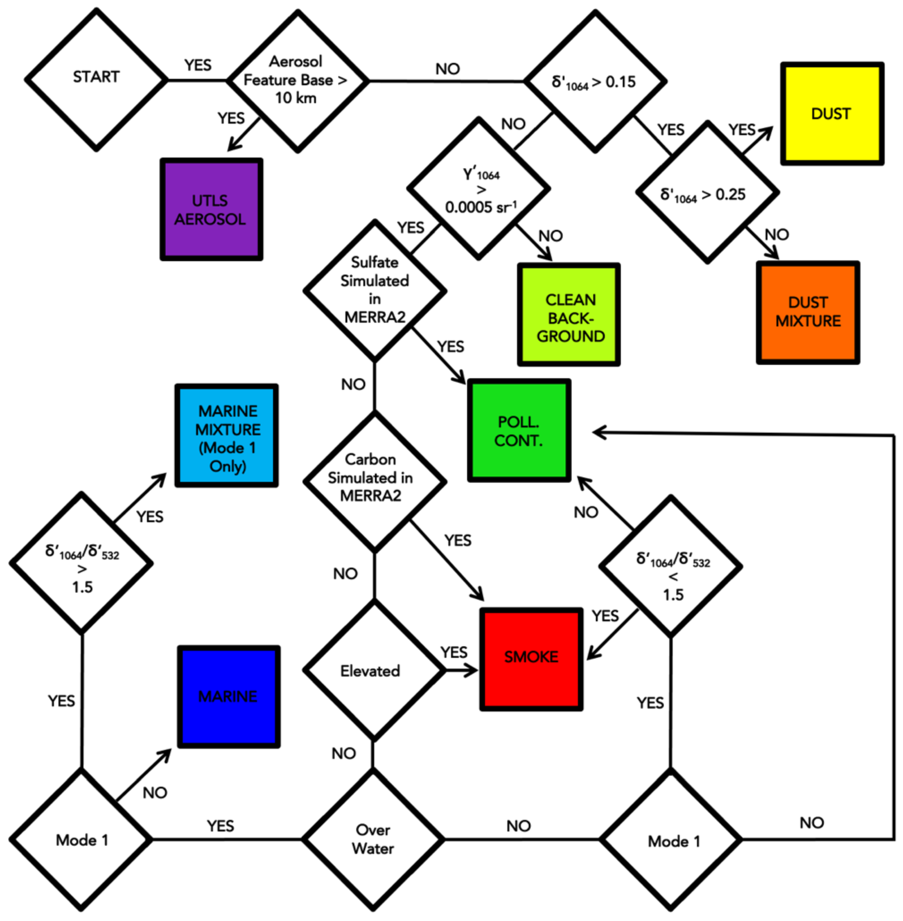
Abstract
:1. Introduction
2. CATS Aerosol-Typing Algorithm Description
3. ISS Orbit Implications for Sampling of Diurnal Variability of Aerosol Vertical Distributions
4. Summary and Conclusions
Supplementary Materials
Author Contributions
Funding
Institutional Review Board Statement
Informed Consent Statement
Data Availability Statement
Acknowledgments
Conflicts of Interest
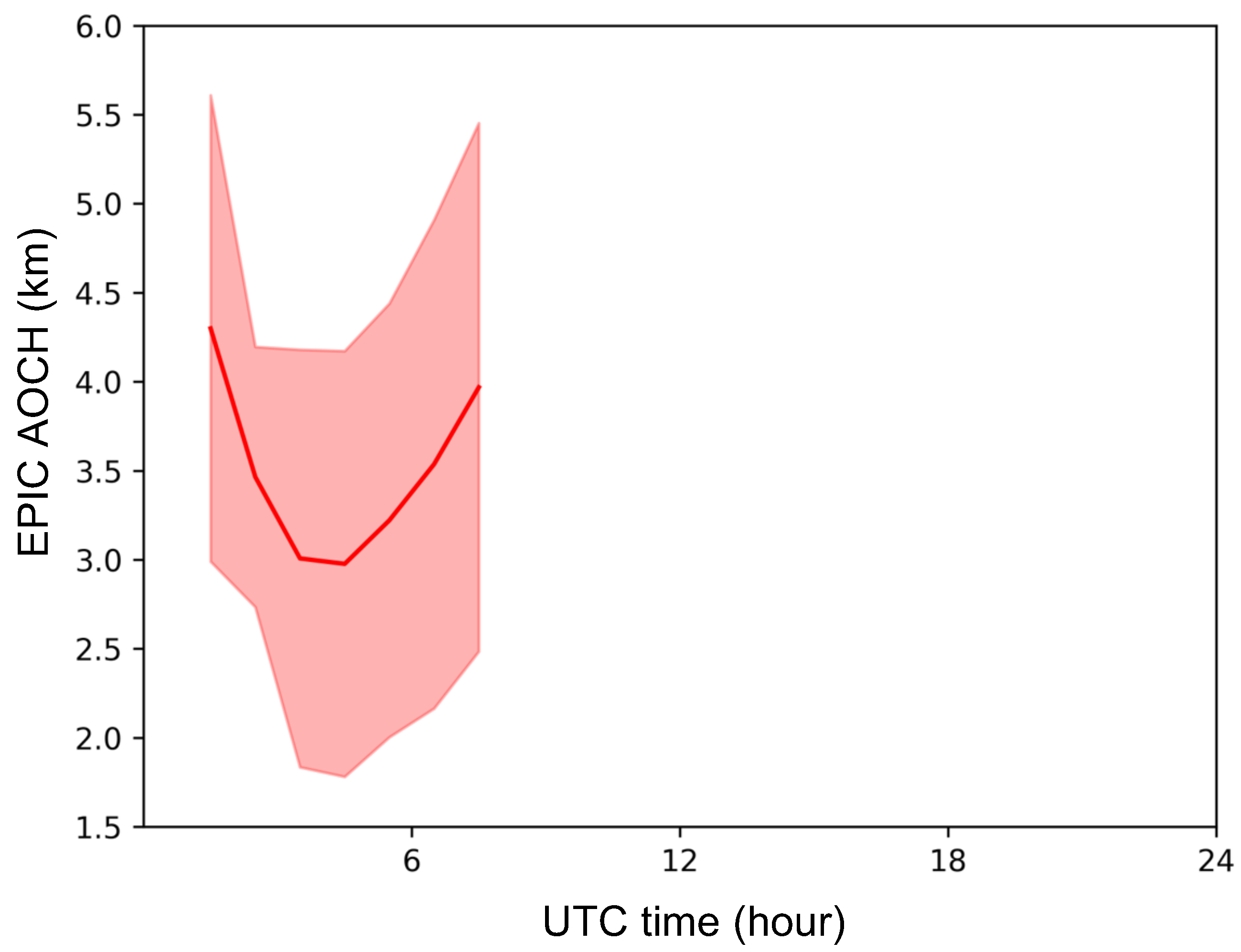
Appendix A. EPIC Aerosol Analysis

References
- Zarzycki, C.M.; Bond, T.C. How much can the vertical distribution of black carbon affect its global direct radiative forcing? Geophys. Res. Lett. 2010, 37. [Google Scholar] [CrossRef]
- Boucher, O.; Randall, D.; Artaxo, P.; Bretherton, C.; Feingold, G.; Forster, P.; Kerminen, V.M.; Kondo, Y.; Liao, H.; Lohmann, U.; et al. Clouds and Aerosols. In Climate Change 2013: The Physical Science Basis. Contribution of Working Group I to the Fifth Assessment Report of the Intergovernmental Panel on Climate Change; Cambridge University Press: Cambridge, UK, 2013; pp. 571–657. [Google Scholar]
- Crutzen, P.J.; Andreae, M.O. Biomass Burning in the Tropics: Impact on Atmospheric Chemistry and Biogeochemical Cycles. Science 1990, 250, 1669–1678. [Google Scholar] [CrossRef]
- Ackerman, A.S.; Toon, O.B.; Stevens, D.E.; Heymsfield, A.J.; Ramanathan, V.; Welton, E.J. Reduction of Tropical Cloudiness by Soot. Science 2000, 288, 1042–1047. [Google Scholar] [CrossRef] [PubMed]
- Samset, B.H.; Myhre, G. Vertical dependence of black carbon, sulphate and biomass burning aerosol radiative forcing. Geophys. Res. Lett. 2011, 38. [Google Scholar] [CrossRef]
- Zhang, L.; Li, Q.B.; Gu, Y.; Liou, K.N.; Meland, B. Dust vertical profile impact on global radiative forcing estimation using a coupled chemical-transport–radiative-transfer model. Atmos. Chem. Phys. 2013, 13, 7097–7114. [Google Scholar] [CrossRef]
- Ge, C.; Wang, J.; Reid, J.S. Mesoscale modeling of smoke transport over the Southeast Asian Maritime Continent: Coupling of smoke direct radiative effect below and above the low-level clouds. Atmos. Chem. Phys. 2014, 14, 159–174. [Google Scholar] [CrossRef]
- Goodkind, A.L.; Tessum, C.W.; Coggins, J.S.; Hill, J.D.; Marshall, J.D. Fine-scale damage estimates of particulate matter air pollution reveal opportunities for location-specific mitigation of emissions. Proc. Natl. Acad. Sci. USA 2019, 116, 8775–8780. [Google Scholar] [CrossRef]
- Winker, D.M.; Vaughan, M.A.; Omar, A.; Hu, Y.; Powell, K.A.; Liu, Z.; Hunt, W.H.; Young, S.A. Overview of the CALIPSO Mission and CALIOP Data Processing Algorithms. J. Atmos. Ocean. Technol. 2009, 26, 2310–2323. [Google Scholar] [CrossRef]
- McGill, M.J.; Yorks, J.E.; Scott, V.S.; Kupchock, A.W.; Selmer, P.A. The Cloud-Aerosol Transport System (CATS): A technology demonstration on the International Space Station. In Proceedings of the Lidar Remote Sensing for Environmental Monitoring XV, San Diego, CA, USA, 9–13 August 2015; Volume 9612, p. 96120A. [Google Scholar] [CrossRef]
- Yorks, J.E.; McGill, M.J.; Palm, S.P.; Hlavka, D.L.; Selmer, P.A.; Nowottnick, E.P.; Vaughan, M.A.; Rodier, S.D.; Hart, W.D. An overview of the CATS level 1 processing algorithms and data products. Geophys. Res. Lett. 2016, 43, 4632–4639. [Google Scholar] [CrossRef] [Green Version]
- Noel, V.; Chepfer, H.; Chiriaco, M.; Yorks, J. The diurnal cycle of cloud profiles over land and ocean between 51° S and 51° N, seen by the CATS spaceborne lidar from the International Space Station. Atmos. Chem. Phys. 2018, 18, 9457–9473. [Google Scholar] [CrossRef]
- Lee, L.; Zhang, J.; Reid, J.S.; Yorks, J.E. Investigation of CATS aerosol products and application toward global diurnal variation of aerosols. Atmos. Chem. Phys. 2019, 19, 12687–12707. [Google Scholar] [CrossRef]
- Knippertz, P.; Todd, M.C. Mineral dust aerosols over the Sahara: Meteorological controls on emission and transport and implications for modeling. Rev. Geophys. 2012, 50. [Google Scholar] [CrossRef]
- Hyer, E.J.; Reid, J.S.; Prins, E.M.; Hoffman, J.P.; Schmidt, C.C.; Miettinen, J.I.; Giglio, L. Patterns of fire activity over Indonesia and Malaysia from polar and geostationary satellite observations. Atmos. Res. 2013, 122, 504–519. [Google Scholar] [CrossRef]
- Kaufman, Y.J.; Ichoku, C.; Giglio, L.; Korontzi, S.; Chu, D.A.; Hao, W.M.; Li, R.R.; Justice, C.O. Fire and smoke observed from the Earth Observing System MODIS instrument–products, validation, and operational use. Int. J. Remote Sens. 2003, 24, 1765–1781. [Google Scholar] [CrossRef]
- Wang, J.; Christopher, S.A.; Nair, U.S.; Reid, J.S.; Prins, E.M.; Szykman, J.; Hand, J.L. Mesoscale modeling of Central American smoke transport to the United States: 1. “Top-down” assessment of emission strength and diurnal variation impacts. J. Geophys. Res. Atmos. 2006, 111. [Google Scholar] [CrossRef]
- Heinold, B.; Knippertz, P.; Marsham, J.H.; Fiedler, S.; Dixon, N.S.; Schepanski, K.; Laurent, B.; Tegen, I. The role of deep convection and nocturnal low-level jets for dust emission in summertime West Africa: Estimates from convection-permitting simulations. J. Geophys. Res. Atmos. 2013, 118, 4385–4400. [Google Scholar] [CrossRef]
- Zhang, J.; Zuidema, P. The diurnal cycle of the smoky marine boundary layer observed during August in the remote southeast Atlantic. Atmos. Chem. Phys. 2019, 19, 14493–14516. [Google Scholar] [CrossRef]
- Hodzic, A.; Duvel, J.P. Impact of Biomass Burning Aerosols on the Diurnal Cycle of Convective Clouds and Precipitation Over a Tropical Island. J. Geophys. Res. Atmos. 2018, 123, 1017–1036. [Google Scholar] [CrossRef]
- Li, Z.; Guo, J.; Ding, A.; Liao, H.; Liu, J.; Sun, Y.; Wang, T.; Xue, H.; Zhang, H.; Zhu, B. Aerosol and boundary-layer interactions and impact on air quality. Natl. Sci. Rev. 2017, 4, 810–833. [Google Scholar] [CrossRef]
- Welton, E.J.; Campbell, J.R.; Spinhirne, J.D.; Scott, V.S. Global monitoring of clouds and aerosols using a network of micropulse lidar systems. Lidar Remote Sens. Ind. Environ. Monit. 2001, 4153, 151–158. [Google Scholar] [CrossRef]
- Yorks, J.E.; Selmer, P.A.; Kupchock, A.; Nowottnick, E.P.; Christian, K.E.; Rusinek, D.; Dacic, N.; McGill, M.J. Aerosol and Cloud Detection Using Machine Learning Algorithms and Space-Based Lidar Data. Atmosphere 2021, 12, 606. [Google Scholar] [CrossRef]
- Omar, A.H.; Winker, D.M.; Vaughan, M.A.; Hu, Y.; Trepte, C.R.; Ferrare, R.A.; Lee, K.P.; Hostetler, C.A.; Kittaka, C.; Rogers, R.R.; et al. The CALIPSO Automated Aerosol Classification and Lidar Ratio Selection Algorithm. J. Atmos. Ocean. Technol. 2009, 26, 1994–2014. [Google Scholar] [CrossRef]
- Loveland, T.R.; Reed, B.C.; Brown, J.F.; Ohlen, D.O.; Zhu, Z.; Yang, L.; Merchant, J.W. Development of a global land cover characteristics database and IGBP DISCover from 1 km AVHRR data. Int. J. Remote Sens. 2000, 21, 1303–1330. [Google Scholar] [CrossRef]
- Nowottnick, E.; Colarco, P.; da Silva, A.; Hlavka, D.; McGill, M. The fate of saharan dust across the atlantic and implications for a central american dust barrier. Atmos. Chem. Phys. 2011, 11, 8415–8431. [Google Scholar] [CrossRef]
- Braun, S.A.; Newman, P.A.; Heymsfield, G.M. NASA’s Hurricane and Severe Storm Sentinel (HS3) Investigation. Bull. Am. Meteorol. Soc. 2016, 97, 2085–2102. [Google Scholar] [CrossRef]
- Nowottnick, E.P.; Colarco, P.R.; Welton, E.J.; da Silva, A. Use of the CALIOP vertical feature mask for evaluating global aerosol models. Atmos. Meas. Tech. 2015, 8, 3647–3669. [Google Scholar] [CrossRef]
- Burton, S.P.; Vaughan, M.A.; Ferrare, R.A.; Hostetler, C.A. Separating mixtures of aerosol types in airborne High Spectral Resolution Lidar data. Atmos. Meas. Tech. 2014, 7, 419–436. [Google Scholar] [CrossRef]
- Burton, S.P.; Ferrare, R.A.; Hostetler, C.A.; Hair, J.W.; Rogers, R.R.; Obland, M.D.; Butler, C.F.; Cook, A.L.; Harper, D.B.; Froyd, K.D. Aerosol classification using airborne High Spectral Resolution Lidar measurements—Methodology and examples. Atmos. Meas. Tech. 2012, 5, 73–98. [Google Scholar] [CrossRef]
- Kim, M.H.; Omar, A.H.; Tackett, J.L.; Vaughan, M.A.; Winker, D.M.; Trepte, C.R.; Hu, Y.; Liu, Z.; Poole, L.R.; Pitts, M.C.; et al. The CALIPSO version 4 automated aerosol classification and lidar ratio selection algorithm. Atmos. Meas. Tech. 2018, 11, 6107–6135. [Google Scholar] [CrossRef] [Green Version]
- Gelaro, R.; McCarty, W.; Suárez, M.J.; Todling, R.; Molod, A.; Takacs, L.; Randles, C.A.; Darmenov, A.; Bosilovich, M.G.; Reichle, R.; et al. The Modern-Era Retrospective Analysis for Research and Applications, Version 2 (MERRA-2). J. Clim. 2017, 30, 5419–5454. [Google Scholar] [CrossRef]
- Randles, C.A.; Silva, A.M.d.; Buchard, V.; Colarco, P.R.; Darmenov, A.; Govindaraju, R.; Smirnov, A.; Holben, B.; Ferrare, R.; Hair, J.; et al. The MERRA-2 Aerosol Reanalysis, 1980 Onward. Part I: System Description and Data Assimilation Evaluation. J. Clim. 2017, 30, 6823–6850. [Google Scholar] [CrossRef] [PubMed]
- Buchard, V.; Randles, C.A.; Silva, A.M.d.; Darmenov, A.; Colarco, P.R.; Govindaraju, R.; Ferrare, R.; Hair, J.; Beyersdorf, A.J.; Ziemba, L.D.; et al. The MERRA-2 Aerosol Reanalysis, 1980 Onward. Part II: Evaluation and Case Studies. J. Clim. 2017, 30, 6851–6872. [Google Scholar] [CrossRef] [PubMed]
- Chin, M.; Ginoux, P.; Kinne, S.; Torres, O.; Holben, B.N.; Duncan, B.N.; Martin, R.V.; Logan, J.A.; Higurashi, A.; Nakajima, T. Tropospheric Aerosol Optical Thickness from the GOCART Model and Comparisons with Satellite and Sun Photometer Measurements. J. Atmos. Sci. 2002, 59, 461–483. [Google Scholar] [CrossRef]
- Colarco, P.; Silva, A.d.; Chin, M.; Diehl, T. Online simulations of global aerosol distributions in the NASA GEOS-4 model and comparisons to satellite and ground-based aerosol optical depth. J. Geophys. Res. Atmos. 2010, 115. [Google Scholar] [CrossRef]
- Darmenov, A.S.; da Silva, A. The Quick Fire Emissions Dataset (QFED): Documentation of versions 2.1, 2.2 and 2.4. In Technical Report Series on Global Modeling and Data Assimilation; National Aeronautics and Space Administration: Washington, DC, USA, 2015; Volume 38, p. 212. [Google Scholar]
- Hess, M.; Koepke, P.; Schult, I. Optical Properties of Aerosols and Clouds: The Software Package OPAC. Bull. Am. Meteorol. Soc. 1998, 79, 831–844. [Google Scholar] [CrossRef]
- Colarco, P.R.; Nowottnick, E.P.; Randles, C.A.; Yi, B.; Yang, P.; Kim, K.M.; Smith, J.A.; Bardeen, C.G. Impact of radiatively interactive dust aerosols in the NASA GEOS-5 climate model: Sensitivity to dust particle shape and refractive index. J. Geophys. Res. Atmos. 2014, 119, 753–786. [Google Scholar] [CrossRef]
- Remer, L.A.; Kaufman, Y.J.; Tanré, D.; Mattoo, S.; Chu, D.A.; Martins, J.V.; Li, R.R.; Ichoku, C.; Levy, R.C.; Kleidman, R.G.; et al. The MODIS Aerosol Algorithm, Products, and Validation. J. Atmos. Sci. 2005, 62, 947–973. [Google Scholar] [CrossRef]
- Levy, R.C.; Remer, L.A.; Kleidman, R.G.; Mattoo, S.; Ichoku, C.; Kahn, R.; Eck, T.F. Global evaluation of the Collection 5 MODIS dark-target aerosol products over land. Atmos. Chem. Phys. 2010, 10, 10399–10420. [Google Scholar] [CrossRef]
- Heidinger, A.K.; Foster, M.J.; Walther, A.; Zhao, X.T. The Pathfinder Atmospheres–Extended AVHRR Climate Dataset. Bull. Am. Meteorol. Soc. 2014, 95, 909–922. [Google Scholar] [CrossRef]
- Kahn, R.A.; Gaitley, B.J.; Martonchik, J.V.; Diner, D.J.; Crean, K.A.; Holben, B. Multiangle Imaging Spectroradiometer (MISR) global aerosol optical depth validation based on 2 years of coincident Aerosol Robotic Network (AERONET) observations. J. Geophys. Res. Atmos. 2005, 110. [Google Scholar] [CrossRef]
- Holben, B.N.; Eck, T.F.; Slutsker, I.; Tanré, D.; Buis, J.P.; Setzer, A.; Vermote, E.; Reagan, J.A.; Kaufman, Y.J.; Nakajima, T.; et al. AERONET—A Federated Instrument Network and Data Archive for Aerosol Characterization. Remote Sens. Environ. 1998, 66, 1–16. [Google Scholar] [CrossRef]
- Hsu, N.C.; Lee, J.; Sayer, A.M.; Kim, W.; Bettenhausen, C.; Tsay, S.C. VIIRS Deep Blue Aerosol Products Over Land: Extending the EOS Long-Term Aerosol Data Records. J. Geophys. Res. Atmos. 2019, 124, 4026–4053. [Google Scholar] [CrossRef]
- Chiapello, I.; Moulin, C. TOMS and METEOSAT satellite records of the variability of Saharan dust transport over the Atlantic during the last two decades (1979–1997). Geophys. Res. Lett. 2002, 29, 17-1–17-4. [Google Scholar] [CrossRef]
- Karyampudi, V.M.; Palm, S.P.; Reagen, J.A.; Fang, H.; Grant, W.B.; Hoff, R.M.; Moulin, C.; Pierce, H.F.; Torres, O.; Browell, E.V.; et al. Validation of the Saharan Dust Plume Conceptual Model Using Lidar, Meteosat, and ECMWF Data. Bull. Am. Meteorol. Soc. 1999, 80, 1045–1076. [Google Scholar] [CrossRef]
- Carlson, T.N.; Prospero, J.M. The Large-Scale Movement of Saharan Air Outbreaks over the Northern Equatorial Atlantic. J. Appl. Meteorol. Climatol. 1972, 11, 283–297. [Google Scholar] [CrossRef]
- Christian, K.; Wang, J.; Ge, C.; Peterson, D.; Hyer, E.; Yorks, J.; McGill, M. Radiative Forcing and Stratospheric Warming of Pyrocumulonimbus Smoke Aerosols: First Modeling Results With Multisensor (EPIC, CALIPSO, and CATS) Views from Space. Geophys. Res. Lett. 2019, 46, 10061–10071. [Google Scholar] [CrossRef]
- Peterson, D.A.; Hyer, E.J.; Campbell, J.R.; Fromm, M.D.; Hair, J.W.; Butler, C.F.; Fenn, M.A. The 2013 Rim Fire: Implications for Predicting Extreme Fire Spread, Pyroconvection, and Smoke Emissions. Bull. Am. Meteorol. Soc. 2015, 96, 229–247. [Google Scholar] [CrossRef]
- Gonzalez-Alonso, L.; Val Martin, M.; Kahn, R.A. Biomass-burning smoke heights over the Amazon observed from space. Atmos. Chem. Phys. 2019, 19, 1685–1702. [Google Scholar] [CrossRef]
- Holben, B.N.; Setzer, A.; Eck, T.F.; Pereira, A.; Slutsker, I. Effect of dry-season biomass burning on Amazon basin aerosol concentrations and optical properties, 1992–1994. J. Geophys. Res. Atmos. 1996, 101, 19465–19481. [Google Scholar] [CrossRef]
- Eck, T.F.; Holben, B.N.; Reid, J.S.; Mukelabai, M.M.; Piketh, S.J.; Torres, O.; Jethva, H.T.; Hyer, E.J.; Ward, D.E.; Dubovik, O.; et al. A seasonal trend of single scattering albedo in southern African biomass-burning particles: Implications for satellite products and estimates of emissions for the world’s largest biomass-burning source. J. Geophys. Res. Atmos. 2013, 118, 6414–6432. [Google Scholar] [CrossRef]
- Herman, J.R.; Bhartia, P.K.; Torres, O.; Hsu, C.; Seftor, C.; Celarier, E. Global distribution of UV-absorbing aerosols from Nimbus 7/TOMS data. J. Geophys. Res. Atmos. 1997, 102, 16911–16922. [Google Scholar] [CrossRef]
- Di Pierro, M.; Jaeglé, L.; Anderson, T.L. Satellite observations of aerosol transport from East Asia to the Arctic: Three case studies. Atmos. Chem. Phys. 2011, 11, 2225–2243. [Google Scholar] [CrossRef]
- Yu, H.; Remer, L.A.; Chin, M.; Bian, H.; Kleidman, R.G.; Diehl, T. A satellite-based assessment of transpacific transport of pollution aerosol. J. Geophys. Res. Atmos. 2008, 113. [Google Scholar] [CrossRef]
- Campbell, J.R.; Ge, C.; Wang, J.; Welton, E.J.; Bucholtz, A.; Hyer, E.J.; Reid, E.A.; Chew, B.N.; Liew, S.C.; Salinas, S.V.; et al. Applying Advanced Ground-Based Remote Sensing in the Southeast Asian Maritime Continent to Characterize Regional Proficiencies in Smoke Transport Modeling. J. Appl. Meteorol. Climatol. 2016, 55, 3–22. [Google Scholar] [CrossRef]
- Welton, E.J.; Stewart, S.A.; Lewis, J.R.; Belcher, L.R.; Campbell, J.R.; Lolli, S. Status of the NASA Micro Pulse Lidar Network (MPLNET): Overview of the network and future plans, new version 3 data products, and the polarized MPL. EPJ Web Conf. 2018, 176, 09003. [Google Scholar] [CrossRef]
- Welton, E.J.; Voss, K.J.; Gordon, H.R.; Maring, H.; Smirnov, A.; Holben, B.; Schmid, B.; Livingston, J.M.; Durkee, P.A.; Formenti, P.; et al. Ground-based lidar measurements of aerosols during ACE-2: Instrument description, results, and comparisons with other ground-based and airborne measurements. Tellus Chem. Phys. Meteorol. 2000, 52, 636–651. [Google Scholar] [CrossRef]
- Welton, E.J.; Voss, K.J.; Quinn, P.K.; Flatau, P.J.; Markowicz, K.; Campbell, J.R.; Spinhirne, J.D.; Gordon, H.R.; Johnson, J.E. Measurements of aerosol vertical profiles and optical properties during INDOEX 1999 using micropulse lidars. J. Geophys. Res. Atmos. 2002, 107, INX2 18-1–INX2 18-20. [Google Scholar] [CrossRef]
- Liu, Z.; Kar, J.; Zeng, S.; Tackett, J.; Vaughan, M.; Avery, M.; Pelon, J.; Getzewich, B.; Lee, K.P.; Magill, B.; et al. Discriminating between clouds and aerosols in the CALIOP version 4.1 data products. Atmos. Meas. Tech. 2019, 12, 703–734. [Google Scholar] [CrossRef]
- Koffi, B.; Schulz, M.; Bréon, F.M.; Griesfeller, J.; Winker, D.; Balkanski, Y.; Bauer, S.; Berntsen, T.; Chin, M.; Collins, W.D.; et al. Application of the CALIOP layer product to evaluate the vertical distribution of aerosols estimated by global models: AeroCom phase I results. J. Geophys. Res. Atmos. 2012, 117. [Google Scholar] [CrossRef] [Green Version]
- Xu, X.; Wang, J.; Wang, Y.; Zeng, J.; Torres, O.; Yang, Y.; Marshak, A.; Reid, J.; Miller, S. Passive remote sensing of altitude and optical depth of dust plumes using the oxygen A and B bands: First results from EPIC/DSCOVR at Lagrange-1 point. Geophys. Res. Lett. 2017, 44, 7544–7554. [Google Scholar] [CrossRef]
- Xu, X.; Wang, J.; Wang, Y.; Zeng, J.; Torres, O.; Reid, J.S.; Miller, S.D.; Martins, J.V.; Remer, L.A. Detecting layer height of smoke aerosols over vegetated land and water surfaces via oxygen absorption bands: Hourly results from EPIC/DSCOVR in deep space. Atmos. Meas. Tech. 2019, 12, 3269–3288. [Google Scholar] [CrossRef]
- Giglio, L. Characterization of the tropical diurnal fire cycle using VIRS and MODIS observations. Remote Sens. Environ. 2007, 108, 407–421. [Google Scholar] [CrossRef]
- Beall, H. Diurnal and seasonal fluctuation of fire-hazard in pine forests. For. Chron. 1934, 10, 209–225. [Google Scholar] [CrossRef]
- Jaffe, D.A.; O’Neill, S.M.; Larkin, N.K.; Holder, A.L.; Peterson, D.L.; Halofsky, J.E.; Rappold, A.G. Wildfire and prescribed burning impacts on air quality in the United States. J. Air Waste Manag. Assoc. 2020, 70, 583–615. [Google Scholar] [CrossRef]
- Lu, Z.; Wang, J.; Xu, X.; Chen, X.; Kondragunta, S.; Torres, O.; Wilcox, E.M.; Zeng, J. Hourly Mapping of the Layer Height of Thick Smoke Plumes over the Western U.S. in 2020 Severe Fire Season. Front. Remote Sens. 2021, 2, 766628. [Google Scholar] [CrossRef]
- Chen, X.; Wang, J.; Xu, X.; Zhou, M.; Zhang, H.; Castro Garcia, L.; Colarco, P.R.; Janz, S.J.; Yorks, J.; McGill, M.; et al. First retrieval of absorbing aerosol height over dark target using TROPOMI oxygen B band: Algorithm development and application for surface particulate matter estimates. Remote Sens. Environ. 2021, 265, 112674. [Google Scholar] [CrossRef]
- Levy, R.C.; Mattoo, S.; Munchak, L.A.; Remer, L.A.; Sayer, A.M.; Patadia, F.; Hsu, N.C. The Collection 6 MODIS aerosol products over land and ocean. Atmos. Meas. Tech. 2013, 6, 2989–3034. [Google Scholar] [CrossRef]
- Schaaf, C.B.; Gao, F.; Strahler, A.H.; Lucht, W.; Li, X.; Tsang, T.; Strugnell, N.C.; Zhang, X.; Jin, Y.; Muller, J.P.; et al. First operational BRDF, albedo nadir reflectance products from MODIS. Remote Sens. Environ. 2002, 83, 135–148. [Google Scholar] [CrossRef]
- Tilstra, L.G.; Tuinder, O.N.E.; Wang, P.; Stammes, P. Surface reflectivity climatologies from UV to NIR determined from Earth observations by GOME-2 and SCIAMACHY. J. Geophys. Res. Atmos. 2017, 122, 4084–4111. [Google Scholar] [CrossRef]
- Wang, J.; Xu, X.; Ding, S.; Zeng, J.; Spurr, R.; Liu, X.; Chance, K.; Mishchenko, M. A numerical testbed for remote sensing of aerosols, and its demonstration for evaluating retrieval synergy from a geostationary satellite constellation of GEO-CAPE and GOES-R. J. Quant. Spectrosc. Radiat. Transf. 2014, 146, 510–528. [Google Scholar] [CrossRef] [Green Version]


Publisher’s Note: MDPI stays neutral with regard to jurisdictional claims in published maps and institutional affiliations. |
© 2022 by the authors. Licensee MDPI, Basel, Switzerland. This article is an open access article distributed under the terms and conditions of the Creative Commons Attribution (CC BY) license (https://creativecommons.org/licenses/by/4.0/).
Share and Cite
Nowottnick, E.P.; Christian, K.E.; Yorks, J.E.; McGill, M.J.; Midzak, N.; Selmer, P.A.; Lu, Z.; Wang, J.; Salinas, S.V. Aerosol Detection from the Cloud–Aerosol Transport System on the International Space Station: Algorithm Overview and Implications for Diurnal Sampling. Atmosphere 2022, 13, 1439. https://doi.org/10.3390/atmos13091439
Nowottnick EP, Christian KE, Yorks JE, McGill MJ, Midzak N, Selmer PA, Lu Z, Wang J, Salinas SV. Aerosol Detection from the Cloud–Aerosol Transport System on the International Space Station: Algorithm Overview and Implications for Diurnal Sampling. Atmosphere. 2022; 13(9):1439. https://doi.org/10.3390/atmos13091439
Chicago/Turabian StyleNowottnick, Edward P., Kenneth E. Christian, John E. Yorks, Matthew J. McGill, Natalie Midzak, Patrick A. Selmer, Zhendong Lu, Jun Wang, and Santo V. Salinas. 2022. "Aerosol Detection from the Cloud–Aerosol Transport System on the International Space Station: Algorithm Overview and Implications for Diurnal Sampling" Atmosphere 13, no. 9: 1439. https://doi.org/10.3390/atmos13091439