Spatiotemporal Modes Characteristics and SARIMA Prediction of Total Column Water Vapor over China during 2002–2022 Based on AIRS Dataset

Abstract

The total column water vapor (TCWV) is a relatively active component in the atmosphere and an important detection object of climate change. Exploring the spatiotemporal modes characteristics of TCWV and predicting its changing trends can provide a reference for human beings to deal with climate change and formulate corresponding countermeasures. The TCWV data over China region by using the Atmospheric Infrared Sounder (AIRS) dataset from 2002 to 2022 were obtained. The empirical orthogonal function (EOF) analysis, linear regression, Mann-Kendall (M-K) mutation test, Seasonal Autoregressive Integrated Moving Average (SARIMA) model and other methods were used to discuss the spatiotemporal modes characteristics of TCWV in the China region on the monthly, seasonal, and annual scales and verify the rationality of the forecast of the monthly average trend of TCWV in the next year. The obtained results show that: (1) The annual and seasonal scales spatial distributions of TCWV in China are roughly consistent, with obvious latitudinal distribution characteristics. That is, the TCWV in the low latitude region, especially in the tropical region, is larger, and it gradually decreases with the increase of the latitude. Furthermore, the TCWV in the eastern region is higher than that in the western region at the same latitude; (2) The EOF analysis results show that its first mode can better reflect the typical distribution characteristics of the southeast-northwest positive distribution in China; (3) From 2002 to 2022, the TCWV in China shows an upward trend and the TCWV increases at a rate of 0.0413 kg/m² per year, which may be related to the long-term increase of air temperature in recent years; (4) The inter-monthly variation of TCWV shows a slightly positive skewed ‘bell-shaped’ curve, with the maximum in summer, the minimum in winter and the similar distribution in spring and autumn. As can be seen from the M-K curves of the four seasons, each season has different mutation points; (5) Forecasting the TCWV was done using time series monthly average values from September 2002 to February 2022. SARIMA (3, 1, 3) × (0, 1, 1, 12) was identified as the best model. This model passed the residual normality test and the forecasting evaluation statistics show that MAPE = 2.65%, MSE = 0.3229 and the R2-score = 0.9949. As demonstrated by the results, the SARIMA model is a good model for forecasting TCWV in the China region.

1. Introduction

Atmospheric water vapor is one of the important parameters of surface atmospheric energy exchange, hydrological cycle and climate change [1,2,3]. There are many acronyms for atmospheric water vapor, such as TCWV (Total Column Water Vapor, TCWV), PW (Precipitable Water vapor, PW), TPW (Total Precipitable Water vapor, TPW) and so on. The acronym of TCWV is used in this study. As the main greenhouse gas in the atmosphere, the changes in TCWV have a significant impact on temperature and precipitation, and the TCWV is closely related to surface evaporation, cloud formation and circulation transportation [4,5,6,7]. In addition, the prediction of TCWV is also of great significance in monitoring small scale disastrous weather. Therefore, the study of the temporal and spatial variation characteristics of TCWV and its prediction are of great importance to global climate change, human life, and production.

The amount of water vapor in the atmospheric column, usually comprehensive water vapor or precipitable steam, can be measured by various techniques. Experts and scholars have carried out a lot of research on TCWV by combining the sounding observation data of meteorological stations, reanalysis data and the relevant empirical formulas. Many studies have shown that the TCWV in China has obvious inter-annual and inter-decadal variation characteristics, and the spatial-temporal distribution of TCWV are influenced by various factors such as seasons, topography and temperature. Wang et al. [8] found that water vapor decreases from southeast to northwest, and it has shown a gradual increasing trend in the Third Pole. Gong et al. [9] reported that the seasonal variation of water vapor content in Northwest China appears to be lowest in winter, followed by spring, then by autumn, and it is the highest in summer. Lu et al. [10] concluded that the first and second EOF modes of tropical Cold Point Tropopause (CPT) variations are related to typical El Niño-Southern (ENSO) activity and sea surface temperature (SST) changes in the central Pacific, respectively. Li et al. [11] applied the Mann–Kendall trend test to analyze the spatiotemporal variations of precipitation. The result revealed that the rainfall amount (RA) increased with the increase of light rain in Northwest China and heavy rain in Southeast China. Su et al. [12] studied the characteristics of the summer atmospheric water cycle in China by using the ERA-Interim and MERRA reanalysis from 1979 to 2012. Wang et al. [13] evaluated the temporal and spatial distribution characteristics of precipitable water (PW) in China, and it showed an overall downward spatial trend from the southeast to the northwest direction, and it was also found that PW was most closely related to precipitation in the northeastern region and the upper northwestern region. Zhao et al. [14] evaluated that the capture capabilities of two satellite data sets (version 6 of AIRS-only and AIRS/AMSU) and seven existing reanalysis datasets (MERRA, MERRA2, NCEP1, NCEP2, CFSR, JRA55, ERA-Interim) for the annual mean climatology, annual cycle and inter-annual variability of the TCWV over the Tibetan Plateau.

Predicting the TCWV in all its forms will be a difficult process when global warming has combined with the variability of nature itself. There has been a great deal of previous research on water vapor prediction. Wei et al. [15] examined the Zhengzhou, China region. They used a wavelet and hybrid model of the complementary ensemble empirical mode decomposition, recurrent neural networks and ARIMA models on an annual precipitation sequence. They found that the relative error of the forecasting in 2013–2017 was 14.1%. Hellen W. Kibunja et al. [16] analyzed the precipitation forecast using a SARIMA model in the Mt. Kenya region. The forecasting evaluation statistics show that ME = −0.0053687, MSE = 0.96794, RMSE = 0.98384 and MAE = 0.75197. Valipour et al. [17] had done a comparative study of SARIMA and ARIMA for runoff in United States. The result shows that SARIMA is better fitted and a better forecaster compared to the ARIMA model. These studies have successfully used the ARIMA and SARIMA models to understand the climate parameters and have given better insight into understanding the hydrological regime of the watersheds.

To sum up the above, most of the previous studies focused on the analysis of local areas in China, and there is still a lack of systematic research on the spatiotemporal mode characteristics of TCWV in the whole region of China. China has a vast territory, the terrain is high in the west and low in the east, and the mountains are diverse. Dunya Alraddawi et al. [18] concluded that the Atmospheric Infrared Sounder (AIRS) showed the best agreement with GNSS time series in the quality of different existing satellite Total Column Water Vapour (TCWV) datasets, namely from the Moderate Resolution Imaging Spectroradiometer (MODIS), AIRS and the SCanning Imaging Absorption spectroMeter for Atmospheric CHartographY (SCIAMACHY). These were used in order to understand the spatial-temporal distribution and trend of TCWV in China more comprehensively. In this paper, a variety of methods were used to analyze the spatiotemporal modes characteristics of TCWV over China in detail based on the AIRS remote sensing dataset, and we forecasted the TCWV for the following year using SARIMA model.

2. Data and Method

2.1. Data

NASA’s Aqua satellite is part of the A-Train orbit satellite constellation that is equipped with six different Earth-observing instruments to measure various parameters related to land, ocean, and Earth’s atmosphere and biosphere, with a concentration on water [19]. The Atmospheric Infrared Sounder (AIRS) can conduct high-precision atmospheric detection under sunny and cloudy conditions [20]. At present, the data detected by AIRS includes three versions: V5, V6 and V7 [21]. In this paper, the AIRS Version 6 Level 3 product was used to extract the TCWV, the Temperature of the Atmosphere at the Earth’s Surface (TAS) and the Surface Skin Temperature (SST) measurements from September 2002 to February 2022 over China (15° N~55° N, 70° E~140° E). The product provides the monthly TCWV, TAS and SST retrievals at a 1 deg. (longitude) × 1 deg. (latitude) resolution.

2.2. Research Methods

2.2.1. Empirical Orthogonal Function (EOF) Analysis Method

Empirical Orthogonal Function (EOF) analysis is also known as eigenvector analysis. EOF is a commonly used analysis method to study the spatial and temporal characteristics of meteorological variables [22]. The application of this technique greatly reduces the dimensionality of an original dataset, while preserving the majority of the variations in the original data as much as possible [23]. And the first few orthogonal models can represent the vast majority of the total variances of the original dataset [24]. The principle is to decompose the meteorological variable field with time and space into a linear combination of spatial pattern (V) and time coefficients (T) that are uncorrelated, which can be expressed in the following matrix form:

$$X_{m\times n}=V_{m\times p}{T}_{p\times n}$$

(1)

This method uses a small number of spatially distributed modes to describe the original variable field, and the basic information of the original variable field can be captured. It provides convenience for studying climate variables. The original variable field is given in matrix form:

$$X=\left(\begin{array}{ccc}{x}_{11}& \dots & x_{1n}\\ ⋮& \ddots & ⋮\\ x_{m1}& \cdots & x_{mn}\end{array}\right)i=1,2,...,m;\begin{array}{cc}& \end{array}j=1,2,...,n$$

(2)

where m is the spatial point and n is the length of time series, i.e., the number of samples; $x_{ij}$ represents the $j$-th observed value on the $i$-th spatial point.

2.2.2. Linear Regression

The annual average time series of TCWV is fitted with a linear model to detect its changing trend in time domain.

$$Y=a\times t+b$$

(3)

In above equation, $a$ is the change speed and $b$ is the intercept. In the fitting process, the least square method is used to minimize the root mean square error between the estimated and the observed value [25].

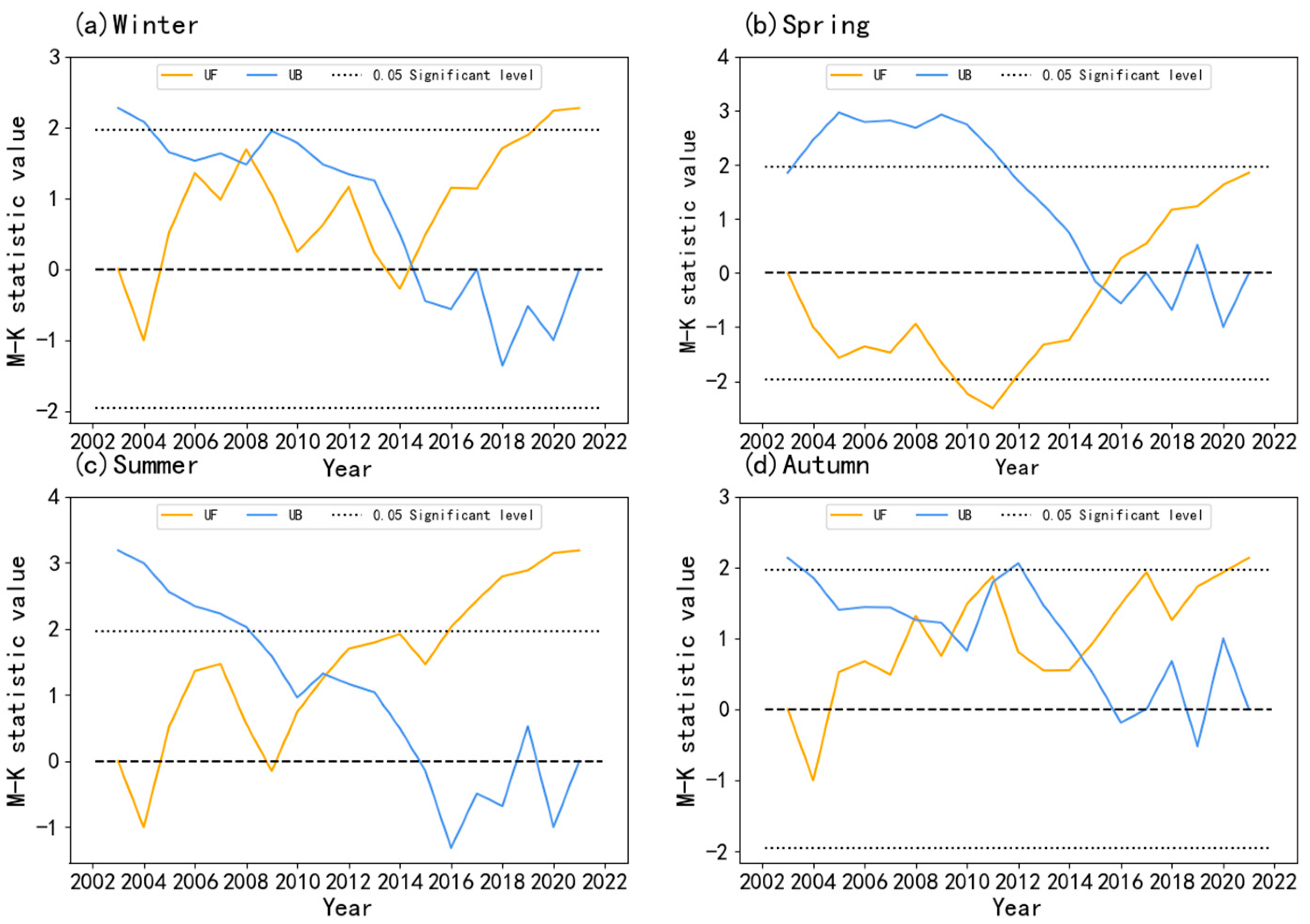
2.2.3. Mann-Kendall Mutation Test

This is a rank nonparametric statistical test that was developed by Mann (1945) and Kendall (1975), and it has advantages in detecting linear or nonlinear trends [26,27]. When the Mann-Kendall (M-K) method can be used to analyze the abrupt change of climate, the sample does not need to obey a certain distribution, and it will not be disturbed by a few abnormal anomalies, so it is more suitable for type variables and sequence variables [28]. It is commonly used in hydrology and meteorology. The general principle of this method is as follows: assuming a time series x with n sample sizes, construct an order sequence:

$$S_k={\displaystyle \sum }_{i=1}^k{r}_i k=2,3, \dots , n$$

(4)

In the above equation (4), $ri$ is expressed as follows:

$$r_i=\{\begin{array}{c} 1, when ( {\displaystyle {\displaystyle \sum }_{j=1}^{i-1}}\mathrm{sgn}(x_i-x_j) ) >0 \\ 0, else\end{array}$$

(5)

Therefore, it can be seen that the rank sequence S_k in Equation (4) is the cumulative number of times the value of i at the moment i is greater than the number of values at time j. Under the assumption of the random independence of a time series, define the statistics:

$$U{F}_k=\frac{S_k-E\left(S_k\right)}{\sqrt{V_{ar}\left(S_k\right)}} k=1,2,3,...,n$$

(6)

$U{F}_1=0$, $E\left(S_k\right)$ and $V_{ar}\left(S_k\right)$ are the expectation and variance of the cumulative $S_k$, respectively [29]. When time series $x_1$, $x_2,$ ……, $x_n$ are independent and identically distributed, $E\left(S_k\right)$ and $V_{ar}\left(S_k\right)$ can be calculated by the following formula:

$$E\left(S_k\right)=\frac{k\left(k-1\right)}{4}$$

(7)

$$V_{ar}\left(S_k\right)=\frac{k\left(k-1\right)\left(2k+5\right)}{72}$$

(8)

$U{F}_k$ converges to the standard normal distribution, which is a statistics sequence by calculated time series x order $x_1$, $x_2$, …, $x_n.$ Given a significant level α, in comparison with the data in the table of known normal distribution, and if $\left|U{F}_k\right|>U_{\alpha }$, then there are significant changes in the trend. In a similar process to UF, the UB values are calculated backwards from the end of the sequence, thus making $U{F}_k=-U{B}_k$.

Given the significance level α, the two curves of $U{F}_k$ and $U{B}_k$ are plotted on the same graph as well as the significant horizontal line. If the value of $U{F}_k$ is greater than 0, there is an upward trend in the sequence; while a value below 0 indicates a downward trend. When the value exceeds the critical line, it indicates that the upward or downward trend is significant, and the range beyond the critical line is defined as the time zone of mutation. If the $U{F}_k$ and $U{B}_k$ curves appear on an intersection point, and the intersection point is between the critical line, then the corresponding time of the intersection point is the beginning time of the mutation; if the intersection point is outside the critical line, or there are multiple obvious intersection points, it is unclear whether it is a mutation point.

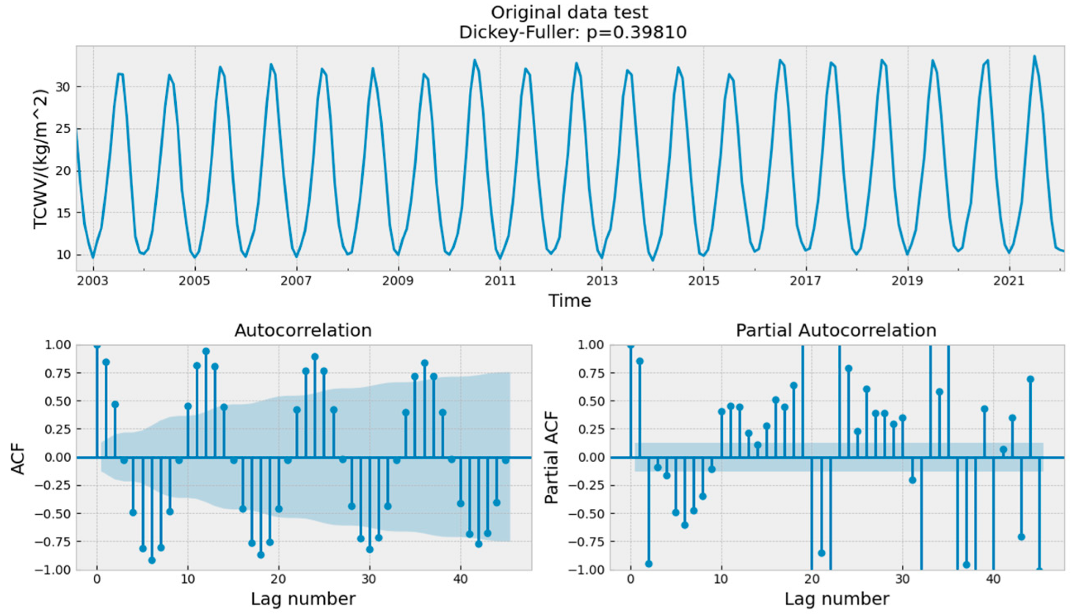
2.2.4. Seasonal Autoregressive Integrated Moving Average (SARIMA) Forecast Analysis

The autoregressive integrated moving average model (ARIMA) may be helpful for time series prediction. It has been proposed by Box and Jenkins in 1976 [30,31]. As an improved form of the ARIMA model, the SARIMA model is used for periodic time series and performs the seasonal difference on the basis of the ARIMA model [32]. The SARIMA model is defined as:

$$\mathrm{SARIMA}=(\mathrm{q}, \mathrm{d}, \mathrm{q})\times {(\mathrm{P}, \mathrm{D}, \mathrm{Q})}_{\mathrm{s}}$$

(9)

where p, d and q are the autoregressive, differencing and moving average orders in the non-seasonal part of the model; the P, D and Q are the values of autoregressive, differencing and moving average orders in the seasonal part of model [33]. These term are determined by an autocorrelation function (ACF) and a partial autocorrelation function (PACF) [34]. Finally the s is the length of seasonality.

The identification of the SARIMA model follows:

(1)

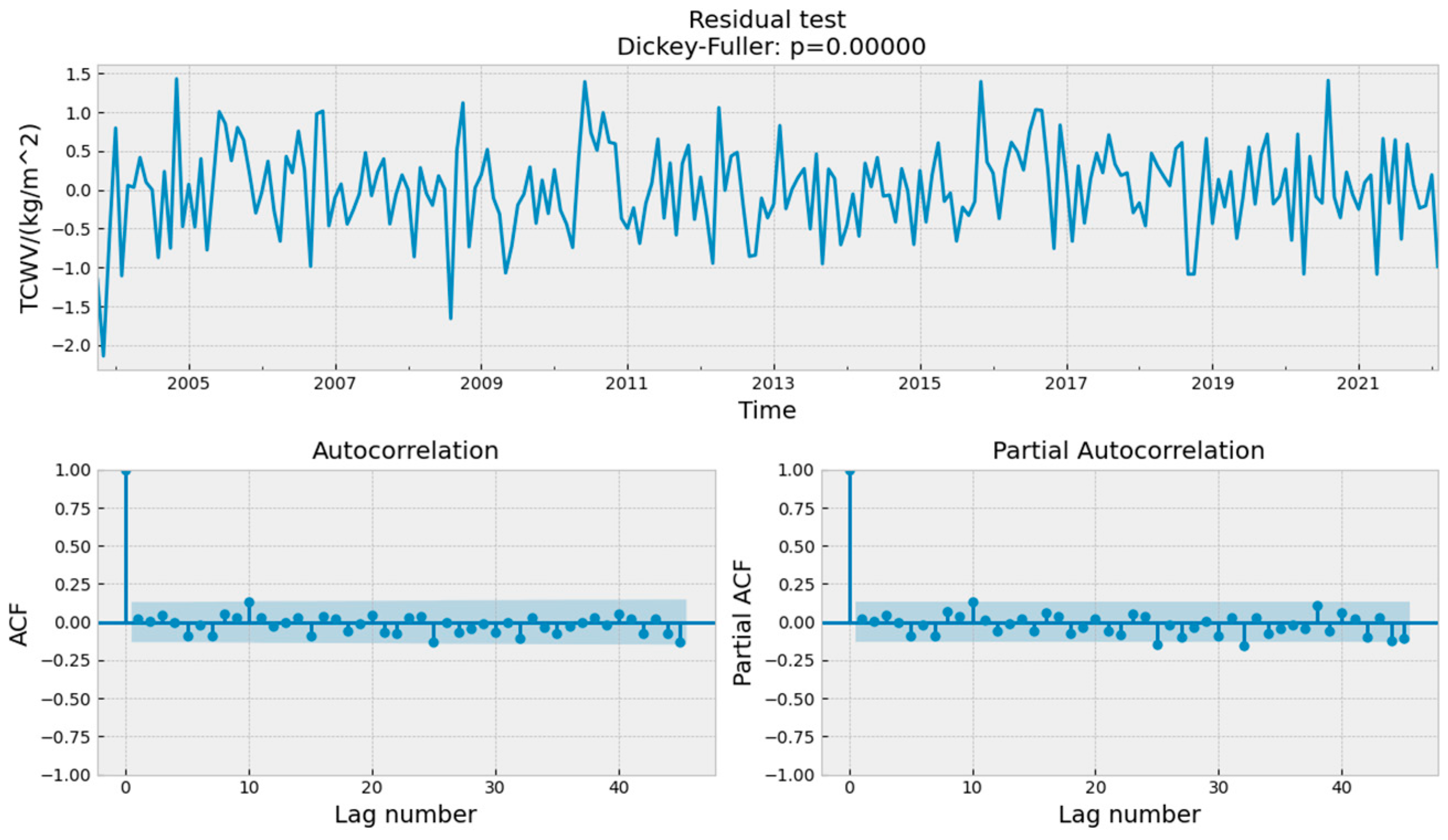
To judge the stationarity of a sequence, this paper uses the Dickey-Fuller (DF) unit root test to judge whether the sequence is stationarity.

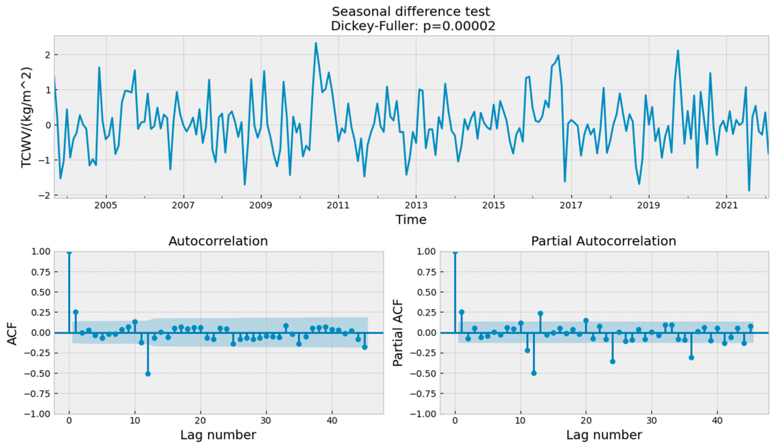
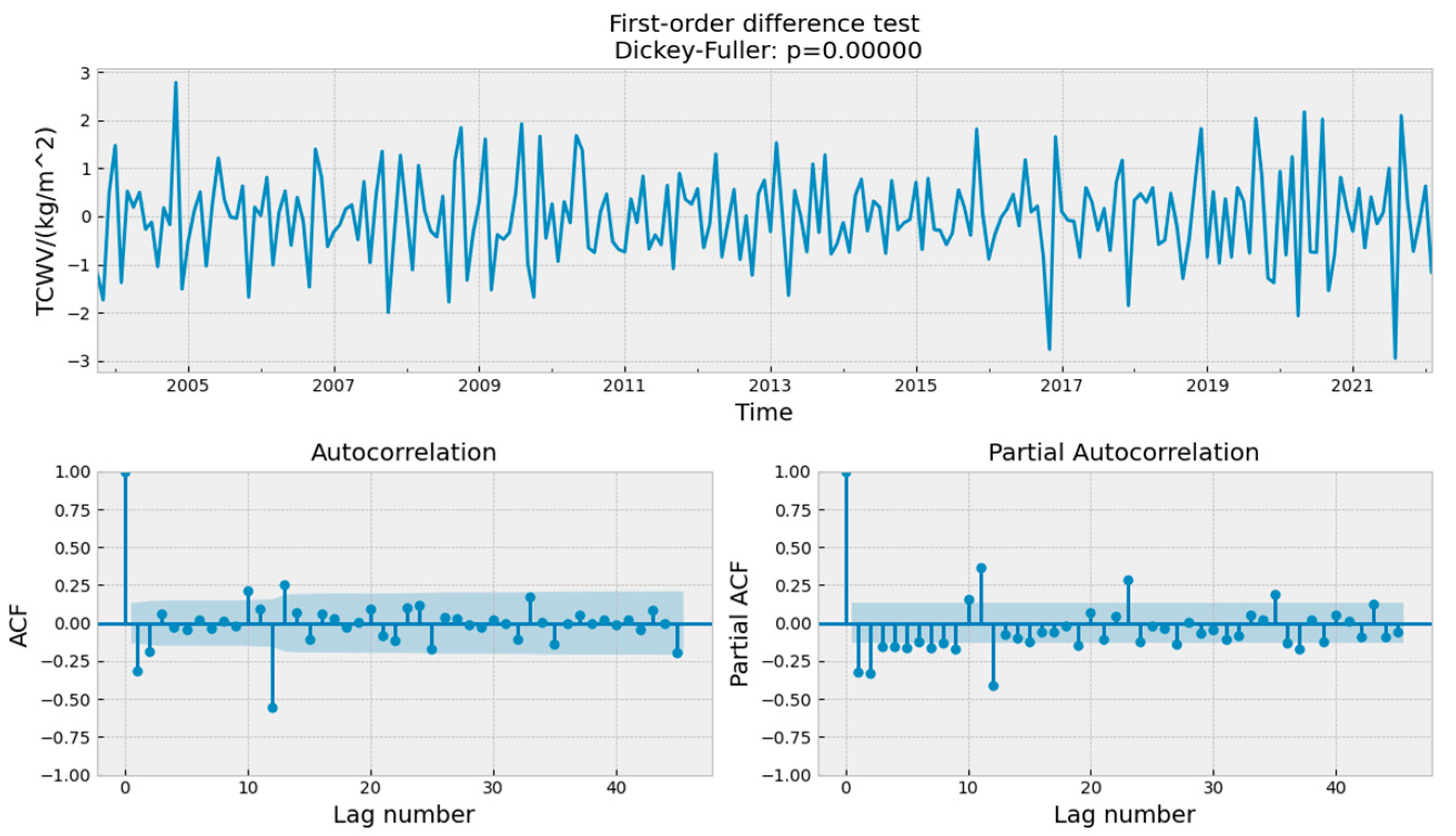
(2)

If the sequence is non stationary, it is processed by difference, eliminating the fluctuation of the sequence to make the data tend to be stationary, and extracting the effective information in the sequence.

(3)

Order the model. In this paper, the autocorrelation, partial correlation and criterion functions are used.

(4)

Test the model, including residual DF unit root test, residual Ljung-Box Q (LBQ) test and residual white noise test. If there are insignificant parameters, it is necessary to eliminate them and readjust the model structure [35,36]. The white noise test ensures that the model can fully extract the relevant information of the sequence.

2.2.5. Pearson Correlation Coefficient

The Pearson correlation coefficient is a linear correlation coefficient used to reflect the linear correlation of two continuous variables. The correlation coefficient of different elements can be calculated through covariance. For any two variables, X and Y, the formula for calculating the Pearson correlation coefficient is given as follows:

$$r=\frac{{\displaystyle \sum }\left(X-\overline{X}\right)\left(Y-\overline{Y}\right)}{\sqrt{\sum {\left(X-\overline{X}\right)}^2}\sqrt{{\displaystyle \sum }{\left(Y-\overline{Y}\right)}^2}}$$

(10)

where $r$ is the correlation coefficient, and $r>0$ is a positive correlation, $r<0$ is a negative correlation; the greater the absolute value of $r$, the stronger the correlation.

3. Results

3.1. Spatial Distribution Characteristics of TCWV in China

3.1.1. Spatial Distribution Characteristics of Annual mean TCWV in China

We selected the data of TCWV in China from September 2002 to February 2022, provided by the AIRS dataset, and calculated the average value of TCWV over the China region during these 20 years. Figure 1a shows the variation trend of TCWV with longitude, showing a “V” shape as a whole. In the regions with longitude ranging from 70° E to 100° E, the TCWV decreases with the increase of longitude; in the regions with longitude ranging from 100° E to 140° E, the TCWV increases with the increase of longitude. The main reason is that the areas of 70° E~100° E is mainly the Tibetan Plateau, which is the Third Pole in the world. Figure 1b shows the variation trend of the TCWV with latitude. It can be seen that the TCWV in China decreases with the increase of latitude. This is mostly related to the temperature, with higher temperatures in lower latitudes, making it easier for moisture to evaporate, thus allowing more water vapor to enter the air. The 20-year average spatial distribution of the TCWV in China is shown in Figure 1c. The 20-year average value of the TCWV over the China region ranges from 2.27 kg/m² to 47.29 kg/m², with the maximum value located in South China and the minimum value located at the junction of southwest and northwest China. It can be seen from Figure 1c that the TCWV in China has an obvious southeast-northwest distribution, that is, the TCWV in the southeast is higher than that in the northwest. This is mainly because the southeastern region is closer to the ocean, while the northwest China region is deep inland and far away from the ocean, making it difficult for the humid air brought by the monsoon from the ocean to reach the region. On the other hand, it is also because most of the northwest region is desert, which is arid and short of water, so therefore less water can enter the air by evaporation. The other special area is the Tibetan Plateau. It can be seen from Figure 1c that the latitude of the Tibetan Plateau is lower than that of northwest China, but the TCWV is also lower, which is obviously related to the altitude of the Tibetan Plateau. On the one hand, high mountains have a certain influence on the transportation of the TCWV; on the other hand, the higher the altitude, the shorter the column of air above the water vapor, and thus the TCWV is lower. Therefore, generally speaking, the distribution of TCWV in China is related to latitude, distance from the ocean, and altitude. These conclusions are consistent with the work of [37].

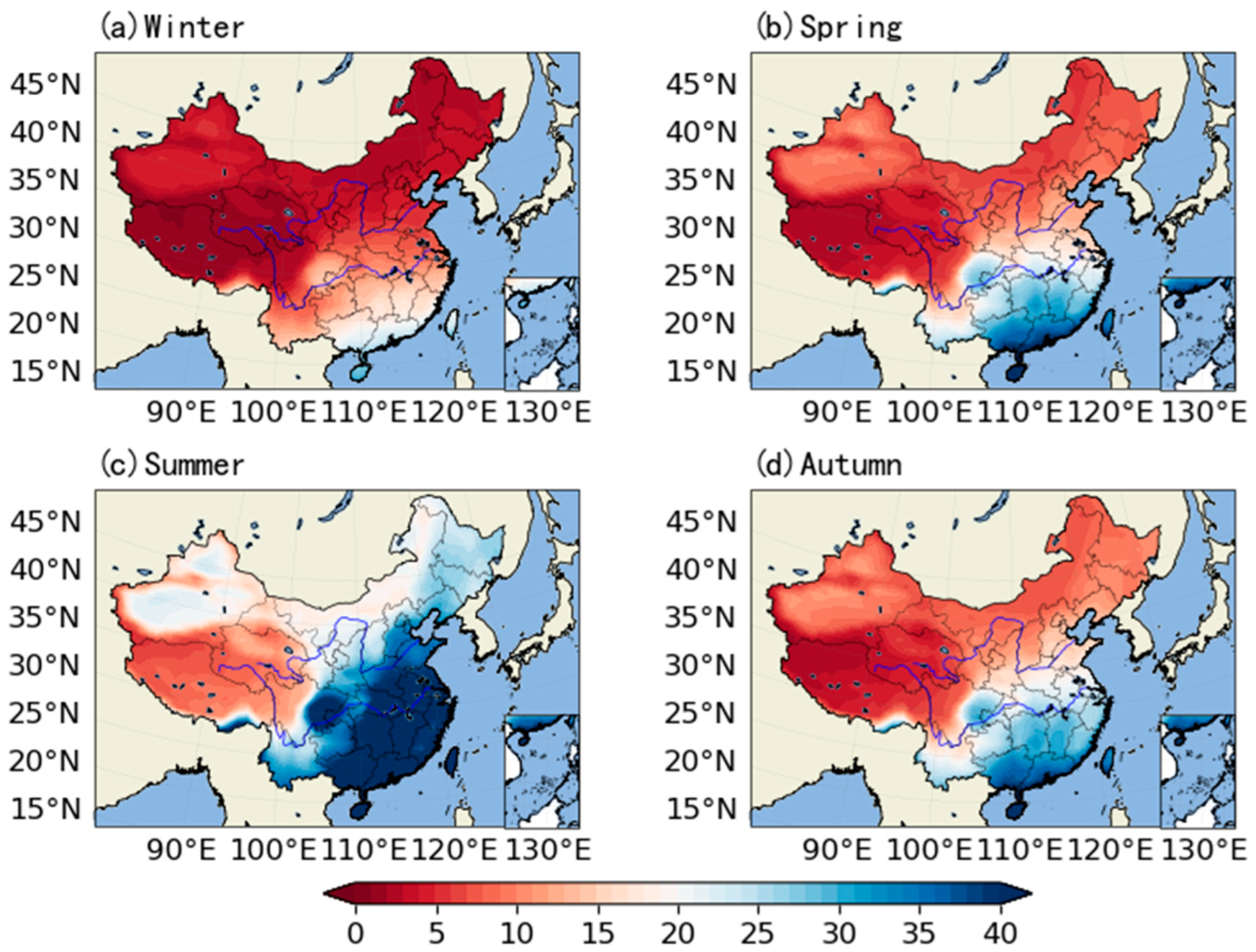
3.1.2. Seasonal Spatial Distribution Characteristics of TCWV

In this paper, the average value of TCWV from March to May is selected to investigate the distribution of TCWV in spring in China. Similarly, June to August, September to November, and December to next February were selected as the seasons of summer, autumn, and winter, respectively. The distribution of the TCWV in each season is shown in Figure 2. It can be seen from Figure 2 that the TCWV is the lowest in winter and the highest in summer, which is more obvious in South, East and Central China. In winter, the coastal provinces of Yunnan, Guangxi, Guangdong, Fujian and Hainan have higher TCWV values due to the influence of tropical ocean water vapor. The TCWV in most other areas is low, and its distribution is higher in low latitudes than in high latitudes, higher in plains than in plateaus, and higher in coastal areas than inland areas. In spring, the TCWV increases in most parts of China, among which the increase is more obvious in southern China and its coastal areas, and is somewhat faster in the central China and the coastal East China than in the same latitude regions. Entering summer, due to the influence of East Asian summer monsoons, the maximum value of TCWV in China is located in the southeast, and the northwest is relatively dry, while the TCWV shows a southwest–northeast trend. Specifically, starting from May, with the establishment and development of the East Asian summer monsoon, the TCWV begins to increase over the southeast of the Tibetan Plateau and southern China in China, and the maximum value of TCWV keeps advancing to the northwest with time; in June, the maximum value of TCWV pushes to the position of 30° N. In autumn, with the weakening of monsoon intensity, the high-value areas of TCWV in China starts to retreat to southward, and the TCWV over southeast China and the Tibetan Plateau gradually decreases. The distribution of TCWV is very similar to that in spring, except for southern China where the TCWV is lower than that in spring, and all other areas are higher than that in spring. Generally speaking, the spatial distribution of TCWV in China is not uniform, with more in southeast China, less in northwest China, more in coastal areas, less in inland areas, more in mountainous areas and less in plain areas. The TCWV in the same area is generally greater in the summer and less in the winter.

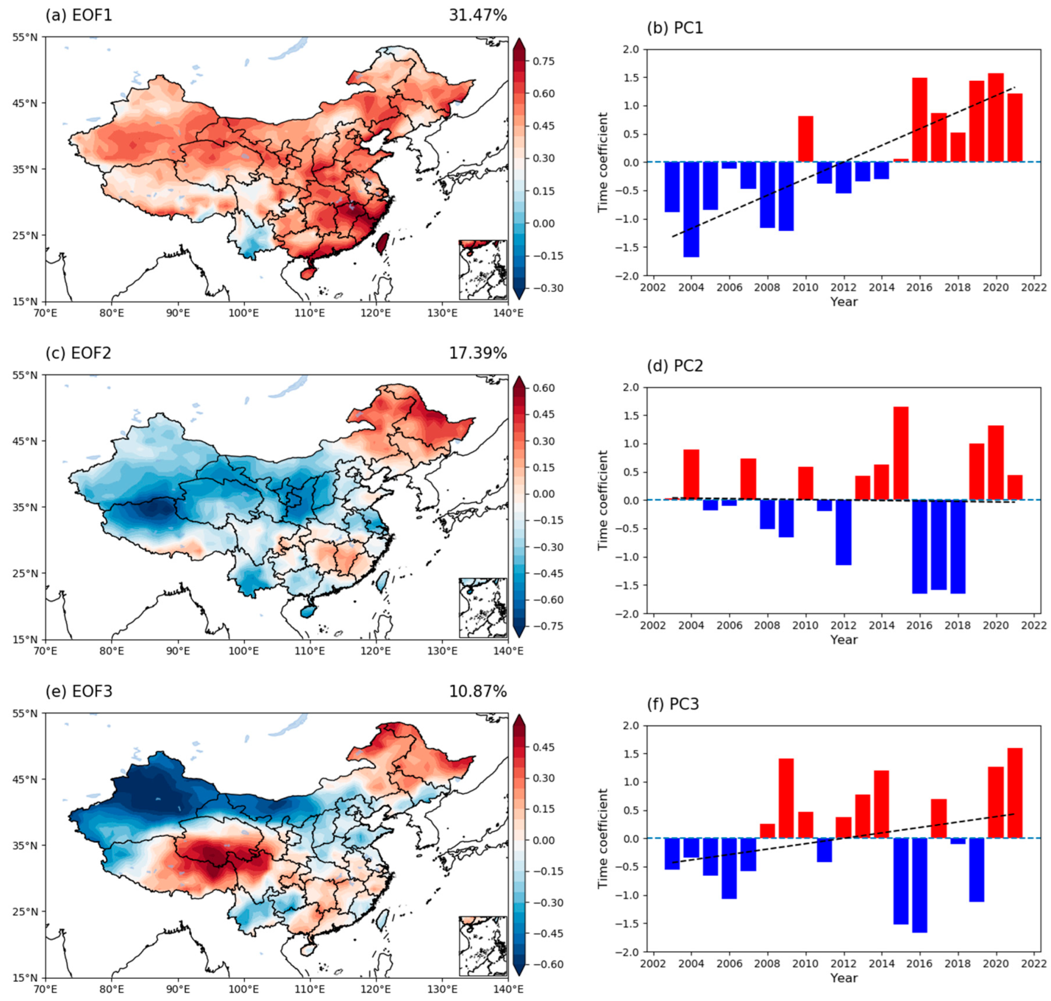
3.1.3. EOF Analysis of TCWV Spatial Distribution in China

To further study the spatiotemporal variations of the TCWV, an EOF analysis was performed on TCWV from the AIRS dataset to identify the dominant modes of year-to-year variation. The spatial distribution of the three leading EOF modes and their corresponding time series are presented in Figure 3. This shows that the cumulative variance contribution rate of the first three modes of EOF analysis of TCWV is 59.73%, that is, the change information of the first three modes representing the original variable field is 59.73%. Therefore, the spatial distribution of the first three eigenvectors can represent the main distribution type of the TCWV throughout the year. The first three modes of EOF were mainly analyzed as follows. Figure 3a shows that the first EOF mode of TCWV variation accounts for 31.47% of the total variance during 2003–2021, indicating that the TCWV has good convergence in space. The TCWV values of the first spatial mode of EOF is positive in most areas except for the southwest border, which is basically the inverse northwest–southeast type. From Figure 3c, the second spatial mode of EOF analysis value of TCWV is low in most areas except for the northeast of China, indicating the consistency of TCWV distribution in China. From Figure 3e, the value of TCWV of the third spatial mode of EOF presents a ‘positive-negative’ pattern from south to north and the maximum on the Tibetan Plateau. In addition, the time coefficient corresponding to the feature vector represents the time variation characteristics of the distribution pattern characterized by the feature vector in the region. The results of the first temporal mode and the third temporal mode of EOF analysis demonstrate that TCWV has shown similar increasing trends over the past 19 years (Figure 3b, f) except for the second temporal mode of the TCWV of EOF (Figure 3d).

3.2. Temporal Variation Characteristics of TCWV in China

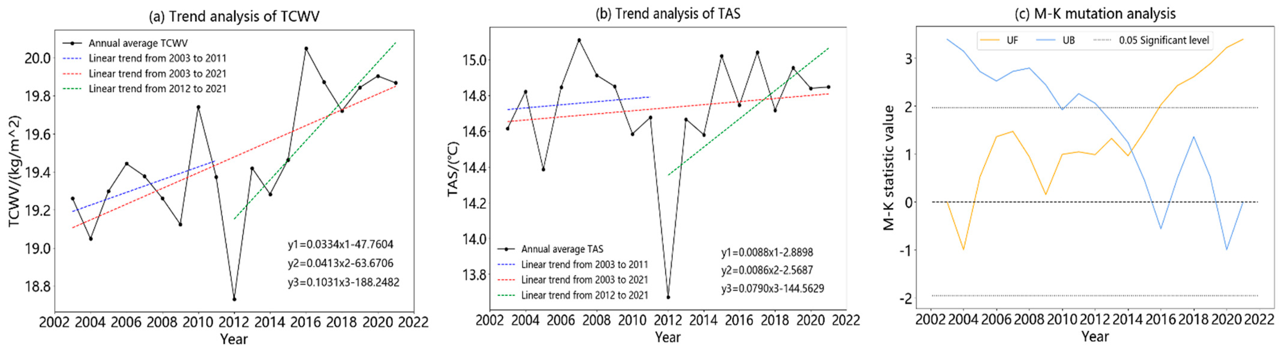
3.2.1. The Annual Variation Characteristics and Abrupt Change Analysis of TCWV in China

The trend analysis was performed on time series of a 19-year average of TCWV and TAS. For the data series y (t), t = 1, 2, 3, …, n is fitted by linear function $Y=a\times t+b$, and the constants A and B can be obtained by the least square method. In which a is not only a trend term, but also a direction that the time series changes with time, and a positive value indicates that its value has an increasing trend with time, negative value indicates a decreasing trend. Its absolute value indicates its degree of change. The M-K mutation test method was used to analyze the annual average TCWV in China, and the UF and UB curves of M-K mutation test were drawn.

The temporal variation and linear trend of the annual mean TCWV in China from 2003 to2021 can be seen in Figure 4a, which can be divided into two distinct stages. The blue dotted line shows the linear trend of TCWV from 2003 to 2011, and the analysis shows that the TCWV increases slowly at a rate of 0.03343 kg/m²/a. The green dotted line shows the linear trend of TCWV from 2012 to 2021, and the analysis shows that the TCWV increases at a rate of 0.1031kg/m²/a during this period. From the overall trend, that is the red dotted line, the TCWV in China shows a positive linear trend, and slowly increases at a rate of 0.0413 kg/m²/a. The phenomenon may be related to the long-term increase in temperature in recent years [38]. It can also be seen from Figure 4a that the maximum value 20.04 kg/m² appeared in 2016, the minimum value 18.73 kg/m² appeared in 2012, and the difference between the maximum and minimum values is 1.31 kg/m².

The linear change trend of TAS as shown in Figure 4b is similar to that of TCWV. The blue dotted line shows the linear trend of TAS from 2003 to 2011, the green dotted line shows the linear trend of TAS from 2012 to 2021, and the red dotted line shows the overall linear trend of TAS from 2003 to 2021. The TAS in each of the three time periods shows a positive linear trend. That is, the long-term increase in TAS in recent years has led to a slow increase in TCWV, which is consistent with the above description.

The M-K mutation test method was used to analyze the annual average TCWV in China, and the UF and UB curves of the M-K mutation test were plotted. It can be seen from Figure 4c that the time series of annual average TCWV in China from 2003 to 2021 is at the 0.05 significance level of an M-K mutation test, and there is an intersection between UF statistics and UB statistics in 2014, indicating that 2014 is the year of significant mutation of the annual TCWV series. The corresponding UF value is greater than 0, indicating that the intersection is the mutation point of the rise in annual average TCWV. From 2003 to 2005, UF values were less than 0, indicating a downward trend in TCWV; after 2005, the UF values were greater than 0, indicating an upward trend in TCWV during this period; after 2017, the UF values were greater than 1.96, indicating that the trend of the increase in the average TCWV during this period was obvious.

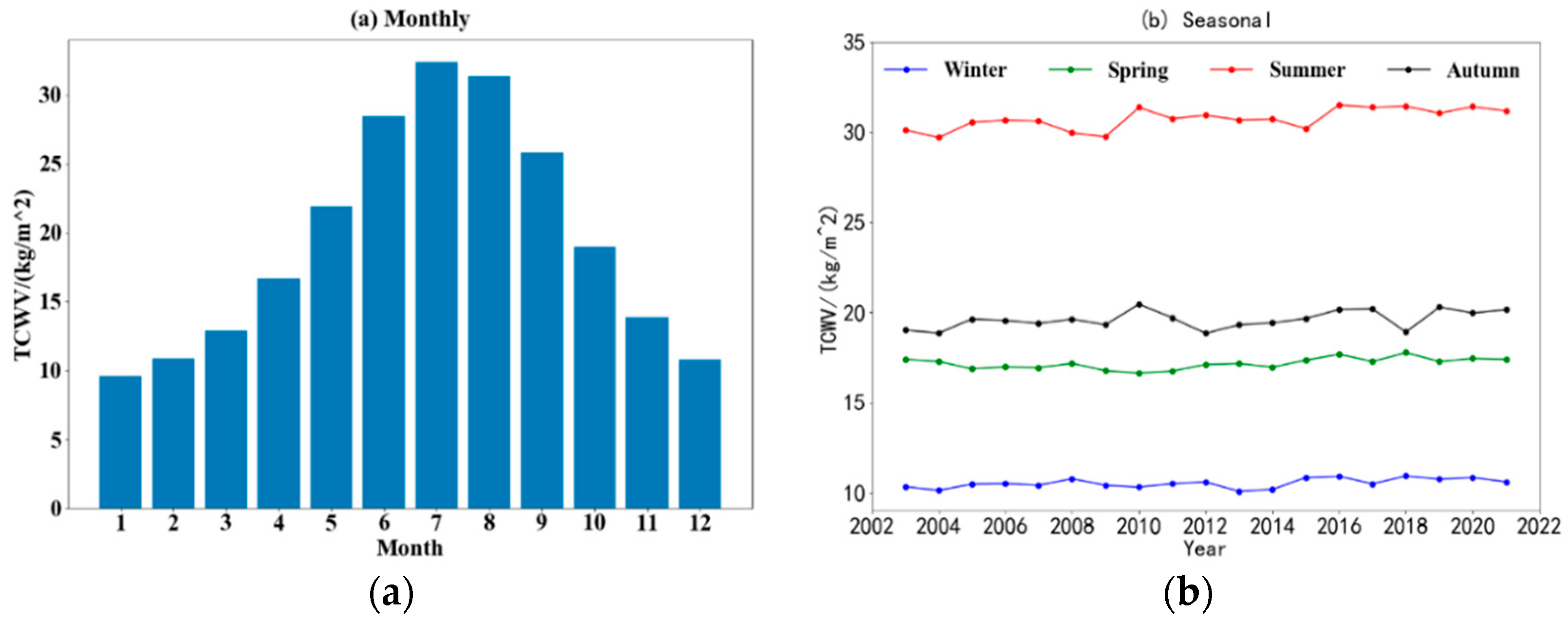
3.2.2. Monthly, Seasonal Variation Characteristics and Abrupt Change Analysis of TCWV in China

The monthly change of TCWV in China from September 2002 to February 2022 was analyzed. As shown in Figure 5a, its distribution is a slightly positive ‘bell-shaped’ curve. The TCWV gradually increased from January (9.58 kg/m²), reached the peak in July (32.37 kg/m²), then slightly decreased to 31.38 kg/m² in August, and then gradually decreased after September. The TCWV of China is mainly concentrated from May to September, and the total TCWV in these five months is 139.96 kg/m², accounting for about 59.90% of the annual TCWV. The TCWV in the other seven months is relatively low, among which January, February and December are all below 11 kg/m², which are 9.58 kg/m², 10.89 g/m² and 10.77 kg/m², respectively. The seasonal change of TCWV in of China from 2003 to 2021 was analyzed, and the seasonal variation of TCWV was shown in Figure 5b. It can be seen from Figure 5b that the TCWV in summer fluctuated around 30 kg/m², with a multi-year average of 30.73 kg/m². The annual averages of TCWV in spring and winter were 17.16 kg/m² and 10.52 kg/m², respectively. Therefore, it is concluded that the TCWV is most abundant in summer, relatively less in autumn and spring, and the least in winter, and the annual variation of TCWV in each season shows irregular changes.

The M-K mutation test method was used to test the seasonal average TCWV in China, and the UF and UB curves of the M-K mutation test were drawn. The M-K statistical curve (Figure 6a) of the winter TCWV in China was analyzed. The UF was greater than 0 after 2005, indicating that the winter TCWV showed an increasing trend after 2005. The UF and UB curves have intersections in 2015 and 2017, respectively, and the corresponding UF values are greater than 0 and between the two critical lines, but it cannot be stated which intersection is the mutation point of the TCWV rise in winter. The M-K statistical curve of the spring TCWV (Figure 6b) showed that the UF curve of spring TCWV in China was greater than 0 after 2015, indicating that the spring TCWV showed an increasing trend after 2015. The UF and UB curves had an intersection point during 2015, corresponding to the UF value between the two critical lines, indicating that the spring TCWV had a mutation in 2015. From the M-K statistical curve of TCWV in summer (Figure 6c), the UF curve showed an increasing trend, and the increasing trend was obvious, and the UF value was greater than 1.96 after 2016, indicating that the increasing trend of average TCWV in summer was obvious. The UF and UB curves had an intersection point in 2011 and the UF value was between the two critical lines, indicating that the TCWV had a mutation in the summer of 2011. It can be seen from Figure 6d that the UF of TCWV in autumn in China was greater than 0 after 2005, indicating that the average TCWV in autumn gradually increased after 2005. The UF and UB curves had multiple intersections from 2007 to 2015, and the corresponding UF values were greater than 0, although it cannot be determined which point is the mutation point.

3.2.3. Prediction of TCWV in China Based on SARIMA

The SARIMA model was used to predict the TCWV in China, and the monthly average value of TVWV from September 2002 to February 2022 was used as the original sample. The time series diagram and autocorrelation partial correlation diagram of TCWV are shown in Figure 7, and the lag of the autocorrelation coefficient in Figure 7 is set to 45. It can be seen from Figure 7 that the variation range of TCWV data is 10~35 kg/m². The Dickey-Fuller (DF) unit root test was performed on it, and a p-value = 0.39810 was obtained, meaning that the data accepted the null hypothesis, which implies that the data are non-stationary. Seasonal fluctuations in a time series can lead to the non-stationarity of a time series, which can be analyzed by constructing a SARIMA model. Therefore, seasonal difference and first-order difference were performed on the time series to make the data become stable.

The seasonal difference of the original time series is shown in Figure 8. A simple subtraction operation is performed on the sequence, and the time difference is the seasonal cycle (here we set the seasonal cycle to 12, because a year is 12 months). It can be seen from Figure 8 that p = 0.00002, which is much less than 0.05; that is, the data is a stationary series, which means that the seasonality is eliminated. It can be seen from the autocorrelation partial correlation diagram in Figure 8 that the series still has significant time lags, so we continue to perform differential processing on the series.

The first-order difference processing is performed on the time sequence, as shown in Figure 9, and the obtained p-value = 0, that is, the sequence is a stationary sequence. Then we perform a white noise test on it. This paper also uses the unit root test method, which in this particular case is the DF unit root test. The p-values obtained are far less than 0.01, 0.05, and the test is passed. That is, the obtained sequence is a stationary time series and a non-white noise sequence. By observing Figure 9, it can be preliminarily assumed that p = 3, because in the partial autocorrelation function (PACF) diagram, the maximum lag value that can be observed; since the first-order difference is made, assume that d = 1; because the 12th-order lag is obvious in the autocorrelation function (ACF) diagram, assume that Q = 1. Finally, the trial and error method is used near the initially determined parameters, and the final parameters are determined according to the principle of Akaike Information Criterion (AIC) minimum, and the final time series prediction model of monthly average TCWV in China is determined as SARIMA (3, 1, 3) × (0, 1, 1, 12).

The residual test was carried out on the stablished SARIMA model, and the autocorrelation graph test was used in this paper. As shown in Figure 10, except when lag = 0 oversteps 95% confidence interval, the rest are in the confidence interval. This shows that the fitting effect of the model is relatively good, and the original time series data can be understood and the future numerical value can be predicted.

The timing diagram of the finally drawn prediction sequence is shown in Figure 11. The abscissa represents the month, and the ordinate represents the values of TCWV. The blue curve is the true value, the red curve is the predicted value, and the red curve of the shadow part is the monthly average trend of TCWV in the next full year. It can be seen from Figure 11 that the predicted values are in good agreement with the actual ones. Furthermore, the mean absolute percentage error (MAPE), mean square error (MSE) and R²-score were calculated to judge the SARIMA model. The MAPE is 2.65%, MSE is 0.3229 and R²-score is 0.9949. This means that the prediction model is relatively accurate.

4. Discussions

Water vapor is one of the main greenhouse gases and has an important contribution to the greenhouse effect, accounting for about 60–80% of it, which is significantly higher than other greenhouse gases. Theoretically, the increase in temperature and the water vapor content have a mutual feedback effect. Global warming will lead to an increase in water vapor content, and the increase of water vapor will promote the enhancement of the greenhouse effect, thereby leading to global warming. In this paper, the SST data of China from 2002 to 2022 provided by AIRS were used. Considering that the TCWV is highly related to SST, the Pearson correlation coefficients of TCWV with SST were calculated (Figure 12a). A strong correlation existed between TCWV and SST with a correlation value of 0.93. Many studies have shown that TCWV is highly influenced by SST [39,40]. Figure 12b shows the spatial distribution of the average SST in China over the past 20 years. Its distribution is high in the east and low in the west, high in the south and low in the north, which has a high similarity with the spatial distribution of the TCWV.

Thus, the higher the temperature, the higher the corresponding water vapor. The reason is mainly determined by the Clausis-Clayperon equation. The higher the temperature, the stronger the water storage capacity of the atmosphere [41].

As one of the most important components of the lower atmosphere, water vapor is a necessary condition for the formation and evolution of weather and climate phenomena such as precipitation and is also an important factor affecting the generation and development of extreme weather. Studying the temporal and spatial variation of water vapor is an important aspect of studying climate change, which is of great significance to further understand the working mechanism of the entire climate and weather system. In this paper, we studied and analyzed the spatial-temporal, inter-annual and seasonal distribution of TCWV in China based on AIRS data. We also used the SARIMA model to extract sufficient information from the time series system using the time factor as a comprehensive factor to analyze and predict the monthly average changes of TCWV in China.

In China, studies have shown that the changes of water vapor not only have a greater correlation with the occurrence of droughts and floods in China, but the changes in water vapor affect the distribution of water resources in China. Therefore, an in-depth understanding of the temporal and spatial distribution of water vapor not only helps to study the impact mechanism of regional climate change under the background of global warming, but also provides a theoretical basis for the effective utilization of atmospheric water resources.

The EOF analysis has been used by experts and scholars in recent years to further investigate water vapor. In this study, we conducted the EOF analysis on the annual average TCWV from 2003 to 2021. It was found that the first variance contribution of the EOF analysis of TCWV is 31.47%, and the cumulative variance contribution of the first three modes is 59.73%, which means that the spatial distribution of the first three eigenvectors can represent the main distribution of water vapor content throughout the year. Jiang et al. [42] performed an EOF analysis on the precipitation in east China. The result showed the leading EOF pattern with an explained variance of 16%. There is also a clear dipole structure with the positive phase in the north and the negative phase in the south. The correlation coefficient between the series of leading principal component series and precipitation is 0.75, with a confidence level of exceeding 99%. Therefore, the first EOF is a good representation of precipitation variability in northern China. In Jia, X.J [43] ‘s EOF analysis of the spring (April–May) precipitation over China (SPC), the first EOF mode of SPC variation and the second EOF mode of SPC variation account for 27% and 18%, respectively, of the total variance from 1951–2014. Therefore, it shows that the EOF analysis modes of water vapor in different regions and seasons have different characteristics, which may require further research in the future.

5. Summary

In this paper we conducted an intensive analysis on spatiotemporal mode characteristics of TCWV in China during a recent 20-year period (2002–2022) based on the AIRS dataset and, furthermore, the trend of monthly mean time series over one entire year was predicted by using lows.

(1)

The annual and seasonal distribution of TCWV in China are roughly the same, and have obvious longitude and latitude distribution characteristics. That is, the variation trend of TCWV in China with longitude shows a “V” shape as a whole and the TCWV in China decreases with the increase of latitude. The spatial distribution of TCWV in China has an obvious southeast-northwest direction. Generally, the seasonal variation of the TCWV in the same area is summer > autumn > spring > winter.

(2)

By performing EOF decomposition of the TCWV in China, the contribution rate of variance of the first mode is 31.47%, indicating that it can reflect the typical spatial distribution pattern of the TCWV in China, that is, the positive distribution from southeast to northwest.

(3)

The TCWV in China showed an overall growth trend, and the M-K mutation test found that there was a significant mutation after 2014. After 2017, the UF value was greater than 1.96, and the upward trend was more obvious. The monthly variation curve shows a slightly positive deviation of the ‘bell-shaped’ curve, while the four seasons M-K curve shows that each has different mutation points.

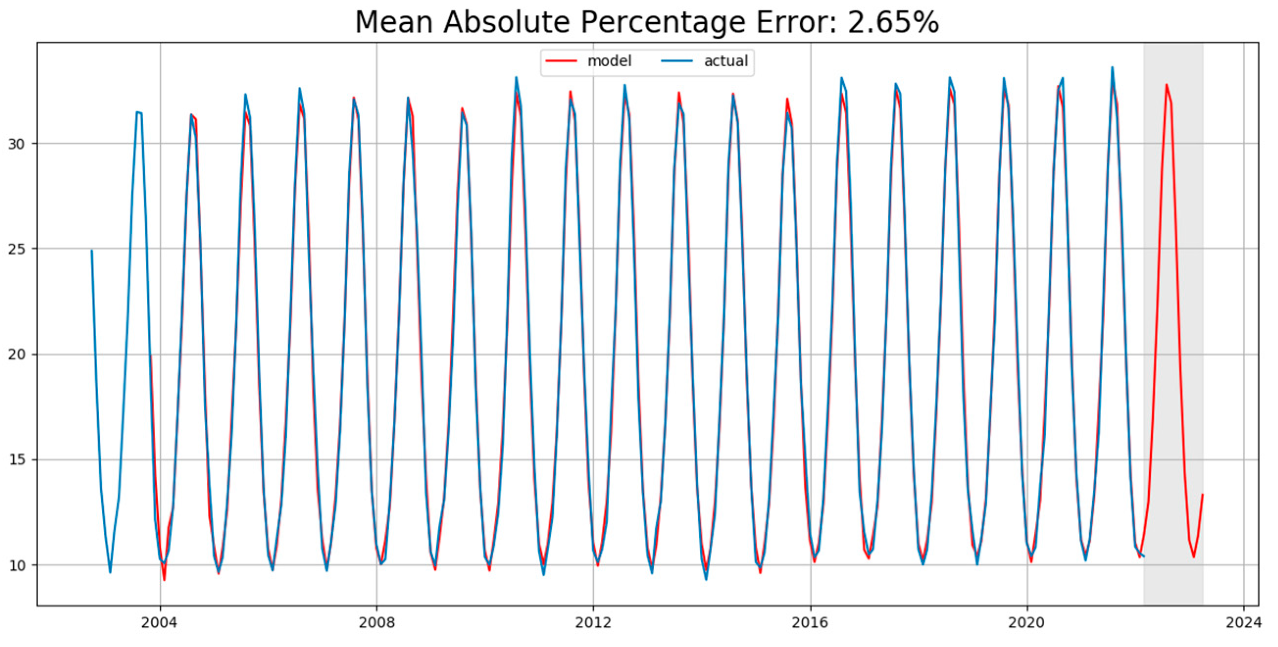
(4)

Using the SARIMA model, considering the trend and seasonality of TCWV time series, the optimal model is obtained. The average absolute error percentage (MAPE), mean square error (MSE), and R2-score are 2.65%, 0.3229 and 0.9949, respectively.

In this study, the spatiotemporal mode characteristics of TCWV were analyzed in China. These results validate the applicability and reliability of TCWV studies using the EOF, the Mann-Kendall test method. An increasing trend of TCWV in China has been observed from the analysis of the AIRS dataset. It has been illustrated that the upward trend of TCWV is becoming more apparent in recent years, which is likely due to various factors including anthropogenic global warming, large-scale moisture convergence, and dynamics. This paper includes a detailed study and analysis of SARIMA in forecasting time series data. The time model SARIMA can reflect the linear characteristics of time series data, and the model adds seasonality to the ARIMA model. Therefore, it can fit and predict the TCWV variation relatively accurately because of the added influence of seasonal factors on TCWV variation. These results provide a reference for understanding the characteristics of the global water cycle.

References

1. Varamesh, S.; Hosseini, S.M.; Rahimzadegan, M. Estimation of atmospheric water vapor using MODIS data. J. Mater. Environ. Sci. 2017, 8, 1690–1695. [Google Scholar]
2. Moradizadeh, M.; Momeni, M.; Saradjian, M.R. Estimation and validation of atmospheric water vapor content using a MODIS NIR band ratio technique based on AIRS water vapor products. Arab. J. Geosci. 2014, 7, 1891–1897. [Google Scholar] [CrossRef]
3. Chang, L.; Gao, G.; Li, Y.; Zhang, Y.; Zhang, C.; Feng, G. Variations in water vapor from AIRS and MODIS in response to Arctic sea ice change in December 2002–November 2016. IEEE Trans. Geosci. Remote Sens. 2019, 57, 7395–7405. [Google Scholar] [CrossRef]
4. Skliris, N.; Zika, J.D.; Nurser, G.; Josey, S.A.; Marsh, R. Global water cycle amplifying at less than the Clausius-Clapeyron rate. Sci. Rep. 2016, 6, 38752. [Google Scholar] [CrossRef] [PubMed] [Green Version]
5. Raval, A.; Ramanathan, V. Observational determination of the greenhouse effect. Nature 1989, 342, 758–761. [Google Scholar] [CrossRef]
6. Wang, Y.; Tang, L.; Gao, T.; Wang, Q.; Lu, C.; Song, Y.; Hua, D. Investigation and Analysis of All-Day Atmospheric Water Vapor Content over Xi’an Using Raman Lidar and Sunphotometer Measurements. Remote Sens. 2018, 10, 951. [Google Scholar] [CrossRef] [Green Version]
7. Held, I.M.; Soden, B.J. Robust Responses of the Hydrological Cycle to Global Warming. J. Clim. 2006, 19, 5686–5699. [Google Scholar] [CrossRef]
8. Wang, Z.; Sun, M.; Yao, X.; Zhang, L.; Zhang, H. Spatiotemporal Variations of Water Vapor Content and Its Relationship with Meteorological Elements in the Third Pole. Water 2021, 13, 1856. [Google Scholar] [CrossRef]
9. Gong, S.; Hagan, D.F.T.; Wu, X.; Wang, G. Spatio-temporal analysis of precipitable water vapour over northwest china utilizing MERSI/FY-3A products. Int. J. Remote Sens. 2018, 39, 3094–3110. [Google Scholar] [CrossRef]
10. Lu, J.; Xie, F.; Sun, C.; Luo, J.; Cai, Q.; Zhang, J.; Li, J.; Tian, H. Analysis of factors influencing tropical lower stratospheric water vapor during 1980–2017. Npj Clim. Atmos. Sci. 2020, 3, 35. [Google Scholar] [CrossRef]
11. Li, Z.; Liu, H. Temporal and Spatial Variations of Precipitation Change from Southeast to Northwest China during the Period 1961–2017. Water 2020, 12, 2622. [Google Scholar] [CrossRef]
12. Su, T.; Feng, G. The characteristics of the summer atmospheric water cycle over China and comparison of ERA-Interim and MERRA reanalysis. Acta Phys. Sin. 2014, 63, 249201. [Google Scholar] [CrossRef]
13. Hao, W.; Jianxin, H. Temporal and Spatial Evolution Features of Precipitable Water in China during a Recent 65-Year Period (1951–2015). Adv. Meteorol. 2017, 2017, 9156737. [Google Scholar] [CrossRef]
14. Zhao, Y.; Zhou, T. Asian water tower evinced in total column water vapor: A comparison among multiple satellite and reanalysis data sets. Clim. Dyn. 2020, 54, 231–245. [Google Scholar] [CrossRef] [Green Version]
15. Tuo, W.; Zhang, X.; Song, C.; Hu, D.; Liang, T. Annual precipitation analysis and forecasting–taking Zhengzhou as an example. Water Supply 2020, 20, 1604–1616. [Google Scholar] [CrossRef] [Green Version]
16. Hellen, W.K.; John, M.K.; George, O.O.; Yodah, W.O. Forecasting Precipitation Using SARIMA Model: A Case Study of Mt. Kenya Region. Math. Theory Modeling 2014, 4, 50–58. [Google Scholar]
17. Valipour, M. Long-term runoff study using SARIMA and ARIMA models in the United States. Meteorol. Appl. 2015, 22, 592–598. [Google Scholar] [CrossRef]
18. Alraddawi, D.; Sarkissian, A.; Keckhut, P.; Bock, O.; Noël, S.; Bekki, S.; Irbah, A.; Meftah, M.; Claud, C. Comparison of total water vapour content in the Arctic derived from GNSS, AIRS, MODIS and SCIAMACHY. Atmos. Meas. Tech. 2018, 11, 2949–2965. [Google Scholar] [CrossRef] [Green Version]
19. Parkinson, C.L. Aqua: An Earth-Observing Satellite mission to examine water and other climate variables. IEEE Trans. Geosci. Remote Sens. 2003, 41, 173–183. [Google Scholar] [CrossRef]
20. Tobin, D.C.; Revercomb, H.E.; Knuteson, R.O.; Lesht, B.M.; Larrabee Strow, L.L.; Hannon, S.E.; Feltz, W.F.; Moy, L.A.; Fetzer, E.J.; Cress, T.S. Atmospheric Radiation Measurement site atmospheric state best estimates for Atmospheric Infrared Sounder temperature and water vapor retrieval validation. J. Geophys. Res. Atmos. 2006, 111, 17884115. [Google Scholar] [CrossRef] [Green Version]
21. Liu, J.; Hagan, D.F.T.; Liu, Y. Global land surface temperature change (2003–2017) and its relationship with climate drivers: Airs, MODIS, and ERA5-land based analysis. Remote Sens. 2020, 13, 44. [Google Scholar] [CrossRef]
22. Bi, S.; Qiu, X.; Wang, G.; Gong, Y.; Wang, L.; Xu, M. Spatial distribution characteristics of drought disasters in Hunan Province of China from 1644 to 1911 based on EOF and REOF methods. Environ. Earth Sci. 2021, 80, 533. [Google Scholar] [CrossRef]
23. Qinzheng, L.; Peng, C.; Sun, L.; Ma, X. A global weighted mean temperature model based on empirical orthogonal function analysis. Adv. Space Res. 2018, 61, 1398–1411. [Google Scholar] [CrossRef]
24. Fu, D.; Huang, Y.; Liu, D.; Liao, S.; Yu, G.; Zhang, X. Analysis of the regional spectral properties in northwestern South China Sea based on an empirical orthogonal function. Acta Oceanol. Sin. 2020, 39, 107–114. [Google Scholar] [CrossRef]
25. Ayantobo, O.O.; Wei, J.; Kang, B.; Li, T.; Wang, G. Spatial and temporal characteristics of atmospheric water vapour content and its relationship with precipitation conversion in China during 1980–2016. Int. J. Climatol. 2021, 41, 1747–1766. [Google Scholar] [CrossRef]
26. Kendall, M. A New Measure of Rank Correlation. Biometrika 1938, 30, 81–93. [Google Scholar] [CrossRef]
27. Shadmani, M.; Marofi, S.; Roknian, M. Trend Analysis in Reference Evapotranspiration Using Mann-Kendall and Spearman’s Rho Tests in Arid Regions of Iran. Water Resour. Manag. 2012, 26, 211–224. [Google Scholar] [CrossRef] [Green Version]
28. Fu, C.B.; Wang, Q. The definition and detection of the abrupt climate change. Atmos. Sci. 1992, 16, 482–492. [Google Scholar]
29. Xing, L.; Huang, L.; Chi, G.; Yang, L.; Li, C.; Hou, X. A dynamic study of a karst spring based on wavelet analysis and the Mann-Kendall Trend Test. Water 2018, 10, 698. [Google Scholar] [CrossRef] [Green Version]
30. Dubey, A.K.; Kumar, A.; García-Díaz, V.; Kumar Sharma, A.; Kanhaiya, K. Study and analysis of SARIMA and LSTM in forecasting time series data. Sustain. Energy Technol. Assess. 2021, 47, 101474. [Google Scholar] [CrossRef]
31. Song, Z.; Guo, Y.; Wu, Y.; Ma, J. Short-term traffic speed prediction under different data collection time intervals using a SARIMA-SDGM hybrid prediction model. PLoS ONE 2019, 14, e0218626. [Google Scholar] [CrossRef] [PubMed]
32. Wei, Y.; Melkumian, A.V. Forecasting Australian Red Wine Sales with SARIMA and ANNs. In Proceedings of the 2020 International Symposium on Frontiers of Economics and Management Science (FEMS 2020), Dalian, China, 20–21 March 2020; Wuhan University of Technology: Wuhan, China, 2020; pp. 147–151. [Google Scholar] [CrossRef]
33. Yaya, O.S.; Fashae, O.A. Seasonal fractional integrated time series models for rainfall data in Nigeria. Theor. Appl. Climatol. 2015, 120, 99–108. [Google Scholar] [CrossRef]
34. Hu, Y.; Wang, N.; Liu, S.; Jiang, Q.; Zhang, N. Application of time series model and LSTM model in water quality prediction. Miniat. Microcomput. Syst. 2022, 42, 5. [Google Scholar]
35. Dimri, T.; Ahmad, S.; Sharif, M. Time series analysis of climate variables using seasonal ARIMA approach. J. Earth Syst. Sci. 2020, 129, 149. [Google Scholar] [CrossRef]
36. Moeeni, H.; Bonakdari, H.; Ebtehaj, I. Monthly reservoir inflow forecasting using a new hybrid SARIMA genetic programming approach. J. Earth Syst. Sci. 2017, 126, 18. [Google Scholar] [CrossRef]
37. Wypych, A.; Bochenek, B.; Różycki, M. Atmospheric moisture content over Europe and the Northern Atlantic. Atmosphere 2018, 9, 18. [Google Scholar] [CrossRef] [Green Version]
38. Tian, Y.; Yan, Z.; Li, Z. Spatial and Temporal Variations of Extreme Precipitation in Central Asia during 1982–2020. Atmosphere 2021, 13, 60. [Google Scholar] [CrossRef]
39. Gaffen, D.J.; Elliott, W.P.; Robock, A. Relationships between tropospheric water vapor and surface temperature as observed by radiosondes. Geophys. Res. Lett. 1992, 19, 1839–1842. [Google Scholar] [CrossRef] [Green Version]
40. Zhang, J.; Zhao, T. Historical and future changes of atmospheric precipitable water over China simulated by CMIP5 models. Clim. Dyn. 2019, 52, 6969–6988. [Google Scholar] [CrossRef]
41. Xu, X.; Lu, C.; Shi, X.; Gao, S. World water tower: An atmospheric perspective. Geophys. Res. Lett. 2008, 35, L20815. [Google Scholar] [CrossRef]
42. Jiang, Z.; Jiang, S.; Shi, Y.; Liu, Z.; Li, W.; Li, L. Impact of moisture source variation on decadal-scale changes of precipitation in North China from 1951 to 2010. J. Geophys. Res. Atmos. 2017, 122, 600–613. [Google Scholar] [CrossRef]
43. Jia, X.J.; You, Y.J.; Wu, R.G.; Yang, Y. Interdecadal changes in the dominant modes of the interannual variation of spring precipitation over China in the mid-1980s. J. Geophys. Res. Atmos. 2019, 124, 10676–10695. [Google Scholar] [CrossRef]
Figure 1. Spatial distribution of TCWV during 2002–2022 in China. (a) Longitude distribution. (b) Latitude distribution. (c) Longitude and latitude distribution.
Atmosphere 13 00885 g001
Figure 2. TCWV of China in each season. (a) Winter. (b) Spring. (c) Summer. (d) Autumn.
Atmosphere 13 00885 g002
Figure 3. (a,c,e) Spatial distribution of EOF of the TCWV, and (b,d,f) corresponding normalized principle component (PC).
Atmosphere 13 00885 g003
Figure 4. Interannual variation trend. (a) Trend analysis of TCWC. (b) Trend analysis of TAS. (c) M-K mutation analysis.
Atmosphere 13 00885 g004
Figure 5. Monthly and seasonal variation of TCWV in China (2003–2021). (a) Monthly. (b) Seasonal.
Atmosphere 13 00885 g005
Figure 6. Mann-Kendall statistic curve of TCWV in seasonal in China. (a) Winter. (b) Spring. (c) Summer. (d) Autumn.
Atmosphere 13 00885 g006
Figure 7. Time series, autocorrelation and partial autocorrelation of TCWV.
Atmosphere 13 00885 g007
Figure 8. Time series, autocorrelation and partial autocorrelation of TCWV after seasonal difference.
Atmosphere 13 00885 g008
Figure 9. Time series, autocorrelation and partial autocorrelation of TCWV after first-order difference.
Atmosphere 13 00885 g009
Figure 10. Residual test.
Atmosphere 13 00885 g010
Figure 11. Prediction result of SARIMA model.
Atmosphere 13 00885 g011
Figure 12. The relationship between TCWV and SST. (a) Correlation of TCWV with SST. (b) Distribution of SST in China.
Atmosphere 13 00885 g012
Publisher’s Note: MDPI stays neutral with regard to jurisdictional claims in published maps and institutional affiliations.