
Influence of the Grid Resolutions on the Computer-Simulated Surface Air Pollution Concentrations in Bulgaria


National Institute of Geophysics, Geodesy and Geography—Bulgarian Academy of Sciences, Acad. G. Bonchev Str., Bl. 3, 1113 Sofia, Bulgaria
*
Author to whom correspondence should be addressed.
Atmosphere 2022, 13(5), 774; https://doi.org/10.3390/atmos13050774
Submission received: 20 April 2022
/
Revised: 5 May 2022
/
Accepted: 9 May 2022
/
Published: 10 May 2022
(This article belongs to the Special Issue Atmospheric Composition and Regional Climate Studies in Bulgaria)
Abstract
:The present study aims to demonstrate the effects of horizontal grid resolution on the simulated pollution concentration fields over Bulgaria. The computer simulations are performed with a set of models used worldwide—the Weather Research and Forecasting Model (WRF)—the meteorological preprocessor, the Community Multiscale Air Quality Modeling System (CMAQ)—chemical transport model, Sparse Matrix Operator Kernel Emissions (SMOKE)—emission model. The large-scale (background) meteorological data used in the study were taken from the ‘NCEP Global Analysis Data’ with a horizontal resolution of 1° × 1°. Using the ‘nesting’ capabilities of the WRF and CMAQ models, a resolution of 9 km was achieved for the territory of Bulgaria by sequentially solving the task in several consecutive nested areas. Three cases are considered in this paper: Case 1: The computer simulations result from the domain with a horizontal resolution (both of the emission source description and the grid) of 27 km.; Case 2: The computer simulations result from the domain with a horizontal resolution (both of the emission source description and the grid) of 9 km.; Case 3: A hybrid case with the computer simulations performed with a grid resolution of 9 km, but with emissions such as in the 27 km × 27 km domain. The simulations were performed, for all the three cases, for the period 2007–2014 year, thus creating an ensemble large and comprehensive enough to reflect the most typical atmospheric conditions with their typical recurrence. The numerical experiments showed the significant impact of the grid resolution not only in the pollution concentration pattern but also in the demonstrated generalized characteristics. Averaged over a large territory (Bulgaria); however, the performances for cases one and two are quite similar. Bulgaria is a country with a complex topography and with several considerably large point sources. Thus, some of the conclusions made, though based on Bulgarian-specific experiments, may be of general interest.
1. Introduction
Over the last years, it became obvious that our understanding of pollution and exposure processes at the regional–local–urban scales could be improved by combining multiscale models and creating new dedicated numerical approaches and that the representation of different scale interactions of dynamic, pollutant emission sources and pollutant transformations would be a critical element in obtaining more realistic simulation results.
Meteorology is one of the main uncertainties of air quality modeling and prediction. Many studies have investigated the role of meteorology on air quality [1,2,3,4,5,6,7,8,9,10,11,12]. The relationship between meteorology and air pollution is a result of a complex interaction between the atmospheric circulation and physical and chemical processes of the air pollutants in both gas and aerosol form. The improvement of atmospheric composition prediction capability is, therefore, tied to progress in both fields and their coupling. Recently, two-way coupling has been widely recommended as a more appropriate approach.
It is still not proved, however, that, having in mind the uncertainties and errors in the raw meteorological input data, the refinement of the computational grid always leads to better simulations of the meteorological fields.
Successful air pollution modeling requires expert knowledge of air pollution sources regarding their strength, chemical characterization, spatial distribution, and temporal variation, along with knowledge of their atmospheric transport and processing. Unfortunately, emission inventories for many of the activity types (road transport, for example) usually contain only annual data, aggregated for countries or large areas. Atmospheric models, however, need hourly emission data for the grid cells of the model domain, furthermore the height of the emissions (above ground), and for non-methane volatile organic compounds (NMVOC), particulate matter (PM), and nitrogen oxides (NOx) a breakdown into species or classes of species according to the chemical scheme of the atmospheric model is necessary. For PM, information is also required on the size distribution. Thus, a transformation of the available data into structure and resolution as needed by the models has to be made [13].
Procedures for spatial disaggregation for several emission sectors by using different surrogates (population density, road network density, etc.) are recommended in chapter seven of the EMEP/EEA air pollutant emission inventory guidebook 2019 [14]. These proxy data are not always available in high spatial resolution, so applying very high horizontal model resolution may, therefore, generate false signals.
By all means, the horizontal grid resolution plays an immense role in the air pollution simulation results. There is a huge number of works, for example [15,16,17,18,19,20,21,22,23,24,25,26,27,28,29,30,31,32,33,34,35,36,37,38,39,40,41,42,43,44,45], dedicated to this subject. As stated in [46], these papers, in one way or another, are trying to answer the following questions:
1. To what extent the refining the horizontal grid resolution improves the performance of the models, not only in specific points but domain-wide?
2. How does fine resolution modeling influence spatial and temporal atmospheric composition patterns and the related metrics, evaluating environmental, human health, quality of life, etc., atmospheric composition impacts?
3. How does the resolution of specific model inputs (e.g., meteorology, emissions, topography, land use, etc.) impact the model outputs?
4. Which chemical transport model inputs provide a greater benefit to be of fine resolutions?
All these questions still do not have a definitive answer. Apparently, coarse modeling does not sufficiently display spatial atmospheric composition variance. Just as apparent, the results indicate that coarse modeled pollution concentrations underestimate maxima in urban areas and overestimate in rural areas. The resolution of meteorology and emissions impact different species to different extents. For example, generally, ozone (O3) was more impacted by meteorology, while NO2 and PM2.5 were more influenced by emissions.
Some studies indicate that, averaged over a large domain, quantities do not drastically change between coarse and fine resolution.
Though many of the above-cited papers demonstrate that grid refinement improves the simulation results, it can be stated that fine resolution modeling is not always reasonable, and one must consider the purpose of the analysis before assuming that fine-grid resolutions will improve overall results.
The present study does not aim at judging if grid refinement leads to more accurate atmospheric composition simulations. A modest task is to simply demonstrate the effects of horizontal grid resolution on the simulated pollution concentration fields over Bulgaria. It seems that Bulgaria is a good site for such an experiment because of the country’s complex topography and the presence of several considerably large point sources (mostly TPPs). Thus, some of the conclusions made, though based on Bulgarian-specific experiments, may be generally valid.
2. Materials and Methods
2.1. Modeling Tools
WRF v.3.2.1—Weather Research and Forecasting Model, [47], the meteorological preprocessor at CMAQ. The Weather Research and Forecasting Model (WRF) is a next-generation meso-scale numerical weather forecasting system designed to serve both operational forecasting and atmospheric research needs. It is the evolutionary successor to the MM5 model. The creation and further development of the WRF are due to the joint efforts of several US institutions such as NCAR, NOAA, NCEP, and others. WRF is a non-hydrostatic model with hydrostatic pressure coordinates following the terrain. The discretization is Arakawa-C type;
CMAQ v.4.6—chemical transport model with proven qualities, applied worldwide and in European practices, [48,49,50];
SMOKE—emission model. It should be noted that SMOKE is very strongly oriented toward the American methodology for determining emissions with its categorizations and databases. For this reason, its application for modeling the levels of pollutants in Europe and Bulgaria is relatively limited. Most often, European scientists use emission models created by themselves. Intensive work is underway in a number of research groups to adapt SMOKE to European conditions. So far, the use of this processor is partly mainly for estimating biogenic emissions, emissions from large point sources and merging the various emission files, and saving them in the necessary formats.
It is important to note that the choice of this system of models is due not only to their great popularity and highly rated simulation qualities but also to the fact that in recent years these models have been well validated [51] and largely used for computer simulations of atmospheric composition of the Balkan Peninsula and Bulgaria [52,53,54,55,56,57].
2.2. Meteorological Data
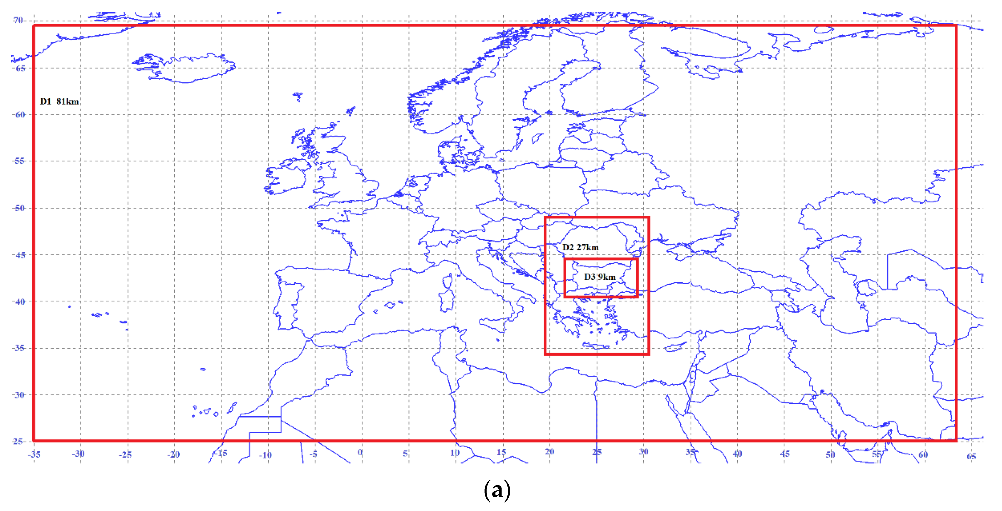
The large-scale (background) meteorological data used in the study were taken from the ‘NCEP Global Analysis Data’ with a horizontal resolution of 1° × 1°. Using the ‘nesting’ capabilities of the WRF and CMAQ models, a resolution of 9 km was achieved for the territory of Bulgaria by sequentially solving the task in several consecutive, nested areas (Figure 1a).
2.3. Emission Data and Emission Modeling
The detailed emission inventory made by TNO, the Netherlands [58] was used for the domains outside Bulgaria. The inventory of emissions is made on an annual basis. The pollutants were calculated in groups such as CH4, CO, NH3, NMVOC (non-methane VOC, VOC—volatile organic compounds), NOx, SOx, PM10, and PM2.5. The Bulgarian emissions are taken from the Bulgarian national emission inventory.
CMAQ, such as other chemical transport models, requires its input with emissions to be in a format that reflects the evolution over time of all pollutants involved in the chemical mechanism used. When preparing the input file for CMAQ, a number of additional procedures must be performed:
- First, all primary information must be interpolated into the corresponding selected network/networks (gridded);
- Second, time profiles should be imposed to modify the annual values so as to take into account seasonal, weekly, and daily variations in the work of the sources.
- Finally, emissions from the “families” of organic gases and, to a lesser extent, SOx, NOx, and PM2.5 must be split or “converted” into a larger number of components, according to the emission input requirements of CMAQ, which in turn depend on the chosen chemical mechanism—a procedure called “speciation”.
In doing so, each of the different types of sources: surface (AS), large point (LPS), and biogenic (BgS), should be treated in a specific way (emissions from transport are also a separate category, but due to the way they are inventoried in our country, they are combined with area sources). Obviously, emission models are preprocessors needed for chemical transformation and pollutant transport models. One such component is SMOKE. Unfortunately, as already noted, it is very much adapted to the conditions in the United States—emission inventories, administrative division, categorization, combustion processes, etc.
For the purposes of the present study, time variations in emissions were calculated on the basis of daily, weekly, and monthly profiles provided in [59,60]. These time profiles are country, pollutant, and SNAP (Selected Nomenclature for Air Pollution) specific.
The “speciation” procedure depends on the chemical mechanism used. CMAQ supports various chemical mechanisms. For the purposes of the present study, Carbon Bond v.4—CB4 is used [61].
A specific approach to this speciation has been developed. It is proposed to follow the technology developed by the US EPA Emission Factor and Inventory Group [62]. More details about the speciation procedure can be seen in [63].
The inputs needed to calculate emissions are gridded data for area sources (AS), large point sources (LPS), and land use data needed to model biogenic sources (BgS). The latter emits organic matter, CO and NO, and their values depend heavily on weather conditions, including sunshine.
The area source data are processed by the specially designed AEmis program, which performs speciation and time profiles for each network cell for each SNAP for the respective Julian dates. The obtained hourly values of all 22 pollutants (CH4, CO, NH3, 10 types VOC, NOx, SOx, PMC, and 5 types PM2.5) are saved in a file in NetCDF format.
The LPS database contains data for only 4 SNAP sectors—1, 3, 4, and 8. This information, together with the MCIP output, is fed to the SMOKE LPS processor, which produces the respective emission file. For this purpose, the inventory of powerful point sources is transformed into the requirements of SMOKE IDA format. This is a text file, but the order of the variables and their positions are fixed. This file, along with the inventory data, includes a number of parameters of the sources, such as geographical coordinates, height and diameter of the chimney, speed and temperature of discharge of pollutants, and more. The model not only performs speciation and time allocation but also calculates the so-called. “Plume-rise”—ejection of pollutants in height as a result of mechanical impulse and Archimedean forces. This increase in height also depends significantly on weather conditions—wind and atmospheric stability. As a result, SMOKE produces a 3D file—the pollutants are dumped at different levels (the levels coincide with the vertical structure of CMAQ).
SMOKE is also used to create a file with the third type of emissions—biogenic emissions. SMOKE currently supports the BEIS (Biogenic Emissions Inventory System) mechanism, versions 2 and 3 [64,65]. BEIS2 and BEIS3 are fed by the spatial distribution of the underlying surface type for the first step of the process—the calculation of normalized emissions for each network cell and for each underlying surface category (these are the emissions at fixed standard meteorological parameters). The final step is to bring normalized emissions up to date on the basis of grid and hourly meteorological information. The current version of SMOKE incorporates the BEIS3.13 mechanism [66].
Three cases are considered in this paper:
Case 1: The computer simulations result from D2—the domain with a horizontal resolution (both of the emission source description and the grid) of 27 km, projected into the D3 grid. This case will be further referred to as C1;
Case 2: The computer simulations result from D3—the domain with a horizontal resolution (both the emission source description and the grid) of 9 km. This case will be further referred to as C2;
Case 3: The results of the computer simulations performed in D3 with a grid resolution of 9 km, but with emissions such as in D2—the emissions from each of the 27 × 27 km grid points are divided into 9 and allocated to each of the 9 points from the D3 grid, contained in the respective D2 grid cell. Thus the total emission amount of each of the D2 grid points is preserved, only distributed equally to the neighboring D3 grid points. This case will be further referred to as C3.
The simulations were performed, for all the three cases, for the period 2007—2014 year, thus creating an ensemble large and comprehensive enough to reflect the most typical atmospheric conditions with their typical recurrence.
The emission sources were constructed on the basis of 2005 emission inventory. This was performed on purpose—at that time, the emissions from the thermal power plants (TPPs) in Bulgaria were not reduced yet, so the experiment can also follow the effects of very large elevated point sources.
3. Results
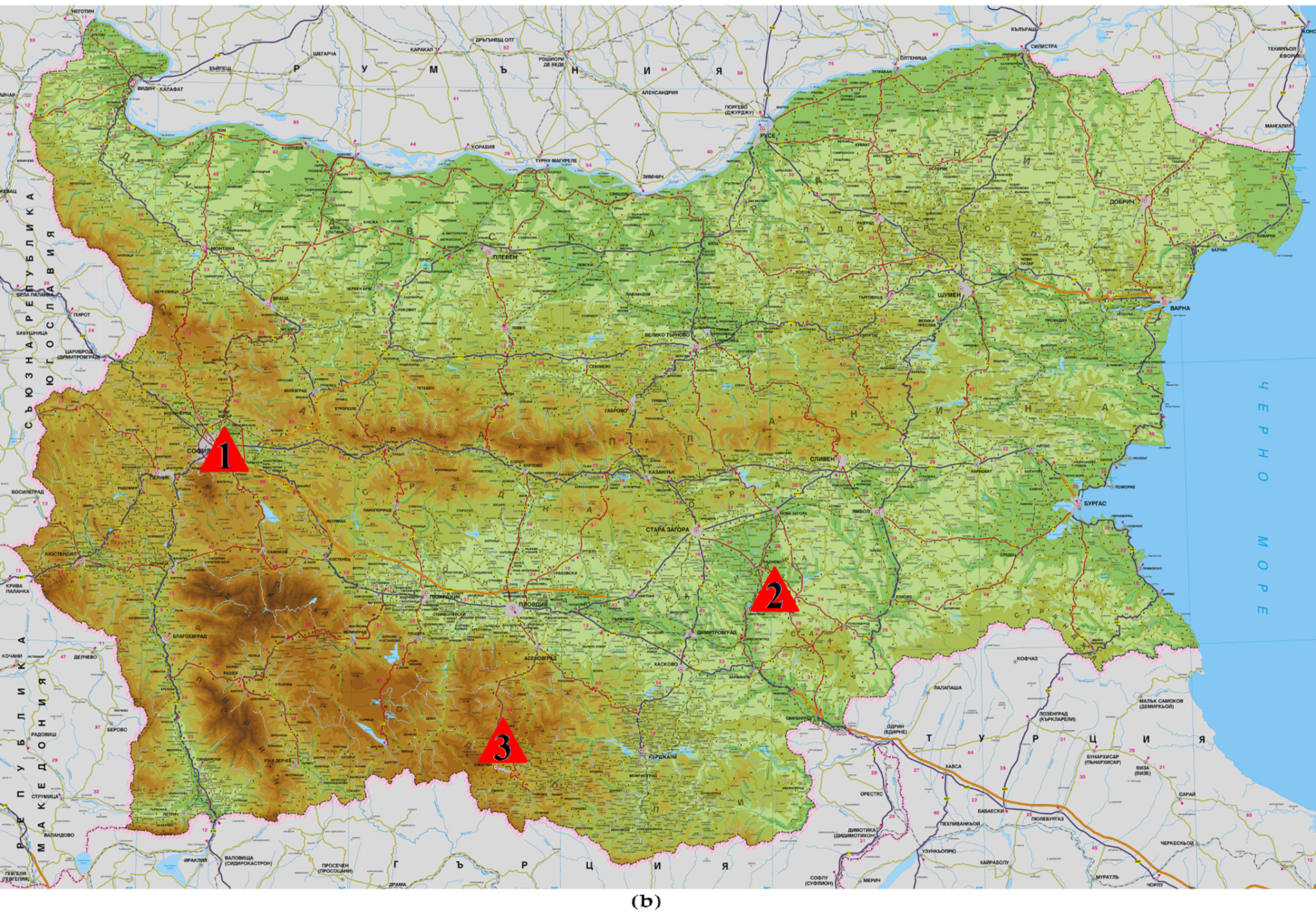
Maps of the surface annually-averaged concentrations of NO2 for cases C1, C2, and C3 are shown in Figure 2. The effect of the grid resolution is clearly manifested—the pattern of C2 is more detailed and displays the main road network and some of the big cities (large ground area sources). In the C3 fields, the local maximum near the southern border of Bulgaria can be noticed during the whole day. This probably is due to the emissions from Maritsa TPPs. This maximum is not observed in C1 and C2 fields, which suggests that it is perhaps created by the combined effects of coarse source description and detailed atmospheric dynamics and chemistry. The joint effect of coarse source description and detailed atmospheric dynamics and chemistry is also manifested by the fact that C3 fields are more diffused compared to C1 and C2 ones.
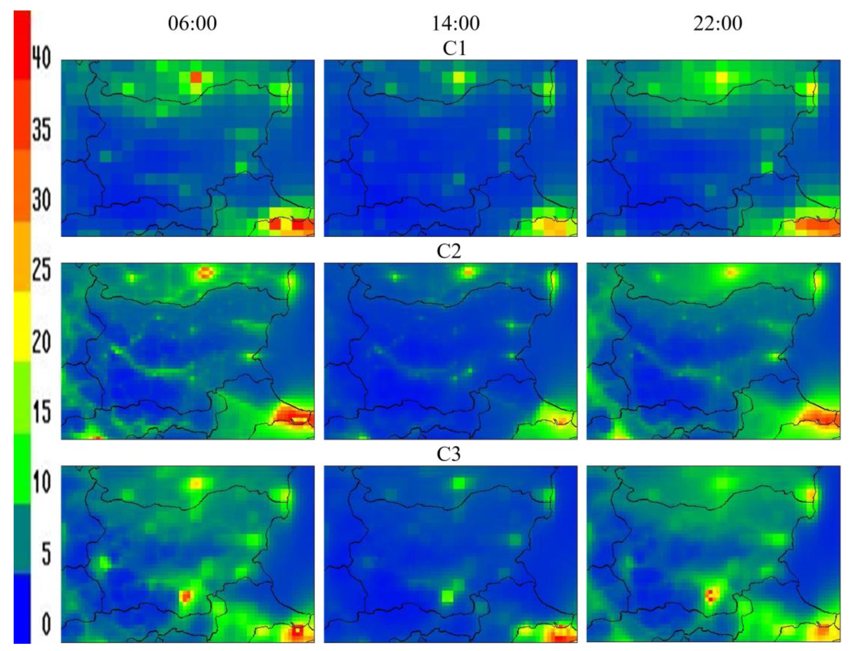
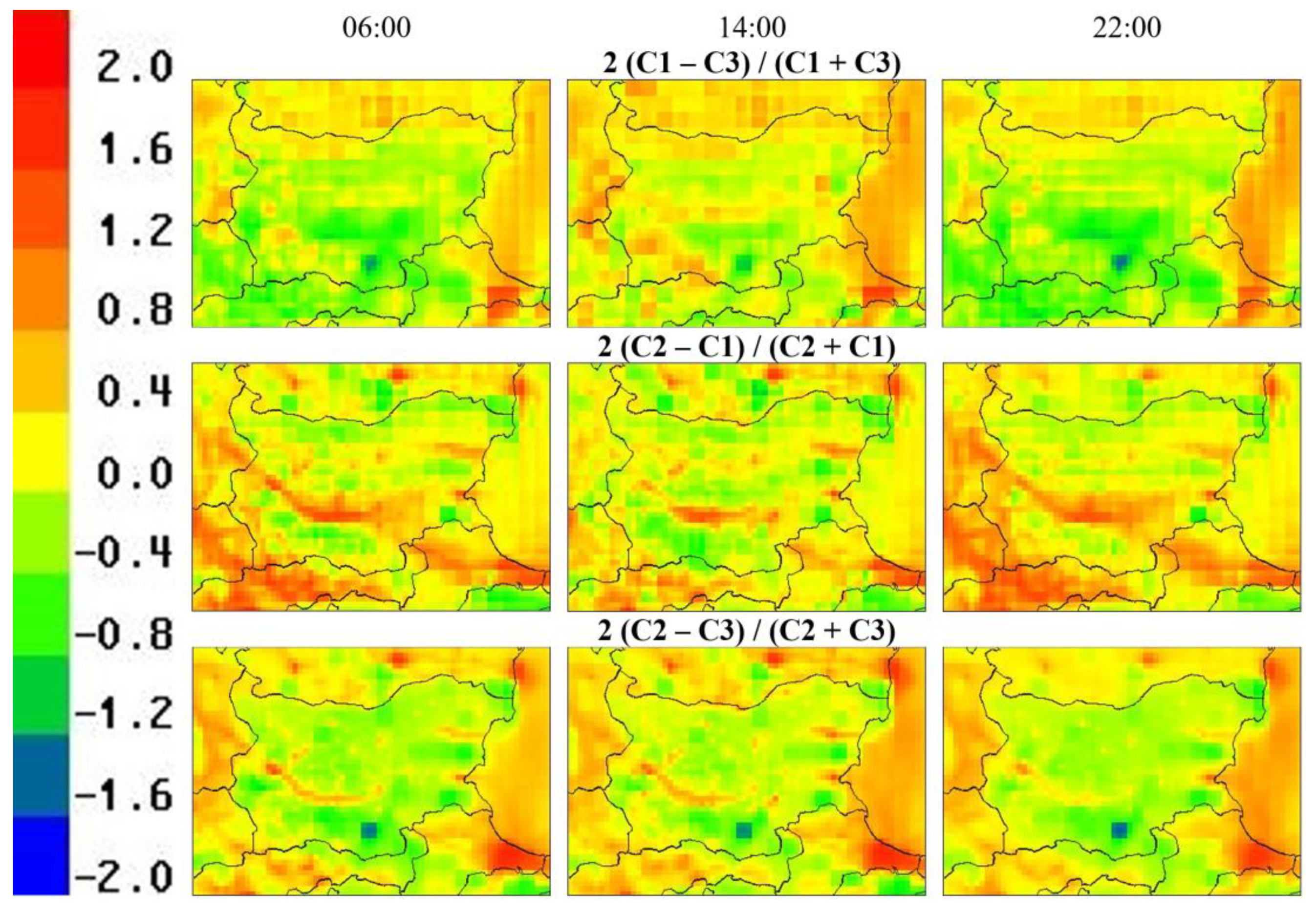
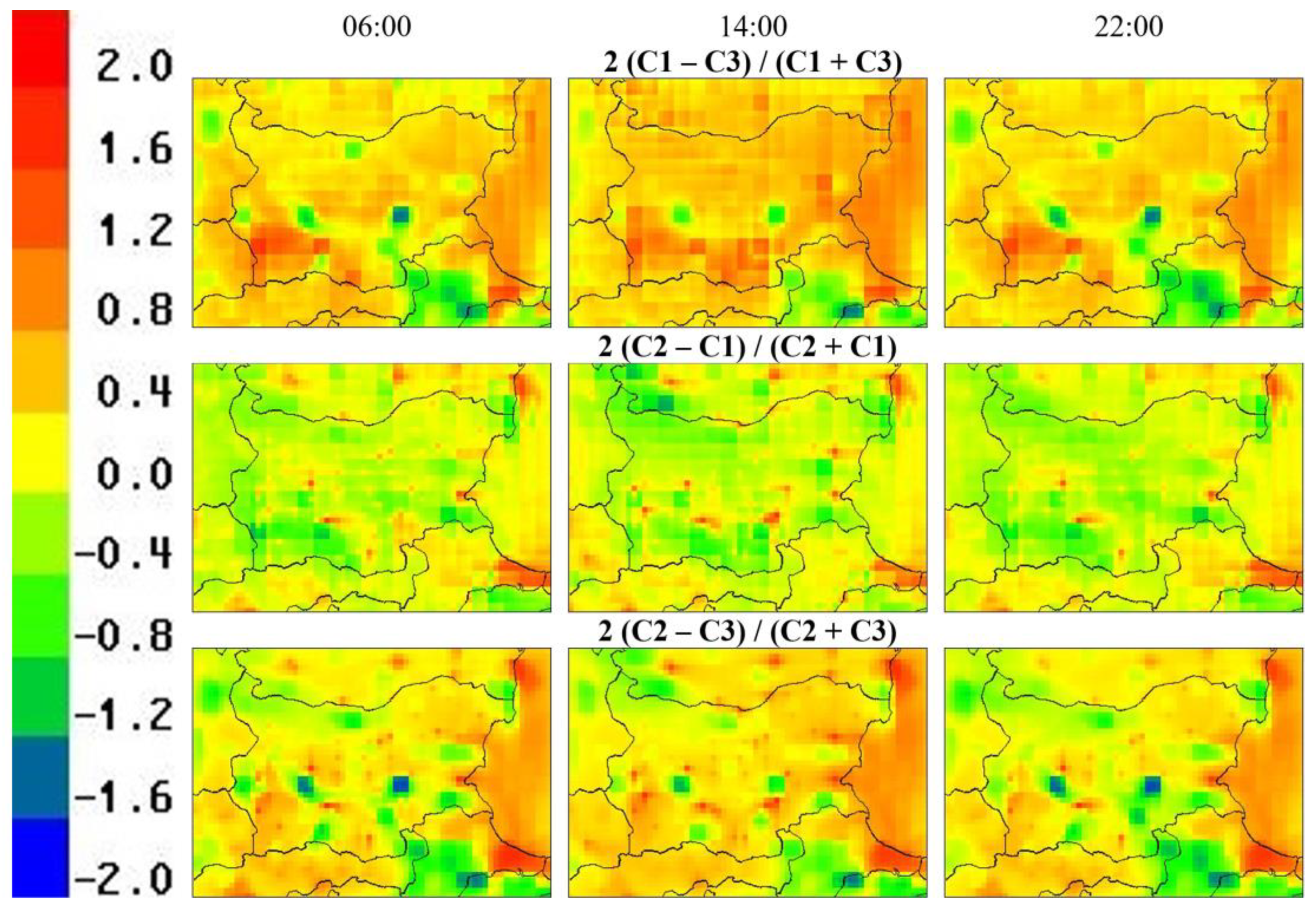
The grid resolution effects are very well manifested in the maps of the annually averaged relative differences of the surface concentrations for different cases (Figure 3, Figure 4, Figure 5 and Figure 6). The maps for NO2 virtually display the same effects as in Figure 2. It can be seen that the difference in the resolution of the road traffic emissions is also displayed in C2-C3 relative differences, but not so prominently as in C2-C1 relative differences. Due to the fact that the atmospheric dynamics in cases C2 and C3 are with the same resolution, the effect of the difference in the road traffic emission resolution is not so diffused and is concentrated near the main roads only.
The relative differences between cases C1 and C2 are big for larger areas, which suggests a cumulative effect of emission and dynamics resolution. At noon, the relative differences between C1 and C3 show large values above mountain regions. This clearly is an effect of differences in dynamic resolution.
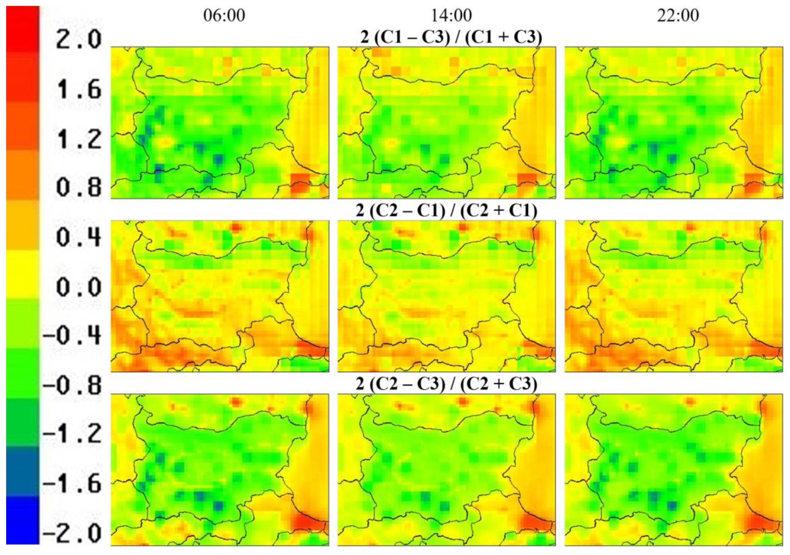
The relative differences for SO2 are shown in Figure 4. The most remarkable feature in C2-C1 cases is the small spots with positive, fairly large relative differences located close to large SO2 point sources—a clear effect of the emission source resolution. Significant local maximums and minimums can be seen for C1-C3 and C2-C3 cases, which probably is a result of the combined effects of emission source and atmospheric dynamic and chemistry resolution. Unlike the NO2 case, the larger relative differences for SO2 are between C1 and C3.
The biggest positive relative differences for PM2.5 (Figure 5) are between cases C2 and C1, and the biggest negative differences are between C1-C3 and C2-C3. The relative difference maps pattern shows the big positive differences are related to the road network and some area sources, while the big negative differences are related mostly to elevated large point sources.
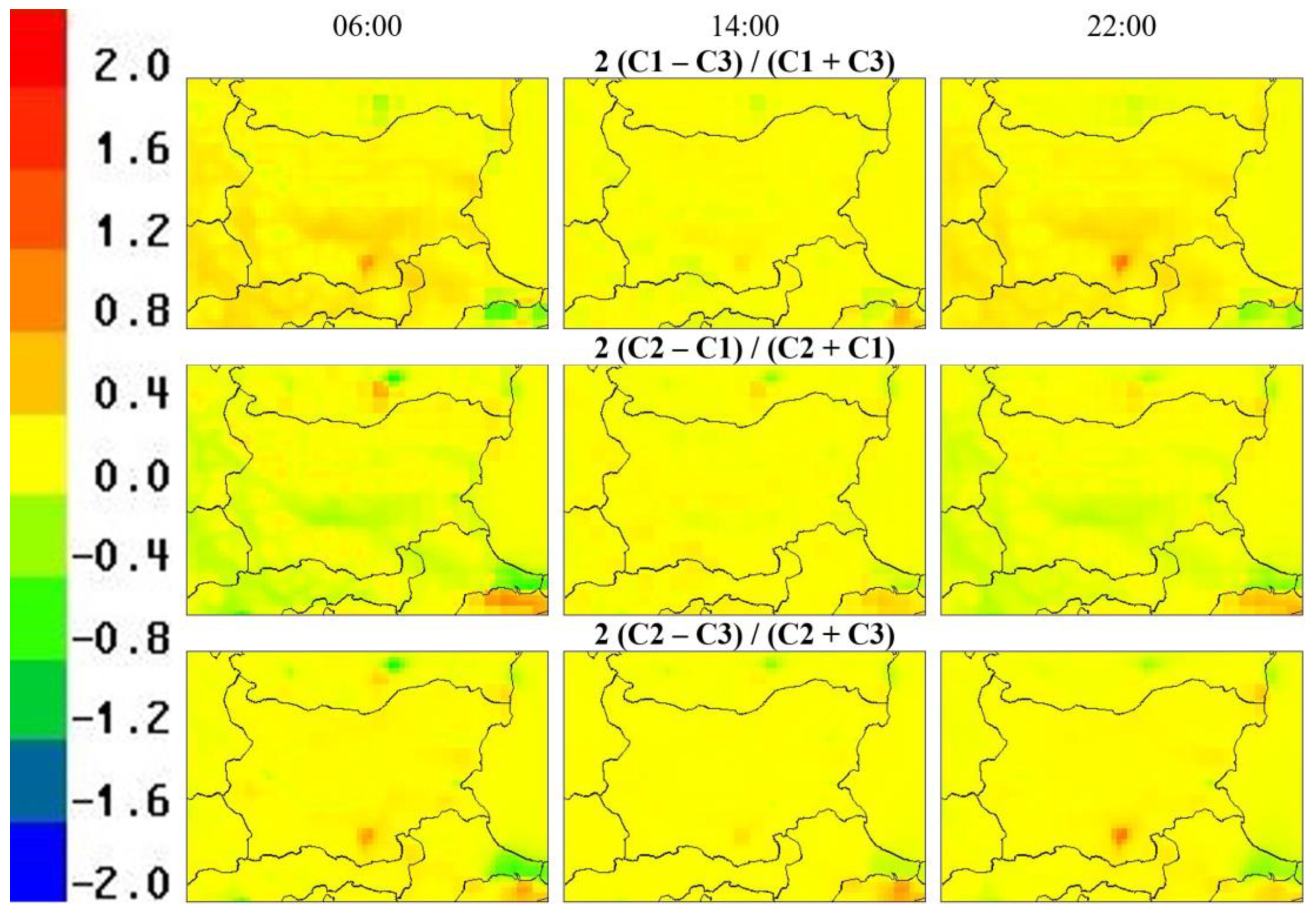
As should be expected, the relative differences for O3 (Figure 6) are much smaller and not explicitly related to pollution sources.
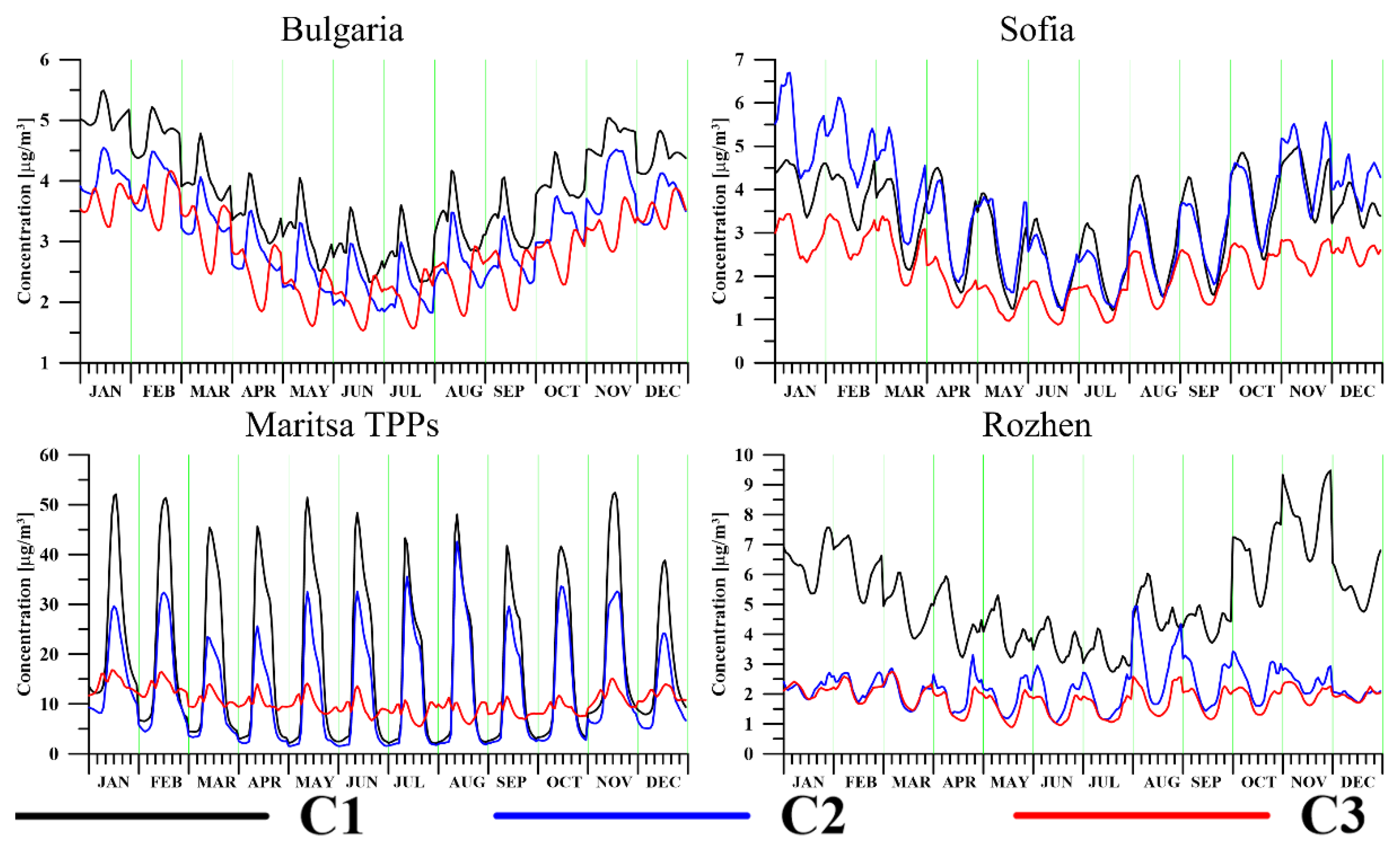
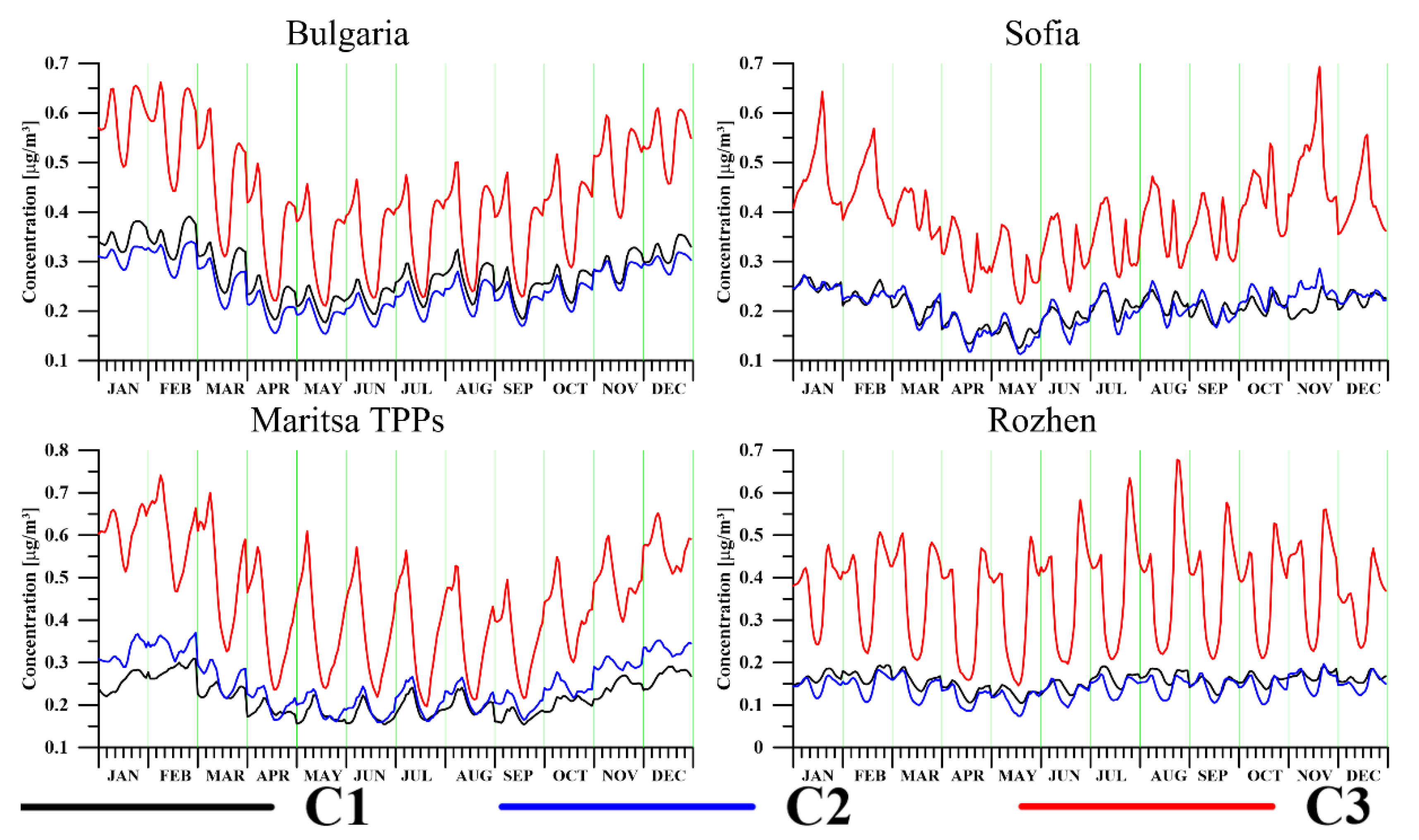
Diurnal and seasonal course averages over the ensemble surface concentrations of different pollutants for cases C1, C2, and C3 are shown in Figure 7, Figure 8 and Figure 9 for the city of Sofia, Maritsa TPPs, mountain point Rozhen (see Figure 1b) and averaged over Bulgaria.
On all the graphs for NO2 (Figure 7), the diurnal and seasonal course is well displayed. For Bulgaria, the curves for C1 and C2 overlap almost completely throughout the day, as well as for C3 during the day when the concentrations have minimums. The concentrations of NO2 at night for C3 for Bulgaria have maximum and are the highest compared to the other cases.
For Sofia, the C1 and C3 curves overlap completely, with the exception of the maximum concentrations in the afternoon in summer. This can be explained by the fact that Sofia is a large and rather homogeneous NO2 area source, so the source description resolution is not of much importance.
For Maritsa, TPPs C1 and C2 from November to February have the same course and close values. In the remaining months, there is a discrepancy in the phases of the minima and maxima in the average concentrations between these two simulations. From July to September, there was an overlap of the minimal values at noon of the average concentrations for all three cases. The average concentrations of C3 are the highest and in contra phase with the concentrations of C1 during the night. For Rozhen, it can be seen that during the winter C1 and C3 curves overlap almost all the time, but mostly in the afternoon when the average concentrations are again maximal, and in the other months, the overlap is at noon when the average concentrations are minimal and very close to those of C2. During the warm months, the concentrations of C3 are the highest, while those of C2 are the lowest throughout the year.
The average surface concentrations of SO2 (Figure 8) for all points also have a well-defined diurnal and seasonal course. As for Bulgaria, it can be seen that the average concentrations of the cases C1 and C2 are in contra phase with those of C3. For Sofia, there is no discrepancy between the minimums and the maximums for the different cases. It is interesting to note the period from November to May for Rozhen and Maritsa TPPs. For both points, the concentrations of the three cases have almost identical diurnal courses, while from July to October for Rozhen, the cases of C2 and C3 are in phase with those of C1. For Maritsa, TPPs C1 and C2 are in the contra phase with C3. On average for the country, C1 provides the highest average concentrations and C3 the lowest. For Sofia, from October to March, the average surface concentrations of C2 are the highest, and during the rest of the time, there is a slight dominance of the C1 with a more pronounced maximum in the evening during the summer. For Maritsa TPPs, the concentrations of C1 have the largest maximum values varying between 2–50 µg/m3, followed by C2 with values up to 35 µg/m3, while the variation of concentrations of C3 is in the range of 7–17 µg/m3. For Rozhen, the concentrations of C1 are the highest, and those of C2 and C3 are almost equal, those of C2 slightly higher.
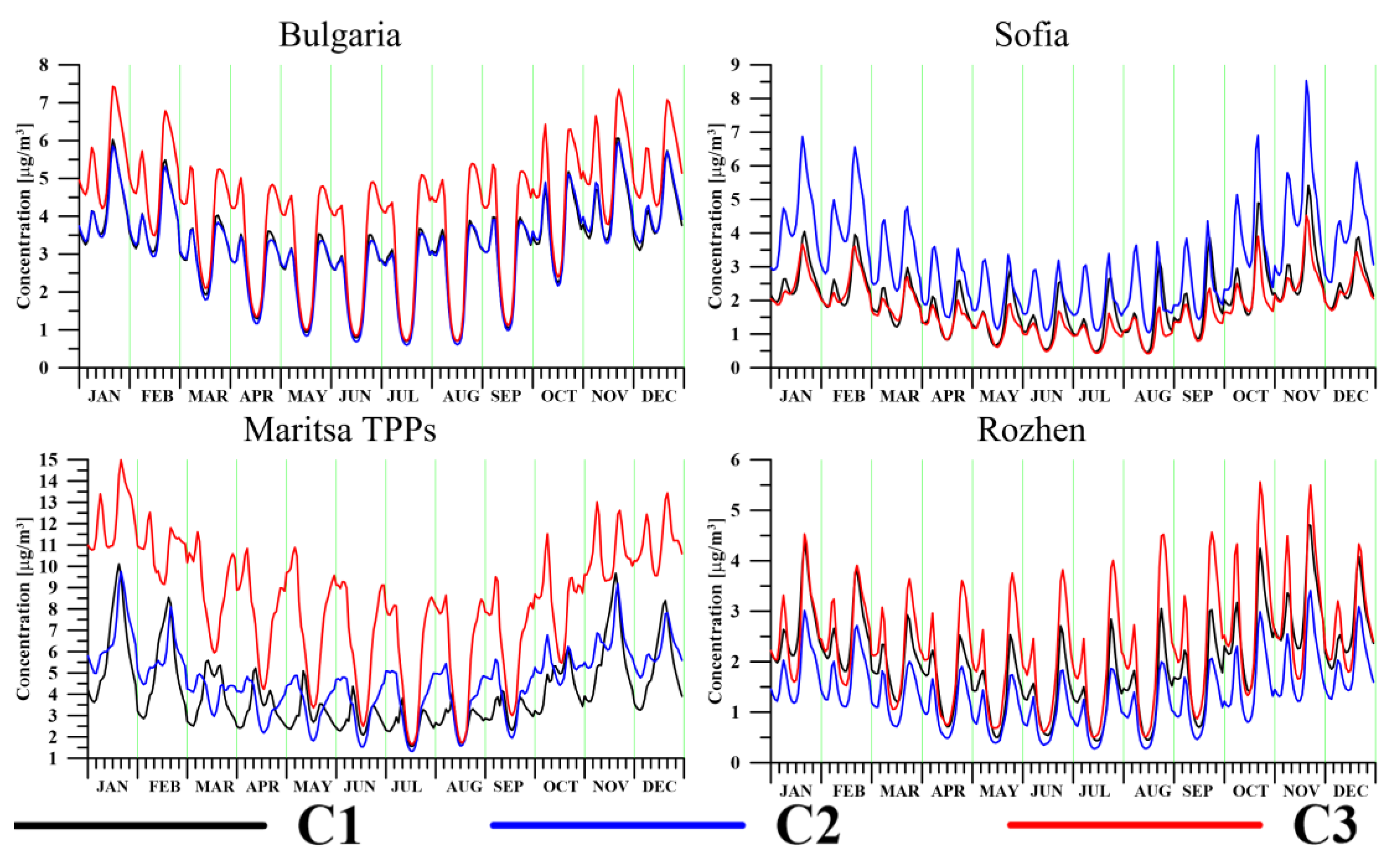
The four graphs for PM2.5 (Figure 9) show that the concentrations of C3 are the highest, and for all cases, the concentrations have a well-defined diurnal and seasonal course. For Bulgaria, the concentrations have a maximum in the cold half of the year and a minimum in the warm. Generally, for the country, C1 and C2 are almost identical, as the concentrations of C1 are slightly higher. For Sofia, the concentrations of C1 or C2 are also almost identical; only in November the concentrations of C2 are larger than C1 and in the contra phase. The average concentrations for Sofia show that the minimum for all three cases is in April and May, which could be due to the “washing” of the spring rains.
For Maritsa TPPs, the concentrations of C2 are slightly higher than C1 as for the three cases, the maximums are in the cold half of the year and the minimums in the warm half of the year, which is probably due to lower TPPs production and more intense turbulent transport in summer. For Rozhen, differences between C1 and C2 are observed only at noon (lower values of average concentrations), as the concentrations of C2 are slightly lower than those obtained from C1. For this point, the seasonal course of C1 and C2 is weak, yet lower values of winter and spring concentrations are slightly noticeable.
4. Discussion
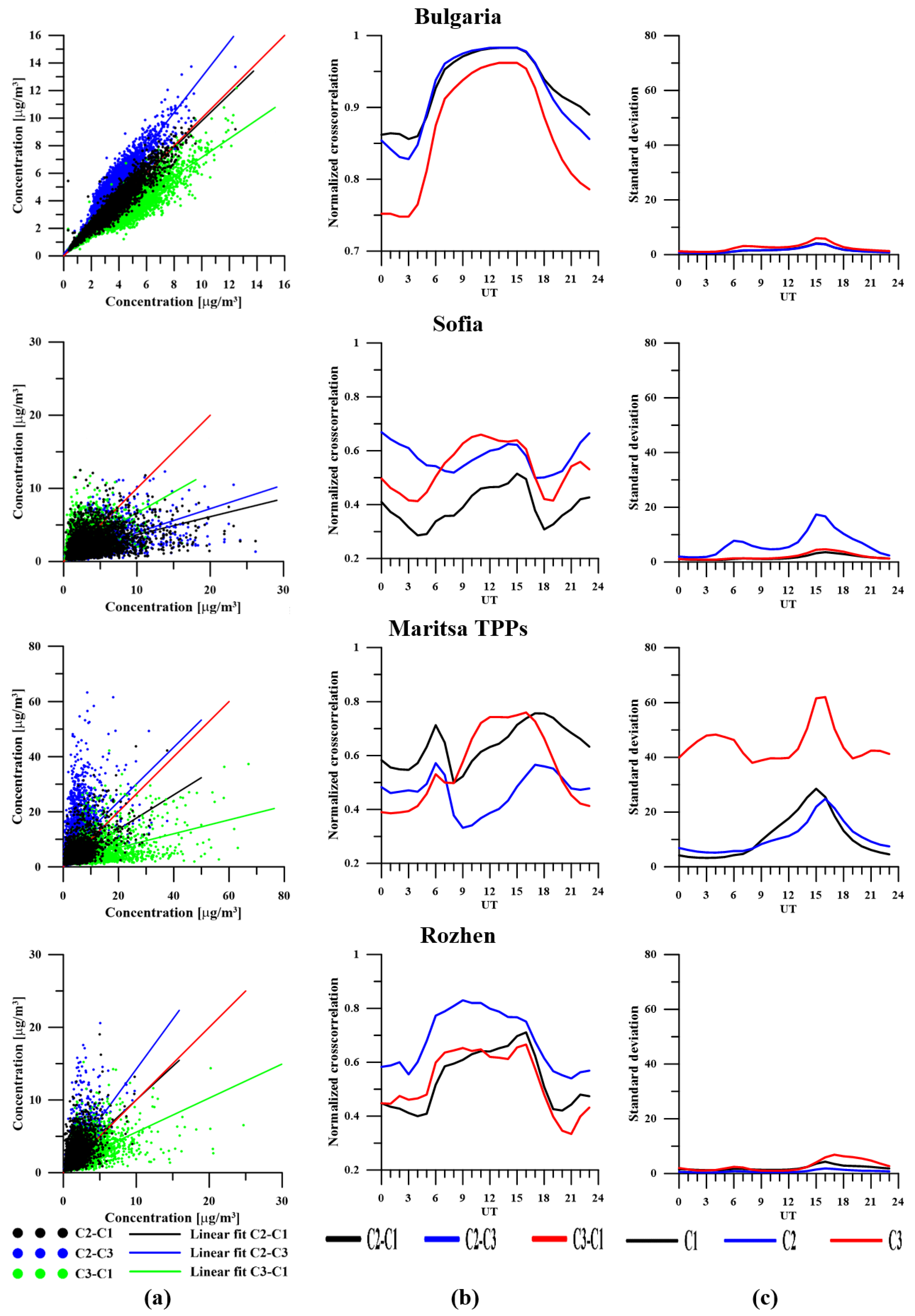
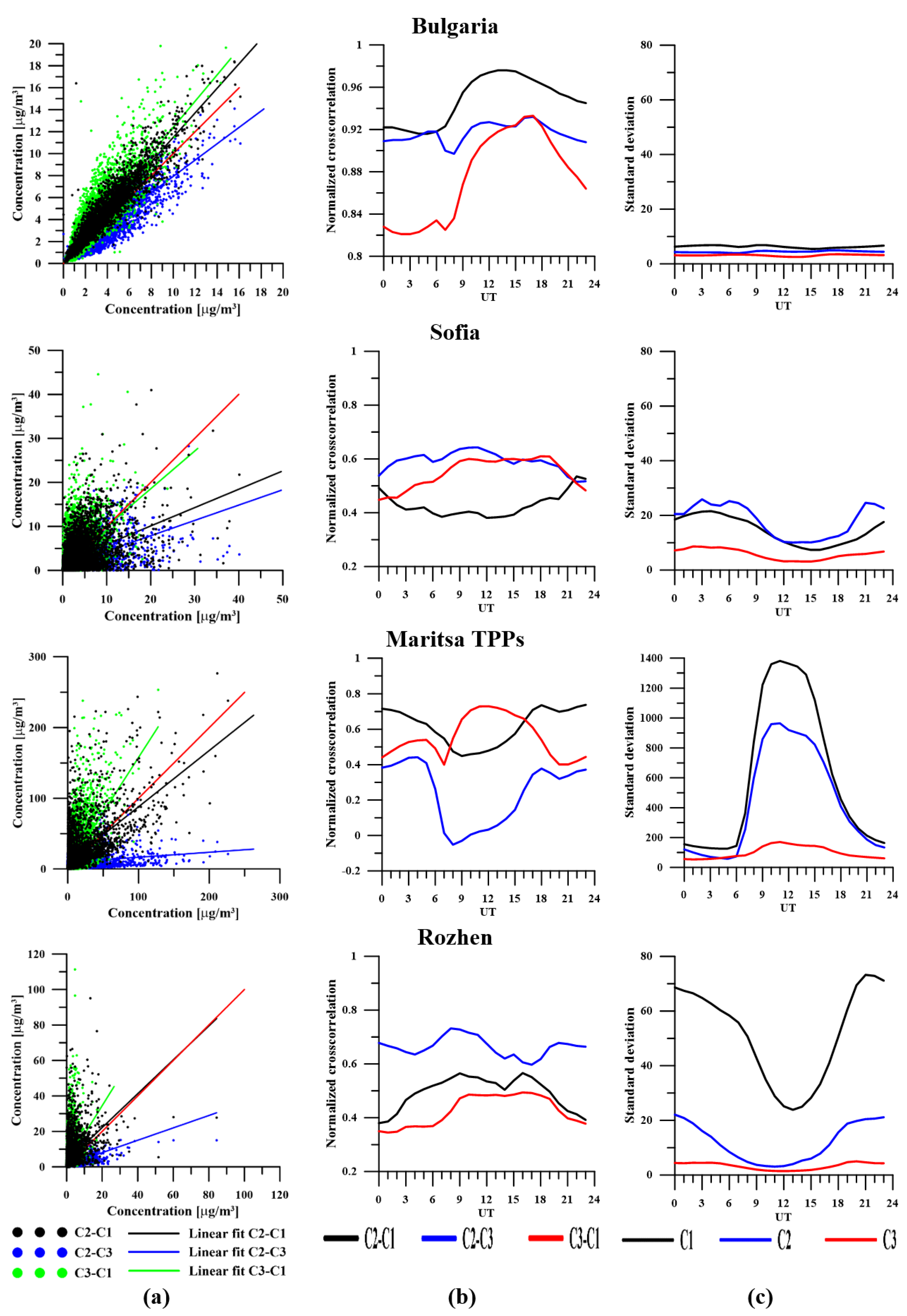
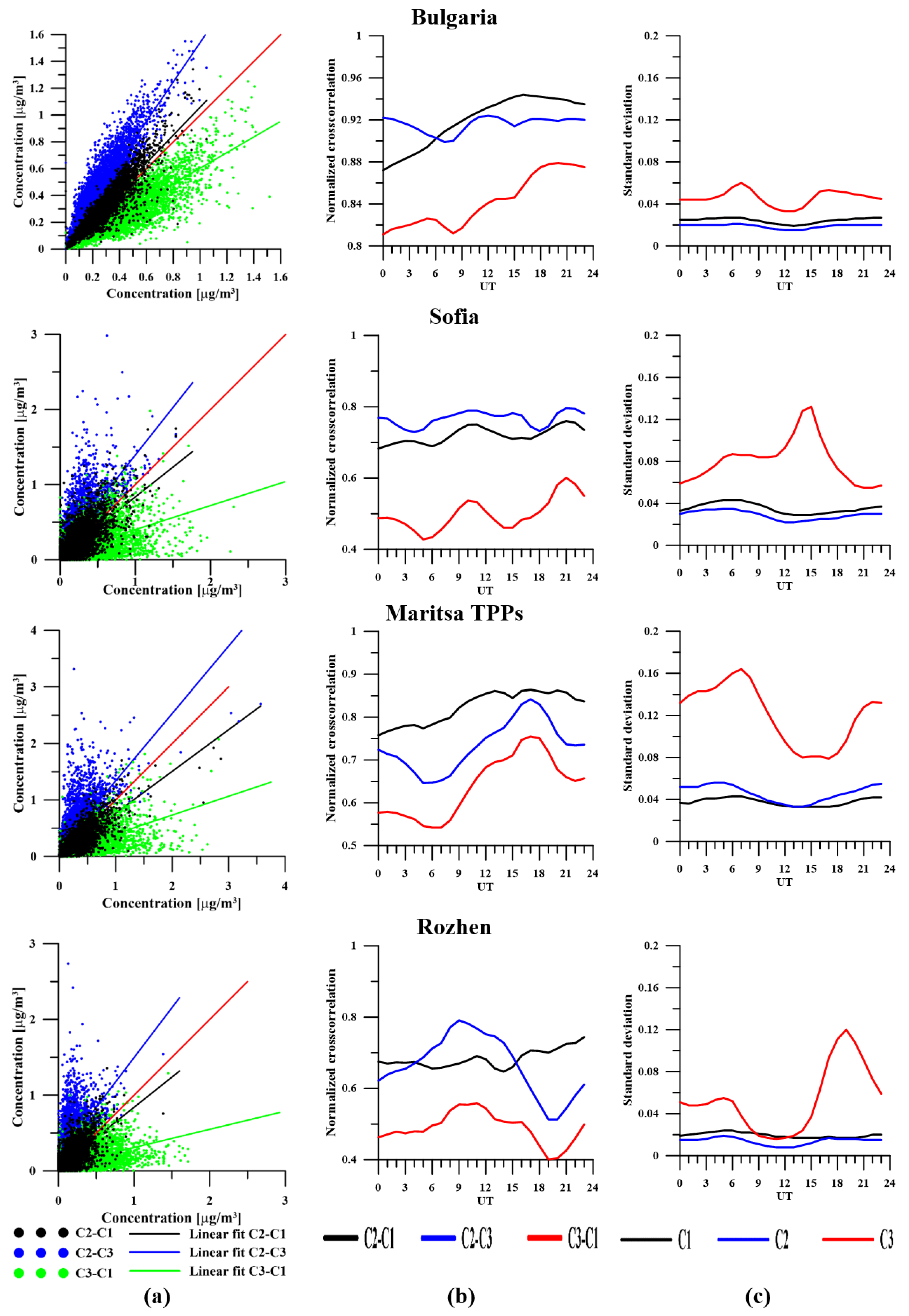
Figure 10, Figure 11 and Figure 12 show the comparisons of the regression and correlation dependences between the three cases, as well as the standard deviation of the hourly values of the concentrations of the NO2, SO2, and PM2.5 pollutants obtained under the three scenarios.
The left column of the figures (a) shows the linear regression between the values obtained at the same moments. The values of the first of the respective cases are located on the abscissa axis and on the ordinate of the second according to the legend. The red line shows the function y = x, and the colored lines show the linear regression between the cases obtained by the method of least squares. A match or proximity to the line y = x indicates, on average, the proximity of the values of the respective cases. Linear regressions with a larger slope show that the second case, on average, shows higher concentrations than the first, with a smaller slope—vice versa. The central column (b) shows the normalized cross-correlation between the concentrations centered by subtracting the mean at a certain time of day at zero time lag. Cross-correlations show the degree of similarity of the deviations from the mean values. The right-hand column (c) shows the standard deviation of the concentrations from their mean value for each hour of the day, which is a measure of the scattering of the concentration values around their mean values, shown in Figure 7, Figure 8 and Figure 9.
Concentrations calculated on average for the whole country show the highest correlations and the lowest standard deviations, which is obviously due to the averaging over a sufficiently wide region. The highest correlations (higher than 0.7) are observed between scenarios C2-C3 and C2-C1.
The NO2 concentrations at the individual points (Figure 10) show different regression and correlation dependencies. For Sofia, cases C1 and C3 show a significant decrease in values compared to C2, which can be seen from the regressions between them. Case C2 shows the highest scattering. In Maritsa TPPs, opposite results are obtained, the C2-C1 and C2-C3 regressions are close enough, and C3 shows the strongest scattering. The results for Rozhen are qualitatively and quantitatively close to the average for Bulgaria, which is obviously due to its remoteness from emission sources. For SO2 in Sofia, where there are no significant sources of this pollutant, there are practically no diurnal changes in the correlation, which has a low value of about 0.5. For Maritsa TPPs, large differences were observed between the behaviors of the concentrations in the three cases.
The regression C2-C3 is very small, and the correlation between them reaches zero at some hours. This corresponds to the abnormally low C3 means shown in Figure 8. The scatter ratio in the three cases corresponds to the ratios between the averages.
The diurnal course of the scattering at this point is with a maximum of around noon, unlike the other points for Bulgaria as an average. The diurnal course of the scattering for Rozhen is similar to that obtained for Sofia, but the standard deviations in Rozhen are significantly higher than those for Sofia and especially from the average for Bulgaria. The average concentrations for these sites shown in Figure 8 do not differ significantly.
The fine particulate matters PM2.5 have similar regression and correlation dependences both on average for Bulgaria and at specific points. The C2-C1 regression indicates an increase, C2-C3 is close to equivalence, and C2-C3 indicates a decrease. The correlation between C3 and C1 is the lowest for Bulgaria and all the selected points. Case C3 shows the highest scatter and also has the highest means, according to Figure 9.
For all the demonstrated compounds, the averaged over Bulgaria concentrations show a good fit and high correlation between C1 and C2 cases. The standard deviations for Bulgaria are also small. For the three selected points, the mutual behavior of cases C1, C2, and C3 is very different, largely depending on the emission source configuration.
5. Conclusions
The numerical experiments showed the significant impact of the grid resolution not only in the pollution concentration pattern but also in the demonstrated generalized characteristics. Averaged over a large territory (Bulgaria), however, the performance for cases C1 and C2 are quite similar.
Case C3, which is a kind of hybrid between cases C1 and C2, behaves strangely—it is not close to either of them. For Rozhen—a point distant from pollution sources, it correlates fairly well with C2. This probably is because, for the concentrations in points far from big sources, the resolution in the source description is not of much importance.
The above-demonstrated examples show that both the grid and the source description resolution play their role in the atmospheric composition formation—in different ways and to different extents, depending on the location and the specific pollutant. The grid resolution influences the atmospheric dynamics, the accuracy of the numerical solutions, and the chemical transformation rates. The experiments and the analysis performed do not suggest the idea of how these three factors interact to jointly form the atmospheric composition. Maybe applying the “Integrated process analysis” procedure of the CMAQ model can provide some clues in this direction. This could be a task for future work.
Author Contributions
Conceptualization, K.G. and G.G.; methodology, K.G., G.G. and P.M.; software, K.G., G.G. and P.M.; formal analysis, K.G., G.G. and P.M.; investigation, K.G.; resources, G.G.; data curation, G.G.; writing—original draft preparation, K.G., G.G. and P.M.; writing—review and editing, K.G. and G.G.; visualization, G.G. and P.M.; supervision, K.G. and G.G.; project administration, K.G. and G.G.; funding acquisition, G.G. All authors have read and agreed to the published version of the manuscript.
Funding
This work has been carried out in the framework of the National Science Program “Environmental Protection and Reduction of Risks of Adverse Events and Natural Disasters”, approved by the Resolution of the Council of Ministers № 577/17.08.2018 and supported by the Ministry of Education and Science (MES) of Bulgaria (Agreement № D01-279/03.12.2021). This work has also been accomplished with the financial support of Grant No BG05M2OP001-1.001-0003, financed by the Science and Education for Smart Growth Operational Program (2014-2020) and co-financed by the European Union through the European Structural and Investment funds.
Institutional Review Board Statement
Not applicable.
Informed Consent Statement
Not applicable.
Data Availability Statement
Not applicable.
Acknowledgments
Special thanks are due to US EPA and US NCEP for providing free-of-charge data and software and to the Netherlands Organization for Applied Scientific research (TNO) for providing the high resolution European anthropogenic emission inventory.
Conflicts of Interest
The authors declare no conflict of interest.
References
- Fisher, B.E.A.; Kukkonen, J.; Schatzmann, M. Meteorology applied to urban air pollution problems COST 715. Int. J. Environ. Pollut. 2001, 16, 560–570. [Google Scholar] [CrossRef]
- Fisher, B.; Joffre, S.; Kukkonen, J.; Piringer, M.; Rotach, M.; Schatzmann, M. Meteorology applied to urban air pollution problems. In Final Report COST-715 Action; Demetra Ltd. Publisher: Sofia, Bulgaria, 2005; p. 276. [Google Scholar]
- Fisher, B.; Kukkonen, J.; Piringer, M.; Rotach, M.W.; Schatzmann, M. Meteorology applied to urban air pollution problems: Concepts from COST 715. Atmos. Chem. Phys. 2006, 6, 555–564. [Google Scholar] [CrossRef] [Green Version]
- Kukkonen, J.; Pohjola, M.; Sokhi, R.S.; Luhana, L.; Kitwiroon, N.; Rantamäki, M.; Berge, E.; Odegaard, V.; Slørdal, L.H.; Denby, B.; et al. Analysis and evaluation of selected local-scale PM10 air pollution episodes in four European cities: Helsinki, London, Milan and Oslo. Atmos. Environ. 2005, 39, 2759–2773. [Google Scholar] [CrossRef]
- Kukkonen, J.; Sokhi, R.S.; Slordal, L.H.; Finardi, S.; Fay, B.; Millan, M.; Salvador, R.; Palau, J.L.; Rasmussen, A.; Schayes, G.; et al. Analysis and evaluation of European air pollution episodes, in: Meteorology applied to urban air pollution 3720 problems. In Final Report COST Action 715; Fisher, B., Ed.; Demetra Ltd. Publisher: Sofia, Bulgaria, 2005; pp. 99–114. [Google Scholar]
- McNider, R.T.; Pour-Biazar, A. Meteorological modeling relevant to mesoscale and regional air quality applications: A review. J. Air Waste Manag. 2020, 70, 2–43. [Google Scholar] [CrossRef] [PubMed]
- Rao, S.T.; Luo, H.; Astitha, M.; Hogrefe, C.; Garcia, V.; Mathur, R. On the limit to the accuracy of regional-scale air quality models. Atmos. Chem. Phys. 2020, 20, 1627–1639. [Google Scholar] [CrossRef] [PubMed] [Green Version]
- Parra, R. Effects of global meteorological datasets in modeling meteorology and air quality in the andean region of southern Ecuador. In Proceedings of the 12th International Conference on Air Quality, Science and Application, Online, 9–13 March 2020. [Google Scholar]
- Gilliam, R.C.; Hogrefe, C.; Godowitch, J.M.; Napelenok, S.; Mathur, R.; Rao, S.T. Impact of inherent meteorology uncertainty on air quality model predictions. J. Geophys. Res.-Atmos. 2015, 120, 12259–12280. [Google Scholar] [CrossRef]
- Baklanov, A.; Brunner, D.; Carmichael, G.; Flemming, G.; Freitas, S.; Gauss, M.; Hov, Ø.; Mathur, R.; Schlünzen, H.; Seigneur, C.; et al. Key Issues for Seamless Integrated Chemistry–Meteorology Modeling. BAMS 2017, 98, 2285–2292. [Google Scholar] [CrossRef]
- Baklanov, A.; Zhang, Y. Advances in air quality modeling and forecasting. Glob. Transit. 2020, 2, 261–270. [Google Scholar] [CrossRef]
- Baklanov, A.; .Schlünzen, K.; Suppan, P.; Baldasano, J.; Brunner, D.; Aksoyoglu, S.; Carmichael, G.; Douros, J.; Flemming, J.; Forkel, R.; et al. Online coupled regional meteorology chemistry models in Europe: Current status and prospects. Atmos. Chem. Phys. 2014, 14, 317–398. [Google Scholar] [CrossRef] [Green Version]
- Matthias, V.; Arndt, J.A.; Aulinger, A.; Bieser, J.; van der Denier Gon, H.; Kranenburg, R.; Kuenen, J.; Neumann, D.; Pouliot, G.; Quante, M. Modeling emissions for three-dimensional atmospheric chemistry transport models. J. Air Waste Manag. 2018, 68, 763–800. [Google Scholar] [CrossRef]
- EMEP/EEA. Chapter 7: Spatial mapping of emissions. In EMEP/EEA Air Pollutant Emission Inventory Guidebook 2019: Technical Guidance to Prepare National Emission Inventories; No 13/2019; Publications Office of the European Union: Luxembourg, 2019. [Google Scholar]
- Arunachalam, S.; Holland, A.; Do, B.; Abraczinskas, M. A quantitative assessment of the influence of grid resolution on predictions of future-year air quality in North Carolina, USA. Atmos. Environ. 2006, 40, 5010–5025. [Google Scholar] [CrossRef]
- Arunachalam, S.; Wang, B.; Davis, N.; Baek, B.H.; Levy, J.I. Effect of chemistry-transport model scale and resolution on population exposure to PM2.5 from aircraft emissions during landing and takeoff. Atmos. Environ. 2011, 45, 3294–3300. [Google Scholar] [CrossRef]
- Cohan, D.S.; Hu, Y.; Russel, A.G. Dependence of ozone sensitivity analysis on grid resolution. Atmos. Environ. 2006, 40, 126–135. [Google Scholar] [CrossRef]
- Fountoukis, C.; Koraj, D.H.; Denier van der Gon, H.A.C.; Charalampidis, P.E.; Pilinis, C.; Pandis, S.N. Impact of grid resolution on the predicted fine PM by a regional 3-D chemical transport model. Atmos. Environ. 2013, 68, 24–32. [Google Scholar] [CrossRef]
- Gao, X.; Xu, Y.; Zhao, Z.; Pal, J.; Giorgi, F. On the role of resolution and topography in the simulation of East Asia precipitation. Theor. Appl. Climatol. 2006, 86, 173–185. [Google Scholar] [CrossRef]
- Gillani, N.V.; Pleim, J.E. Sub-grid-scale features of anthropogenic emissions of NOx and VOC in the context of regional eulerian models. Atmos. Environ. 1996, 30, 2043–2059. [Google Scholar] [CrossRef]
- Hodnebrog, Ø.; Stordal, F.; Berntsen, T.K. Does the resolution of megacity emissions impact large scale ozone? Atmos. Environ. 2011, 45, 6852–6862. [Google Scholar] [CrossRef] [Green Version]
- Jang, J.C.; Jeffries, H.E.; Byun, D.; Pleim, J.E. Sensitivity of ozone to model grid resolution—I. Application of high-resolution regional acid deposition model. Atmos. Environ. 1995, 29, 3085–3100. [Google Scholar] [CrossRef]
- Jang, J.C.; Jeffries, H.E.; Tonnesen, S. Sensitivity of ozone to model grid resolution—II. Detailed process analysis for ozone chemistry. Atmos. Environ. 1995, 29, 3101–3114. [Google Scholar] [CrossRef]
- Jimenez, P.; Jorba, O.; Parra, R.; Baldasano, J.M. Evaluation of MM5-EMICAT2000-CMAQ performance and sensitivity in complex terrain: High-resolution application to the northeastern Iberian Peninsula. Atmos. Environ. 2006, 40, 5056–5072. [Google Scholar] [CrossRef]
- Kuik, F.; Lauer, A.; Churkina, G.; Denier van der Gon, H.A.C.; Fenner, D.; Mar, K.A.; Butler, T.M. Air quality modelling in the Berlin-Brandenburg Region using WRF-Chem v3.7.1: Sensitivity to resolution of model grid and input data. Geosci. Model Dev. 2016, 9, 4339–4363. [Google Scholar] [CrossRef] [Green Version]
- Kumar, N.; Russel, A.G. Multiscale air quality modeling of the Northeastern United States. Atmos. Environ. 1996, 30, 1099–1116. [Google Scholar] [CrossRef]
- Lauwaet, D.; Viaene, P.; Brisson, E.; van Noije, T.; Strunk, A.; Van Looy, S.; Maiheu, B.; Veldeman, N.; Blyth, L.; De Ridder, K.; et al. Impact of nesting resolution jump on dynamical downscaling ozone concentrations over Belgium. Atmos. Environ. 2013, 67, 46–52. [Google Scholar] [CrossRef]
- Leung, L.R.; Qian, Y. The sensitivity of precipitation and snowpack simulations to model resolution via nesting in regions of complex terrain. J. Hydrometeorol. 2003, 4, 1025–1043. [Google Scholar] [CrossRef]
- Li, Y.; Henze, D.K.; Jack, D.; Kinney, P.L. The influence of air quality model resolution on health impact assessment for fine particulate matter and its components. Air Qual. Atmos. Health 2015, 9, 51–68. [Google Scholar] [CrossRef] [Green Version]
- Mass, C.F.; Ovens, D.; Westrick, K. Does increasing horizontal resolution produce more skillful forecasts? The results of two years of real-time numerical weather prediction over the Pacific Northwest. Bull. Am. Meteorol. Soc. 2002, 83, 407. [Google Scholar] [CrossRef]
- Menut, L.; Coll, I.; Cautenet, S. Impact of meteorological data resolution on the forecasted ozone concentrations during the ESCOMPTE IOP2a and IOP2b. Atmos. Res. 2005, 74, 139–159. [Google Scholar] [CrossRef]
- Mensink, C.; De Ridder, K.; Deutsch, F.; Lefebre, F.; Van de Vel, K. Examples of scale interactions in local, urban, and regional air quality modelling. Atmos. Res. 2008, 89, 351–357. [Google Scholar] [CrossRef]
- Micea, M.; Cappelletti, A.; Briganti, G.; Vitali, L.; Pace, G.; Marri, P.; Silibello, C.; Finardi, S.; Calori, G.; Zanini, G. Impact of horizontal grid resolution on air quality modeling: A case study over Italy. In Proceedings of the 13th Conference on Harmonisation within Atmospheric Dispersion Modelling for Regulatory Purposes, Paris, France, 1–4 June 2010; pp. 166–170. [Google Scholar]
- Palau, J.; Pérez-Landa, G.; Diéguez, J.; Monter, C.; Millán, M. The importance of meteorological scales to forecast air pollution scenarios on coastal complex terrain. Atmos. Chem. Phys. 2005, 5, 2771–2785. [Google Scholar] [CrossRef] [Green Version]
- Pan, S.; Choi, Y.; Roy, A.; Jeon, W. Allocating emissions to 4 km and 1 km horizontal spatial resolutions and its impact on simulated NOx and O3 in Houstin, TX. Atmos. Environ. 2017, 164, 398–415. [Google Scholar] [CrossRef]
- Punger, E.M.; West, J.J. The effect of grid resolution on estimates of the burden of ozone and fine particulate matter on premature mortality in the United States. Air Quality. Atmos. Health 2013, 6, 563–573. [Google Scholar] [CrossRef] [PubMed]
- Queen, A.; Zhang, Y. Examining the sensitivity of MM5-CMAQ predictions to explicit microphysics schemes and horizontal grid resolutions, Part III–The impact of horizontal grid resolution. Atmos. Environ. 2008, 42, 3869–3881. [Google Scholar] [CrossRef]
- Schaap, M.; Cuvelier, C.; Hendriks, C.; Bessagnet, B.; Baldasano, J.M.; Colette, A.; Thunis, P.; Karam, D.; Fagerli, H.; Graff, A.; et al. Performance of European chemistry transport models as function of horizontal resolution. Atmos. Environ. 2015, 112, 90–105. [Google Scholar] [CrossRef] [Green Version]
- Stroud, C.A.; Makar, P.A.; Moran, M.D.; Gong, W.; Gong, S.; Zhang, J.; Hayden, K.; Mihele, C.; Brook, J.R.; Abbarr, J.P.D.; et al. Impact of model grid spacing on regional- and urban- scale air quality predictions of organic aerosol. Atmos. Chem. Phys. 2011, 11, 3107–3118. [Google Scholar] [CrossRef] [Green Version]
- Tan, J.; Zhang, Y.; Ma, W.; Yu, Q.; Wang, J.; Chen, L. Impact of spatial resolution on air quality simulation: A case study in highly industrial area in Shanghai, China. Atmos. Pollut. Res. 2015, 6, 322–333. [Google Scholar] [CrossRef] [Green Version]
- Thompson, T.M.; Selin, N.E. Influence of air quality model resolution on uncertainty assocaited with health impacts. Atmos. Chem. Phys. 2012, 12, 9753–9762. [Google Scholar] [CrossRef] [Green Version]
- Thompson, T.M.; Saari, R.K.; Selin, N.E. Air quality resolution for health impacts assessment: Influence of regional characteristics. Atmos. Chem. Phys. 2014, 14, 969–978. [Google Scholar] [CrossRef] [Green Version]
- Tie, X.; Brasseur, G.; Ying, Z. Impact of model resolution on chemical ozone formation in Mexico City: Application of the WRF-Chem model. Atmos. Chem. Phys. 2010, 10, 8983–8995. [Google Scholar] [CrossRef] [Green Version]
- Valarie, M.; Menut, L. Does an increase in air quality models’ resolution bring surface ozone concentrations closer to reality? J. Atmos. Ocean. Technol. 2008, 25, 1955–1968. [Google Scholar] [CrossRef]
- Wolke, R.; Schröder, W.; Schrödner, R.; Eberhard, R. Influence of grid resolution and meteorological forcing on simulated European air quality: A sensitivity study with the modeling system COSMO-MUSCAT. Atmos. Environ. 2012, 53, 110–130. [Google Scholar] [CrossRef]
- Fillingham, M. The Influence of CMAQ Model Resolution on Predicted Air Quality and Associated Health Impacts. Master’s Thesis, Carleton University, Ottawa, ON, Canada, 2019. [Google Scholar]
- Skamarock, W.C.; Klemp, J.B.; Dudhia, J.; Gill, D.O.; Barker, D.M.; Wang, W.; Powers, J.G. A Description of the Advanced Research Wrf Version 2; National Center for Atmospheric Research Boulder Co Mesoscale and Microscale Meteorology Div: Boulder, CO, USA, 2007. [Google Scholar]
- Byun, D.; Ching, J. Science Algorithms of the EPA Models-3 Community Multiscale Air Quality (CMAQ) Modeling System; EPA Report; 600/R-99/030; EPA: Washington, DC, USA, 1999. [Google Scholar]
- Byun, D.; Schere, K.L. Review of the governing equations, computational algorithms, and other components of the models-3 community multiscale air quality (CMAQ) modeling system. Appl. Mech. 2006, 59, 51–76. [Google Scholar] [CrossRef]
- CEP. Sparse Matrix Operator Kernel Emission (SMOKE) Modeling System; University of Carolina, Carolina Environmental Programs, Research Triangle Park: Chapel Hill, NC, USA, 2003. [Google Scholar]
- Gadzhev, G.; Ganev, K.; Miloshev, N. Numerical study of the atmospheric composition climate of Bulgaria-Validation of the computer simulation results. Int. J. Environ. Pollut. 2015, 57, 189–201. [Google Scholar] [CrossRef]
- Georgieva, I.; Ivanov, V. Air Quality Index Evaluations for Sofia city. In Proceedings of the 17th IEEE International Conference on Smart Technologies, IEEE EUROCON 2017, Ohrid, North Macedonia, 6–8 July 2017. [Google Scholar]
- Georgieva, I.; Ivanov, V. Impact of the air pollution on the quality of life and health risks in Bulgaria. In Proceedings of the HARMO 2017—18th International Conference on Harmonisation within Atmospheric Dispersion Modelling for Regulatory Purposes, Bologna, Italy, 9–12 October 2017. [Google Scholar]
- Georgieva, I.; Ivanov, V. Computer Simulations Of The Impact Of Air Pollution On The Quality Of Life And Health Risks In Bulgaria. Int. J. Environ. Pollut. 2018, 64, 35–46. [Google Scholar] [CrossRef]
- Georgieva, I.; Miloshev, N. Computer Simulations of PM Concentrations Climate for Bulgaria. In Proceedings of the International Conference on “Numerical Methods for Scientific Computations and Advanced Applications” (NMSCAA’18), Hissarya, Bulgaria, 28–31 May 2018; pp. 46–49. [Google Scholar]
- Georgieva, I. Air Pollution Assessment for Sofia City—Dominant Pollutants Recurrence Which Determines the air Quality Status. In Proceedings of the 11th Congress of the Balkan Geophysical Society, Bucharest, Romania, 10–14 October 2021; Volume 2021. [Google Scholar]
- Ivanov, V.; Georgieva, I. Basic Facts about Numerical Simulations of Atmospheric Composition in the City of Sofia. Atmosphere 2021, 12, 1450. [Google Scholar] [CrossRef]
- Visschedijk, A.; Zandveld, P.; van der Gon, H. A High Resolution Gridded European Emission Database for the EU Integrated Project GEMS; TNO report 2007-A-R0233/B; TNO: Apeldoorn, The Netherlands, 2007. [Google Scholar]
- Builtjes, P.J.H.; van Loon, M.; Schaap, M.; Teeuwisse, S.; Visschedijk, A.J.H.; Bloos, J.P. Project on the Modelling and Verification of Ozone Reduction Strategies: Contribution of TNO-MEP; TNO-report, MEP-R2003/166; TNO: Apeldoorn, The Netherlands, 2003. [Google Scholar]
- Schaap, M.; Timmermans, R.M.A.; Roemer, M.; Boersen, G.A.C.; Builtjes, P.J.H.; Sauter, F.J.; Velders, G.J.M.; Beck, J.P. The LOTOS–EUROS model: Description, validation and latest developments. Int. J. Environ. Pollut. 2008, 32, 270–290. [Google Scholar] [CrossRef]
- Gery, M.W.; Whitten, G.Z.; Killus, J.P.; Dodge, M.C. A Photochemical Kinetics Mechanism for Urban and Regional Scale Computer Modeling. J. Geophys. Res. 1989, 94, 12925–12956. [Google Scholar] [CrossRef]
- Ryan, R. Memorandum: Speciation Profiles and Assignment Files Located on EMCH, US EPA Emission Factor and Inventory Group. Available online: https://www3.epa.gov/ttn/chief/old/emch/speciation/emch_speciation_profile.doc (accessed on 19 April 2022).
- Gadzhev, G.; Ganev, K.; Miloshev, N.; Syrakov, D.; Prodanova, M. Numerical Study of the Atmospheric Composition in Bulgaria. Comput. Math. Appl. 2013, 65, 402–422. [Google Scholar] [CrossRef]
- Guenther, A.; Geron, C.; Pierce, T.; Lamb, B.; Harley, P.; Fall, R. Natural Emissions of Non-Methane Volatile Organic Compounds, Carbon Monoxide, and Oxides of Nitrogen From North America. Atmos. Environ. 2000, 34, 2205–2230. [Google Scholar] [CrossRef] [Green Version]
- Pierce, T.; Geron, C.; Bender, L.; Dennis, R.; Tennyson, G.; Guenther, A. The Influence of Increased Isoprene Emissions on Regional Ozone Modeling. J. Geophys. Res. 1998, 103, 25611–25629. [Google Scholar] [CrossRef] [Green Version]
- Schwede, D.; Pouliot, G.; Pierce, T. Changes to the Biogenic Emissions Invenory System Version 3 (BEIS3). In Proceedings of the 4th CMAS Models-3 Users’ Conference, Chapel Hill, NC, USA, 26–28 September 2005. [Google Scholar]
Figure 1.
(a) The three nested integration domains with horizontal grid resolution 81 km (D1), 27 km (D2) and 9 km (D3), (b) Topography map of Bulgaria with the points Sofia (1), Maritsa TPPs (2) and Rozhen (3).
Figure 1.
(a) The three nested integration domains with horizontal grid resolution 81 km (D1), 27 km (D2) and 9 km (D3), (b) Topography map of Bulgaria with the points Sofia (1), Maritsa TPPs (2) and Rozhen (3).


Figure 2.
Annually averaged surface concentrations of NO2 [µg/m3] for cases C1, C2 and C3.

Figure 3.
Annually averaged relative differences of the surface concentrations of NO2 between cases C1 and C3, C2 and C1, C2 and C3 respectively.
Figure 3.
Annually averaged relative differences of the surface concentrations of NO2 between cases C1 and C3, C2 and C1, C2 and C3 respectively.

Figure 4.
Annually averaged relative differences of the surface concentrations of SO2 between cases C1 and C3, C2 and C1, C2 and C3 respectively.
Figure 4.
Annually averaged relative differences of the surface concentrations of SO2 between cases C1 and C3, C2 and C1, C2 and C3 respectively.

Figure 5.
Annually averaged relative differences of the surface concentrations of PM2.5 between cases C1 and C3, C2 and C1, C2 and C3 respectively.
Figure 5.
Annually averaged relative differences of the surface concentrations of PM2.5 between cases C1 and C3, C2 and C1, C2 and C3 respectively.

Figure 6.
Annually averaged relative differences of the surface concentrations of O3 between cases C1 and C3, C2 and C1, C2 and C3 respectively.
Figure 6.
Annually averaged relative differences of the surface concentrations of O3 between cases C1 and C3, C2 and C1, C2 and C3 respectively.

Figure 7.
Diurnal and seasonal course of averaged over the ensemble surface concentrations of NO2 [µg/m3] for cases C1, C2 and C3.
Figure 7.
Diurnal and seasonal course of averaged over the ensemble surface concentrations of NO2 [µg/m3] for cases C1, C2 and C3.

Figure 8.
Diurnal and seasonal course of averaged over the ensemble surface concentrations of SO2 [µg/m3] for cases C1, C2 and C3.
Figure 8.
Diurnal and seasonal course of averaged over the ensemble surface concentrations of SO2 [µg/m3] for cases C1, C2 and C3.

Figure 9.
Diurnal and seasonal course of averaged over the ensemble surface concentrations of PM2.5 [µg/m3] for cases C1, C2 and C3.
Figure 9.
Diurnal and seasonal course of averaged over the ensemble surface concentrations of PM2.5 [µg/m3] for cases C1, C2 and C3.

Figure 10.
Comparisons of the regression (a) and correlations (b) and standard deviation (c) for NO2 for the three cases.
Figure 10.
Comparisons of the regression (a) and correlations (b) and standard deviation (c) for NO2 for the three cases.

Figure 11.
Comparisons of the regression (a) and correlations (b) and standard deviation (c) for SO2 for the three cases.
Figure 11.
Comparisons of the regression (a) and correlations (b) and standard deviation (c) for SO2 for the three cases.

Figure 12.
Comparisons of the regression (a) and correlations (b) and standard deviation (c) for PM2.5 for the three cases.
Figure 12.
Comparisons of the regression (a) and correlations (b) and standard deviation (c) for PM2.5 for the three cases.

Publisher’s Note: MDPI stays neutral with regard to jurisdictional claims in published maps and institutional affiliations. |
© 2022 by the authors. Licensee MDPI, Basel, Switzerland. This article is an open access article distributed under the terms and conditions of the Creative Commons Attribution (CC BY) license (https://creativecommons.org/licenses/by/4.0/).
Share and Cite
MDPI and ACS Style
Gadzhev, G.; Ganev, K.; Mukhtarov, P. Influence of the Grid Resolutions on the Computer-Simulated Surface Air Pollution Concentrations in Bulgaria. Atmosphere 2022, 13, 774. https://doi.org/10.3390/atmos13050774
AMA Style
Gadzhev G, Ganev K, Mukhtarov P. Influence of the Grid Resolutions on the Computer-Simulated Surface Air Pollution Concentrations in Bulgaria. Atmosphere. 2022; 13(5):774. https://doi.org/10.3390/atmos13050774
Chicago/Turabian StyleGadzhev, Georgi, Kostadin Ganev, and Plamen Mukhtarov. 2022. "Influence of the Grid Resolutions on the Computer-Simulated Surface Air Pollution Concentrations in Bulgaria" Atmosphere 13, no. 5: 774. https://doi.org/10.3390/atmos13050774
Note that from the first issue of 2016, this journal uses article numbers instead of page numbers. See further details here.