
Revisiting the Contrasting Response of Polar Stratosphere to the Eastern and Central Pacific El Niños


Faculty of Geography, Moscow State University (MSU), Moscow 119991, Russia
*
Authors to whom correspondence should be addressed.
Atmosphere 2022, 13(5), 682; https://doi.org/10.3390/atmos13050682
Submission received: 16 February 2022
/
Revised: 8 April 2022
/
Accepted: 15 April 2022
/
Published: 24 April 2022
(This article belongs to the Special Issue ENSO Atmospheric Teleconnections to the Mid-to-High Latitudes)
Abstract
:El Niño Southern Oscillation (ENSO) invokes the release of a large amount of heat and moisture into the tropical atmosphere, inducing circulation anomalies. The circulation response to ENSO propagates both horizontally poleward and vertically into the stratosphere. Here, we investigate the remote response of the polar stratosphere to ENSO using reanalysis data, along with composite and regression analysis. In particular, we focus on inter-event variability resulting from two ENSO types (the Eastern Pacific (EP) and the Central Pacific (CP) El Niño) and the inter-hemispheric difference in the ENSO responses. Consistent with previous results, we show that ENSO is associated with a weakening in the stratospheric polar vortex but emphasize that the polar stratosphere response strongly depends on the ENSO types, differs between the hemispheres, and changes from the lower to middle stratosphere. The main inter-hemispheric asymmetry manifests in response to the EP El Niño, which is not significant in the Southern Hemisphere, while CP events are associated with pronounced weakening in the polar vortex in both hemispheres. The weakening in the stratospheric polar vortex arguably results from the intensification in the wave flux from the troposphere into the stratosphere and is accompanied by increased heat transport. The latter causes stratospheric warming in the Artic and Antarctic and slows zonal currents. The response of the lower stratosphere circulation to ENSO is approximately the opposite to that of the middle stratosphere.
1. Introduction
Sea surface temperature (SST) anomalies associated with El Niño Southern Oscillation (ENSO) lead to the release of a large amount of heat and moisture into the tropical atmosphere. The circulation anomalies induced by anomalous heat sources are spread to mid- and high latitudes through atmospheric pathways [1]. Noticeably, the ENSO circulation response in the troposphere is asymmetric relative to the equator and manifests in different ways in the Northern and Southern Hemispheres [2]. The ENSO impacts extend above the troposphere, affecting the stratospheric polar vortex in both hemispheres, as well as the composition and circulation of the tropical stratosphere.
The Arctic stratospheric polar vortex forms during the cold period, usually from November to April, and is characterized by an area of low pressure, low air temperatures, and intense cyclonic circulation over the pole. Previous studies have shown that anomalies occurring in the stratosphere can descend and induce anomalous processes in the troposphere [3,4,5,6,7,8,9]. In general, the positive phase of AO is associated with the intense zonal stratospheric circulation, whereas the negative phase corresponds to a weak polar vortex [5,6]. However, the relationship is complicated and experiences large interannual variability. The possible link between the phases of ENSO and the Northern Annular Mode (NAM) via the stratospheric pathway has been studied in Ref. [8]. They found that the tropospheric anomalies have the same sign with the anomalies in the stratosphere only in the case of El Niño/weak vortex and La Niña/strong vortex events. In contrast, the surface patterns for the El Niño/strong vortex and La Niña/weak vortex combinations are not zonally symmetric but characterized by a tripolar pattern. The anomalies of the Arctic Oscillation associated with the changes in stratospheric vortex intensity may also have the opposite sign. Thus, in boreal winter 2015/16, the negative AO-like pattern established over the Northern Hemisphere simultaneously with a stronger-than-normal stratospheric polar vortex [9]. The diverse relationships between the AO and stratospheric polar vortex may result from the contribution of other phenomena, such as quasi-biennial oscillation, the Pacific–North American pattern, and others.
The strong stratospheric vortex usually entails lower temperatures in the Arctic stratosphere that favor the formation of polar stratospheric clouds involved in the activation of ozone-depleting substances, resulting in greater ozone depletion [10,11].
Previous research showed the key element of the troposphere–stratosphere interaction is the vertical propagation of planetary waves from the troposphere that modulate the intensity of the stratospheric polar vortex [12]. Planetary waves with zonal wave numbers 1 and 2 propagate most effectively into the stratosphere due to higher phase velocity relative to shorter waves and, therefore, greater stability [13]. These waves transfer heat in the direction of their propagation. As the amplitude of the wave increases with height, the heat flux also increases from the troposphere to the stratosphere. The intense wave activity flux from the troposphere into the stratosphere leads to an increase in Arctic stratosphere temperatures and a slowdown in zonal circulation (due to the break of these waves), which weakens the polar vortex. It should be noted also that an important contribution to the formation of the stratosphere circulation is made by stationary planetary waves, which propagate from the troposphere upward through the winter westerly zonal wind current (e.g., Ref. [14]). These waves, especially with zonal wavenumbers 1 and 2, have even larger amplitudes than westward/eastward-travelling planetary waves with wavenumbers 1 and 2.
In the Northern Hemisphere (NH), the interaction between El Niño and the stratospheric polar vortex takes place through the Aleutian low (e.g., Refs. [15,16,17,18]). Anomalous warm temperatures in the eastern equatorial Pacific lead to heat being released into the tropical troposphere and, as a consequence, formation of positive pressure anomalies in the area of the Hawaiian high. This anomaly propagates poleward as a long Rossby wave, resulting in negative pressure anomalies over the Northern Pacific (intensification in Aleutian low) and Mexico and a positive anomaly over Canada [19,20]. The deepened Aleutian low increases the amplitude of the stationary wave that is accompanied by intensification in the planetary waves’ propagation into the stratosphere. Therefore, the temperature of the polar stratosphere rapidly rises, while the westerly flow slows or even changes direction to easterly. Zonal mean wind anomalies may propagate downwards from the upper stratosphere into the troposphere and surface in February–March, having a simultaneous robust negative AO imprint in sea level pressure and surface temperature [21]. During a cold La Niña phase, the Aleutian low and wave activity fluxes into the stratosphere weaken and, consequently, the stratospheric vortex intensifies [22,23,24].
The different stratosphere response to ENSO in the Southern Hemisphere (SH) is mostly due to the different phase locking of the ENSO peak with the seasonal cycle of the stratospheric polar vortex intensity and also due to the differences in the characteristics between the Arctic and Antarctic stratosphere. The SH stratospheric polar vortex is more intense than in the NH [25]. The temperature in the Antarctic stratosphere is lower, and the zonal current is stronger than in the Arctic. Therefore, the ozone depletion in austral spring significantly exceeds that observed in boreal spring in the Arctic [11]. Unlike in the NH, the SH stratospheric polar vortex reaches its maximum intensity at the end of austral winter, and the reverse direction of the zonal current appears in the late spring. When both the El Niño and polar vortex peak simultaneously in the NH, usually during December and January, the maximum intensity of the SH stratosphere vortex matches the period of maximum increase in SST anomalies in the equatorial Pacific during austral spring [26]. Therefore, the relationship between El Niño and the Antarctic stratospheric polar vortex was evidenced primarily for the austral spring months preceding the peak of El Niño (e.g., Refs. [27,28,29,30]). The mechanism of the El Niño influence on the Antarctic stratospheric circulation also differs from the NH. Like in the NH, the increased wave flux weakens the polar vortex with maximum circulation anomalies associated with ENSO in September and October. However, the source of wave flux intensification is debated. The upward propagation of planetary waves is significantly suppressed in midlatitudes but enhanced in high latitudes when the positive SST anomalies are observed in the tropical Pacific [31]. It is implemented through the Pacific–South American pattern (SH analogue of Pacific–North American pattern (PNA) in NH) forced by El Niño [32]. Meanwhile, the intensification and poleward extension of the South Pacific convergence zone is suggested to be responsible for intensification in the wave activity flux from the troposphere into the stratosphere [33].
Noticeably, the ENSO being the main mode of tropical variability on the interannual timescale is not the only phenomenon affecting the stratospheric circulation of both hemispheres. The impact of other variability modes may exacerbate or camouflage the ENSO effect. The interference with the Indian ocean dipole is discussed in Refs. [34,35] for NH and in Ref. [31] for SH, while the modulation of the ENSO teleconnections with the northern winter stratosphere by the Pacific decadal oscillation is evaluated in Ref. [36].
Recent researches addressing the extratropical response to El Niño highlight two crucial factors influencing the strength of teleconnection: the intensity of the equatorial SST anomaly and its longitudinal localization (e.g., Refs. [37,38,39,40,41,42,43]). The latter may differ significantly, leading to the identification of two El Niño types: the Eastern Pacific (EP) El Niño, characterized by maximum SST warming in the Eastern Pacific, and Central Pacific (CP) El Niño, with the highest anomaly located in the center of the tropical Pacific [44,45,46]. The amplitude of observed SST anomalies may also serve as a characteristic of ENSO diversity: moderate versus extreme/strong events, where ‘strong’ El Niño events are usually of the EP type (e.g., 1982/83, 1997/98) and ‘moderate’ are of the CP type [47]. However, during CP El Niños, the SST maximum is located near or within the warm pool, with well-developed deep convection. This results in intense heat and moisture release to the atmosphere at the start of the event, while, during EP El Niños, the deep convection starts later, during the culmination phase, when the SST in the Eastern Pacific rises to 27 °C, the threshold of deep convection development. Therefore, the teleconnection pattern of moderate CP events can be as marked as during strong EP El Niños [40,41,48,49].
It remains debated whether the location along the equator in the Pacific Ocean and the amplitude of SST anomalies affect the magnitude of the stratospheric polar vortex. For the NH, some note slight differences in the stratospheric response between the EP and CP El Niños [50], while other papers argue that only EP El Niño events weaken the stratospheric vortex [21,51]. In Ref. [52], it was shown that both phenomena contribute to weakening the vortex; however, during EP El Niños, it is more pronounced in the early boreal winter. The stronger response of the Arctic stratosphere to EP events as compared to the CP El Niño is demonstrated in Ref. [53], suggesting a larger amplitude of the wave with zonal wave number 1 associated with EP El Niño based on the analysis of ensemble calculations with the GEOS chemistry-climate model. The weaker response of the Arctic stratosphere to CP events may result from less deepening in the Aleutian low following a CP El Niño compared to an EP El Niño [1].
The stratospheric response to different types of El Niño in the SH was elaborated in Refs. [27,28,54]. They found that EP El Niño events did not have a significant effect on the intensity of the stratospheric vortex, while the SST anomalies in the center of the Pacific Ocean (CP El Niño) led to enhanced planetary wave flux from the troposphere to the stratosphere in the South Pacific. An increase in the planetary wave activity during austral spring preceding El Niño was noted both in reanalysis and in the chemistry-climate model simulations [29]. This process leads to a slowdown in zonal circulation, warming in the Antarctic stratosphere, and earlier breakdown of the polar vortex in austral spring [30].
Despite considerable progress towards understanding the ENSO teleconnections to the stratosphere over the past 10 years, there is still much uncertainty in our estimates of the El Niño effects on the stratospheric polar vortex, which are often ambiguous and even contradictory both for the NH and the SH. Moreover, the difference in the stratosphere response to the two types of El Niño is poorly investigated, especially in the SH. This study aims to improve our understanding of ENSO-associated stratospheric teleconnection, taking into account the broad diversity of ENSO events and strong interhemispheric asymmetry of ENSO teleconnections. The changes in the anomalous circulation patterns associated with ENSO from the middle to lower stratosphere are also discussed.
2. Data and Methodology
2.1. Data
The daily and monthly geopotential height, daily air temperatures, and zonal wind speed on different isobaric levels were obtained from the NCEP/NCAR reanalysis [55] for the period 1950–2017. The Hadley Centre Global Sea Ice and Sea Surface Temperature (HadISST) archive was used to derive monthly SST anomalies [56].
2.2. Methods
Relationships between El Niño and circulation of the Arctic and Antarctic stratosphere were investigated using two approaches: (1) composite analysis of stratospheric characteristics averaged over the period of EP and CP El Niños and (2) linear regression analysis between El Niño indices and stratospheric circulation.
To select the EP and CP El Niño events for composite analysis, the method proposed in Ref. [57] was used based on the Niño3 and Niño4 indices. The indices are calculated as monthly SST anomalies averaged over Niño3 (5° S–5° N, 150° W–90° W) and Niño4 (5° S–5° N, 160° E–150° W) regions. If the Niño3 index is greater than 0.5 °C and greater than the Niño4 index for three consecutive months or more from October to March, then the EP El Niño is occurring. If the Niño4 index is greater than 0.5 °C and greater than the Niño3 index, then the CP El Niño is occurring. Five CP events were identified from 1950 to 2017 (i.e., 1968–1969, 1990–1991, 1994–1995, 2004–2005, and 2009–2010), while seven EP events were identified (i.e., 1965–1966, 1972–1973, 1976–1977, 1982–1983, 1991–1992, 1997–1998, and 2015–2016). The composite maps of temperature, zonal wind speed and amplitude of planetary waves with zonal wavenumbers 1 and 2 were plotted for two types of El Niño between 300 and 10 hPa during the cold period (from November to April for the NH and from May to October for the SH). The composites were calculated by averaging the daily data over the 5 CP El Niños and 7 EP El Niños.
The amplitudes of planetary waves () were calculated by decomposition of geopotential height averaged over 50 to 70° N (50–70° S) between 300 and 10 hPa into Fourier series using the following formulas:
—geopotential height at particular latitude and altitude,
i—node number of longitude,
—number of longitudes,
k—zonal wave number,
—wave amplitude with zonal wave number k.
For the regression analysis, indices introduced in Ref. [58] were used. The SST anomalies in the tropical Pacific (11° S–11° N, 120° E–80° W) were decomposed into empirical orthogonal functions (EOFs), where the first EOF mode corresponds to the SST pattern characteristics of EP El Niño and the second to the CP El Niño. The El Niño indices are expressed through a linear combination of the principal components of the first two EOFs—PC1 and PC2—using the following formulas:
These indices are independent by construction (i.e., their correlation is zero) and can be conveniently used for regression analysis. In Ref. [58], it was shown that positive values of the E index account for the variability associated with strong EP El Niños, while negative values of the E index are rarely observed. Positive C index values correspond to CP El Niños and negative C index values to La Niña events. Therefore, the regression onto the E index was used to analyze the response to EP El Niños, while the regression onto the positive C indices (C+) was used to analyze the response to CP El Niños.
Before applying the regression analysis, the linear trend was removed from all data. The regression was calculated separately for each month of the cold season. Firstly, the geopotential height anomalies and El Niño indices (E index and C+ index) were calculated as a continuous row of monthly values from 1950 up to 2017. The anomalies were calculated by removing seasonal cycle averaged over 1950 to 2005. Further, the regression of geopotential height anomalies onto ENSO indices was calculated for the specific months (November, December, etc.). For example, regression in November is calculated between the row of geopotential height anomalies and row of El Niño indices that contains all Novembers from 1950 up to 2017.
The significance of the regression coefficients was assessed with Student’s t-test.
3. Results
3.1. Stratospheric Circulation Response to Two Types of El Niño in the Northern Hemisphere
To analyze the linear relationship between the two types of El Niño and extratropical stratospheric circulation, regressions of the geopotential height anomalies poleward of 20° N onto E and C+ indices were calculated for the lower (70 hPa~20 km) and middle (10 hPa~30 km) stratosphere. Previous studies have shown that the stratospheric polar vortex response to El Niño is not homogeneous during the cold season [59]. Therefore, the regression was calculated separately for each month of the cold season.
The distribution of the regression coefficients shows the relationship between the change in the SST of the equatorial Pacific Ocean and geopotential height anomalies in the stratosphere, with positive (negative) values of the coefficients corresponding to positive (negative) geopotential height anomalies associated with El Niño conditions. However, the distribution of regression coefficients determining the correspondence of El Niño indices and geopotential height anomalies tendencies does not allow identification of whether cyclonic or anticyclonic circulation occurs over the region. The latter requires comparison of regression coefficient distributions with climatic mean geopotential height fields (Figure 1). Combining the analysis of the regression and raw climate fields allows to document the displacements and modifications in the polar vortex.
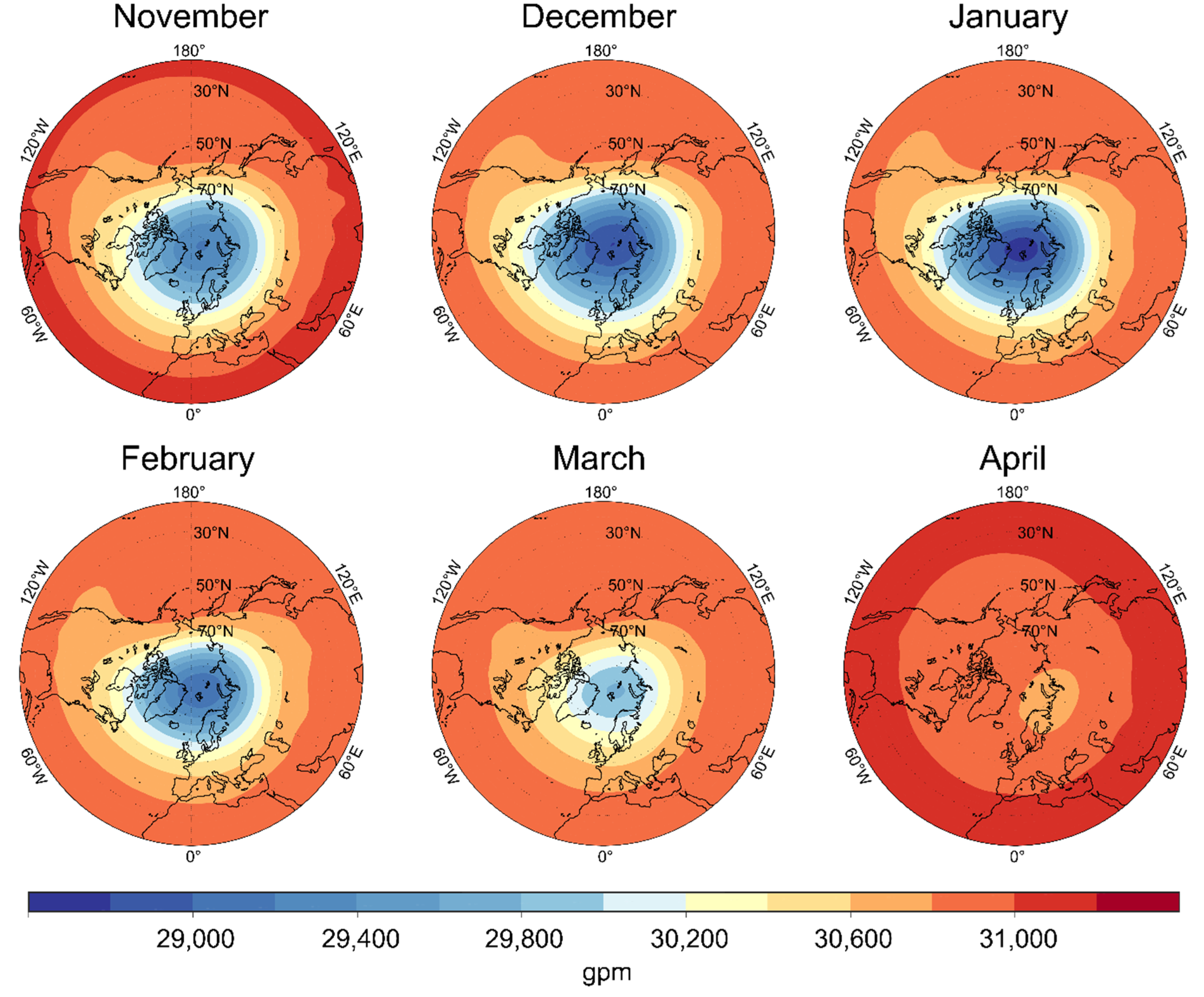
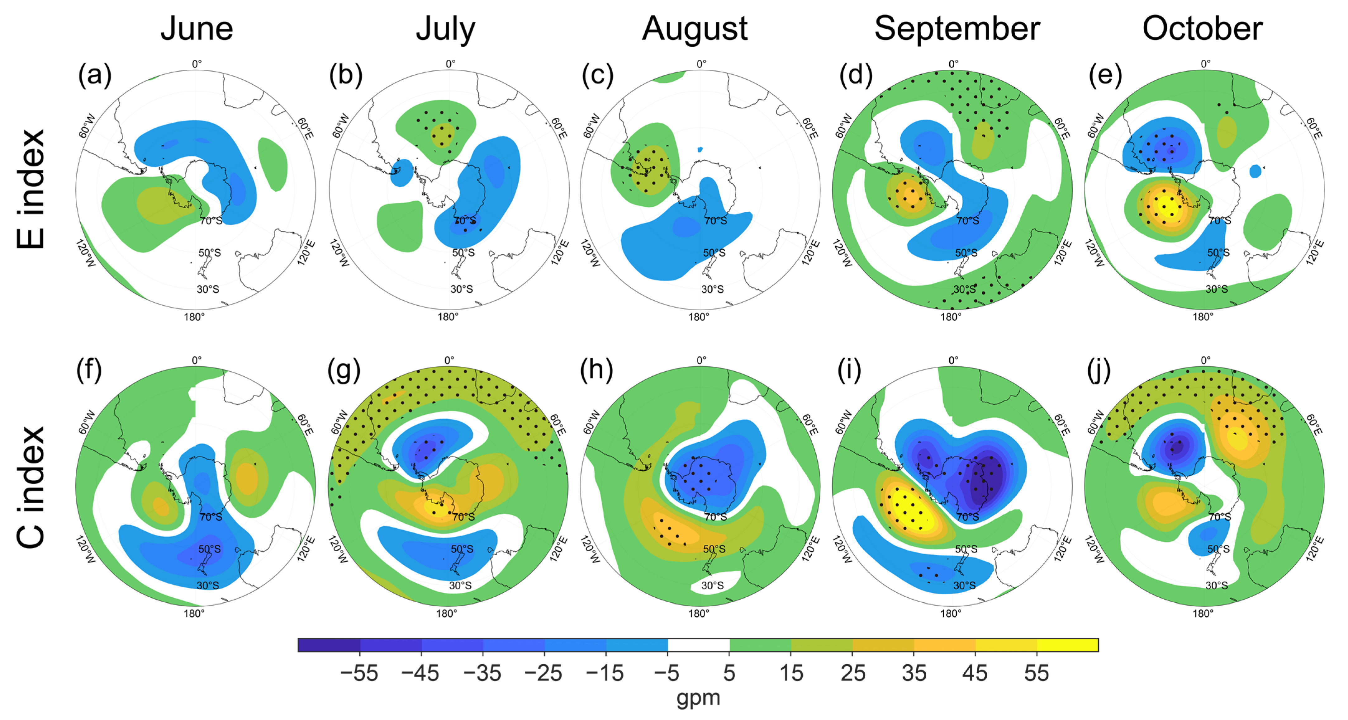
From Figure 1, we conclude that, during the cold period, low pressure encapsulates the polar region and is surrounded by a higher-pressure belt over the mid-latitudes and subtropics. The average geopotential height over the North Pole decreases from November to January and increases from February to March. Thus, the negative (positive) values of the regression coefficients in the near-polar regions can be interpreted as an increase (weakening) in the cyclonic polar vortex during the El Niño period (positive values of the E and C indices).
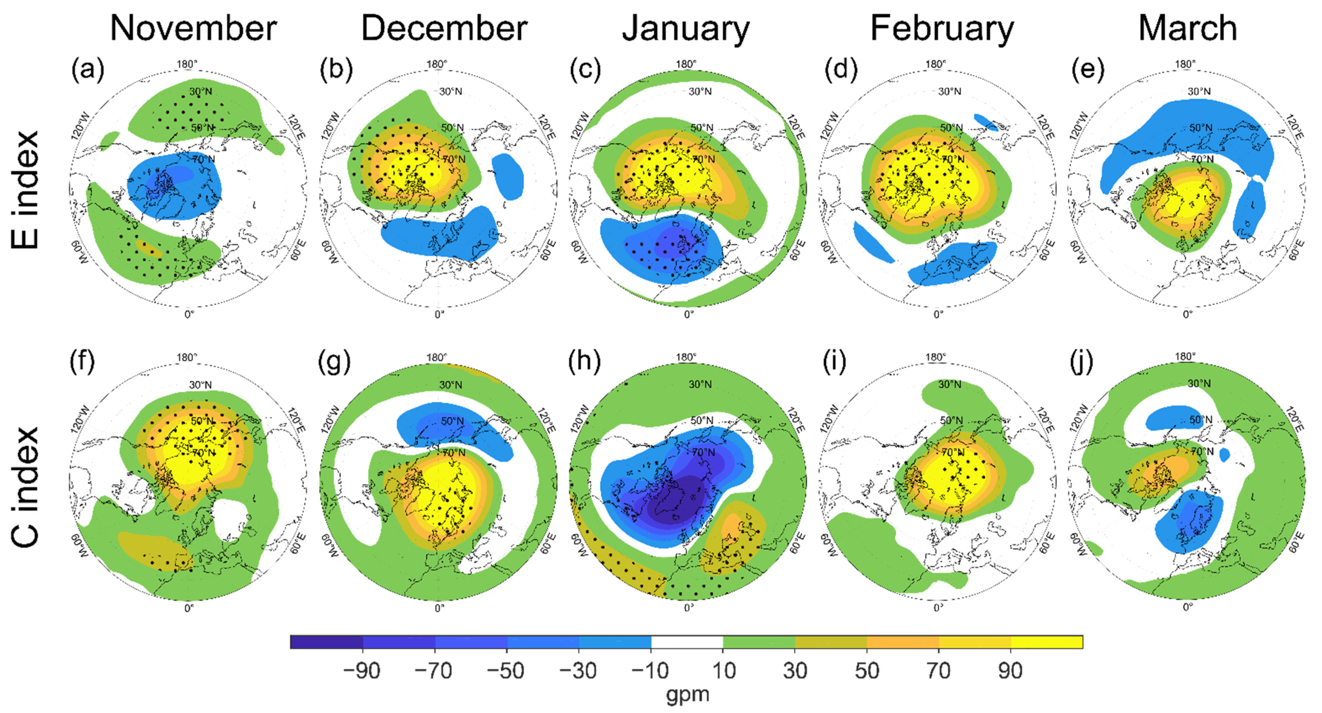
Regression analysis revealed that an increase in the equatorial Pacific SST associated with EP El Niños is related to an increase in the geopotential height over Canada and the Arctic Ocean in the middle stratosphere (10 hPa) starting in December (Figure 2b). During the next two months, the area of positive regression coefficients expands and shifts to the north, capturing the entire circumpolar region by February (Figure 2c,d). Simultaneously, the area of negative regression coefficients forms over the North Atlantic and Europe with a maximum over Iceland. In general, this distribution of geopotential height anomalies coincides with the weakening in the stratospheric polar vortex.
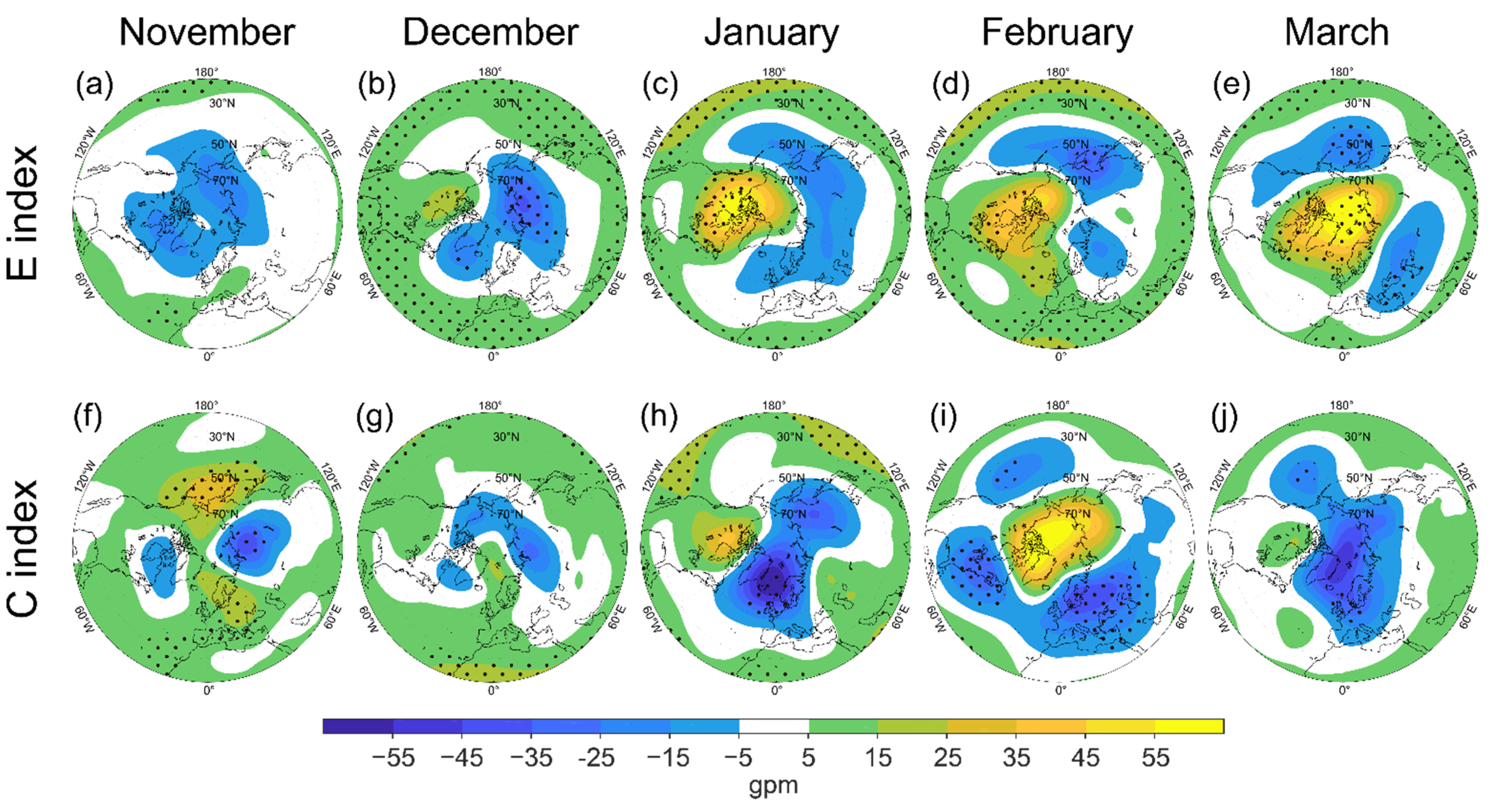
In the lower stratosphere (70 hPa), the growth in the geopotential height over the high latitudes associated with the growth in the E index begins one month later (in January). At the beginning of the cold period (November and December), the location of high and low pressure areas is similar to the mean climate conditions (i.e., low pressure over the pole and higher pressure at subtropical latitudes, Figure 3a,b). However, the intensity of the stratospheric polar vortex is higher than normal, as evidenced by negative regression coefficients localized in the circumpolar regions. In contrast to the middle stratosphere, the region of positive regression coefficients in January does not expand toward Eurasia but is enclosed over North America and the Arctic Ocean, while negative regression coefficients are observed over Eurasia, the Eastern Atlantic, and the Western Pacific (Figure 3c). In February, this pattern persists, with a minimum forming over Kamchatka and the Okhotsk Sea (Figure 3d). This may be interpreted as a shift in the low pressure center from the pole toward the Pacific. Only in March is the maximum of the regression coefficients located over the pole, which corresponds to a significant increase in pressure in this region and, consequently, a weakening in the polar vortex (Figure 3e).
During CP El Niños, the distribution of the regression coefficients drastically differs from the one observed during EP El Niños. The area of positive regression coefficients appears earlier than during EP events (in November) over the Arctic Ocean and adjacent continents in the middle stratosphere (Figure 2f) and over the Pacific and Northern Europe in the lower stratosphere (Figure 3f). Simultaneously, negative regression coefficients are observed over Eurasia and east of Canada. It corresponds to the growth in the geopotential height over the Pacific and Northern Europe and decrease in the geopotential height over Eurasia and Canada associated with the growth in the C+ index. In the meantime, on the map of mean geopotential height for November, we see the geopotential minimum centered over the pole (Figure 1). The decrease in the geopotential height over Eurasia and Canada that occurs simultaneously with increase in the geopotential height over the Pacific and Northern Europe may result from the polar vortex splitting into two centers in the lower stratosphere, with two minimums located over the continents separated by the areas with increased geopotential height over the Pacific and Northern Europe. In December and February in the middle stratosphere (Figure 2g,i), the area of positive regression is centered almost over the pole. The positive regression of the geopotential height with the C+ index suggests weakening in the stratospheric polar vortex associated with CP El Niño conditions. In contrast, during January, the regression corresponds to the strengthening in the polar vortex in response to the CP El Niño; in both the middle and lower stratosphere, negative regression coefficients appear over the pole (Figure 2h and Figure 3h) but are not statistically significant. This may result from the weakening in the wave activity flux in January during the CP events (Figure 4b and Figure 5b). This fact is in accordance with the decreased polar stratosphere temperature (Figure 6b) and accelerated westerly zonal flow (Figure 7b) observed in January of CP El Nino years. In the lower stratosphere, the positive geopotential height anomalies in the circumpolar regions responding to the CP El Niño appear only in February (Figure 3i). During the rest of the cold period, no weakening in the polar vortex in the lower stratosphere in response to CP El Niños is observed. At moderate latitudes in the lower stratosphere, the belt of negative regression forms in February and corresponds to negative geopotential height anomalies in this area (Figure 3i). The opposite patterns of circulation anomalies associated to EP and CP El Niños emerge in the lower stratosphere in March (Figure 3e,j), with positive (negative) regressions centered over the North Pole during EP (CP) El Niño conditions. This indicates delayed spring restructuring of stratospheric circulation into summer anticyclone after CP events. Note, this feature is less pronounced in the middle stratosphere (Figure 2e,j).
Previous studies showed that the weakening in the stratospheric polar vortex during El Niño events is due to intensification in wave activity flux into the stratosphere [16,17,18]. El Niño leads to the deepening of the Aleutian low, which results in increased wave activity and stronger upward wave activity flux into the stratosphere [15].
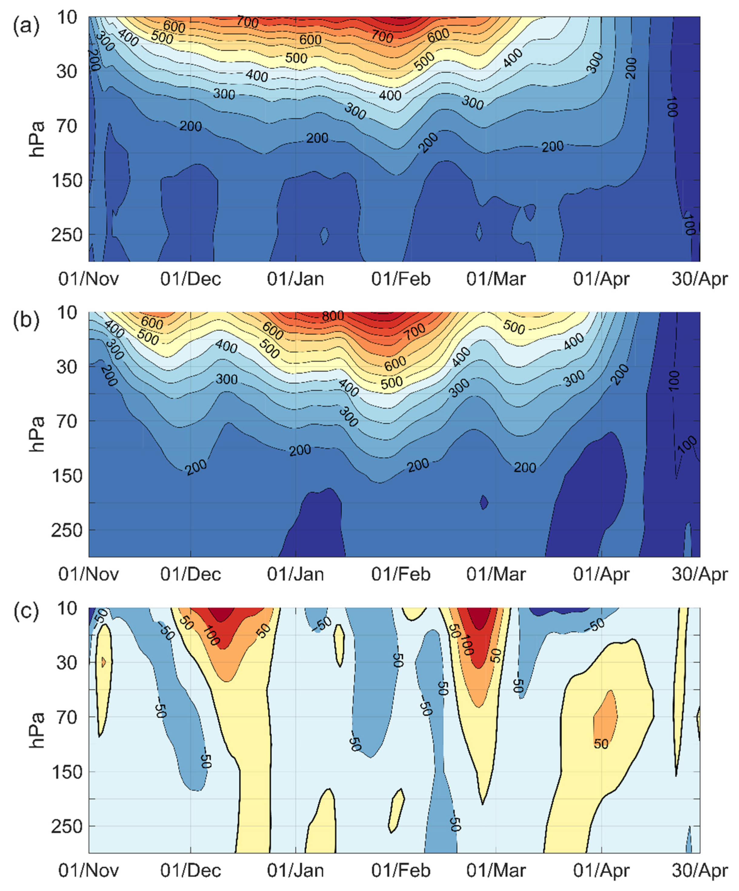
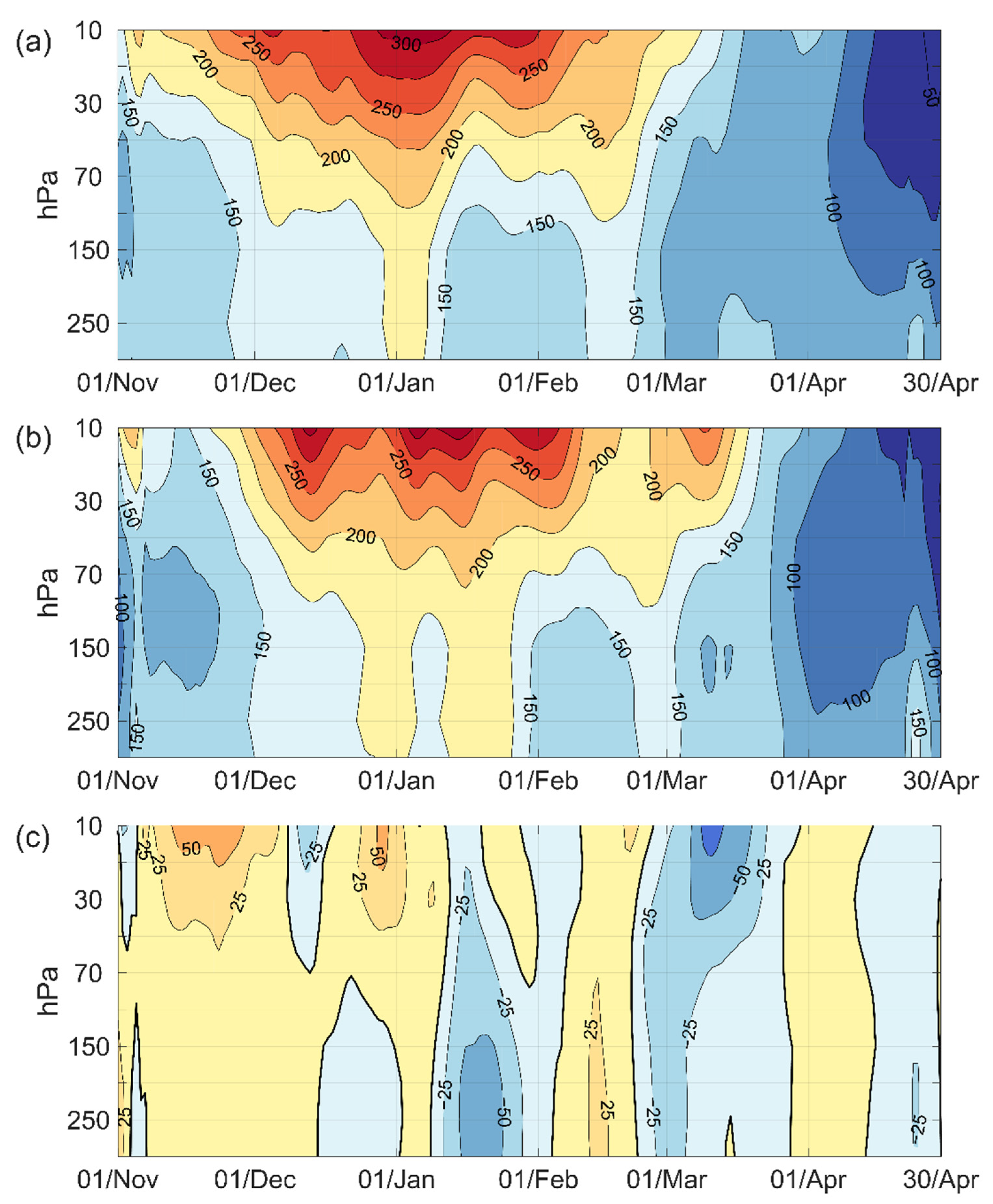
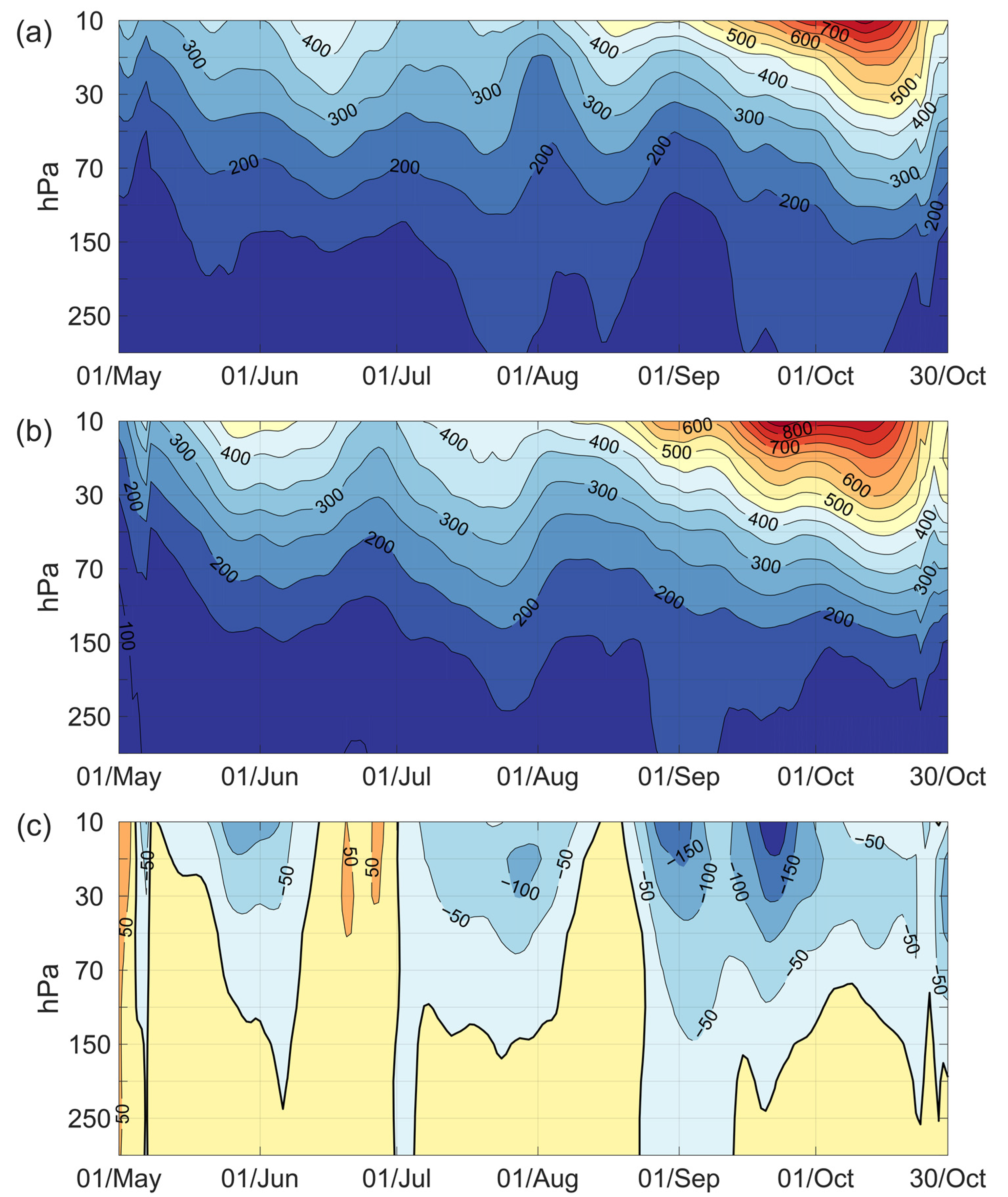
To analyze these changes in wave activity, the composites of the amplitude of planetary waves with zonal wave numbers 1 and 2 averaged over 50 to 70° N during EP and CP El Niño events as well as the difference between them were plotted for the boreal cold season (Figure 4 and Figure 5). The cold season is identified in accordance with the typical period of polar stratospheric vortex occurring from November to April. Figure 4 shows that a higher amplitude in the wave with zonal wave number 1 is associated with EP El Niños compared to the CP events in December and late February to early March. Near 10 hPa, the difference between the composites reaches 120 gpm. In the rest of the cold season, the difference is negligible.
The amplitude of the wave with zonal wave number 2 is greater during EP events in November to December and lower in March, with less difference between the CP and EP composites as compared to the wave with zonal wave number 1 (Figure 5).
These results are consistent with Ref. [53] and demonstrate the larger amplitude of the wave with zonal wave number 1 during EP events, leading to enhanced weakening in the stratospheric vortex compared to CP El Niños.
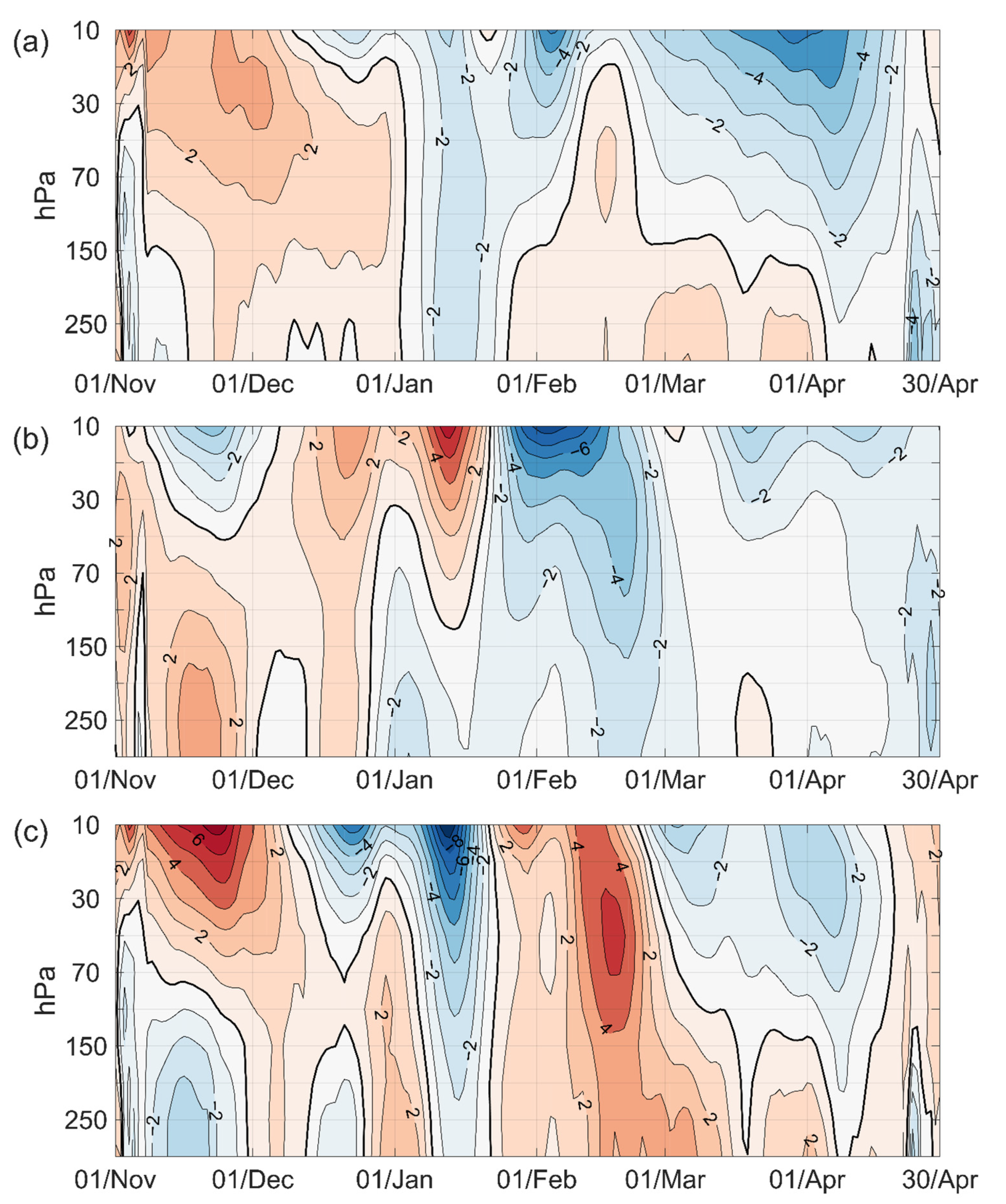
The intensification in the wave activity flux during El Niño contributes to larger heat flux from the troposphere into the stratosphere that, in turn, increases the polar stratosphere temperature. The warmer stratosphere leads to a slowdown of the westerly current and the weakening in the polar vortex. To show the imprint of El Niño on the stratosphere meteorological parameters, the composites of the Arctic stratosphere daily temperature anomalies averaged between 70 and 90° N and zonal mean wind speed anomalies at 60° N during EP and CP El Niño events as well as the difference between them were plotted (Figure 6 and Figure 7). The chosen latitudinal belt corresponds to the area of maximum intensity of the analyzed meteorological parameters.
Composites for Arctic stratosphere temperature show that the temperature in the middle and lower Arctic stratosphere is higher in the years of EP compared to CP El Niño (Figure 6a,b). The maximum difference, up to 7 to 8 °C, is observed near 10 hPa from mid-December to mid-January (Figure 6c) when the strong positive anomalies are observed during EP El Niño and negative anomalies during CP events. However, in February, the situation is the opposite: higher temperatures are observed during the years of the CP El Niño (Figure 6c), with the positive temperature anomalies during CP El Niño being twice as high as during the EP event (Figure 6a,b).
The composite analysis for zonal wind coincides with polar stratospheric temperatures. The negative anomalies of westerly winds are observed during the whole winter of EP El Niño years and since mid-January of CP El Niño years, which corresponds to the weakening in the zonal flow associated with ENSO. The anomalies have a larger magnitude for EP events (Figure 7a), indicating the zonal wind is weaker during the EP El Niño (with the maximum difference in December and January by 6 to 8 m/s) compared to CP El Niños (Figure 7a–c), confirming the lower intensity in the stratospheric polar vortex associated with EP El Niños.
3.2. Stratospheric Circulation Response to Two Types of El Niño in the Southern Hemisphere
An analysis of the stratospheric circulation anomalies associated with the two types of El Niño analogous to the NH was carried out for the SH.
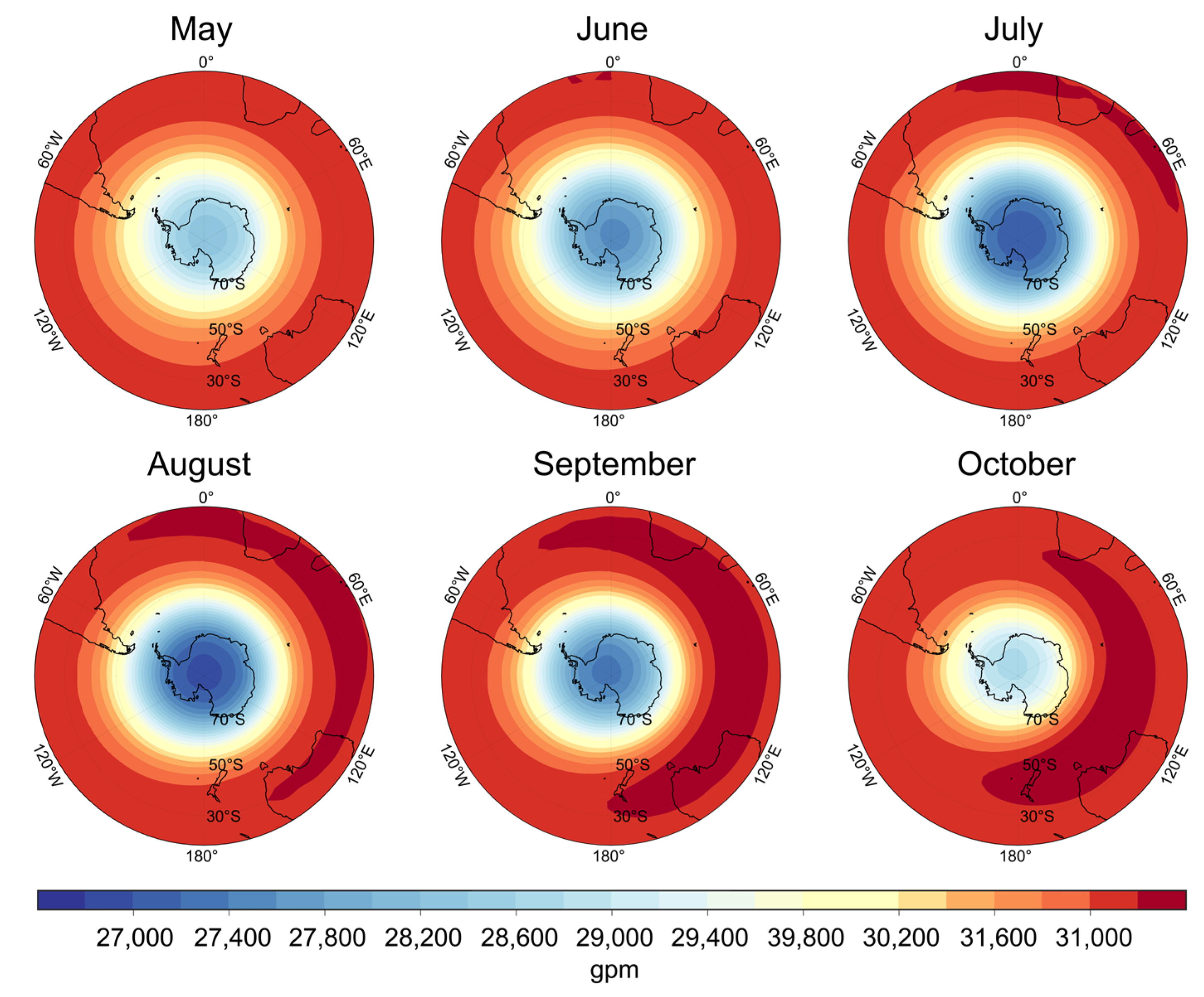
Firstly, note the difference in the mean climate conditions in the northern and southern polar stratospheres. The stratospheric polar vortex formed during the cold period in the SH is much more intense and isolated than its counterpart in the NH. The air temperatures in the Antarctic stratosphere are lower than those in the Arctic, and the zonal wind speed is about twice as high as in the Arctic. The stratospheric polar vortex in the SH, unlike its counterpart, reaches its maximum intensity not in the middle of boreal summer but in August, and the change in the zonal current direction from westerly to easterly occurs in November (Figure 1 and Figure 8).
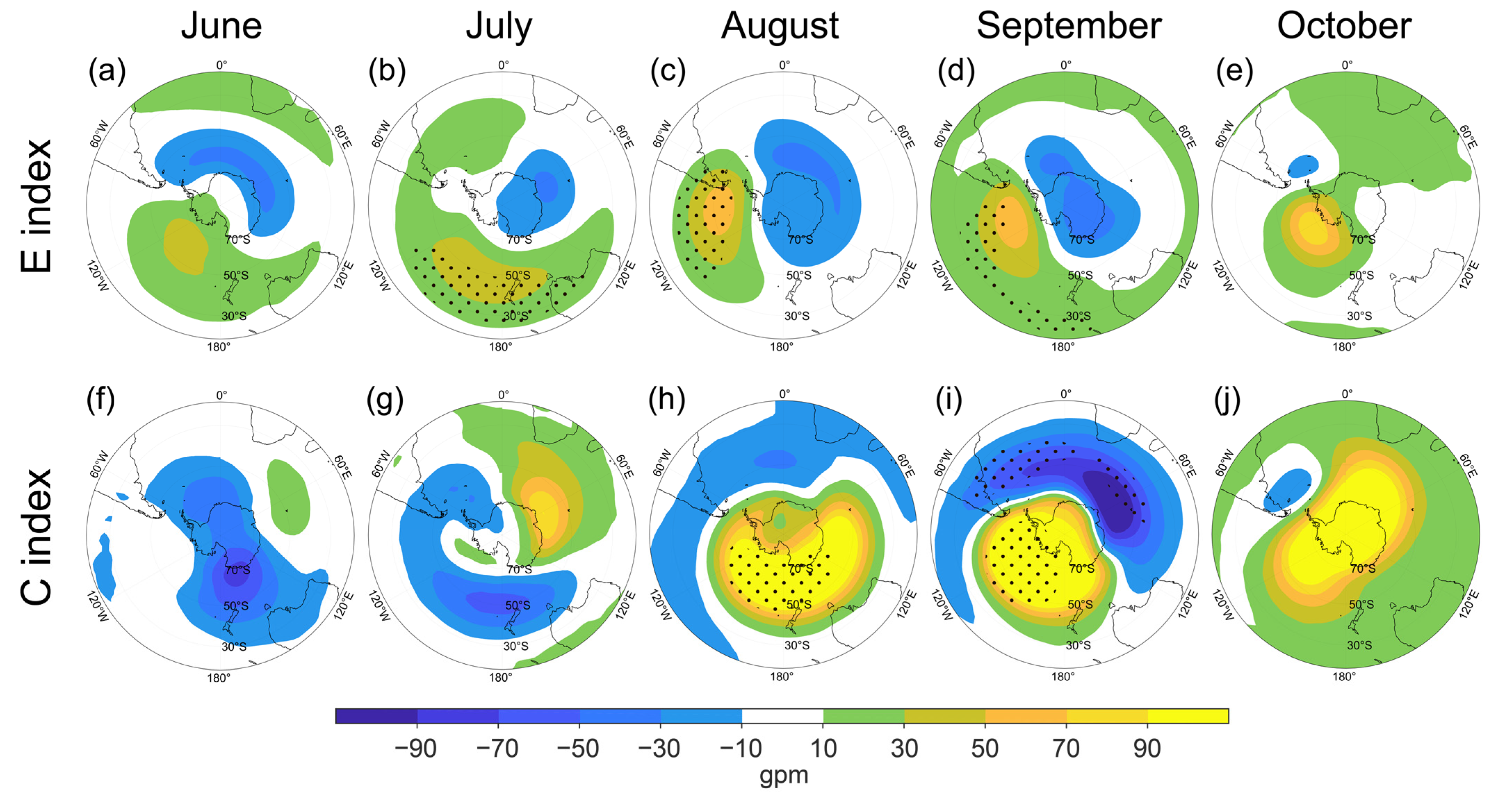
Previous investigations showed that, in the SH, the maximum circulation anomalies and increased wave activity associated with ENSO occur in September and October preceding the peak of El Niño [27,29,30]. This is due to two reasons: (1) the Antarctic polar vortex reaches its highest intensity in August; (2) despite the fact that El Niño commonly peaks in December–January, the maximum growth of SST anomalies in the equatorial Pacific during El Niño occurs during austral spring [26]. For these reasons, we performed the regression and composite analysis for the winter–spring period preceding the peak of the Eastern and Central Pacific El Niño events.
The linear relationship between El Niño and the circulation of the middle and lower stratosphere was analyzed based on synchronous regressions of geopotential height anomalies at 70 and 10 hPa onto El Niño indices for the cold season of the SH (June–October).
The middle stratospheric circulation changes that are related to the two types of El Niño are dramatically different (Figure 9). During EP El Niño development (June–September), the weak negative regression coefficients appear in the near-polar regions but are not statistically significant (Figure 9a–d). This suggests that there is no weakening in the stratospheric polar vortex in response to the EP El Niño in the SH. The area of positive regression coefficients corresponding to the geopotential growth appears in June over the Pacific, persists in July, and shifts toward South America in August–September (Figure 9a–d). Only during October (Figure 9e) does it move toward the South Pole; however, it is most likely associated with the spring restructuring in the stratosphere to the summer form of circulation than to polar vortex weakening in response to the EP El Niño.
In contrast to the EP El Niño, the weakening in the polar vortex appears to respond to CP events in August–September (Figure 9h,i). However, the maximum is not centered over the pole but rather shifted toward the South Pacific and Western Antarctica. In October, the area of positive regression coefficients during CP El Niños captures the entire polar region; however, the values of the regression coefficients are not statistically significant. This is likely due to the fact that remote El Niño forcing in October does not play a significant role in the stratospheric circulation. The radiation factors dominate, affecting the restructuring of the stratospheric circulation from winter to summer.
The response of the lower stratosphere (70 hPa) polar circulation to EP El Niño is similar to the middle stratosphere, where no weakening in the stratospheric polar vortex is observed (Figure 10a–e). Meanwhile, the anomalies associated with CP El Niño are almost the opposite to those observed in the middle stratosphere. In August and September, intensification in the polar vortex occurs (negative regression coefficients between C+ index and geopotential height anomalies) and positive regressions are located over the South Pacific.
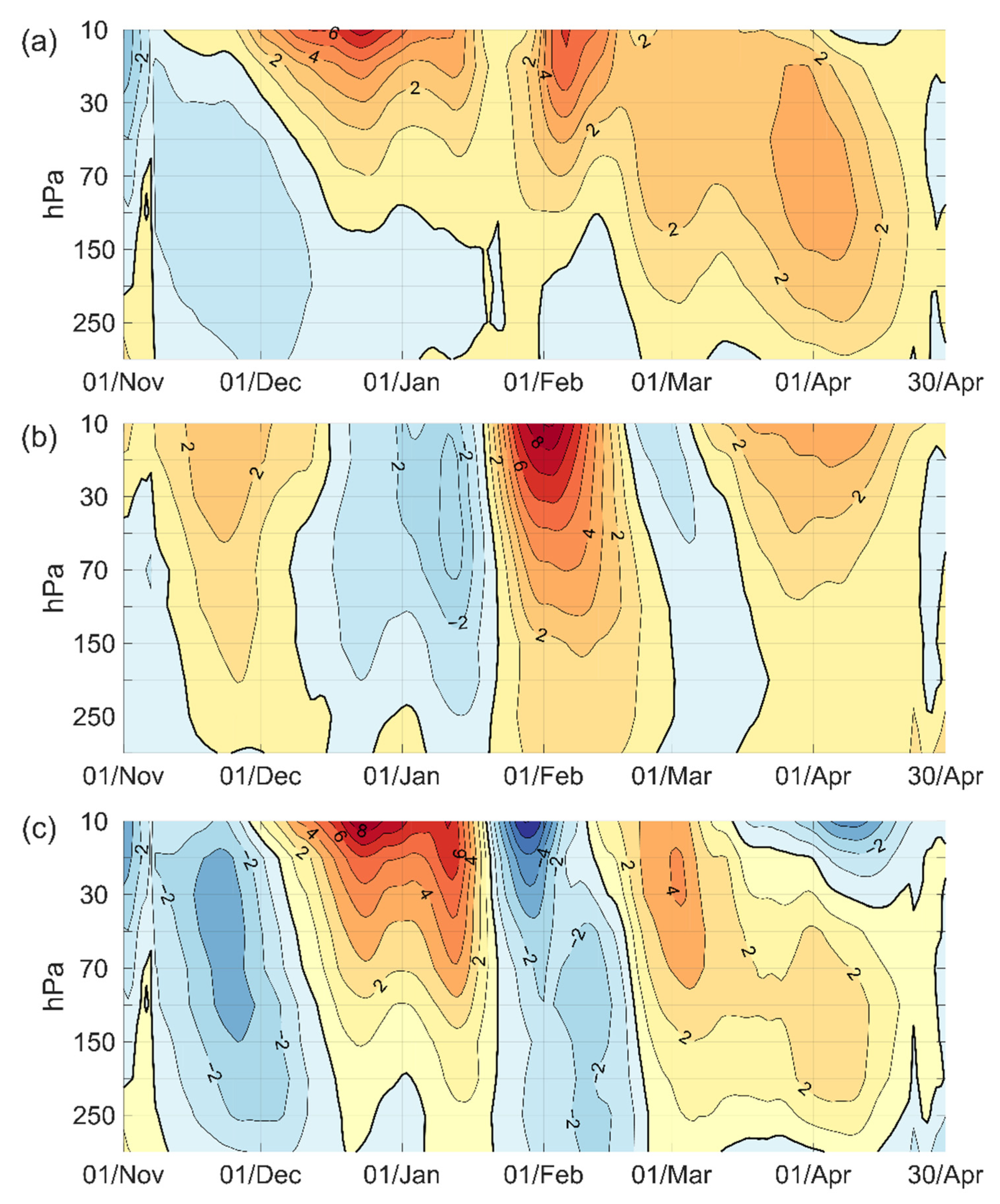
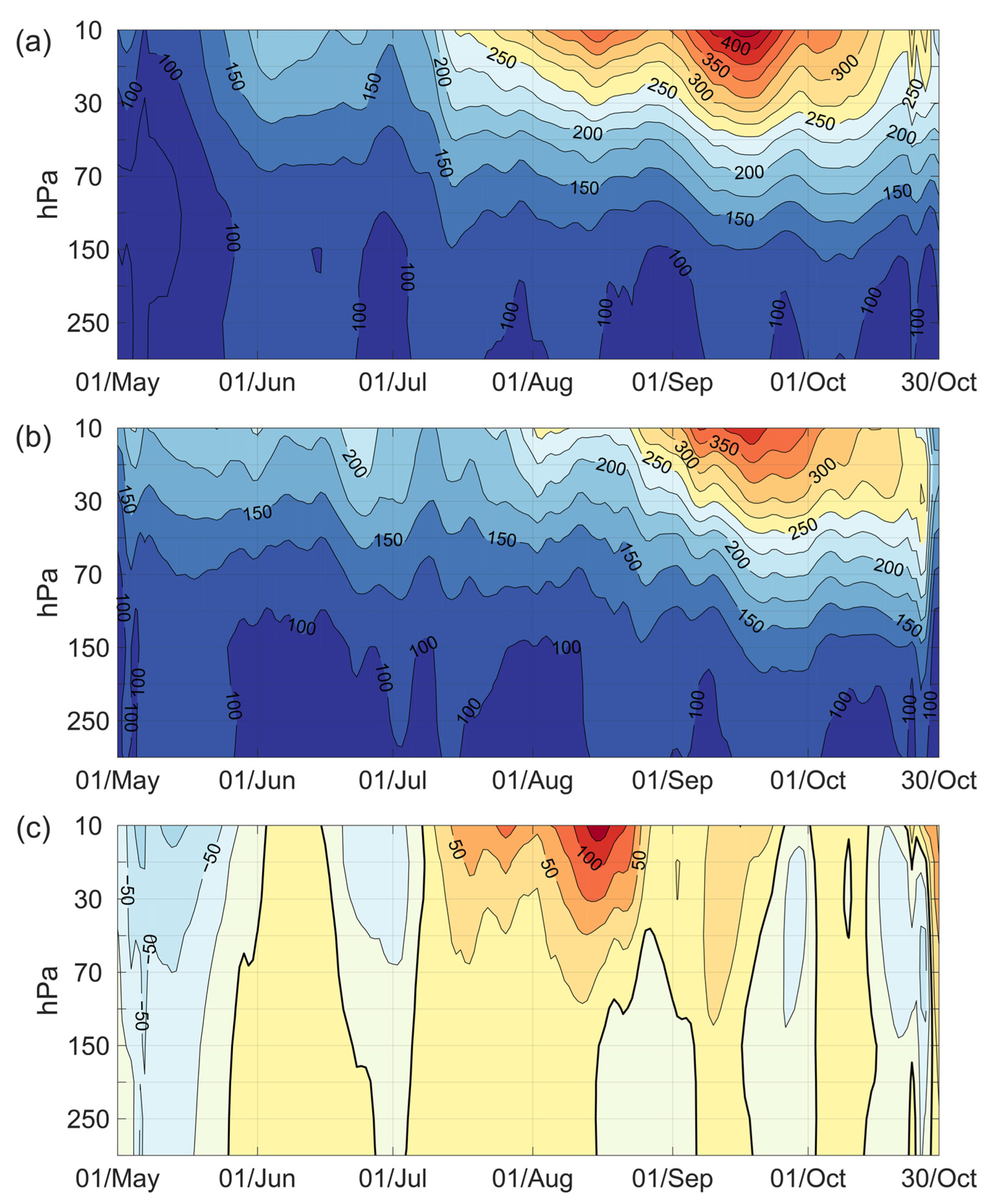
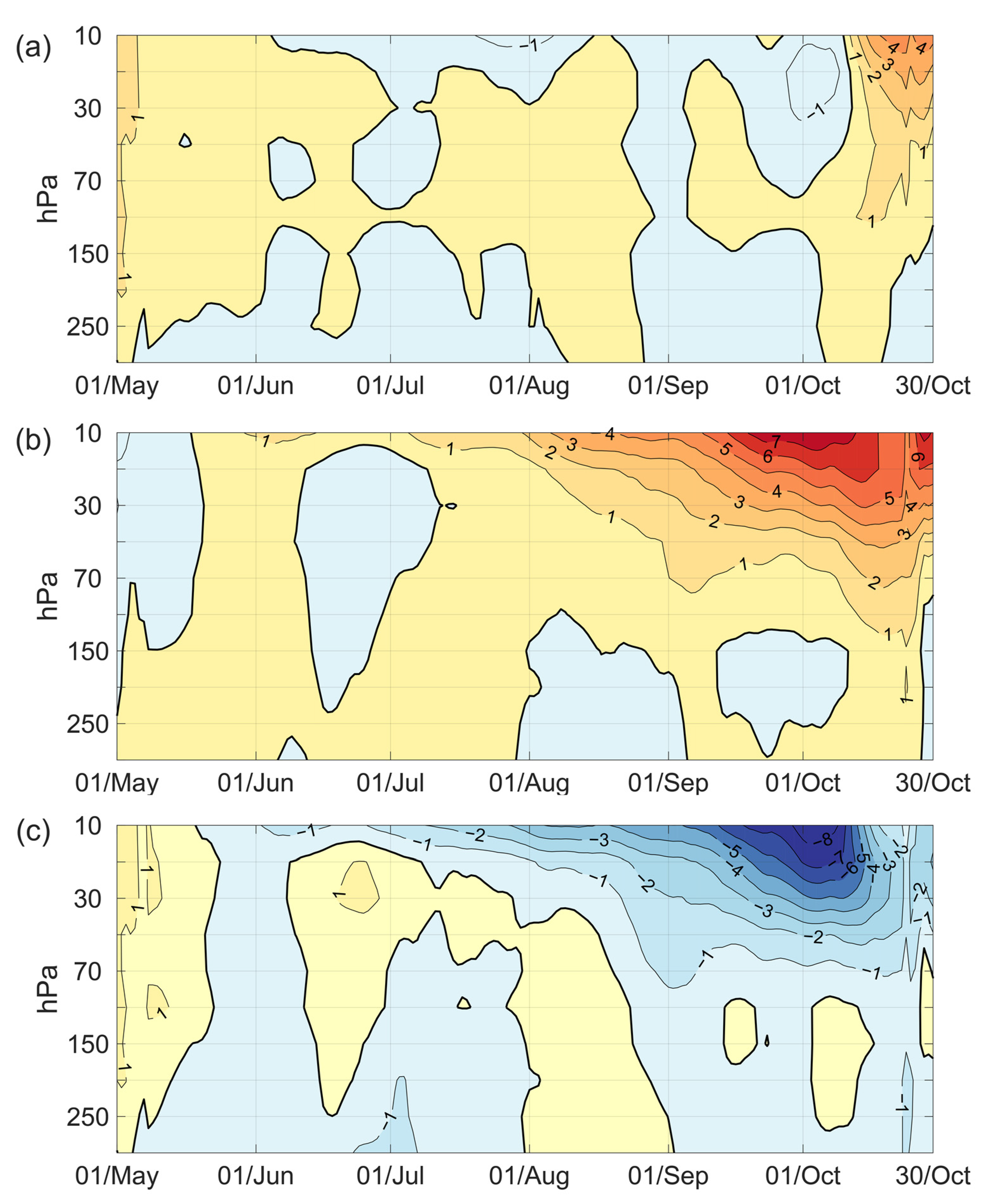
An analysis of the amplitudes of planetary waves with a zonal wave number 1 showed that their intensity is higher in the seasons of CP El Niño (Figure 11). The maximum differences are observed in early August (100 gpm) and September (more than 200 gpm). This coincides with the more important weakening in the polar vortex in the middle stratosphere occurring under CP El Niño conditions in the SH (Figure 9h,i).
In contrast, the higher amplitude of the wave with zonal wave number 2 is associated with EP El Niños (Figure 12a), with the maximum difference observed in July and August exceeding 100 gpm (Figure 12c).
The main differences in the Antarctic stratospheric temperatures between the two types of El Niño are observed from August to October (Figure 13). The temperature in the middle stratosphere is higher during CP El Niños as compared to EP El Niños, with the maximum difference occurring in early October (more than 8 °C). This is in accordance with planetary wave activity that is greater during CP events.
Consistent with the difference in polar vortex weakening, the zonal mean wind speed at 60° S in the middle stratosphere is lower during CP El Niños than during EP El Niños over the entire cold season of the SH, with the negative anomalies observed in CP years and small positive anomalies during EP (Figure 14a,b). The difference between the composites amounts to 4–6 m/s, with the maximum observed in late September–early October (Figure 14c).
4. Discussion and Conclusions
Based on reanalysis data, we investigated the remote response to ENSO in the mid- to high latitude stratosphere, focusing on the inter-event variability likely resulting from the existence of two ENSO types—the Eastern and Central Pacific El Niños. Moreover, considering previous results that highlight the clear interhemispheric difference of ENSO teleconnection in the troposphere [2], we analyzed the ENSO response in the stratosphere of mid- to high latitudes for the Northern and Southern Hemispheres. Our study complements previous research (e.g., Refs. [16,17,18,22,23,24,25,31,32,33,34,36]) that showed a weakening in the stratospheric polar vortex associated with El Niños and inhomogeneity in the NH polar vortex response to El Niños during the cold season [59]. We emphasize that both of these features of polar stratospheric response strongly depend on the ENSO types and differ between the hemispheres as well as the lower to middle stratosphere.
We show that weakening in the stratospheric polar vortex in the Arctic is observed in the middle stratosphere throughout the winter months in response to EP El Niños, while the circulation patterns associated with CP El Niño show the polar vortex weakening in November, December, and February and strengthening in January. Thus, the response of the middle stratospheric circulation is similar for the two types of El Niño in December and February and is the opposite in November and January. The difference in November is due to polar vortex weakening beginning later during EP events. In January, it is due to weakened wave activity flux and the associated decrease in stratosphere temperature and strengthening in the westerly current associated with CP El Niños. In the lower stratosphere, the weakening in the polar vortex is less evident than in the middle stratosphere and starts in January of EP El Niño years, while, during CP events, it manifests only in February. Therefore, the middle and lower stratospheric circulation response is similar for EP events in the second part of the cold season and is almost the opposite for CP events except for January.
In the SH, the relationship between El Niño and the stratospheric polar vortex was investigated for the austral late winter and early spring months before the peak of El Niño. During this period of the year, the growth rate of SST anomalies in the equatorial Pacific Ocean is maximum and the influence of radiation processes in the restructuring of the stratospheric circulation within the seasonal cycle is still weak. We found that the influence of El Niño on the stratospheric polar vortex occurs only in the case of the CP El Niño in August and September before the peak of El Niño. Another important difference in the SH stratosphere response to EP and CP El Niños is the opposite circulation patterns in the middle and lower stratosphere during CP events and similar structure during EP events. The main stratosphere interhemispheric asymmetry manifests in the response to EP El Niños that is not significant in the SH, while the CP events are associated with enhanced weakening in the polar vortex in both hemispheres.
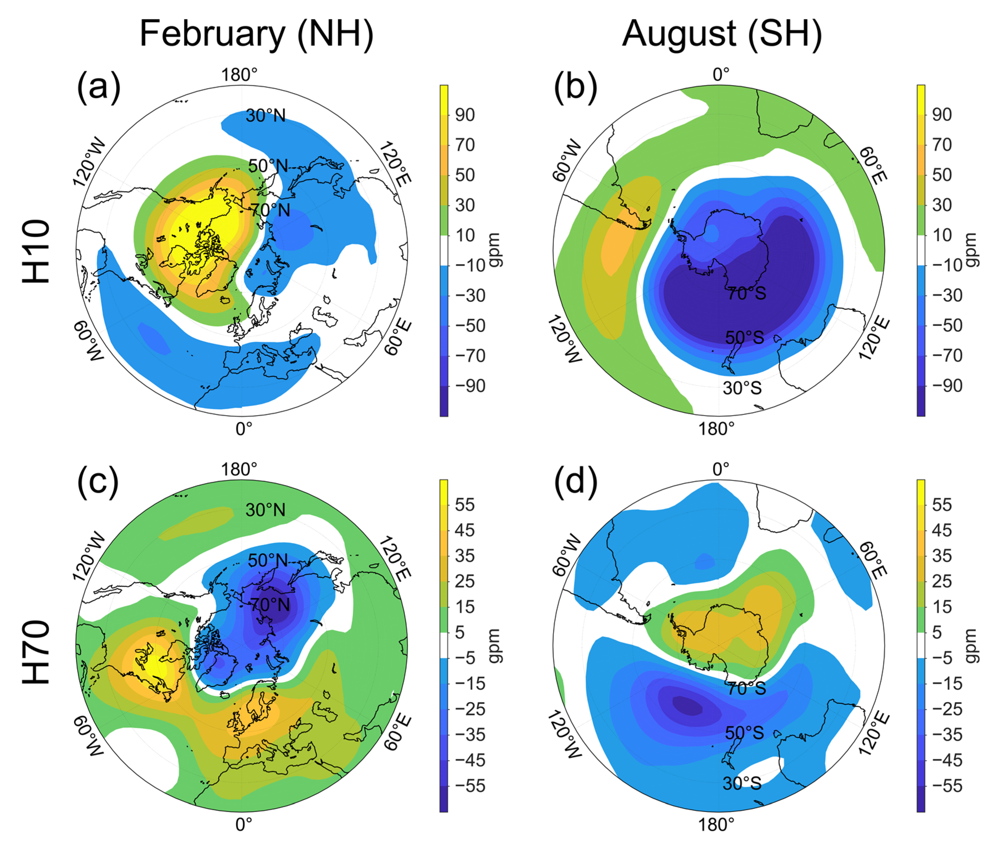
To illustrate the diversity of the polar stratospheric circulation response to two types of El Niño, we present maps of the differences between the geopotential height regression onto the E and C+ indices in the lower and middle stratosphere of the Northern and Southern Hemispheres (Figure 15). As the response changes during the cold season, we chose the months when the maximum polar vortex weakening was observed: February in the NH and August in the SH. Noticeably, the difference between the events is the opposite for the middle (Figure 15a,b) and lower (Figure 15c,d) stratosphere as well as for the NH (Figure 15a,c) and SH (Figure 15b,d). The weakening in the polar vortex in the middle stratosphere is more pronounced during the EP El Niño in the NH and CP El Niño in the SH. The opposite structure is observed in the lower stratosphere, where the strengthening in the SH vortex in August of CP El Niño years is observed.
The results of this study, combined with previous investigation [2], allow to highlight the dramatic difference between the ENSO/polar circulation relationships in the troposphere and the stratosphere. The boreal winter stratospheric and tropospheric responses to CP events in the NH and both types of ENSO in the SH may be approximated by an annular mode centered over the polar and subpolar regions, while the wave pattern emanating from the tropics poleward in December to February is associated with EP El Niños and is confined within the troposphere. The wavetrain in the SH manifests only in the troposphere during austral winter [31,32]. Therefore, the stratospheric response is likely due to vertically rather than meridionally propagating waves. The question as to why the wave response is not observed in the NH troposphere after CP events and after both ENSO types in the SH during austral summer remains open.
Another open question concerns the possible modification of the ENSO/stratosphere teleconnection in the future climate. This issue was addressed in several studies (e.g., Refs. [1,60]) that suggest the weakening in the stratospheric response to ENSO in the future climate. Meanwhile, in Ref. [2], it was showed that, in the troposphere in the warmer climate, the circulation response in the high latitudes to both types of events in the opposite is amplified in both hemispheres. However, it is difficult to analyze the projected changes in the ENSO/stratosphere teleconnection in the future climate using the CMIP5 model ensemble, taking into account the strong intermodel discrepancy in the simulation of the stratosphere circulation response to El Niño as well as significant differences between the teleconnection patterns for CP El Niño simulated by CMIP5 models in a “historical” run (experiment that covers the period from 1916 to 2005 and consists of simulations where the observed changes in air composition (including CO2) were due to both anthropogenic and volcanic impacts [61]) and NCEP/NCAR reanalysis (Figures S1 and S2, Supplementary Materials [2,61,62,63]). The further investigations using the improved models of the CMIP6 project may address this issue.
Supplementary Materials
The following supporting information can be downloaded at: https://www.mdpi.com/article/10.3390/atmos13050682/s1, Figure S1: Regression of geopotential height anomalies at 10 hPa onto E index (first two columns) and C+ index (second two columns) from November to March in NCEP-NCAR reanalysis (first and third columns) and in ensemble mean of the selected CMIP5 models (second and fourth columns). Dotted areas represent statistically significant values at a 90% confidence level. Contour interval is 20 gpm. The outermost latitude is 20° N; Figure S2: Regression of geopotential height anomalies at 70 hPa onto E index (first two columns) and C+ index (second two columns) from November to March in NCEP-NCAR reanalysis (first and third columns) and in ensemble mean of the selected CMIP5 models (second and fourth columns). Dotted areas represent statistically significant values at a 90% confidence level. Contour interval is 20 gpm. The outermost latitude is 20° N.
Author Contributions
Conceptualization, D.G.; methodology, D.G. and M.K.; software, M.K.; validation, M.K. and D.G.; formal analysis, M.K. and D.G.; investigation, M.K. and D.G.; writing—original draft preparation, M.K. and D.G.; writing—review and editing, D.G.; visualization, M.K.; supervision, D.G. All authors have read and agreed to the published version of the manuscript.
Funding
The research was funded by Lomonosov Moscow State University (AAAA-A16-116032810086-4) and MSU Interdisciplinary Scientific and Educational School Development Program “The Future of the Planet and the Development of the Environment”.
Data Availability Statement
The datasets analyzed and generated during our study are available on request to corresponding authors.
Acknowledgments
The study is carried out in frame of scientific program of the Faculty of Geography of Moscow State University no AAAA-A16-116032810086-4 and MSU Interdisciplinary Scientific and Educational School Development Program “The Future of the Planet and the Development of the Environment”. We are grateful to Eugeniy Volodin for discussions on the calculation of wave amplitude.
Conflicts of Interest
The authors declare no conflict of interest.
References
- Domeisen, D.I.; Garfinkel, C.I.; Butler, A.H. The teleconnection of El Niño Southern Oscillation to the stratosphere. Rev. Geophys. 2019, 57, 5–47. [Google Scholar] [CrossRef] [Green Version]
- Gushchina, D.; Kolennikova, M.; Dewitte, B.; Yeh, S.-W. On the relationship between ENSO diversity and the ENSO atmospheric teleconnection to high-latitudes. Int. J. Climatol. 2021, 42, 1303–1325. [Google Scholar] [CrossRef]
- Thompson, D.; Wallace, J. Observed linkages between Eurasian surface air temperature, the North Atlantic Oscillation, Arctic sea level pressure and the stratospheric polar vortex. Geophys. Res. Lett. 1998, 25, 1297–1300. [Google Scholar] [CrossRef] [Green Version]
- Baldwin, M.P.; Dunkerton, T.J. Propagation of the Arctic Oscillation from the stratosphere to the troposphere. J. Geophysical Research 1999, 104, 430–937. [Google Scholar] [CrossRef]
- Baldwin, M.P.; Dunkerton, T.J. Stratospheric harbingers of anomalous weather regimes. Science 2001, 294, 581–584. [Google Scholar] [CrossRef] [PubMed]
- Kuroda, K. Relationship between the Polar-Night Jet Oscillation and the Annular Mode. Geophys. Res. Lett. 2002, 29, 1240. [Google Scholar] [CrossRef] [Green Version]
- Black, R.; McDaniel, B.; Robinson, W.A. Stratosphere-troposphere coupling during spring onset. J. Clim. 2006, 19, 4891–4901. [Google Scholar] [CrossRef]
- Li, Y.; Lau, N.-C. Influences of ENSO on stratospheric variability, and the descent of stratospheric perturbations into the lower troposphere. J. Clim. 2013, 26, 4725–4748. [Google Scholar] [CrossRef] [Green Version]
- Cheung, H.N.; Zhou, W.; Leung, M.Y.T.; Shun, C.M.; Lee, S.M.; Tong, H.W. A strong phase reversal of the Arctic Oscillation in midwinter 2015/2016: Role of the stratospheric polar vortex and tropospheric blocking. J. Geophys. Res. Atmos. 2016, 121, 13443–13457. [Google Scholar] [CrossRef]
- Manney, G.L.; Santee, M.L.; Rex, M.; Livesey, N.J.; Pitts, M.C.; Veefkind, P.; Nash, E.R.; Wohltmann, I.; Lehmann, R.; Froidevaux, L.; et al. Unprecedented Arctic ozone loss in 2011. Nature 2011, 478, 469. [Google Scholar] [CrossRef]
- Rao, J.; Garfinkel, C.I. Arctic Ozone Loss in March 2020 and Its Seasonal Prediction in CFSv2: A Comparative Study with the 1997 and 2011 Cases. J. Geophys. Res. Atmos. 2020, 125, e2020JD033524. [Google Scholar] [CrossRef]
- Matsuno, T. A dynamical model of stratospheric sudden warming. J. Atmos. Sci. 1971, 28, 1479–1494. [Google Scholar] [CrossRef]
- Charney, J.; Drazin, P. Propagation of planetary-scale disturbances from the lower into the upper atmosphere. J. Geophys. Res. 1961, 66, 83–109. [Google Scholar] [CrossRef]
- Gavrilov, N.M.; Koval, A.V.; Pogoreltsev, A.I.; Savenkova, E.N. Simulating planetary wave propagation to the upper atmosphere during stratospheric warming events at different mountain wave scenarios. Adv. Space Res. 2018, 61, 1819–1836. [Google Scholar] [CrossRef]
- Van Loon, H.; Labitzke, K. The Southern Oscillation.Part V: The anomalies in the lower stratosphere of the Northern Hemisphere in winter and a comparison with the quasi-biennial oscillation. Mon. Weather Rev. 1987, 115, 357–369. [Google Scholar] [CrossRef] [Green Version]
- Baldwin, M.P.; O’Sullivan, D. Stratospheric effects of ENSO related tropospheric circulation anomalies. J. Clim. 1995, 8, 649–667. [Google Scholar] [CrossRef] [Green Version]
- Manzini, E.; Giorgetta, M.A.; Esch, M.; Kornblueh, L.; Roeckner, E. The influence of sea surface temperatures on the northern winter stratosphere: Ensemble simulations with the MAECHAM5 model. J. Clim. 2006, 19, 3863–3881. [Google Scholar] [CrossRef]
- Garfinkel, C.I.; Hartmann, D.L. Different ENSO teleconnections and their effects on the stratospheric polar vortex. J. Geophys. Res. 2008, 113, D18114. [Google Scholar] [CrossRef] [Green Version]
- Hoskins, B.J.; Karoly, D.J. The Steady Linear Response of a Spherical Atmosphere to Thermal and Orographic Forcing. J. Atmos. Sci. 1981, 38, 1179–1196. [Google Scholar] [CrossRef] [Green Version]
- Trenberth, K.E.; Branstator, G.W.; Karoly, D.; Kumar, A.; Lau, N.-C.; Ropelewski, C. Progress during TOGA in unferstanding and modeling global teleconnections associated with tropical sea surface temperatures. J. Geophys. Res. 1998, 103, 14291–14324. [Google Scholar] [CrossRef]
- Calvo, N.; Iza, M.; Hurwitz, M.M.; Manzini, E.; Peña-Ortiz, C.; Butler, A.H.; Cagnazzo, C.; Ineson, S.; Garfinkel, C.I. Northern Hemisphere stratospheric pathway of different El Niño flavors in CMIP5 models. J. Clim. 2017, 30, 4351–4371. [Google Scholar] [CrossRef] [Green Version]
- Garfinkel, C.I.; Hartmann, D.L. Effects of the El Niño Southern Oscillation and Quasi-Biennial Oscillation on polar temperatures in the stratosphere. J. Geophys. Res. 2007, 112, D19112. [Google Scholar] [CrossRef] [Green Version]
- Free, M.; Seidel, D.J. Observed El Niño—Southern Oscillation temperature signal in the stratosphere. J. Geophys. Res. 2009, 114, D23108. [Google Scholar] [CrossRef]
- Iza, M.; Calvo, N.; Manzini, E. The stratospheric pathway of La Niña. J. Clim. 2016, 29, 8899–8914. [Google Scholar] [CrossRef]
- Plumb, R.A. On the seasonal cycle of stratospheric planetary waves. Pure Appl. Geophys. 1989, 130, 233–242. [Google Scholar] [CrossRef]
- Li, T. Phase transition of the El Niño-Southern oscillation: A stationary SST mode. J. Atmos. Sci. 1997, 54, 2872–2887. [Google Scholar] [CrossRef] [Green Version]
- Hurwitz, M.M.; Newman, P.A.; Oman, L.D.; Molod, A.M. Response of the Antarctic stratosphere to two types of El Niño events. J. Atmos. Sci. 2011, 68, 812–822. [Google Scholar] [CrossRef] [Green Version]
- Hurwitz, M.M.; Song, I.S.; Oman, L.D.; Newman, P.A.; Molod, A.M.; Frith, S.M.; Nielsen, J.E. Response of the Antarctic stratosphere to warm pool El Niño events in the GEOS CCM. Atmos. Chem. Phys. 2011, 11, 9659–9669. [Google Scholar] [CrossRef] [Green Version]
- Lin, P.; Fu, Q.; Hartmann, D.L. Impact of tropical SST on stratospheric planetary waves in the Southern Hemisphere. J. Clim. 2012, 25, 5030–5046. [Google Scholar] [CrossRef]
- Li, T.; Calvo, N.; Yue, J.; Russell, J.M., III; Smith, A.K.; Mlynczak, M.G.; Chandran, A.; Dou, X.; Liu, A.Z. Southern Hemisphere summer mesopause responses to El Niño-Southern Oscillation. J. Clim. 2016, 29, 6319–6328. [Google Scholar] [CrossRef] [Green Version]
- Rao, J.; Ren, R. Modeling study of the destructive interference between the tropical Indian Ocean and eastern Pacific in their forcing in the southern winter extratropical stratosphere during ENSO. Clim Dyn. 2020, 54, 2249–2266. [Google Scholar] [CrossRef]
- Karoly, D.J. Southern Hemisphere circulation features associated with El Ni-ño-Southern Oscillation events. J. Clim. 1989, 2, 1239–1252. [Google Scholar] [CrossRef]
- Smith, K.L.; Kushner, P.J. Linear interference and the initiation of extratropical stratosphere-troposphere interactions. J. Geophys. Res. 2012, 117, D13107. [Google Scholar] [CrossRef] [Green Version]
- Rao, J.; Ren, R. A decomposition of ENSO’s impacts on the northern winter stratosphere: Competing effect of SST forcing in the tropical Indian Ocean. Clim. Dyn. 2016, 46, 3689–3707. [Google Scholar] [CrossRef]
- Rao, J.; Ren, R. Asymmetry and nonlinearity of the influence of ENSO on the northern winter stratosphere: 1. Observations. J. Geophys. Res. Atmos. 2016, 121, 9000–9016. [Google Scholar] [CrossRef] [Green Version]
- Rao, J.; Garfinkel, C.I.; Ren, R. Modulation of the northern winter stratospheric El Niño-Southern Oscillation teleconnection by the PDO. J. Clim. 2019, 32, 5761–5783. [Google Scholar] [CrossRef]
- Graf, H.-F.; Zanchettin, D. Central Pacific El Niño, the “subtropical bridge,” and Eurasian climate. J. Geophys. Res. 2012, 117, D01102. [Google Scholar] [CrossRef] [Green Version]
- Hurwitz, M.; Newman, P.; Garfinkel, C. On the influence of North Pacific sea surface temperature on the Arctic winter climate. J. Geophys. Res. 2012, 117, D19110. [Google Scholar] [CrossRef]
- Frauen, C.; Dommenget, D.; Tyrrell, N.; Rezny, M.; Wales, S. Analysis of the Nonlinearity of El Niño–Southern Oscillation Teleconnections. J. Clim. 2014, 27, 6225–6244. [Google Scholar] [CrossRef] [Green Version]
- Zheleznova, I.V.; Gushchina, D.Y. The response of global atmospheric circulation to two types of El Niño. Russ. Meteorol. Hydrol. 2015, 40, 170–179. [Google Scholar] [CrossRef]
- Zheleznova, I.V.; Gushchina, D.Y. Circulation anomalies in the atmospheric centers of action during the Eastern Pacific and Central Pacific El Niño. Russ. Meteorol. Hydrol. 2016, 41, 760–769. [Google Scholar] [CrossRef]
- Zhou, X.; Li, J.P.; Xie, F.; Chen, Q.L.; Ding, R.Q.; Zhang, W.X.; Li, Y. Does Extreme El Nino Have a Different Effect on the Stratosphere in Boreal Winter Than Its Moderate Counterpart? J. Geophys. Res. 2018, 123, 3071–3086. [Google Scholar] [CrossRef]
- Zhou, X.; Chen, Q.; Wang, Z.; Xu, M.; Zhao, S.; Cheng, Z.; Feng, F. Longer duration of the weak stratospheric vortex during extreme El Niño events linked to spring Eurasian coldness. J. Geophys. Res. Atmos. 2020, 125, e2019JD032331. [Google Scholar] [CrossRef]
- Ashok, K.; Behera, S.K.; Rao, S.A.; Weng, H.; Yamagata, T. El Niño Modoki and its possible teleconnection. J. Geophys. Res. 2007, 112, C11007. [Google Scholar] [CrossRef]
- Capotondi, A.; Wittenberg, A.T.; Newman, M.; Di Lorenzo, E.; Yu, J.-Y.; Braconnot, P.; Cole, J.; Dewitte, B.; Giese, B.; Guilyardi, E.; et al. Understanding ENSO diversity. Bull. Am. Meteorol. Soc. 2015, 96, 921–938. [Google Scholar] [CrossRef]
- Timmermann, A.; An, S.-I.; Kug, J.-S.; Jin, F.-F.; Cai, W.; Capotondi, A.; Cobb, K.M.; Lengaigne, M.; McPhaden, M.J.; Stuecker, M.F.; et al. El Niño–Southern Oscillation complexity. Nature 2018, 559, 535–545. [Google Scholar] [CrossRef]
- Takahashi, K.; Dewitte, B. Strong and moderate nonlinear El Niño regimes. Clim. Dyn. 2016, 46, 1627–1645. [Google Scholar] [CrossRef] [Green Version]
- Yeh, S.-W.; Cai, W.; Min, S.-K.; McPhaden, M.J.; Dommenget, D.; Dewitte, B.; Collins, M.; Ashok, K.; An, S.I.; Yim, B.Y.; et al. ENSO atmospheric teleconnections and their response to greenhouse gas forcing. Rev. Geophys. 2018, 56, 185–206. [Google Scholar] [CrossRef]
- Taschetto, S.A.; Ummenhofer, C.C.; Stuecker, M.F.; Dommenget, D.; Ashok, K.; Rodrigues, R.R.; Yeh, S.-W. ENSO atmospheric teleconnections. In El Niño Southern Oscillation in a Changing Climate; McPhaden, M.J., Santoso, A., Cai, W., Eds.; AGU Monograph; American Geophysical Union: Washington, DC, USA, 2020. [Google Scholar] [CrossRef]
- Hurwitz, M.; Calvo, N.; Garfinkel, C.; Butler, A.; Ineson, S.; Cagnazzo, C.; Manzini, E.; Pena-Ortiz, C. Extra-tropical atmospheric response to ENSO in CMIP5 models. Clim. Dyn. 2014, 43, 3367–3375. [Google Scholar] [CrossRef]
- Xie, F.; Li, J.; Tian, W.; Feng, J.; Huo, Y. Signals of El Niño Modoki in the tropical tropopause layer and stratosphere. Atmos. Chem. Phys. 2012, 12, 5259–5273. [Google Scholar] [CrossRef] [Green Version]
- Garfinkel, C.I.; Hurwitz, M.M.; Waugh, D.W.; Butler, A.H. Are the teleconnections of central Pacific and eastern Pacific El Niño distinct in boreal wintertime? Clim. Dyn. 2012, 41, 1835–1852. [Google Scholar] [CrossRef]
- Weinberger, I.C.; White, I.; Oman, L. The Salience of Nonlinearities in the Boreal Winter Response to ENSO: Arctic Stratosphere and Europe. Clim. Dyn. 2019, 53, 4591–4610. [Google Scholar] [CrossRef] [PubMed] [Green Version]
- Zubiaurre, I.; Calvo, N. The El Niño-Southern Oscillation (ENSO) Modoki signal in the stratosphere. J. Geophys. Res. 2012, 117, D04104. [Google Scholar] [CrossRef] [Green Version]
- Kalnay, E.; Kanamitsu, M.; Kistler, R.; Collins, W.; Deaven, D.; Gandin, L.; Iredell, M.; Saha, S.; White, G.; Woollen, J.; et al. The NCEP/NCAR 40-year reanalysis project. Bull. Amer. Meteor. Soc. 1996, 77, 437–471. [Google Scholar] [CrossRef] [Green Version]
- Rayner, N.A.; Parker, D.E.; Horton, E.B.; Folland, C.K.; Alexander, L.V.; Rowell, D.P.; Kent, E.C.; Kaplan, A. Global analyses of sea surface temperature, sea ice, and night marine air temperature since the late nineteenth century. J. Geophys. Res. 2003, 108, 4407. [Google Scholar] [CrossRef]
- Yeh, S.-W.; Kug, S.-J.; Dewitte, B.; Kwon, M.-H.; Kirtman, B.P.; Jin, F.-F. El Niño in a changing climate. Nature 2009, 461, 511–514. [Google Scholar] [CrossRef]
- Takahashi, K.; Montecinos, A.; Goubanova, K.; Dewitte, B. ENSO regimes: Reinterpreting the canonical and Modoki El Niño. Geophys. Res. Lett. 2011, 38, L10704. [Google Scholar] [CrossRef] [Green Version]
- Ayarzagüena, B.; Ineson, S.; Dunstone, N.; Baldwin, M.; Scaife, A. Intraseasonal Effects of El Niño–Southern Oscillation on North Atlantic Climate. J. Clim. 2018, 31, 8861–8873. [Google Scholar] [CrossRef]
- Hurwitz, M.M.; Garfinkel, C.I.; Newman, P.A.; Oman, L.D. Sensitivity of the atmospheric response to warm pool El Niño events to modeled SSTs and future climate forcings. J. Geophys. Res. Atmos. 2013, 118, 13371–13382. [Google Scholar] [CrossRef] [Green Version]
- Taylor, K.E.; Stouffer, R.J.; Meehl, G.A. An Overview of CMIP5 and the Experiment Design. Bull. Am. Meteorol. Soc. 2012, 93, 485–498. [Google Scholar] [CrossRef] [Green Version]
- Cai, W.; Wang, G.; Dewitte, B.; Wu, L.; Santoso, A.; Takahashi, K.; Yang, Y.; Carréric, A.; McPhaden, M.J. Increased variability of eastern Pacific El Niño under greenhouse warming. Nature 2018, 564, 201–206. [Google Scholar] [CrossRef]
- Vargin, P.N.; Kostrykin, S.V.; Volodin, E.M.; Pogoreltsev, A.I.; Wei, K. Arctic Stratosphere Circulation Changes in the 21st Century in Simulations of INM CM5. Atmosphere 2022, 13, 25. [Google Scholar] [CrossRef]
Figure 1.
Mean geopotential height at 10 hPa over the period 1950–2005 for each month from November to April. Contour interval is 200 gpm. The outermost latitude is 20° N.
Figure 1.
Mean geopotential height at 10 hPa over the period 1950–2005 for each month from November to April. Contour interval is 200 gpm. The outermost latitude is 20° N.

Figure 2.
Regression of geopotential height anomalies at 10 hPa onto (a–e) E index and (f–j) C+ index from November to March. Dotted areas represent statistically significant values at a 90% confidence level. Contour interval is 20 gpm. The outermost latitude is 20° N.
Figure 2.
Regression of geopotential height anomalies at 10 hPa onto (a–e) E index and (f–j) C+ index from November to March. Dotted areas represent statistically significant values at a 90% confidence level. Contour interval is 20 gpm. The outermost latitude is 20° N.

Figure 3.
Regression of geopotential height anomalies at 70 hPa onto (a–e) E index and (f–j) C+ index from November to March. Dotted areas represent statistically significant values at a 90% confidence level. Contour interval is 10 gpm. The outermost latitude is 20° N.
Figure 3.
Regression of geopotential height anomalies at 70 hPa onto (a–e) E index and (f–j) C+ index from November to March. Dotted areas represent statistically significant values at a 90% confidence level. Contour interval is 10 gpm. The outermost latitude is 20° N.

Figure 4.
Composite vertical sections of amplitude of wave with zonal wave number 1 averaged between 50 and 70° N for (a) Eastern Pacific and (b) Central Pacific El Niño events and (c) difference between composites of EP and CP El Niño events. Values are smoothed with a 15-day running mean. Contour interval is 50 gpm. Black bold line indicates zero isoline.

Figure 5.
Composite vertical sections of amplitude of wave with zonal wave number 2 averaged between 50 and 70° N for (a) Eastern Pacific and (b) Central Pacific El Niño events and (c) difference between composites of EP and CP El Niño events. Values are smoothed with a 15-day running mean. Contour interval is 25 gpm. Black bold line indicates zero isoline.

Figure 6.
Composite vertical sections of daily anomalies in Arctic stratospheric temperatures averaged between 70 and 90° N for (a) Eastern Pacific and (b) Central Pacific El Niño events and (c) difference between composites of EP and CP El Niño events. Values are smoothed with a 15-day running mean. Contour interval is 1K. Black bold line indicates zero isoline.

Figure 7.
Composite vertical sections of daily anomalies in zonal mean wind at 60° N for (a) Eastern Pacific and (b) Central Pacific El Niño events and (c) difference between composites of EP and CP El Niño events. Values are smoothed with a 15-day running mean. Contour interval is 1 m/s. Black bold line indicates zero isoline.

Figure 8.
Mean geopotential height at 10 hPa over the period 1950–2005 from May to October. Contour interval is 200 gpm. The outermost latitude is 20° S.
Figure 8.
Mean geopotential height at 10 hPa over the period 1950–2005 from May to October. Contour interval is 200 gpm. The outermost latitude is 20° S.

Figure 9.
Regression of geopotential height anomalies at 10 hPa onto (a–e) E index and (f–j) C+ index from June to October. Dotted areas represent statistically significant values at a 90% confidence level. Contour interval is 20 gpm. The outermost latitude is 20° S.
Figure 9.
Regression of geopotential height anomalies at 10 hPa onto (a–e) E index and (f–j) C+ index from June to October. Dotted areas represent statistically significant values at a 90% confidence level. Contour interval is 20 gpm. The outermost latitude is 20° S.

Figure 10.
Regression of geopotential height anomalies at 70 hPa onto (a–e) E index and (f–j) C+ index from June to October. Dotted areas represent statistically significant values at a 90% confidence level. Contour interval is 20 gpm. The outermost latitude is 20° S.
Figure 10.
Regression of geopotential height anomalies at 70 hPa onto (a–e) E index and (f–j) C+ index from June to October. Dotted areas represent statistically significant values at a 90% confidence level. Contour interval is 20 gpm. The outermost latitude is 20° S.

Figure 11.
Composite vertical sections of amplitude of wave with zonal wave number 1 averaged between 50 and 70° S for (a) Eastern Pacific and (b) Central Pacific El Niño events and (c) difference between composites of EP and CP El Niño events. Values are smoothed with a 15-day running mean. Contour interval is 50 gpm. Black bold line indicates zero isoline.

Figure 12.
Composite vertical sections of amplitude of wave with zonal wave number 2 averaged between 50 and 70° S for (a) Eastern Pacific and (b) Central Pacific El Niño events and (c) difference between composites of EP and CP El Niño events. Values are smoothed with a 15-day running mean. Contour interval is 25 gpm. Black bold line indicates zero isoline.

Figure 13.
Composite vertical sections of daily anomalies in Antarctic stratosphere temperature averaged between 70 and 90° S for (a) Eastern Pacific (EP) and (b) Central Pacific (CP) El Niño events and (c) difference between composites of EP and CP El Niño events. Values are smoothed with a 15-day running mean. Contour interval is 1K. Black bold line indicates zero isoline.

Figure 14.
Composite vertical sections of daily anomalies in zonal mean wind at 60° S for (a) Eastern Pacific (EP) and (b) Central Pacific (CP) El Niño events and (c) difference between composites of EP and CP El Niño events. Values are smoothed with a 15-day running mean. Contour interval is 1 m/s. Black bold line indicates zero isoline.

Figure 15.
Top panel: difference between geopotential height regression onto E and C+ indices in the middle stratosphere (a) for February in the Northern Hemisphere and (b) for August in the Southern Hemisphere. Bottom panel: the same but in the lower stratosphere (c,d). Contour interval is 20 gpm in panels (a,b) and 10 gpm in panels (c,d).

Publisher’s Note: MDPI stays neutral with regard to jurisdictional claims in published maps and institutional affiliations. |
© 2022 by the authors. Licensee MDPI, Basel, Switzerland. This article is an open access article distributed under the terms and conditions of the Creative Commons Attribution (CC BY) license (https://creativecommons.org/licenses/by/4.0/).
Share and Cite
MDPI and ACS Style
Kolennikova, M.; Gushchina, D. Revisiting the Contrasting Response of Polar Stratosphere to the Eastern and Central Pacific El Niños. Atmosphere 2022, 13, 682. https://doi.org/10.3390/atmos13050682
AMA Style
Kolennikova M, Gushchina D. Revisiting the Contrasting Response of Polar Stratosphere to the Eastern and Central Pacific El Niños. Atmosphere. 2022; 13(5):682. https://doi.org/10.3390/atmos13050682
Chicago/Turabian StyleKolennikova, Maria, and Daria Gushchina. 2022. "Revisiting the Contrasting Response of Polar Stratosphere to the Eastern and Central Pacific El Niños" Atmosphere 13, no. 5: 682. https://doi.org/10.3390/atmos13050682
Note that from the first issue of 2016, this journal uses article numbers instead of page numbers. See further details here.