Clustering and Regression-Based Analysis of PM_2.5 Sensitivity to Meteorology in Cincinnati, Ohio

Abstract

This study identified the meteorological parameters that influence PM${}_{2.5}$ concentrations in the Greater Cincinnati area by employing principal components analysis and multi-variable regression. Meteorological and PM${}_{2.5}$ data were collected over several years to derive statistical relationships about the seasonal variability of meteorological parameters and quantify their influence on PM${}_{2.5}$. We studied the effect of meteorological parameters by seasons and by k-means clustering. The results show that outdoor temperature (OT), planetary boundary height (HPBL) and visibility (VIS) have the strongest effect on PM${}_{2.5}$. The distribution of PM${}_{2.5}$ concentrations in each cluster and season was evaluated using the Kolmogorov–Smirnov test with data fitting using the lognormal and gamma distributions. To our observation, we found the PM${}_{2.5}$ concentration fits the gamma distribution marginally better than the lognormal distribution.

1. Introduction

Fine particulate matter PM${}_{2.5}$, with an aerodynamic diameter less than $2.5$ micrometers, has been associated with cardiovascular disease leading to mortality [1,2,3,4]. Inhaling PM${}_{2.5}$ has been associated with asthma, chronic bronchitis, irregular heartbeat, heart attack, premature death, lung disorder [2,5] and cancer [6,7]. PM${}_{2.5}$ is a heterogeneous mixture of various chemical species with a variable size distribution and mixing states, which are influenced by emissions, atmospheric chemistry, and meteorology [8,9]. PM${}_{2.5}$ emissions combined with adverse meteorological conditions can significantly deteriorate air quality [10,11,12,13], affect visibility [4,14,15,16,17,18], and impact health. It is directly emitted in the atmosphere from various natural and anthropogenic sources, including biomass burning, combustion of fossil fuels, and dust, and it is formed through secondary formation from emitted precursor gases.

It has been suggested that central monitors cannot capture the spatial variability that exists at the urban scale and can thereby introduce error in health models. In one such study, Goldman et al. (2010) found that the use of the data from a central monitoring site in Atlanta, GA, introduced errors while estimating exposures; they further suggested that several other studies have underestimated exposures by not accounting for spatial variability. In one of their health studies, Wilson et al. (2007) showed that a variation in cardiovascular mortality rates is associated with PM${}_{2.5}$, with respect to the geographical distance from the central monitoring sites. Spatiotemporal variation has, therefore, become a matter of concern for environmental scientists, health researchers, public health officials, and the public [19,20]. These studies were conducted on 24-h integrated PM${}_{2.5}$ over several years to investigate both seasonal variation and yearly trends and suggest that the variability is attributable to the meteorology and topography of the study area as well as local conditions such as vehicular emissions, traffic flow patterns, and emissions from residential sources as well as local businesses such as restaurants, etc. In another study, conducted in Birmingham, Alabama, Balanchard et al. (2014) work showed that regional-scale air pollution and local emissions from mobile sources, industrial facilities, and residential communities and complex dispersion patterns of PM${}_{2.5}$ resulted in spatiotemporal variation. Additionally, other factors such as measurement errors and differences in the behavior of PM${}_{2.5}$ constituents contributed to spatiotemporal variation [21]. In addition, PM${}_{2.5}$ concentrations are closely related to temperature, wind speed, and precipitation [22,23,24]. For example, warmer temperatures and changes in precipitation can impact wildfire emissions in North America, and an increase in temperature can lead to higher biogenic emissions, which are important precursor of secondary organic aerosols (SOAs) [5]. Higher temperature increases sulfate concentrations and SOAs due to increased ${\mathrm{SO}}_2$ and VOC oxidation [25], a decrease in semivolatile aerosols due to evaporation [25,26,27], and an increase in the emissions of biogenic VOCs from vegetation. The production of the hydroxyl (OH) radical and hydrogen peroxide (${\mathrm{H}}_2{\mathrm{O}}_2$) could be enhanced by higher relative humidity (RH) [26]. Additionally, the changes in wind speed and mixing height have a strong influence on PM${}_{2.5}$ [28]. Meteorological parameters are strongly correlated, resulting in strong interrelationships. For example, boundary layer height is dependent on surface temperature or the relationship between surface temperature and radiation makes it difficult to analyze the effects of individual parameters. The nature of these effects can vary for different air sheds and across seasons and complicate the understanding of local PM${}_{2.5}$ concentrations due to individual meteorological parameters.

Although statistical models do not account for atmospheric processes, they are an important tool to quantify the pollutant sensitivities of individual meteorological parameters [29,30]. One statistical method, principal component analysis (PCA), can be used to separate interrelationships into statistically independent basic components [9]. PCA results can be used in regression analysis to address collinearity and in exploring the relationship among the independent variables, a method known as principal component regression (PCR). For example, early morning (AM) and previous evening (PM) forecasts were evaluated using PCR to quantify the sensitivity of PM${}_{2.5}$ to prescribed burning activity and meteorological variables [31]. Sabah et al. (2005) used multiple linear regression and PCR methods to predict the concentration of ozone in the atmosphere [9]. Schlink et al. (2003) proposed a computational method combining principal component analysis (PCA) and artificial neural networks ANN) to compare air quality and meteorological data and to forecast the concentrations of environmental parameters of interest (air pollutants) in urban areas in Finland and Greece [30]. In their work multivariate statistical methods were employed to predict the annual and seasonal indoor concentrations of ${\mathrm{PM}}_{10}$ and PM${}_{2.5}$. Leung et al. (2018) studied the relationships of PM${}_{2.5}$ with local meteorology and synoptic weather patterns in different regions of China using a combination of multivariate statistical methods [26].

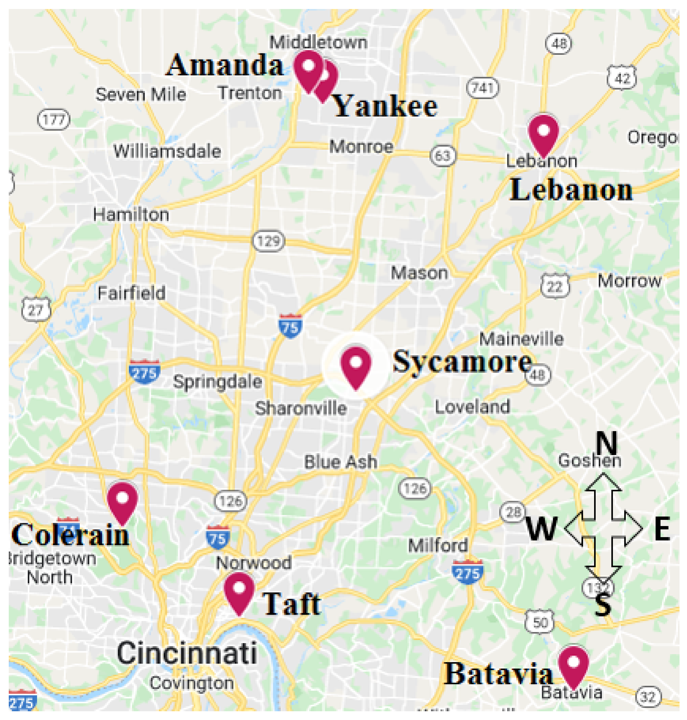
The present work quantifies the spatiotemporal variation of daily (24 h average) PM${}_{2.5}$ in the greater Cincinnati metropolitan area and PM${}_{2.5}$ sensitivities to meteorological parameters. Five years of PM${}_{2.5}$ and meteorological data were collected from the EPA CSN network and the North American Regional Reanalysis (NARR), respectively. The study area includes seven sites (Amanda, Batavia, Colerain, Lebanon, Sycamore, Taft, and Yankee) that measure PM${}_{2.5}$ using continuous monitors (Figure 1). A unique contribution from this work is that meteorology can be grouped by k-means clustering as opposed to seasons. We also evaluated the applicability to fit PM${}_{2.5}$ using the gamma distribution [32,33]. Principal components analysis (PCA) was used to determine the most important meteorological parameters for use in multivariate regression, which was used to quantify PM${}_{2.5}$ sensitivities to the local meteorology in Cincinnati. This work lays the foundation to develop PM${}_{2.5}$ forecast models using the techniques developed in this work.

2. Materials and Methods

2.1. Meteorological Data

Daily 24-h mean meteorological data were obtained using the North American Regional Reanalysis (NARR). The data consists of the following meteorological parameters for five years from August 2011 to December 2015: wind direction (WD), wind speed (WS), solar radiation (SR), relative humidity (RH), outdoor temperature (OT, K), visibility (VIS, km), planetary boundary height (HPBL, m), precipitation rate (PRATE, kg/m${}^2$/s), accumulated total precipitation (APCP, kg/m${}^2$), barometric pressure (BP, Pa), UWND.10 m’: Horizontal-wind speed at 10 m (m/s), VWND.10 m’: Vertical-wind at 10 m (m/s). The NARR dataset covers the entire study area, and as a result all sites in the study use the same meteorological data.

2.2. Continuous Particulate Matter Data Completeness

Hourly PM${}_{2.5}$ data from August 2011 to December 2015 (1797 days) were obtained from the Southwest Ohio Air Quality Agency (SWOAQA) and processed to remove negative and unreported values for all seven monitoring sites. In addition, days with less than 75% hourly data were considered incomplete and also removed. The processed data resulted in 958 days for which data were available for all seven sites.

2.3. Study Sites

The monitoring network is spread across five counties: Hamilton, Butler, Clermont, Clinton, and Warren, which constitute the five-county Cincinnati metropolitan area (Figure 1). The monitoring network consists of 18 sites, out of which seven operate three types of continuous PM${}_{2.5}$ samplers (

Table 1. Details of monitoring sites.

Site	Address	Latitude	Longitude	Sampler Type	Locality
Amanda	1300 Oxford Rd Middletown	39.478849	−84.407675	SHARP	Residential
Batavia	2400 Clermont Dr Batavia	39.0828	−84.1441	TEOM	Residential
Colerain	6950 Ripple Rd Cleves, Colerain	39.21487	−84.366192	MetONE BAM	Residential
Lebanon	416 Southeast St Lebanon	39.4293	−84.2006	MetONE BAM	Residential
Sycamore	11,590 Grooms Rd Sycamore	39.2787	−84.366192	SHARP	Residential
Taft	250 Taft Rd Cincinnati	39.123841	−84.504011	SHARP	Residential
Yankee	3350 Yankee Rd Middletown	39.472436	−84.394952	SHARP	Industrial

). These sites are operated and maintained by the SWOAQA and follow monitoring protocols established by the USEPA. The instruments used are the Tapered Element Oscillating Microbalance (TEOM), the Met-One Beta Attenuation Mass Monitor (BAM), and the Synchronized Hybrid Ambient Real Time Particulate (SHARP) monitors, which are all accepted as federal equivalent methods (FEMs). The TEOM is very sensitive to the ambient relative humidity, which causes a change in its oscillation frequency and can lead to both positive and negative artifacts [34]. Batavia uses a TEOM to collect concentrations and is more susceptible to error than instruments using beta-attenuation. BAM works on the principle of beta ray attenuation to measure airborne particulate concentration, and therefore the instrumental error is minimal. SHARP combines the speed of light scattering nephelometry with the accuracy of beta attenuation technology for continuous ${\mathrm{PM}}_{10}$ and PM${}_{2.5}$ measurements.

2.4. Clustering Analysis- K-Means Clustering

Clustering is a technique used to separate data into similar groups. Clustering methods vary depending on the distance measure, cluster evaluation criteria, and data type (real or binary data). Commonly used clustering principles are centroid-based, hierarchical, density-based, and graph-based clustering. A variety of distance measures, such as variants of Euclidean distance, Manhattan distance, Mahalanobis distance, cosine distance, and correlation measure can be used in determining the similarity of the data samples. Different cluster evaluation metrics include sum of squared error (SSE), cohesion, and entropy.

In this work, K-means, a widely used center-based clustering algorithm, was chosen. Euclidean distance and SSE were used to determine the similarity of data and evaluate clusters, respectively. K-means determines the members of a cluster such that the members have minimum Euclidean distances from the cluster center, relative to the other cluster centers. A heuristic-based method known as the elbow method was used to determine the optimal number of clusters [35,36]. K-means clustering was applied to the NARR data set using the “kmeans ()” function in Matlab (Mathworks, 2019).

2.5. Distribution Fitting: Lognormal vs. Gamma

Air pollution data are assumed to be lognormally distributed. However, it has been suggested that uncertainties of source impacts quantified by source apportionment models follow an inverse gamma distribution [37]. Here, we evaluated the use of fitting PM${}_{2.5}$ data using the gamma distribution, given that the gamma, like the lognormal, can be used to fit data with right tailed distributions. The Kolmogorov–Smirnov (KS) test is one such method that compares the maximum separation between the experimental cumulative frequency ($S_n\left(x\right)$) and the CDF of an assumed theoretical distribution ($F_X\left(x\right)$). It quantifies a critical value to determine how well the underlying data distribution matches the target distribution [38]. The limitation of the KS test is that the determination of the critical value is distribution-free. The null hypothesis is satisfied if $D_n<$ $D_n^{\alpha }$ where $D_n^{\alpha }$ is the critical value at the 5% significance level.

$$D_n=\underset{x}{max}\left|F_X\left(x\right)-S_n\left(x\right)\right|$$

(1)

In this work, PM${}_{2.5}$ data for the entire data set for four clusters and seasons were fitted to lognormal and gamma distributions, and the KS-Test was applied to check the satisfiability of the null hypothesis. The null hypothesis is satisfied if the computed KS statistic is less than the critical value.

2.6. Principal Component Analysis

PCA is a method that is often used to reduce the dimensionality of large datasets, by transforming a multidimensional data matrix into orthogonal components. The first step in PCA is to standardize the data matrix so that all variables have a mean of 0 and standard deviation of 1. Singular value decomposition is applied next to determine the principal components that are the eigenvectors of the dispersion matrix. The eigenvectors are orthonormal, and the resulting Z scores are orthogonal, which has the net effect of removing collinearity within the data matrix [31].

2.7. Multiple Linear Regression

Multiple linear regression is used to model a relationship between two or more predictor variables and a response variable by fitting a linear equation to the observed data. In this work, meteorological parameters used to predict PM${}_{2.5}$ (response variable) were determined using PCA results.

3. Results and Discussions

3.1. Spatial Variability

The Pearson’s correlation coefficient r for all possible pairs (21 pairs) of the given sites ranges between $0.62$ and $0.88$ (

Table 2. Correlation of PM${}_{2.5}$ across the monitoring sites.

Sites	Taft	Amanda	Batavia	Colerain	Lebanon	Sycamore	Yankee
Taft		0.84	0.72	0.88	0.87	0.88	0.82
Amanda			0.62	0.83	0.79	0.87	0.88
Batavia				0.65	0.68	0.67	0.63
Colerain					0.85	0.82	0.79
Lebanon						0.82	0.75
Sycamore							0.84

). The slope for the linear correlation can be found in the SI (Table S27). The lower correlations between Batavia and other sites are most likely due to the use of TEOM. However, even at the highly correlated sites (r = $0.88$, $r^2$ = $0.77)$, $23\%$ of PM${}_{2.5}$ variability could plausibly be attributed to local sources of air pollution.

3.2. PM${}_{2.5}$ Trends

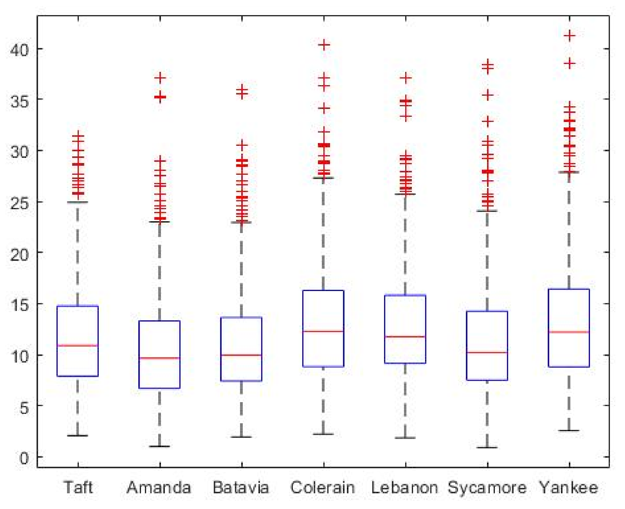
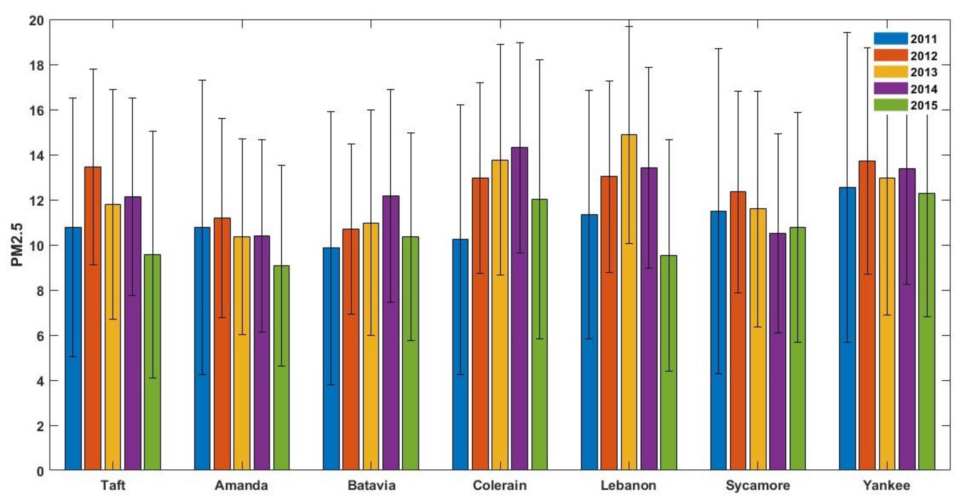
A boxplot of daily averages of PM${}_{2.5}$ is shown in Figure 2. The yearly average PM${}_{2.5}$ concentrations for different sites are detailed in

Table 3. Yearly averages of PM${}_{2.5}$.

Sites	Taft	Amanda	Batavia	Colerain	Lebanon	Sycamore	Yankee	Avg
2011	10.78 ± 5.74	10.76 ± 6.53	9.85 ± 6.07	10.23 ± 5.99	11.33 ± 5.51	11.50 ± 7.21	12.55 ± 6.87	11
2012	13.46 ± 4.34	11.19 ± 4.42	10.70 ± 3.78	12.96 ± 4.23	13.03 ± 4.25	12.34 ± 4.48	13.73 ± 5.02	12.49
2013	11.79 ± 5.11	10.36 ± 4.35	10.98 ± 4.99	13.76 ± 5.11	14.87 ± 4.80	11.60 ± 5.23	12.97 ± 6.08	12.33
2014	12.12 ± 4.38	10.40 ± 4.26	12.17 ± 4.70	14.31 ± 4.66	13.41 ± 4.46	10.51 ± 4.42	13.36 ± 5.104	12.33
2015	9.57 ± 5.48	9.08 ± 4.46	10.36 ± 4.59	12.02 ± 6.18	9.53 ± 5.14	10.76 ± 5.09	12.27 ± 5.45	10.51

, and the yearly variations are shown in Figure 3. The yearly average PM${}_{2.5}$ concentrations across years range between 9.08 $\mathsf{\mu }$g/m${}^3$ to 14.87 $\mathsf{\mu }$g/m${}^3$, and the overall mean is 11.73 $\mathsf{\mu }$g/m${}^3$. In 2011, Yankee had the highest PM${}_{2.5}$ among all the sites. However, all the sites in 2011 had a lower PM${}_{2.5}$ concentrations when compared to 2012, 2013, and 2014. In 2012, the average PM${}_{2.5}$ concentration was highest at Taft, Lebanon, and Yankee when compared to the other sites (Table 3). In 2013 and 2014, the highest PM${}_{2.5}$ concentration was observed in Lebanon and Colerain, respectively. The average concentrations across sites was highest in 2012, and the average across years was seen to be highest at Yankee. All sites showed a reduction in PM${}_{2.5}$ concentrations from 2013 through 2015. PM${}_{2.5}$ concentrations were lowest in 2015 for all the sites from the implementation of national and local control policies and more stringent PM${}_{2.5}$ NAAQS standards. National policies include controls for mobile sources (TIER 2 emissions standards, US EPA Diesel Rule, US EPA Clean Air Non-road Air Non-Road Diesel Rule, and the continued use of low sulfur gasoline and diesel) and stationary sources (Clean Air Interstate Rule for control of ${\mathrm{SO}}_2$ and ${\mathrm{NO}}_x$ emissions). Local controls include the implementation of policies from the Ohio State Implementation Plan, Diesel Emission Reduction Grant program, as well as permitting, enforcement, and compliance from the Southwest Ohio Air Quality Agency [39].

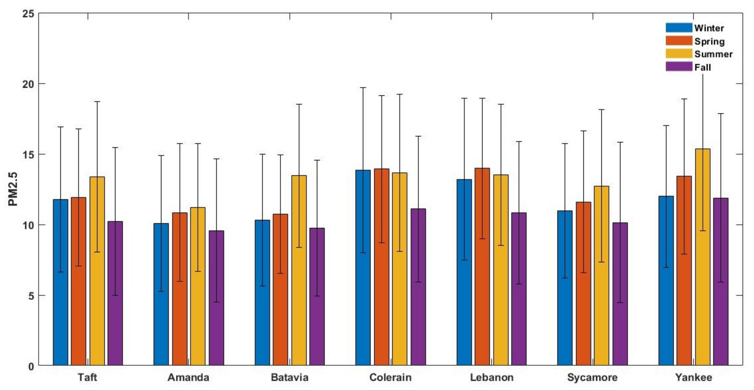
The average PM${}_{2.5}$ concentration across all the sites is highest in summer, followed by spring, winter, and fall (Figure 4,

Table 4. Seasonal averages of PM${}_{2.5}$.

Sites	Winter	Spring	Summer	Fall
Taft	11.75 ± 5.14	11.89 ± 4.86	13.36 ± 5.33	10.20 ± 5.23
Amanda	10.07 ± 4.81	10.84 ± 4.89	11.20 ± 4.53	9.57 ± 5.08
Batavia	10.33 ± 4.67	10.73 ± 4.18	13.45 ± 5.074	9.74 ± 4.82
Colerain	13.84 ± 5.83	13.93 ± 5.22	13.66 ± 5.57	11.10 ± 5.16
Lebanon	13.20 ± 5.74	13.98 ± 4.98	13.53 ± 5.00	10.82 ± 5.05
Sycamore	10.98 ± 4.77	11.60 ± 5.02	12.72 ± 5.40	10.13 ± 5.68
Yankee	11.99 ± 5.03	13.40 ± 5.51	15.35 ± 5.80	11.884 ± 5.96
MeanPM${}_{2.5}$	11.74	12.41	13.32	10.49

). The seasonal average of meteorological parameters are listed in

Table 5. Seasonal average of meteorological parameters.

Meteorology	Winter	Spring	Summer	Fall
WD	204.01	207.49	207.95	208.22
WS	1.49	1.47	1.05	1.33
RH	63.77	57.85	63.42	63.72
SR	60.78	143.02	194.20	98.96
BP (Pa)	736.62	737.13	737.09	737.74
OT (K)	274.81	285.50	297.93	286.51
APCP (kg/m${}^2$)	2.56	3.47	3.51	3.34
HPBL (m)	767.54	886.63	878.33	812.72
PRATE (kg/m${}^2$/s)	0.000027	0.000038	0.000041	0.000037
UWND.10 m (m/s)	1.73	0.84	0.93	0.99
VIS	16,363.58	17,549.05	18,751.20	18,027.20
VWND.10 m (m/s)	0.85	0.79	0.87	0.93

. Among all the sites, Yankee reports the highest PM${}_{2.5}$ (15.35 $\mathsf{\mu }$g/m${}^3$) in summer. However, the PM${}_{2.5}$ concentrations in Colerain in spring (13.93 $\mathsf{\mu }$g/m${}^3$) and winter (13.84 $\mathsf{\mu }$g/m${}^3$) are higher than summer. Likewise, the PM${}_{2.5}$ concentration in Lebanon in spring is higher than summer (Table 4). Spring experiences warmer days than winter, and both spring and winter experience cooler nights, which is favorable for inversions. The average PM${}_{2.5}$ in fall is relatively low compared to other seasons for all the sites.

3.3. Clustering Analysis at the Study Sites

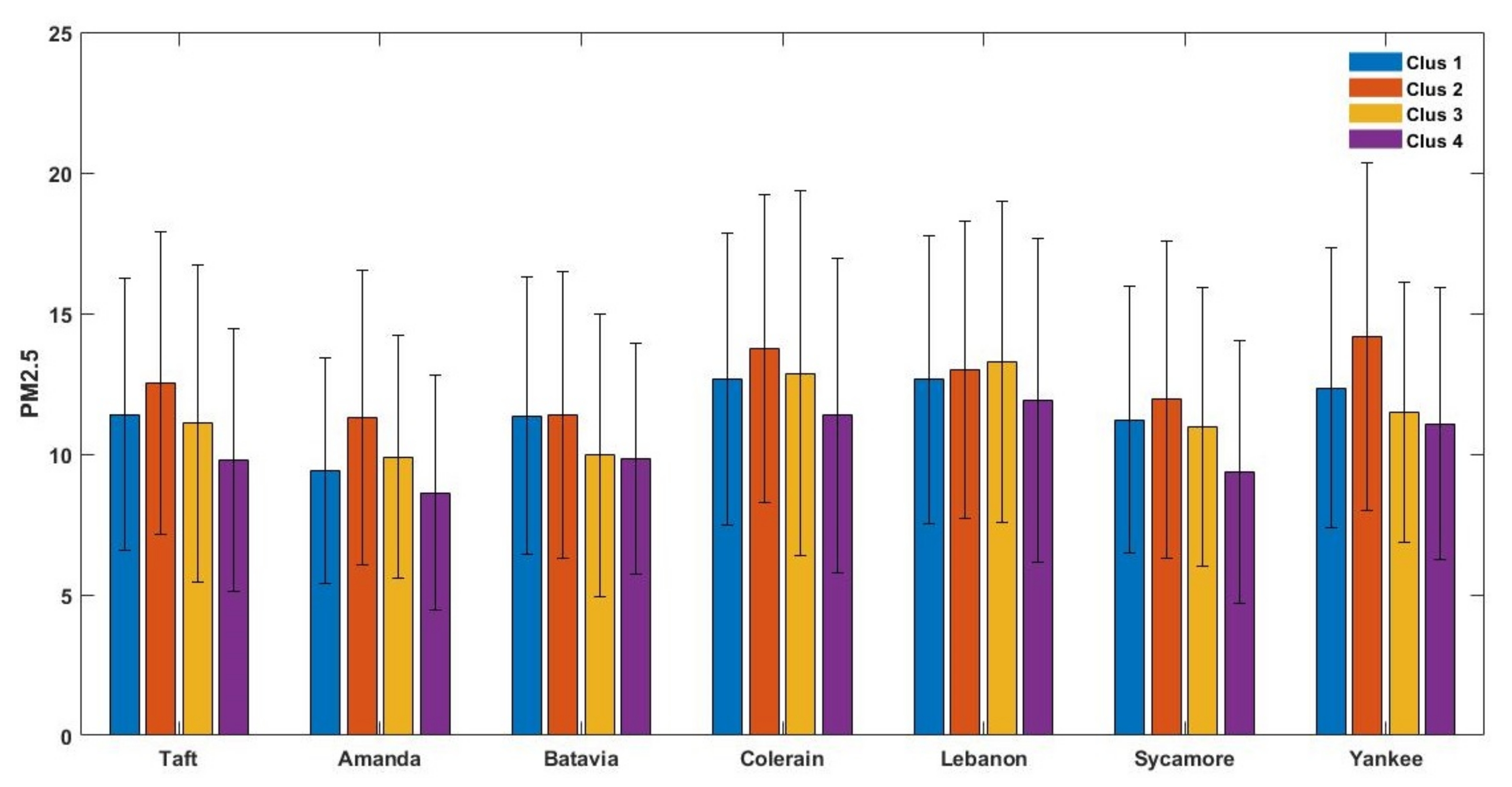
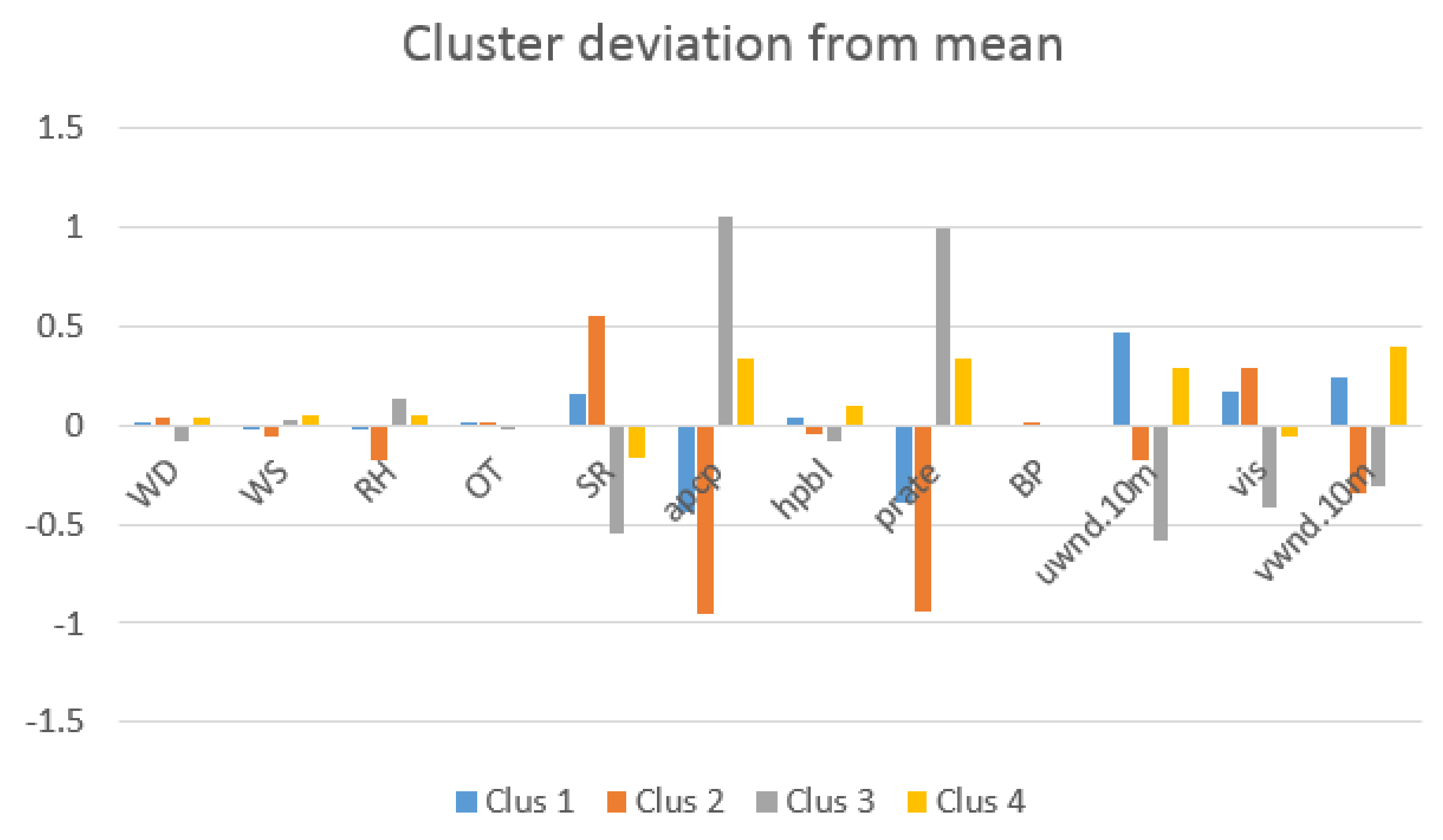
The cluster variation across all the seven sites are shown in Figure 5. Clustering using the elbow method resulted in four clusters. Of the total of 958 days, the majority of days were in C2 (528 days), followed by C1 (195 days), C4 (147 days), and C3 (88 days). All four clusters have days in all seasons (

Table 6. Mapping clusters onto seasons.

Cluster	Season	Days	Total
	Winter	61
C1	Spring	28	195
(warmer and drier days)	Summer	58
	Fall	48
	Winter	107
C2	Spring	115	528
(warmer and drier days)	Summer	146
	Fall	160
	Winter	50
C3	Spring	20	88
(cooler and wetter days)	Summer	2
	Fall	16
	Winter	48
C4	Spring	33	147
(cooler and wetter days)	Summer	25
	Fall	41

). C1 is comprised of 61 days in winter, 28 in spring, 58 in summer, and 48 in fall. C1 is characterized by moderate SR ($110.21$) and low PRATE ($0.00004$), which represents warmer and drier days, often seen throughout the year (

Table 7. PM${}_{2.5}$ Cluster averages at the study sites.

Sites	C1	C2	C3	C4
TPM${}_{2.5}$	11.41 ± 4.82	12.53 ± 5.39	11.10 ± 5.63	9.79 ± 4.65
APM${}_{2.5}$	9.41 ± 3.99	11.30 ± 5.25	9.90 ± 4.33	8.63 ± 4.18
BPM${}_{2.5}$	11.35 ± 4.93	11.41 ± 5.09	9.97 ± 5.03	9.83 ± 4.10
CPM${}_{2.5}$	12.65 ± 5.19	13.74 ± 5.48	12.87 ± 6.48	11.38 ± 5.58
LPM${}_{2.5}$	12.65 ± 5.13	13.01 ± 5.29	13.29 ± 5.70	11.91 ± 5.74
SPM${}_{2.5}$	11.22 ± 4.75	11.95 ± 5.64	10.96 ± 4.95	9.36 ± 4.66
YPM${}_{2.5}$	12.35 ± 4.97	14.17 ± 6.19	11.49 ± 4.64	11.08 ± 4.82
WD	206.54	209.71	186.16	209.57
WS	1.35	1.29	1.41	1.45
RH	66.55	56.06	76.80	71.34
SR	110.21	148.40	43.58	79.54
BP (Pa)	736.38	738.46	734.09	735.28
OT (K)	286.53	285.84	278.54	283.89
APCP (kg/m${}^2$)	3.34	0.30	12.22	7.92
HPBL (m)	870.49	801.28	769.91	920.91
PRATE (kg/m${}^2$/s)	0.000040	0.0000037	0.0001305	0.00009
UWND.10 m (m/s)	1.70	0.96	0.49	1.51
VIS	17,943.22	19,834.98	9043.51	14,526.51
VWND.10 m (m/s)	1.20	0.64	0.67	1.35

and Figure 6).

C2 has 146 days in summer, 160 days in fall, 115 spring days, and 107 days in winter. C2 is characterized by high solar radiation ($148.39$), low APCP (0.30 $\mathsf{\mu }$kg/m${}^2$), and low PRATE (0.0000037 $\mathsf{\mu }$kg/m${}^2$) (Table 7) and is consistent with the conditions usually observed in summer and the beginning of fall and represents warmer and drier days. C3 has 2 days in summer, 50 days in winter, 20 days in spring, and 16 days in fall. C3 is driven by low VIS (9043), low SR ($43.58$), high APCP (12.22 $\mathsf{\mu }$kg/m${}^2$), and high PRATE (0.000135 $\mathsf{\mu }$kg/m${}^2$/s), which represents cool and wetter days (Figure 6). C4 has 48 days in winter, followed by 41 days in fall, 33 days in spring, and 25 days in summer and also represents cooler days. C4 is driven by low SR ($79.54$), low VIS ($\mathrm{14,526.51}$), and moderately high APCP and PRATE (Figure 5). The wind directions predominantly come from the SSW direction for all four clusters.

Clustering allows viewing similar weather conditions from a multidimensional perspective, rather than temperature alone, the most defining feature of seasonality. The coefficient of variation (COV) of PM${}_{2.5}$ (the ratio of standard deviation for each cluster and season to the mean of each cluster and season, respectively) ranges from $0.39$ to $0.50$ across clusters and from $0.37$ to $0.53$ across seasons. The variation within clusters is similar to the variation within seasons (

Table 8. Coefficient of Variation.

	TPM${}_{2.5}$	APM${}_{2.5}$	BPM${}_{2.5}$	CPM${}_{2.5}$	LPM${}_{2.5}$	SPM${}_{2.5}$	YPM${}_{2.5}$	Mean	Stdev
C1	0.42	0.42	0.43	0.41	0.41	0.42	0.40	0.42	0.011
C2	0.43	0.46	0.45	0.40	0.41	0.47	0.44	0.44	0.02
C3	0.51	0.44	0.50	0.50	0.43	0.45	0.40	0.46	0.04
C4	0.47	0.48	0.42	0.49	0.48	0.50	0.43	0.47	0.03
Winter	0.44	0.48	0.45	0.42	0.44	0.43	0.42	0.44	0.02
Spring	0.41	0.45	0.39	0.37	0.36	0.43	0.41	0.40	0.03
Summer	0.40	0.40	0.38	0.41	0.37	0.42	0.38	0.39	0.01
Fall	0.51	0.53	0.49	0.46	0.47	0.56	0.50	0.50	0.03

) suggesting that clustering could potentially be a useful way to bin PM${}_{2.5}$ data based on meteorology. Given this similarity in $\left(COV\right)$, clustering could possibly offer a new way to develop forecast models.

3.4. Distribution Fitting: Lognormal vs. Gamma

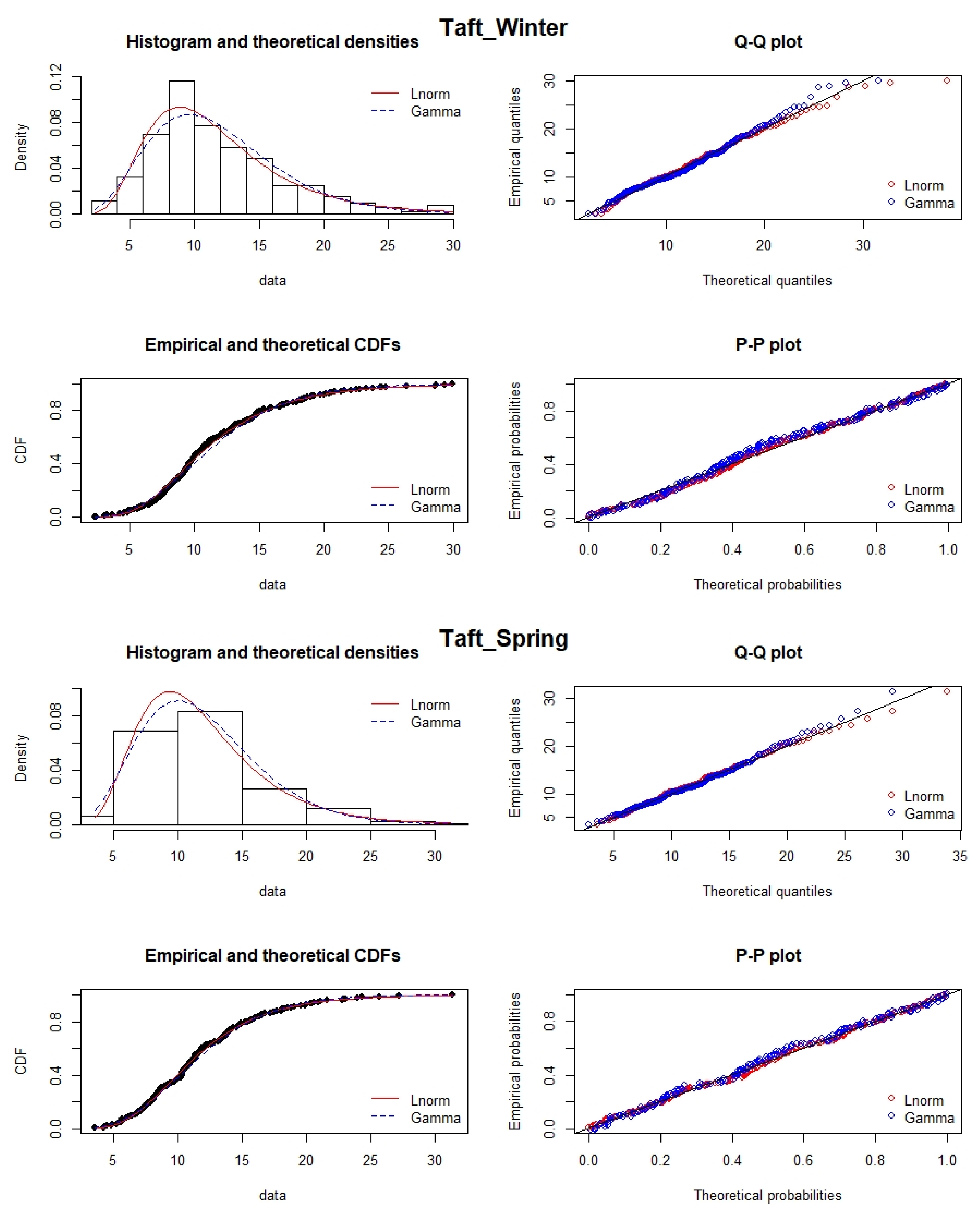
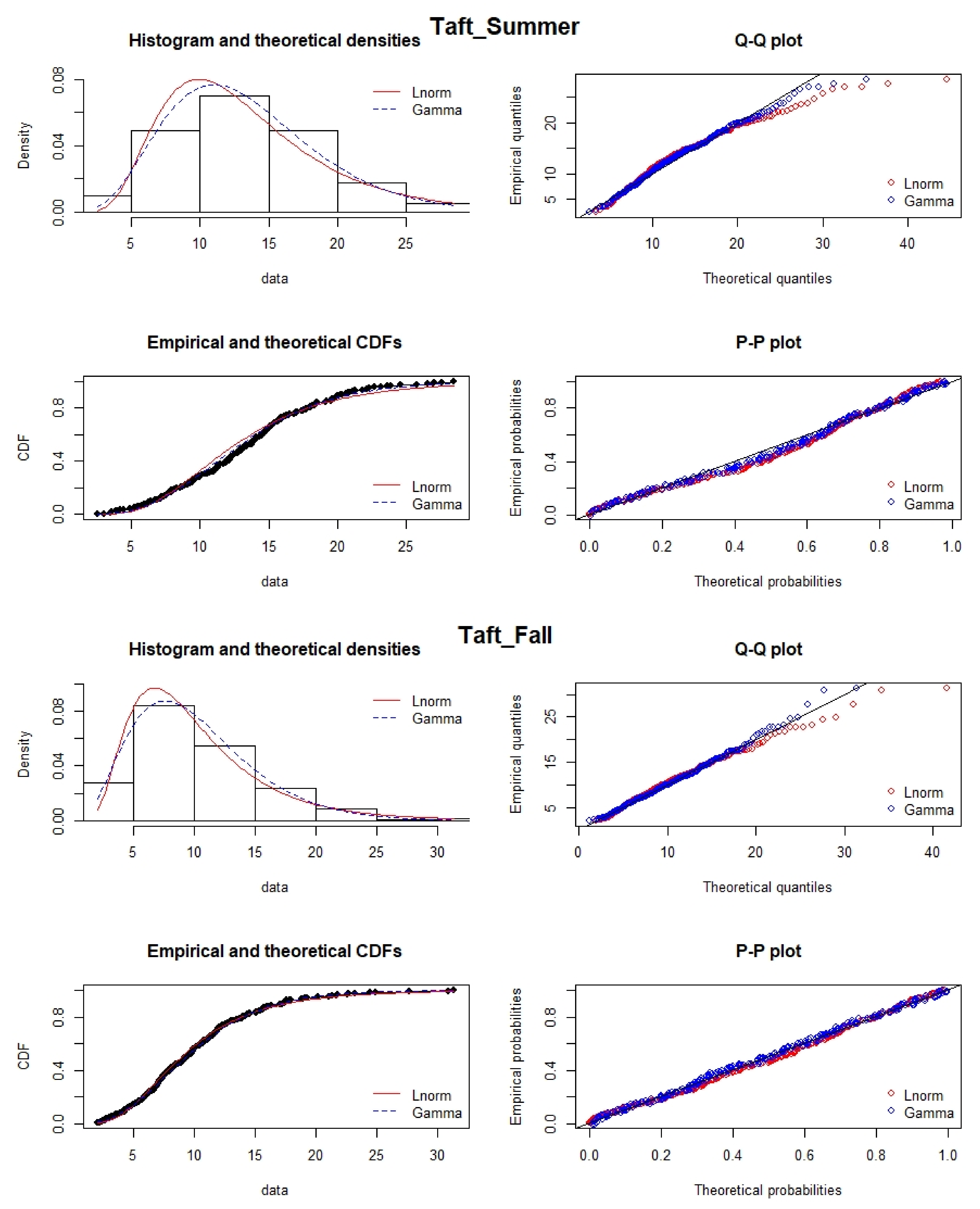
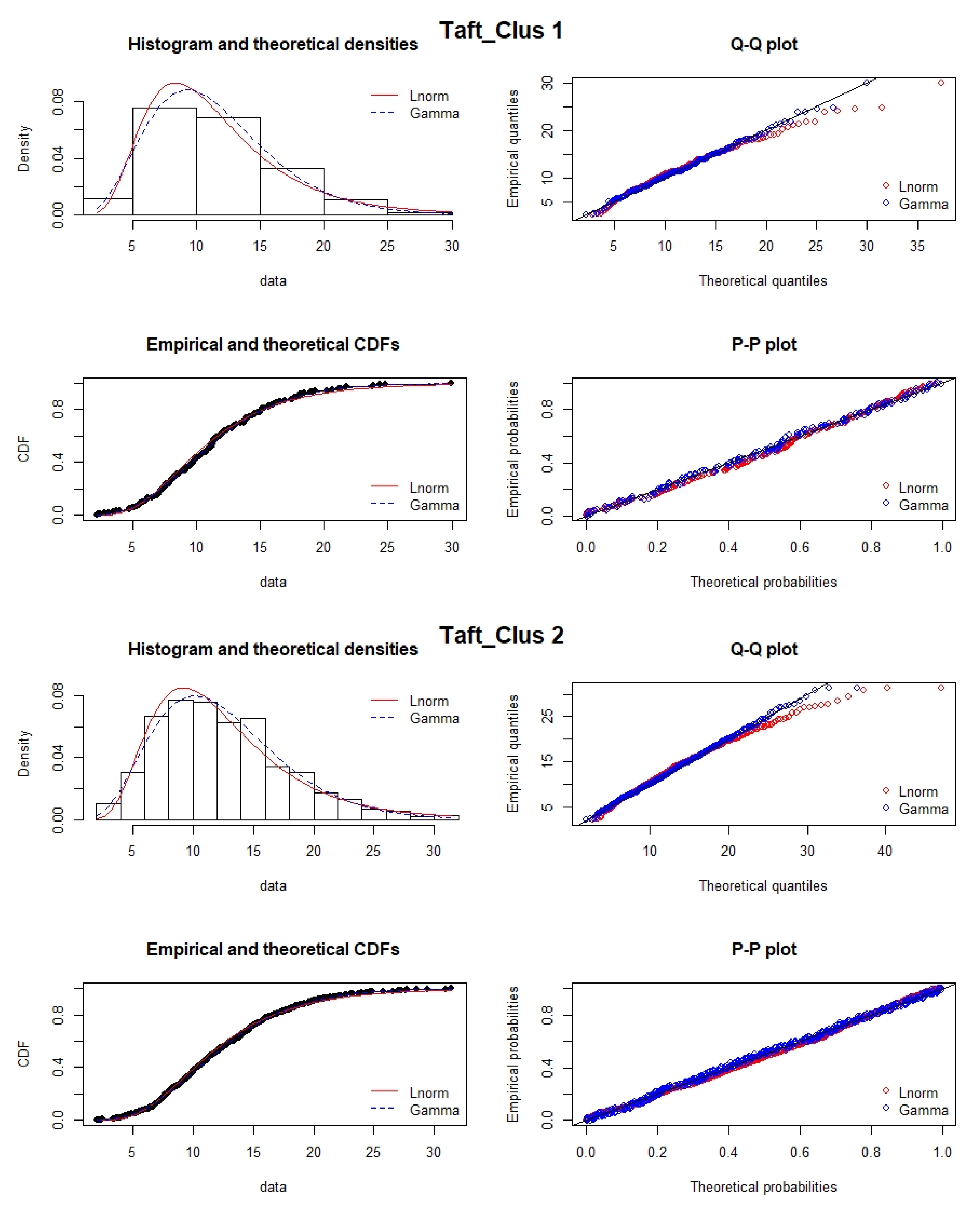
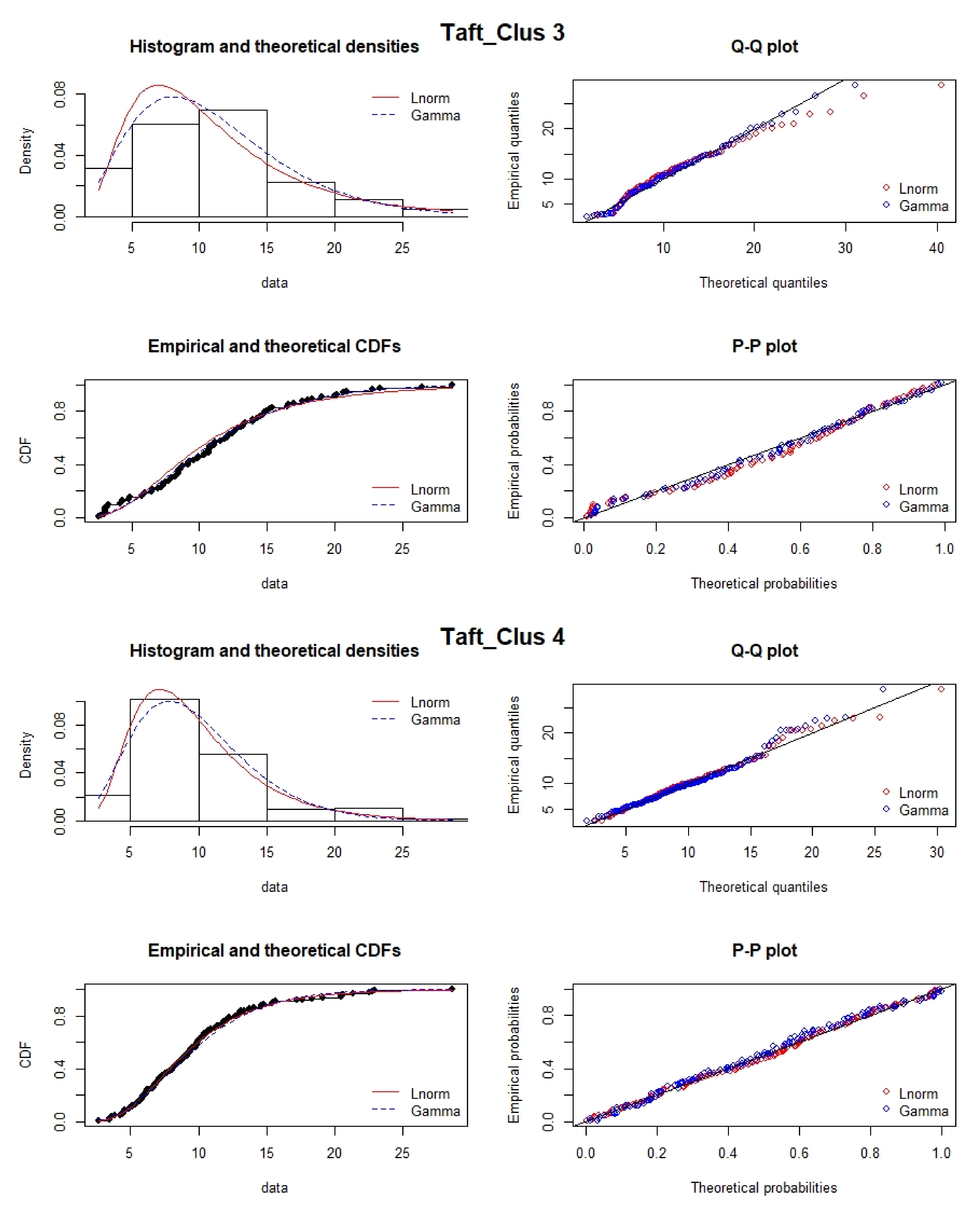
PM${}_{2.5}$ data for both the clusters and seasons were fit by the lognormal and gamma distributions at a 95% confidence interval ($\alpha$ = 0.05). Goodness of fit was tested using the Kolmogorov–Smirnov (KS) test. All clusters and seasons for all seven sites did not reject the null hypothesis for KS test with the only exception of summer at Taft where it rejects the null hypothesis for the lognormal distribution. Although both the distributions performed equally well, the gamma distribution, in general, had higher p-values than the lognormal suggesting a slightly higher confidence interval for the gamma distribution for the clusters and seasons (

Table 9. Fitting statistics for seasonal-based lognormal and gamma distributions.

	Lognormal		Gamma
Amanda	p-Value	KS Stat	p Value	KS Stat
winter	0.94	0.03	0.89	0.03
spring	0.16	0.07	0.62	0.05
summer	0.18	0.07	0.36	0.05
fall	0.77	0.03	0.99	0.02
Batavia
winter	0.81	0.03	0.25	0.06
spring	0.83	0.04	0.48	0.05
summer	0.35	0.06	0.72	0.04
fall	0.79	0.03	0.59	0.04
Colerain
winter	0.50	0.04	0.71	0.04
spring	0.93	0.03	0.97	0.03
summer	0.15	0.07	0.48	0.05
fall	0.50	0.04	0.40	0.05
Lebanon
winter	0.09	0.07	0.26	0.06
spring	0.44	0.06	0.81	0.04
summer	0.50	0.05	0.77	0.04
fall	0.47	0.05	0.35	0.05
Sycamore
winter	0.85	0.03	0.34	0.05
spring	0.69	0.04	0.91	0.03
summer	0.33	0.06	0.40	0.05
fall	0.69	0.04	0.92	0.03
Taft
winter	0.53	0.04	0.17	0.06
spring	0.63	0.05	0.65	0.05
summer	0.04	0.08	0.35	0.06
fall	0.53	0.04	0.96	0.02
Yankee
winter	0.84	0.03	0.46	0.05
spring	0.45	0.05	0.87	0.04
summer	0.29	0.06	0.80	0.04
fall	0.78	0.03	0.90	0.03

and

Table 10. Fitting statistics for clustering based lognormal and gamma distributions.

	Gamma		Lognormal
Amanda	p-Value	KS Stat	p Value	KS Stat
C1	0.99	0.02	0.73	0.04
C2	0.35	0.03	0.12	0.05
C3	0.73	0.07	0.33	0.09
C4	0.95	0.04	0.46	0.06
Batavia
C1	0.33	0.06	0.84	0.04
C2	0.17	0.04	0.88	0.02
C3	0.55	0.08	0.75	0.06
C4	0.96	0.03	0.49	0.06
Colerain
C1	0.95	0.03	0.73	0.04
C2	0.94	0.02	0.17	0.04
C3	0.97	0.04	0.60	0.07
C4	0.82	0.05	0.95	0.04
Lebanon
C1	0.49	0.05	0.11	0.08
C2	0.85	0.02	0.59	0.03
C3	0.69	0.07	0.25	0.10
C4	0.38	0.07	0.17	0.08
Sycamore
C1	0.75	0.04	0.97	0.03
C2	0.26	0.04	0.79	0.02
C3	0.51	0.08	0.35	0.09
C4	0.91	0.04	0.59	0.06
Taft
C1	0.97	0.03	0.49	0.05
C2	0.98	0.01	0.37	0.03
C3	0.84	0.06	0.42	0.09
C4	0.72	0.05	0.97	0.03
Yankee
C1	0.97	0.03	0.95	0.03
C2	0.68	0.03	0.12	0.05
C3	0.76	0.06	0.36	0.09
C4	0.98	0.03	0.79	0.05

). A comparison between the gamma and lognormal distributions shows that both the PDFs give similar results for daily PM${}_{2.5}$ concentrations from seven sites in Cincinnati, during all seasons and for four clusters (Supplementary Materials Figures S1–S48 and Tables S1–S27). Figure 7 and Figure 8 shows the PDFs and Q-Q plots for the Taft site. The Q-Q plots show that the gamma distribution captures higher concentrations better than the lognormal. As air quality continues to improve, these days with relatively high PM${}_{2.5}$ concentrations are expected to play an important role in developing future air quality management strategies.

3.5. Principal Component Analysis

The first five PCs cumulatively explained more than 80% of the total variance, and the total variance explained by each principal component was 31.97, 16.97, 16.17, 8.64, and 7.80 for PC1 to PC5, respectively. The loadings greater than $\pm 0.3$ are highlighted in bold, and in this work they are assumed to be the most significant parameters and interactions within each PC. The first principal component consists mainly of positive contributions from RH, APCP, and PRATE and negative contributions from VIS (

Table 11. The total variance explained by each principal component: Taft.

Meteorology	PC1	PC2	PC3	PC4	PC5	PC6	PC7	PC8	PC9	PC10	PC11	PC12
WS	0.04	0.03	−0.49	0.19	−0.09	−0.54	0.38	0.07	−0.33	−0.11	0.78	0.007
RH	0.37	−0.18	0.16	−0.21	0.00	0.14	0.37	−0.48	−0.08	−0.18	0.58	−0.06
BP	−0.33	−0.29	0.13	0.31	0.32	0.13	0.36	−0.01	−0.03	−0.14	−0.18	−0.63
SR	−0.24	0.36	0.36	0.14	−0.15	−0.01	0.19	0.53	0.08	0.04	0.56	−0.03
OT	0.05	0.37	0.53	−0.08	0.02	−0.12	0.37	−0.13	−0.19	−0.22	−0.48	0.28
APCP	0.40	−0.03	0.20	0.43	0.09	−0.05	−0.19	0.03	−0.18	0.16	0.01	0.02
HPBL	0.13	0.44	−0.25	0.38	0.11	0.08	0.24	−0.30	0.63	0.14	−0.03	0.03
PRATE	0.39	−0.02	0.21	0.44	0.10	−0.04	−0.19	0.03	−0.22	0.16	0.03	−0.08
UWIND.10 m	0.05	0.32	−0.38	0.05	0.18	0.65	0.11	0.15	−0.48	−0.11	0.01	0.10
VIS	−0.37	0.25	0.06	−0.12	0.16	−0.12	−0.04	−0.41	−0.33	0.66	0.12	−0.10
VWIND.10 m	0.16	0.22	−0.01	−0.32	0.79	−0.27	−0.18	0.17	0.10	−0.18	0.12	−0.11

). The second component has positive contributions from SR, OT, and HPBL. The third component is dominated by WS, OT, SR, and UWND, the fourth and the fifth component by APCP, HPBL, PRATE, BP, VWND and VWND, BP, respectively.

3.6. Multiple Linear Regression

PM${}_{2.5}$ was regressed against meteorological parameters from the first five PCs that had loadings that met three threshold criteria: $\pm 0.3$ and $\pm 0.4$ and $\pm 0.44$ [40]. For the first and the second threshold ($\pm 0.3$ and $\pm 0.4$ respectively), these meteorological parameters were WS, RH, SR, OT, HPBL, APCP, PRATE and VIS. For the third threshold ($\pm 0.44$), the parameters selected were APCP, PRATE, OT, HPBL and WS. MLR was used over these two combinations of parameters. Although UWIND and VWIND both met the threshold criteria, they were not used in the MLR Runs since the total magnitude WS is the parameter of interest with regards to PM${}_{2.5}$ sensitivity. Using the first and second threshold (MLR Run 1) the meteorological parameters that are statistically significant at a p-value of 0.05 (95% confidence) were SR, HPBL, OT and VIS. Using the third threshold (MLR Run 2), the statistically significant parameters were HPBL and OT in the third threshold (MLR Run 2). When all meteorological parameters were used (MLR Run 3), the statistically significant parameters were BP, SR, HPBL, OT and VIS (

Table 12. MLR analysis at Taft.

MLR Runs	No.of Variables (p)	Predictor Variables	r	$r^2$
1	3	HPBL, OT, VIS	0.41	0.17
2	2	HPBL, OT,	0.40	0.16
3	4	BP, HPBL, OT, VIS	0.42	0.18

). The intercept for all the three MLR runs were not statistically significant. It should be noted that when SR was included in the regression, PM${}_{2.5}$ had a negative sensitivity to OT which is not consistent with the findings in literature. One plausible reason is that SR might be accounting for the effects of temperature. To address potential confounding, MLR was run again for the three combinations using only the meteorological parameters which were statistically significant and with SR removed. $r^2$ values for MLR Runs 1, 2 and 3 were 0.17 (three predictor variables), 0.16 (two predictor variables) and 0.18 (four predictor variables), respectively (Table 12).

MLR results are consistent across all three runs with PM${}_{2.5}$ having negative sensitivities to HPBL and BP and positive sensitivities to OT and VIS (

Table 13. PM${}_{2.5}$ sensitivities at Taft. SE represents standard error. The uncertainty of the average sensitivity was calculated using propagation of errors.

Meteorological	PM${}_{2.5}$ Sensitivity	PM${}_{2.5}$ Sensitivity	PM${}_{2.5}$ Sensitivity	Average	Uncertainty
Parameters	MLR Run 1 (SE)	MLR Run 2 (SE)	MLR Run 3 (SE)
HPBL	−6.76 $\mathsf{\mu }$g/m${}^3$/ (1000 m)	−6.89 $\mathsf{\mu }$g/m${}^3$/ (1000 m)	−6.82 $\mathsf{\mu }$g/m${}^3$/ (1000 m)
	(0.0005)	(0.0005)	(0.017)	−6.823	0.906
OT	0.05 $\mathsf{\mu }$g/m${}^3$/K	0.08 $\mathsf{\mu }$g/m${}^3$/K	0.07 $\mathsf{\mu }$g/m${}^3$/K
	(0.003)	(0.014)	(0.014)	0.068	0.021
VIS	0.15 $\mathsf{\mu }$g/m${}^3$/km	-	0.15 $\mathsf{\mu }$g/m${}^3$/km
	(0.00005)		(0.00004)	0.15	0.066
BP	-	-	−0.007/Pa
			0.0055

). Although other studies show a relationship to RH, in our work PM${}_{2.5}$ sensitivity to RH was not statistically significant. For example, Balachandran et al., (2017) showed that a 10% increase in daily average of RH would increase 0.27 $\mathsf{\mu }$g/m${}^3$ of PM${}_{2.5}$. Their work investigated the impact of prescribed fires whereas this work does not investigate specific emissions conditions. Tai et al. (2010) showed that temperature is positively correlated to PM${}_{2.5}$ concentrations throughout the US and RH is positively correlated to PM${}_{2.5}$ in the Northeast and Midwest but negatively correlated in the Southeast and West. Similarly, Leung et al. (2018) showed that PM${}_{2.5}$ has both positive (r = 0.4) and negative correlation (r = 0.4, 0.2) to RH, depending on location in China. This location specific nature of PM${}_{2.5}$ sensitivity to RH might be one plausible explanation for the lack of statistical significance in our work. For all three MLR runs, our results show that 1000 m increase in HPBL decreases PM${}_{2.5}$ by 6.8 $\mathsf{\mu }$g/m${}^3$. HPBL can act as a proxy for some of the cumulative effects of various meteorological phenomena such as transport by winds, temperature gradients, moisture content, and the dilution of pollution in the atmospheric boundary layer that impacts PM${}_{2.5}$ concentrations. PM${}_{2.5}$ shows a positive sensitivity to VIS (statistically significant in MLR Runs 1 and 2 only) and therefore a 1 km increase in VIS results in an increase of 0.15 $\mathsf{\mu }$g/m${}^3$ of PM${}_{2.5}$. PM${}_{2.5}$ has a positive sensitivity to OT and every 10K increase in temperature would increase PM${}_{2.5}$ by 0.7 $\mathsf{\mu }$g/m${}^3$, consistent with Leung et al. (2018), who showed that temperature has a positive correlation (r = 0.60) with PM${}_{2.5}$. However other work, such as Dawson et al. (2007), showed a negative sensitivity of PM${}_{2.5}$ to temperature of 0.016 and 0.17 $\mathsf{\mu }$g/m${}^3$/K in summer and winter, respectively. Finally, PM${}_{2.5}$ has a negative sensitivity to BP (statistically significant in MLR Run 3 only) and an increase of 100 Pa decreases PM${}_{2.5}$ by 0.7 $\mathsf{\mu }$g/m${}^3$

Our results show an $r^2$ of 0.17 when three predictor variables were used (MLR Run1), 0.16 with two predictor variable (MLR Run 2) and 0.18 with four variables (MLR run 3) Table 12. In Rui et al. (2018), the $r^2$ was 0.76 when gaseous pollutants, AOD and meteorological parameters were used. In Cifuentes et al. (2021), r values ranged from 0.16-0.27 when only meteorological parameters were used but increased to 0.41 when air pollutants are included with meteorology.

4. Conclusions

This work lays the foundation for a new way to understand relationships between air pollution and meteorology by analyzing the spatial and temporal variation of PM${}_{2.5}$ and its sensitivity to meteorological parameters in the greater Cincinnati area. A unique contribution from this work is that meteorology can be grouped using k-means clustering in addition to seasons. PM${}_{2.5}$ concentrations are moderately correlated across all sites (r = 0.62 − 0.84). Average PM${}_{2.5}$ concentrations are highest in summer for all sites, except for Colerain and Lebanon where PM${}_{2.5}$ concentrations are highest in spring. The coefficient of variation of average concentrations across all sites are similar when grouped by clusters as by seasons. Based on the KS test, the gamma distribution fits the PM${}_{2.5}$ slightly better than the lognormal, suggesting that modeling efforts can use the highly flexible gamma distribution. Although the relationship between the variables of the dataset is not linear, the use of PCA to guide the MLR allowed the use of a smaller subset of the meteorological parameters. RH, HPBL, APCP, OT, PRATE, WS, and VIS are the most important parameters in the first five principal components (which cumulatively explained greater than 80 percent of variance). MLR using two combinations of these parameters as well as all meteorological variables resulted in the following statistically significant parameters: HPBP, OT, VIS and BP. The $r^2$ value ranged from 0.16 and 0.17. Our future work will be to develop a PM${}_{2.5}$ forecast model with the help of artificial neural networks using clustering of meteorology as well as gamma distribution statistics.

References

- Garrett, P.; Casimiro, E. Short-term effect of fine particulate matter (PM2.5) and ozone on daily mortality in Lisbon, Portugal. Environ. Sci. Pollut. Res. 2011, 18, 1585–1592. [Google Scholar] [CrossRef] [PubMed]
- Lave, L.B.; Seskin, E.P. Air pollution and human health. Science 1970, 169, 723–733. [Google Scholar] [CrossRef] [PubMed] [Green Version]
- Ebenstein, A.; Fan, M.Y.; Greenstone, M.; He, G.J.; Zhou, M.G. New evidence on the impact of sustained exposure to air pollution on life expectancy from China’s Hua River Policy. Proc. Natl. Acad. Sci. USA 2017, 114, 10384–10389. [Google Scholar] [CrossRef] [PubMed] [Green Version]
- Li, L.L.; Tan, Q.W.; Zhang, Y.H.; Feng, M.; Qu, Y.; An, J.L.; Liu, X.G. Characteristics and source apportionment of PM2.5 during persistent extreme haze events in Chengdu, Southwest China. Environ. Pollut. 2017, 230, 718–729. [Google Scholar] [CrossRef]
- Dawson, J.P.; Bloomer, B.J.; Winner, D.A.; Weaver, C.P. Understanding the Meteorological Drivers of Us Particulate Matter Concentrations in a Changing Climate. Bull. Am. Meteorol. Soc. 2014, 95, 520–532. [Google Scholar] [CrossRef]
- Russell, A.G.; Brunekreef, B. A Focus on Particulate Matter and Health. Environ. Sci. Technol. 2009, 43, 4620–4625. [Google Scholar] [CrossRef] [PubMed] [Green Version]
- Giang, P.; Dung, D.; Giang, K.; Vinhc, H.; Rocklöv, J. The effect of temperature on cardiovascular disease hospital admissions among elderly people in Thai Nguyen Province, Vietnam. Glob. Health Action 2014, 7, 23649. [Google Scholar] [CrossRef] [Green Version]
- Kim, Y.J.; Kim, K.W.; Kim, S.D.; Lee, B.K.; Han, J.S. Fine particulate matter characteristics and its impact on VISibility impairment at two urban sites in Korea: Seoul and Incheon. Atmos. Environ. 2006, 40, S593–S605. [Google Scholar] [CrossRef]
- Abdul-Wahab, S.A.; Bakheit, C.S.; Al-Alawi, S.M. Principal component and multiple regression analysis in modelling of ground-level ozone and factors affecting its concentrations. Environ. Model. Softw. 2005, 20, 1263–1271. [Google Scholar] [CrossRef]
- Cheng, Y.F.; Zheng, G.J.; Wei, C.; Mu, Q.; Zheng, B.; Wang, Z.B.; Gao, M.; Zhang, Q.; He, K.B. Reactive nitrogen chemistry in aerosol water as a source of sulfate during haze events in China. Sci. Adv. 2016, 2, e1601530. [Google Scholar] [CrossRef] [Green Version]
- Wang, Z.; Pan, X.L.; Uno, I.; Li, J.; Wang, Z.F.; Chen, X.S.; Fu, P.Q.; Yang, T.; Kobayashi, H.; Shimizu, A.; et al. Signi ficant impacts of heterogeneous reactions on the chemical composition and mixing state of dust particles: A case study during dust events over northern China. Atmos. Environ. 2017, 159, 83–91. [Google Scholar] [CrossRef]
- Quan, J.N.; Tie, X.X.; Zhang, Q.; Liu, Q.; Li, X.; Gao, Y.; Zhao, D.L. Characteristics of heavy aerosol pollution during the 2012–2013 winter in Beijing, China. Atmos. Environ. 2014, 88, 83–89. [Google Scholar] [CrossRef]
- Xu, J.S.; Xu, H.H.; Xiao, H.; Tong, L.; Snape, C.E.; Wang, C.J.; He, J. Aerosol composition and sources during high and low pollution periods in Ningbo, China. Atmos. Res. 2016, 178–179, 559–569. [Google Scholar] [CrossRef]
- Chang, D.; Song, Y.; Liu, B. VISibility trends in six megacities in China 1973–2007. Atmos. Res. 2009, 94, 94161–94167. [Google Scholar] [CrossRef]
- Cao, Z.; Sheng, L.; Liu, Q.; Yao, X.; Wang, W. Interannual increase of regional haze-fog in North China plain in summer by intensi fied easterly winds and orographic forcing. Atmos. Environ. 2015, 122, 154–162. [Google Scholar] [CrossRef]
- Chen, W.; Tang, H.Z.; Zhao, H.M. Diurnal, weekly and monthly spatial variations of air pollutants and air quality of Beijing. Atmos. Environ. 2015, 119, 21–34. [Google Scholar] [CrossRef]
- Zhao, S.Y.; Zhang, H.; Xie, B. The effects of El Niño –southern oscillation on the winter haze pollution of China. Atmos. Chem. Phys. 2018, 18, 1863–1877. [Google Scholar] [CrossRef] [Green Version]
- Bi, J.; Huang, J.; Hu, Z.; Holben, B.N.; Guo, Z. Investigating the aerosol optical and radiative characteristics of heavy haze episodes in Beijing during January of 2013. J. Geophys. Res. Atmos. 2014, 119, 9884–9900. [Google Scholar] [CrossRef]
- Martuzevicius, D.; Luo, J.; Reponen, T.; Shukla, R.; Kelley, A.L.; StClair, H.; Grinshpun, S.A. Evaluation and optimization of an urban PM2.5 monitoring network. J. Environ. Monit. 2005, 7, 67–77. [Google Scholar] [CrossRef]
- Mar, T.F.; Norris, G.A.; Koenig, J.Q.; Larson, T.V. Associations between air pollution and mortality in Phoenix. Environ. Health Perspect. 2000, 108, 347–353. [Google Scholar] [CrossRef]
- Pinto, J.P.; Lefohn, A.S.; Shadwick, D.S. Spatial Variability of PM2.5 i Urban Areas in the United States. J. Air Waste Manag. Assoc. 2004, 54, 440–449. [Google Scholar] [CrossRef] [Green Version]
- Galindo, N.; Varea, M.; Gil-Moltó, J.; Yubero, E.; Nicolás, J. The Influence of Meteorology on Particulate Matter Concentrations at an Urban Mediterranean Location. Water Air Soil Pollut. 2011, 215, 365–372. [Google Scholar] [CrossRef]
- Liu, Z.; Shen, L.; Yan, C.; Du, J.; Li, Y.; Zhao, H. Analysis of the Influence of Precipitation and Wind on PM2.5 and PM10 in the Atmosphere. Adv. Meteorol. 2020, 2020, 5039613. [Google Scholar] [CrossRef]
- Yadav, R. The linkages of anthropogenic emissions and meteorology in the rapid increase of particulate matter at a foothill city in the Arawali range of India. Atmos. Environ. 2014, 85, 147–151. [Google Scholar] [CrossRef]
- Jacob, D.J.; Winner, D.A. Effect of climate change on air quality. Atmos. Environ. 2009, 43, 51–63. [Google Scholar] [CrossRef] [Green Version]
- Leung, D.M.; Tai, A.P.K.; Mickley, L.J.; Moch, J.M.; van Donkelaar, A.; Shen, L.; Martin, R.V. Synoptic meteorological modes of variability for fine particulate matter (PM2.5) air quality in major metropolitan regions of China. Atmos. Chem. Phys. 2018, 18, 6733–6748. [Google Scholar] [CrossRef] [Green Version]
- Tai, A.P.K.; Mickley, L.J.; Jacob, D.J. Correlations between fine particulate matter (PM2.5) and meteorological variables in the United States: Implications for the sensitivity of PM2.5 to climate change. Atmos. Environ. 2010, 44, 3976–3984. [Google Scholar] [CrossRef]
- Megaritis, A.G.; Fountoukis, C.; Charalampidis, P.E.; Denier van der Gon, H.A.C.; Pilinis, C.; Pandis, S.N. Linking climate and air quality over Europe: Effects of meteorology on PM2.5 concentrations. Atmos. Chem. Phys. 2014, 14, 10283–10298. [Google Scholar] [CrossRef] [Green Version]
- Camalier, L.; Cox, W.; Dolwick, P. The effects of meteorology on ozone in urban areas and their use in assessing ozone trends. Atmos. Environ. 2007, 41, 7127–7137. [Google Scholar] [CrossRef]
- Schlink, U.; Herbarth, O.; Richter, M.; Dorling, S.; Nunnari, G.; Cawley, G.; Pelikan, E. Statistical models to assess the health effects and to forecast ground-level ozone. Environ. Model. Softw. 2006, 21, 547–558. [Google Scholar] [CrossRef]
- Balachandran, S.; Baumann, K.; Pachon, J.E.; Mulholland, J.A.; Russell, A.G. Evaluation of fire weather forecasts using PM2.5 sensitivity analysis. Atmos. Environ. 2017, 148, 128–138. [Google Scholar] [CrossRef] [Green Version]
- Thom, H.C. A note on the gamma distribution. Mon. Weather 1958, 86, 117–122. [Google Scholar] [CrossRef]
- Husak, G.J.; Michaelsen, J.; Funk, C. Use of the gamma distribution to represent monthly rainfall in Africa for drought monitoring applications. Int. J. Climatol. 2007, 27, 935–944. [Google Scholar] [CrossRef]
- Li, Q.-F.; Wang, L.; Liu, Z.; Heber, A.J. Field evaluation of particulate matter measurements using tapered element oscillating microbalance in a layer house. J. Air Waste Manag. Assoc. 2012, 62, 322–335. [Google Scholar] [CrossRef] [Green Version]
- Liu, F.; Deng, Y. Determine the Number of Unknown Targets in Open World Based on Elbow Method. IEEE Trans. Fuzzy Syst. 2021, 29, 986–995. [Google Scholar] [CrossRef]
- Marutho, D.; Handaka, S.H.; Wijaya, E. The Determination of Cluster Number at k-mean using Elbow Method and Purity Evaluation on Headline News. In Proceedings of the 2018 International Seminar on Application for Technology of Information and Communication, Semarang, Indonesia, 21–22 September 2018. [Google Scholar]
- Balachandran, S.; Chang, H.H.; Pachon, J.E.; Holmes, H.A.; Mulholland, J.A.; Russell, A.G. Bayesian-Based Ensemble Source Apportionment of PM2.5. Environ. Sci. Technol. 2013, 47, 13511–13518. [Google Scholar] [CrossRef] [PubMed]
- Grall-Maës, E. Use of the Kolmogorov–Smirnov test for gamma process. J. Risk Reliab. 2012, 226, 624–634. [Google Scholar] [CrossRef]
- Available online: https://epa.ohio.gov/static/Portals/27/sip/eis/Final_SIP_PM25_Document.pdf (accessed on 9 March 2022).
- Binaku, K.; Schmeling, M. Multivariate statistical analyses of air pollutants and meteorology in Chicago during summers 2010–2012. Air Qual. Atmos. Health 2017, 10, 1227–1236. [Google Scholar] [CrossRef] [Green Version]
Figure 1.
Map of monitoring sites in Cincinnati. (Source: Google maps).
Figure 2.
Boxplot of daily averages of PM. The red line represents the median; the edges of the box are 25th and 75th percentiles; and the whiskers are the extreme data points. The edges of the dashed line represent the extremes that are not considered to be outliers.
Figure 3.
Yearly variation of PM at the monitoring sites. Error bars represent 1 standard deviation of variability in the time series.
Figure 4.
Seasonal variation of PM at the monitoring sites. Error bars represent 1 standard deviation of variability in the time series.
Figure 5.
Cluster variation of PM at the monitoring sites. Error bars represent 1 standard deviation of variability in the time series.
Figure 6.
Cluster deviation from mean.
Figure 7.
Comparison of Gamma and Lognormal distribution for Taft (central monitoring site) across four seasons (blue line represents gamma distribution and red represents lognormal).
Figure 8.
Comparison of Gamma and Lognormal distribution for Taft (central monitoring site) across four clusters (blue line represents gamma distribution and red represents lognormal).