Article

Verification by Multiple Methods of Precipitation Forecast from HDRFFGS and SisPI Tools during the Impact of the Tropical Storm Isaias over the Dominican Republic †

by
Maibys Sierra-Lorenzo
1,*,
Jose Medina
2,*,
Juana Sille
2,
Adrián Fuentes-Barrios
1,
Shallys Alfonso-Águila
1 and
Tania Gascon
3
1
Atmospheric Physics Center, Institute of Meteorology, Havana 11700, Cuba
2
Meteorological National Office, Santo Domingo 11603, Dominican Republic
3
Word Meteorological Organization, 1211 Geneva, Switzerland
*
Authors to whom correspondence should be addressed.
This paper is an expanded version of the work presented at the 4th International Electronic Conference on Atmospheric Sciences: Lorenzo, M.S.; Medina, J.; Sille, J.; Barrios, A.F.; Águila, S.A. Precipitation Forecast verification of the FFGS and SisPI Tools during the Impact of the Tropical Storm Isaias over the Dominican Republic. Environ. Sci. Proc. 2021, 8, 35. https://doi.org/10.3390/ecas2021-10693.
Atmosphere 2022, 13(3), 495; https://doi.org/10.3390/atmos13030495
Submission received: 29 November 2021 / Revised: 4 March 2022 / Accepted: 9 March 2022 / Published: 19 March 2022
(This article belongs to the Special Issue Advances in Atmospheric Sciences)

Abstract

:
During 2020, the Dominican Republic received the impact of several tropical organisms. Among those that generated the greatest losses in the country, tropical storm Isaias stands out because of the significant precipitation (327.6 mm at Sabana del Mar during 29–31 July 2020) and flooding it caused. The study analyzes the behavior of the products of the Flash Flood Guidance System (FFGS) and the Nowcasting and Very Short Range Prediction System (Spanish acronym SisPI) for the quantitative precipitation forecast (QPF) of the precipitation generated by Isaias on 30 July 2020 over the Dominican Republic. Traditional categorical verification and featured-based spatial verification methods are used in the study, taking as observation the quantitative precipitation estimation of GPM. The results show that both numerical weather prediction systems are powerful tools for QPF and also to contribute to the prevention and mitigation of disasters caused by the extreme hydro-meteorological event analyzed. For the forecast of rain occurrence, the HIRESW-NMMB product of FFGS presented the highest ability with a CSI greater than 0.4. The HIRESW-ARW and SisPI products not only presented high rates of false alarms but also performed better in forecasting heavy rain values. The results of the verification based on objects with the MODE are consistent with those obtained in the verification by categories. The HIRESW-NMMB product underestimated the intense rainfall values by approximately 60 mm, while HIRESW-ARW and SisPI tools presented minor differences, the latter being the one with the greatest skill.

1. Introduction

As the Dominican Republic is in the path of tropical cyclones, it is frequently affected by these meteorological systems that, among other effects, can produce heavy rainfall and floods. To monitor and forecast hydrometeorological events, the country has various systems based on numerical weather models, for example, the Haiti–Dominican Republic Flash Flood Guidance System (HDRFFGS, referred to as FFGS; https://public.wmo.int/en/projects/ffgs (accessed on 23 June 2021)) and the Nowcasting and Very Short Term Forecast System (SisPI). In addition, in order to strengthen the monitoring and forecasting capacities of the national institutions of the Dominican Republic, such as National Hydrological Services and National Meteorological Services, the World Meteorological Organization (WMO) promoted a project in which an integrated river flood forecasting system (IRFF) has been developed by combining the different numerical forecasting tools available in the country. For the construction of the IRFF system the quantitative precipitation forecasts (QPF) used in the FFGS and generated by SisPI are key, as well as its verification. Results described in other studies have shown that weather forecasting systems from FFGS and SisPI have good ability to forecast precipitation and different meteorological variables; however, in particular, for the Dominican Republic, no related results were found [1,2,3].
Precipitation is a discrete variable with stochastic behavior that on small scales presents fractal properties. For these reasons, it is difficult to simulate and verify [4]. This complexity increases as higher resolution forecast are available [5], such as those of the FFGS and SisPI. The high resolution QPF is expected to have skill to forecast rainfall accumulations in shorter time intervals, and this is closely related to a correct forecast of the position and movement of the meteorological system. This means that small position errors could result in a double penalty in the evaluation [5,6]. In this context, traditional verification methods are not enough and it proceeds from considering that the forecast is correct because it coincides in time and position with what is observed to considering that it is correct because it managed to reproduce the main characteristics of the rainfall field. As examples of this new approach for QPF verification, the following stand out: neighborhood methods [6,7,8], useful when the forecasts are at a very high resolution and a good coincidence with the observations in this resolution is not expected; spatial decomposition methods [9], which are more appropriate when knowing and locating the processes that contribute the most to the forecast error are aimed at and; object-based or featured-based techniques [10,11,12,13], which provide practical details of the forecast quality such as location and amplitude errors.
The work presented here aims to verify the quantitative precipitation forecast generated by FFGS and SisPI. Tropical storm Isaías that affected the country on 29–31 July 2020 is selected as a case study. The evaluation is carried out on the HIRESW ARW (forecast) and HIRESW NMMB (forecast) products of FFGS (https://www.nco.ncep.noaa.gov/pmb/products/hiresw/ (accessed on 23 June 2021)) and in the high resolution domain of SisPI. For this purpose, the accumulated rainfall in 24 h from the network of surface meteorological stations and pluviometric stations are available. In order to obtain better spatial coverage and higher temporal resolution of the observed precipitation, the information of the rain gauge data is complemented with the quantitative precipitation estimation (QPE) of the Global Precipitation Mission (GPM) [14]. Taking into account the nature of the observations, a standard verification is applied to satellite QPE in order to know the accuracy of these data, which are used later for the evaluation of HIRESW ARW, HIRESW NMMB and SisPI forecasts. As in the previous work, a traditional categorical evaluation is applied to these numerical weather forecasting tools but, due to the double penalty that can occur with high spatial resolution forecasts mainly of the SisPI tool, a feature-based verification is added in this contribution. Within the feature-based methods, the object-based diagnostic evaluation method (MODE) is selected because, despite being a more mathematically and computationally complex method, it is at the same time intuitive and offers information about position errors and deformation, among others.
The document is structured as follows: the Materials and Methods section describes the FFGS, the SisPI and their respective precipitation forecast products used, followed by a brief description of Tropical Storm Isaias as well as the data and verification methods used. The Results and Discussion sections present the results and the analysis according to the evaluation carried out.

2. Materials and Methods

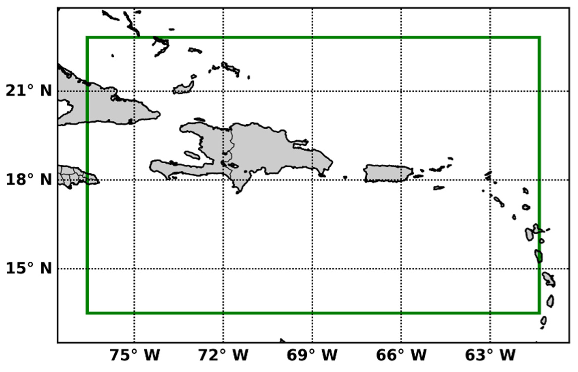
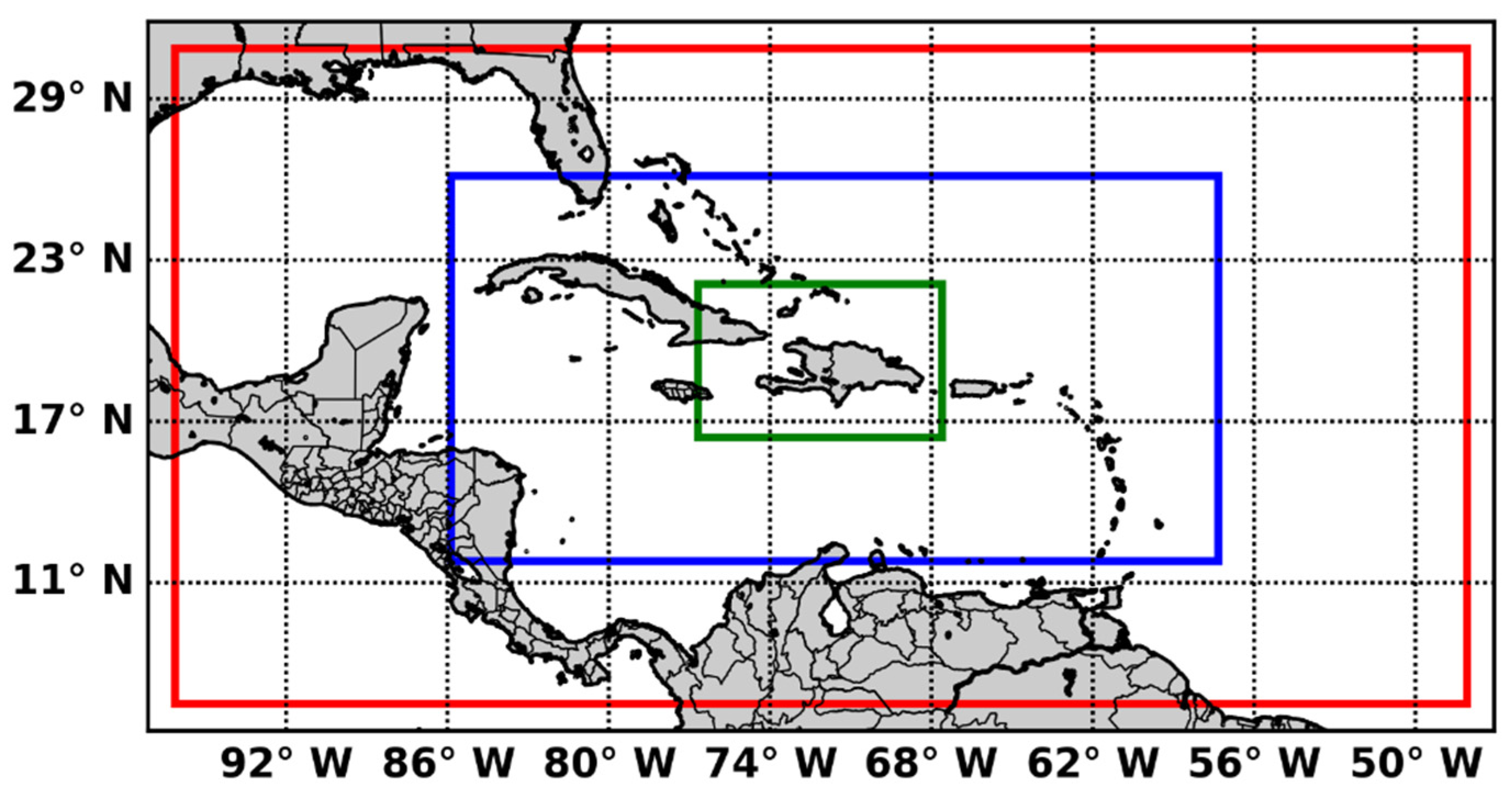
2.1. Flash Flood Guidance System

The FFGS product is developed by the Hydrologic Research Center (HRC) in San Diego (CA, USA). The primary objective of the FFGS is to provide forecasters and disaster management agencies with real-time informational guidance products related to the threat of small-scale flash floods in a specific country or region. FFGS provides products to support the development of flash flood warnings associated with rainfall events through the use of remote sensing such as radar and satellite-based rainfall estimates, numerical weather predictions and hydrological approaches.
The FFGS implemented in the Dominican Republic integrates products from the numerical forecast model Weather Research and Forecast (WRF), specifically from two dynamic cores (NonHydrostatic Mesoescale Model-NMM and Advanced Research WRF-ARW). This study evaluates the WRF products of the high-resolution window for Puerto Rico, which is elaborated by the National Center for Environmental Prediction (NCEP) (http://www.nco.ncep.noaa.gov/pmb/products/hiresw/ (accessed on 23 June 2021)). Both WRF cores (HIRESW-ARW and HIRESW-NMMB) have 5 km of spatial resolution, while the microphysics comprises WRF single-moment microphysics class 6 (WSM6 [15]) for ARW and Ferrier–Aligo for NMM [16]. These outputs are available with the 0600 and 1800 UTC initializations. Figure 1 shows the simulation domains that include the Dominican Republic.

2.2. Nowcasting and Very Short Term Forecast System

SisPI is a numerical forecasting system that also uses the WRF with the ARW core. It was developed by the Center for Atmospheric Physics of the Cuban Meteorological Institute (INSMET, in Spanish) [17,18] and implemented in the National Meteorological Office (ONAMET) of the Dominican Republic in 2019. The objective of SisPI is to provide numerical forecast precipitation to support meteorological warnings and act as a source for hydrological forecasting systems. In this case, WRF is run for three nested domains of 27, 9 and 3 km of spatial resolution with the following configurations in microphysics: WSM5 [19]; WSM5, double moment Morrison [20]; cumulus: Grell–Freitas [21]; Grell–Freitas, not activated and Planetary Boundary Layer (PBL): Mellor–Yamada–Janjic [22]; Mellor–Yamada–Janjic and Mellor–Yamada–Janjic, respectively. SisPI runs four times using the NOAA’s Global Forecast System (GFS) outputs at 0000, 0600, 1200 and 1800 UTC with 0.5 × 0.5 degrees of spatial resolution as initial and boundary conditions. Figure 2 shows the simulation domains for the Dominican Republic. The operational outputs can be consulted at http://186.149.199.244/sispi.php (accessed on 3 July 2021).

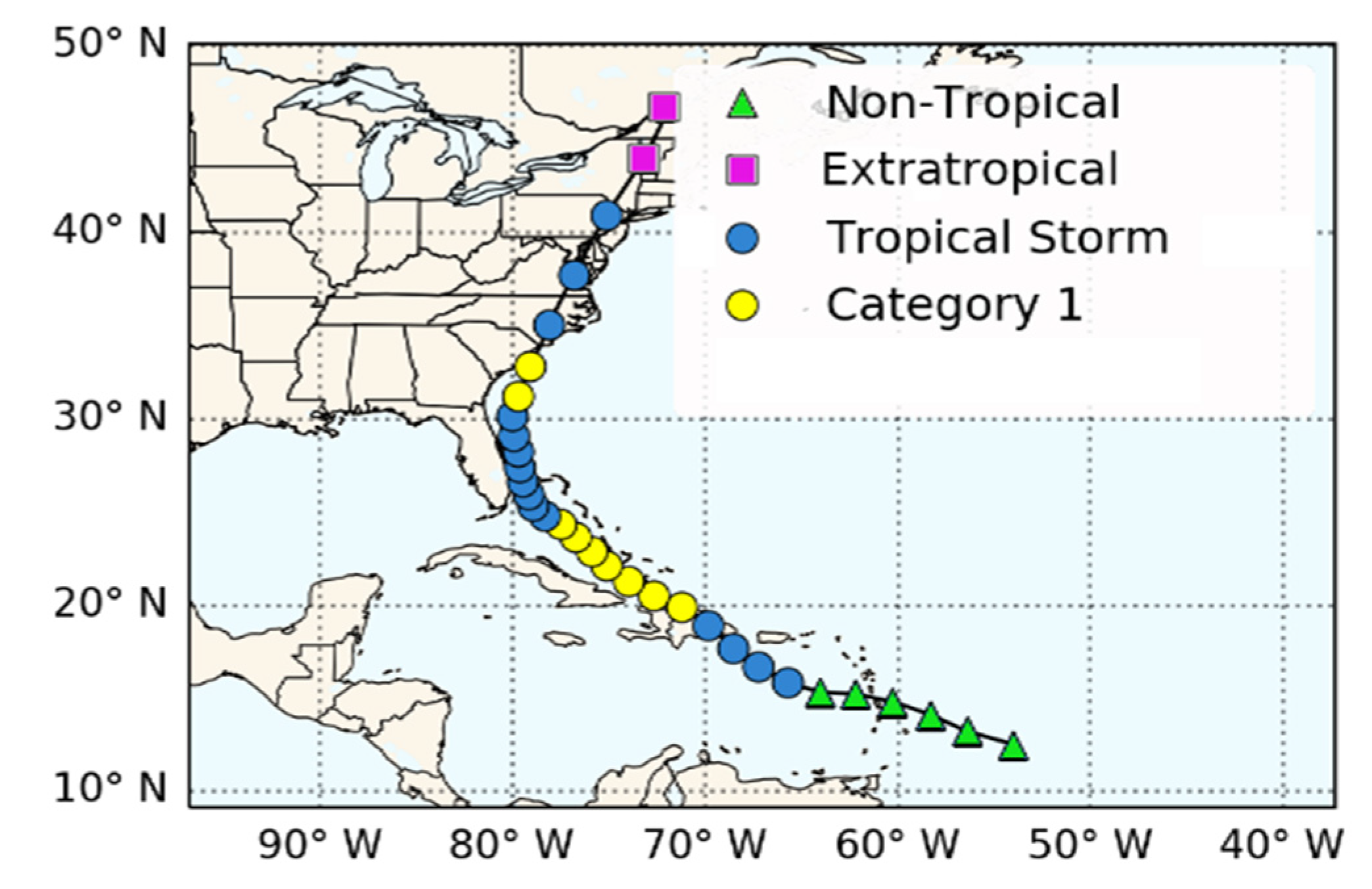
2.3. Description of Tropical Storm Isaias

Isaías was the ninth named tropical storm and the second hurricane of the 2020 cyclone season. This tropical cyclone was formed from a tropical wave that left the coasts of Africa on 23 July 2020. Several days before reaching a closed circulation and being named as a tropical cyclone by the National Hurricane Center (NHC), Isaías had already registered tropical storm force winds. Isaias impacted the Dominican Republic with its center entering through the San Pedro de Macorís province around noon on Thursday (July 30), with maximum sustained winds of up to 95 km/h and then moving northwest over the Dominican territory during the afternoon and night until it exited the national territory around midnight on Thursday. During its transit over the Dominican Republic, this tropical storm caused heavy rains accompanied by electrical storms and winds with tropical storm force (https://www.nhc.noaa.gov/data/tcr/AL092020_Isaias.pdf (accessed on 4 July 2021)). The track followed by Isaias is shown in Figure 3.
Although its center traveled through Dominican territory for about 12 h, from noon on Thursday 30 to midnight the same day, the meteorological effects began to be felt indirectly a day before and continued to affect the country a day after its passage due to the huge cloud field that accompanied this storm. The accumulated total of precipitation throughout this period of impact (both direct and indirect) translated into a maximum of 327.6 mm of rainfall recorded at the Sabana de la Mar meteorological station, followed by Samana where an accumulated 300.4 mm was recorded during 29–31 July; therefore, the east and northeast of the country were the areas that suffered the greatest rainfall impact due to the passage of this tropical storm (http://onamet.gob.do/index.php/pronosticos/temporada-ciclonica?download=4088:temporada-ciclonica-2020 (accessed on 7 July 2021)).

2.4. Data and Verification Methods

The verification was applied to the FFGS forecast products and SisPI for 30 July 2020 using, in both cases, the outputs initialized at 0600 and 1800 UTC. This process was carried out using 24 h precipitation records from 57 surface meteorological stations. These data were used to evaluate the satellite precipitation estimation generated by the GPM product in order to be used as verification references for QPFs. In particular, the Integrated Multi-satellite Retrievals for GPM (IMERG-Integrated Multi-satellite Retrievals) Final Precipitation L3 product (version 06) was used with a temporal resolution of 30 min and spatial resolution of 0.1 × 0.4 degrees [14]. For the comparison between the rain gauge and the satellite QPE, the precipitation values of the GPM product were interpolated by the nearest neighbor method to the geographic coordinates of the rain gauge data. On these interpolated values, bias and RMSE were calculated by using the verif package [23] implemented in Python. Denoting the forecast field as F and the observed field as O, the bias and RMSE are defined by the following.
b i a s = F i O i ,
R M S E = 1 N i = 1 N ( F i O i ) 2 ,
On the other hand, the verification using satellite precipitation estimation as an observation and was performed using the categorical verification method and the method for object-based diagnostic evaluation (MODE) [11,12]. Both methods require that the forecast field and the observation field be in the same grid; thus, the numerical outputs studied here were interpolated to the GPM grid using the nearest neighbor method. For the application of the first method, the numerical forecast of precipitation was considered as a dichotomous forecast by applying different thresholds [5]. The verification of this type of forecast requires the calculation of the contingency table given by the frequency of “yes” and “no” of the forecast and the observation. The combination of “yes” and “no” values between the forecast and the observation allows obtaining four categories defined as follows:
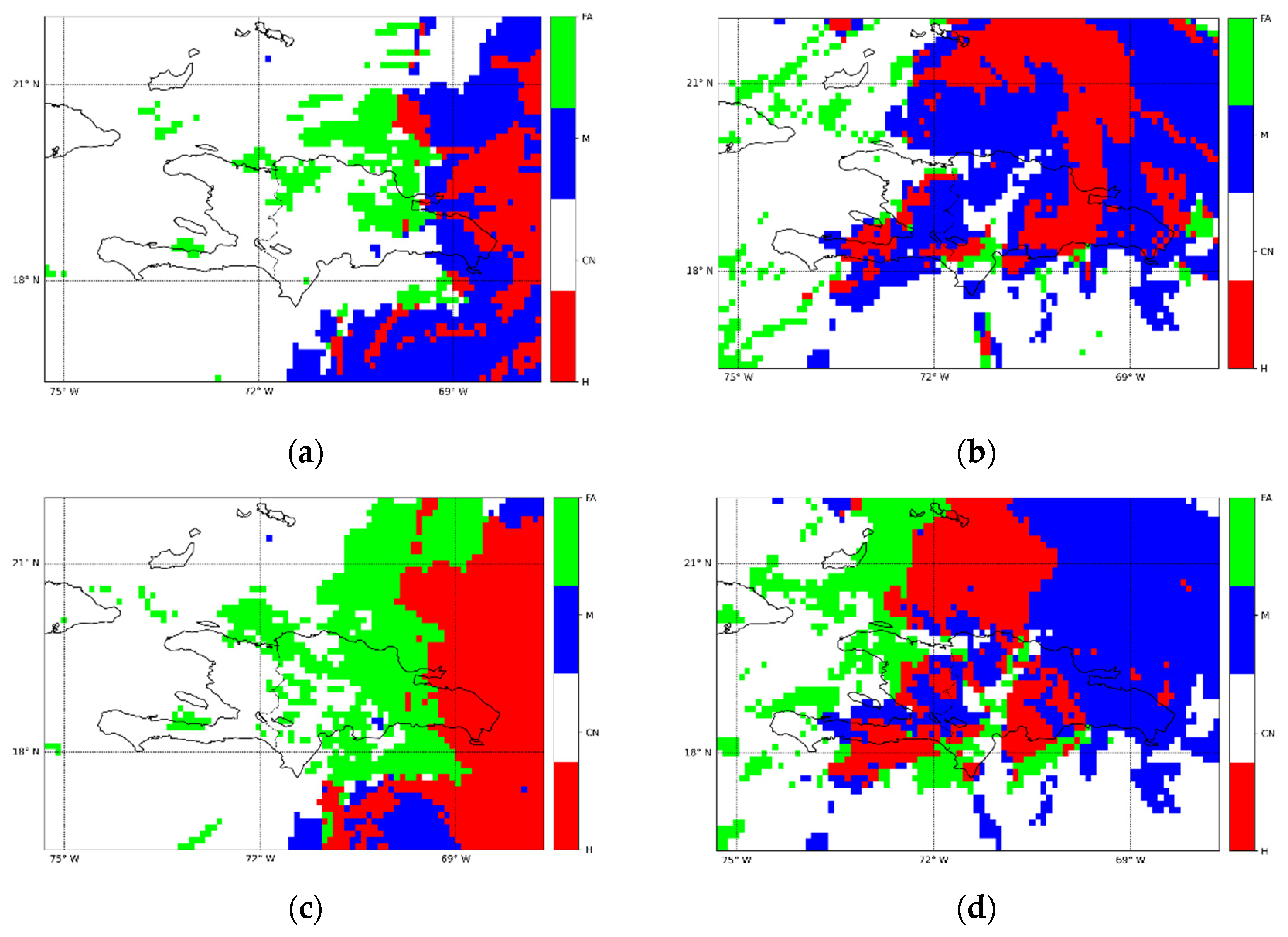
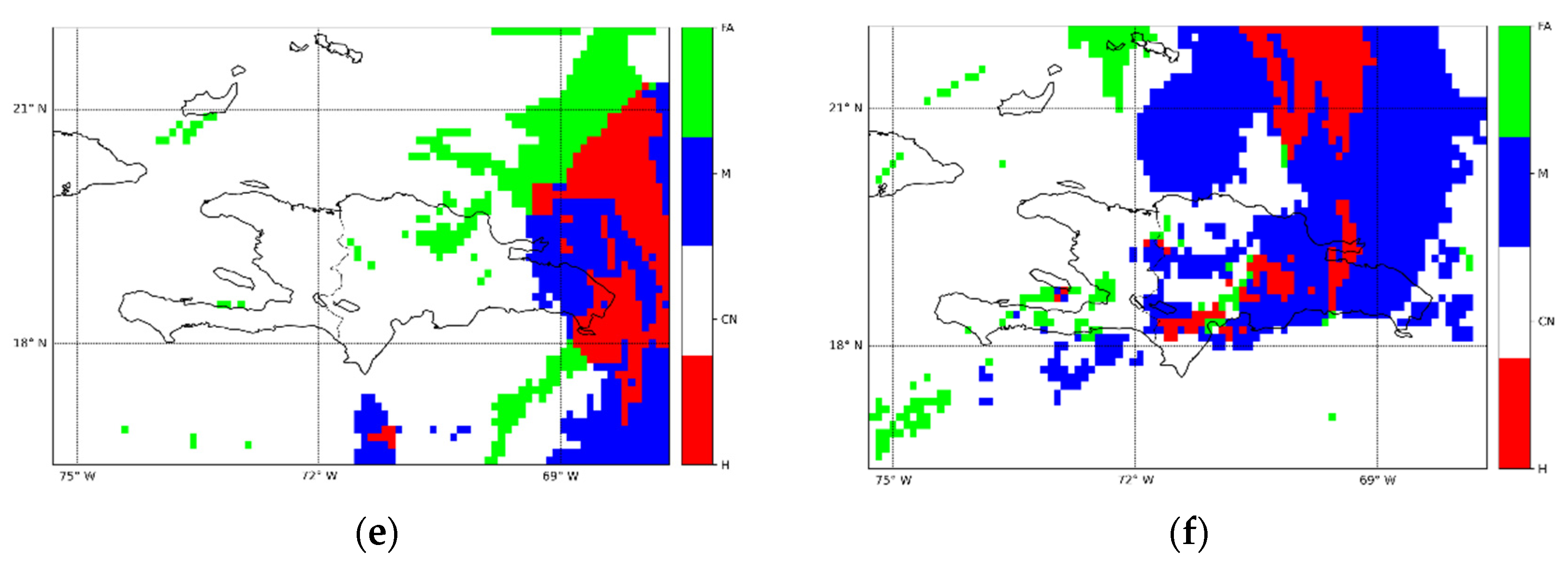
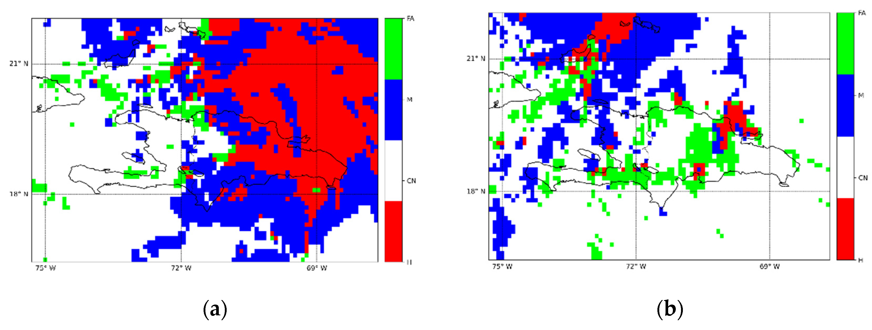
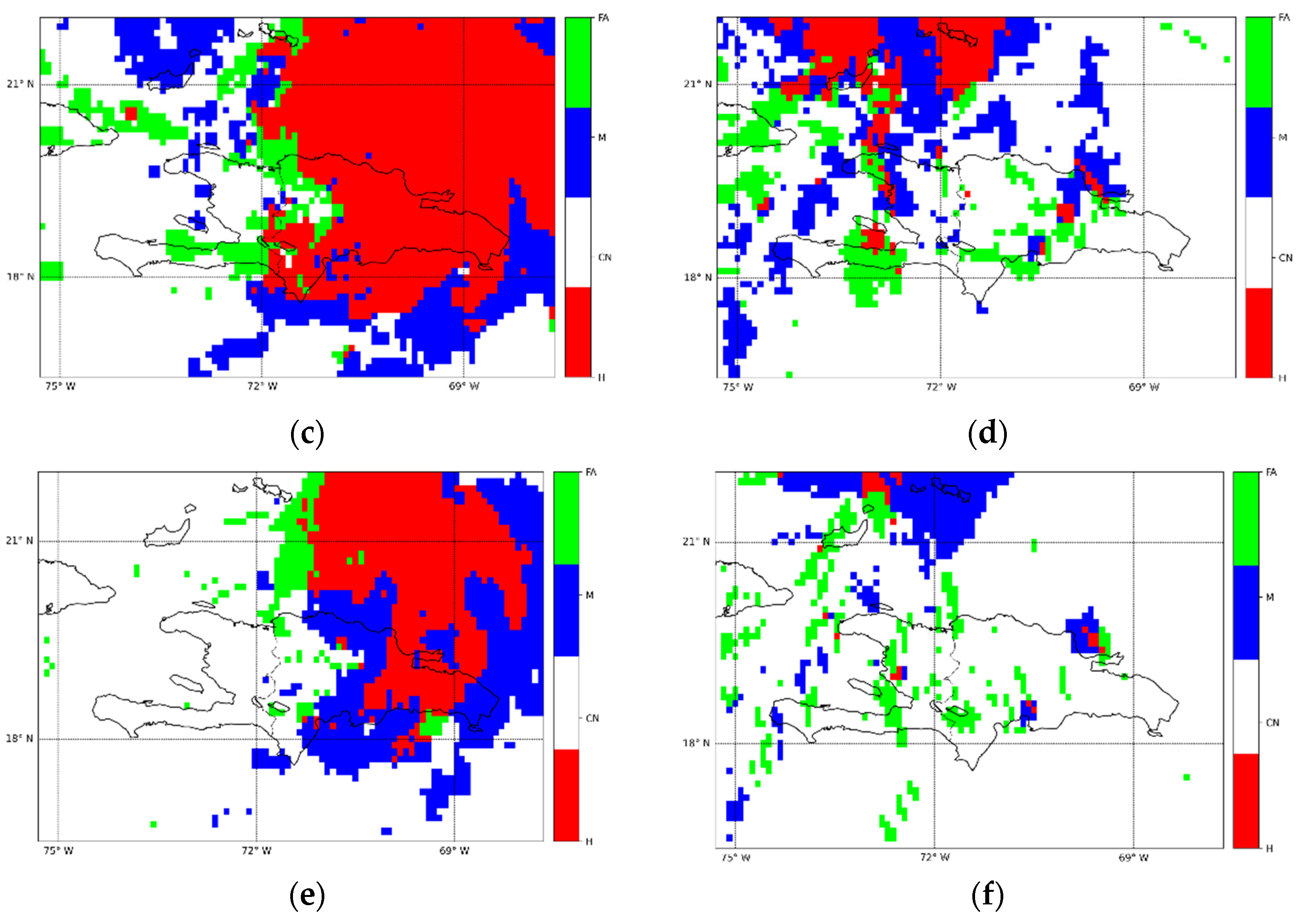
  • Hits (H): event forecast to occur and did occur;
  • Miss (M): event forecast not to occur but did occur;
  • False alarm (FA): event forecast to occur but did not occur;
  • Correct negative or correct rejection (CN): event forecast not to occur and did not occur.
From the values in the contingency table, it is possible to compute several categorical statistics. In this work, we used the Probability of Detection (POD), the Critical Success Index (CSI) and the False Alarm Rate (FAR), all given by the following expressions.
P O D = H H + M ,
F A R = F A H + F A ,
C S I = H H + M + F A .
The verification by categories was applied to know the ability of the numerical forecasting tools to predict the occurrence of the rain event using a threshold of 0.1 mm. In addition, the contingency table was calculated with thresholds of 50, 100, 150 and 200 mm to analyze the skill of the FFGS and SisPI forecast products in predicting high precipitation intensity values. Due to the fact that the numerical forecasts have high spatial resolution, the application of verification by categories is sensitive to a double penalty. The foregoing becomes evident when, due to a small error in the position of a given rain area, the error is counted twice as it is counted as a miss and also as a false alarm; therefore, it is entered twice in the calculation of the CSI, obtaining low values [5,6]. As an alternative to outcome the double penalty issue, the MODE is also applied.
The MODE is a more complex pattern recognition algorithm that consists in the application of four fundamental steps:
  • Object identification: A convolution threshold approach is used to first identify objects in forecast and observed fields. Convolution is applied for the purpose of smoothing or interpolating the original data and grouping significant areas of precipitation using a filter function as follows:
C ( x , y ) = u , v ϕ ( u , v ) f ( x u , y v ) ,
where f is the raw field, for example, the rainfall forecast from SisPI and the precipitation estimated by satellite, ϕ is the filter function and ( x , y ) and ( u , v ) are grids coordinates. Once the convoluted field C is obtained, a mask is applied from a threshold (see [24] for more details).
2.
Object properties calculation: The properties of the objects identified in both the forecast and observed field are computed. Among the main properties that are calculated, we can mention the following: the position or location of the object from the determination of the centroid, the orientation, the convex hull, the area and the perimeter.
3.
Object merging and/or matching: Using the properties of the objects, a fuzzy logic algorithm is employed for a merging or matching process depending on if the objects are from the same field or not, respectively. The fuzzy logic algorithm uses linear functions of interest to calculate the values of interest I i for each property of the objects, which are between zero (no interest) and one (maximum interest). Subsequently, confidence values C i are calculated for each property and weights ( w i ) are assigned to each one based on its relative importance. Finally, a total interest value was calculated as follows:
T ( p ) = i C i ( p ) I i ( p i ) i w i C i ( p ) ,
where p is an object property.
A threshold is applied to this total interest value (usually 0.7), and pairs of objects with T ( p ) above it are merged if they are in the same field or matched if they are in different fields [24].
4.
Verification: Is the final step and consists in computing the difference between the matched objects from the forecast and the observed field.
For a more detailed description of MODE, we recommend reviewing the following bibliography [11,12,13,25,26]. For the application of MODE in this work, the SpatialVx package from R was used [27,28]. The parameters used in the MODE are listed below:
  • Radius of the filter function in the convolution step: 3 grid points;
  • Threshold for the convolution step: 10 mm;
  • Minimum size for rain areas: 10;
  • Equal weight for the object properties;
  • Total interest threshold: 0.7.
Finally in the MODE verification step, the analysis takes into account the centroid distance, the area and the intensity errors. The latter is performed by using the lowest quartile and the 0.9 quantile.

3. Results and Discussion

A description of the results is presented below. The first section presents the comparison between precipitation measurements of rain gauge data and the precipitation estimation of GPM. Next, the results of the evaluation by categories and the evaluation applying the feature-based method are presented.

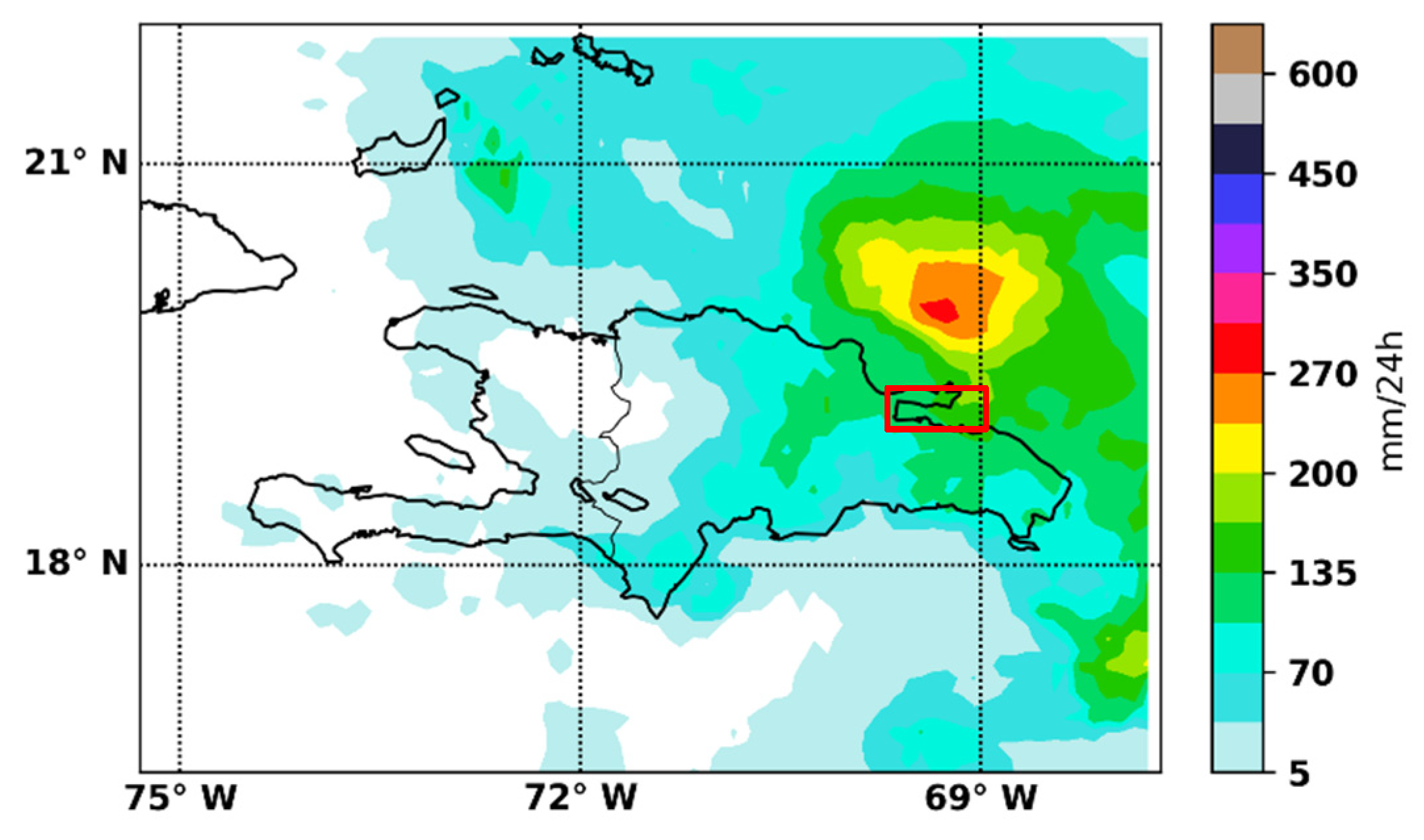
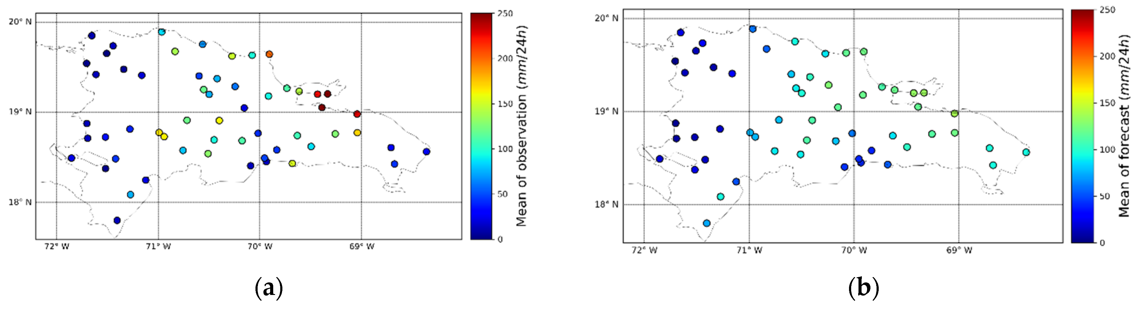
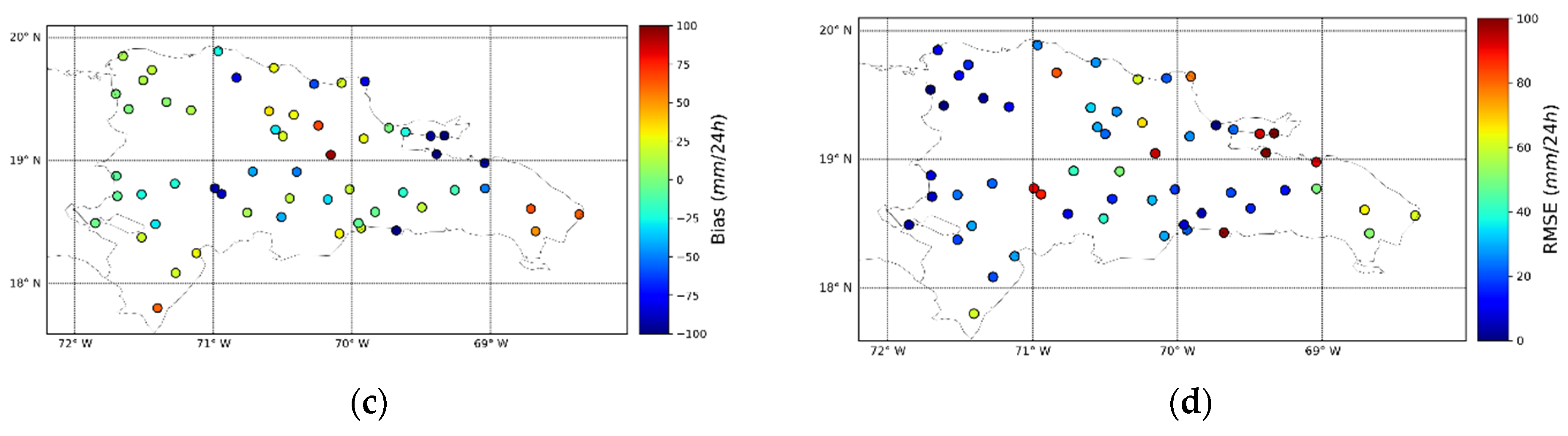
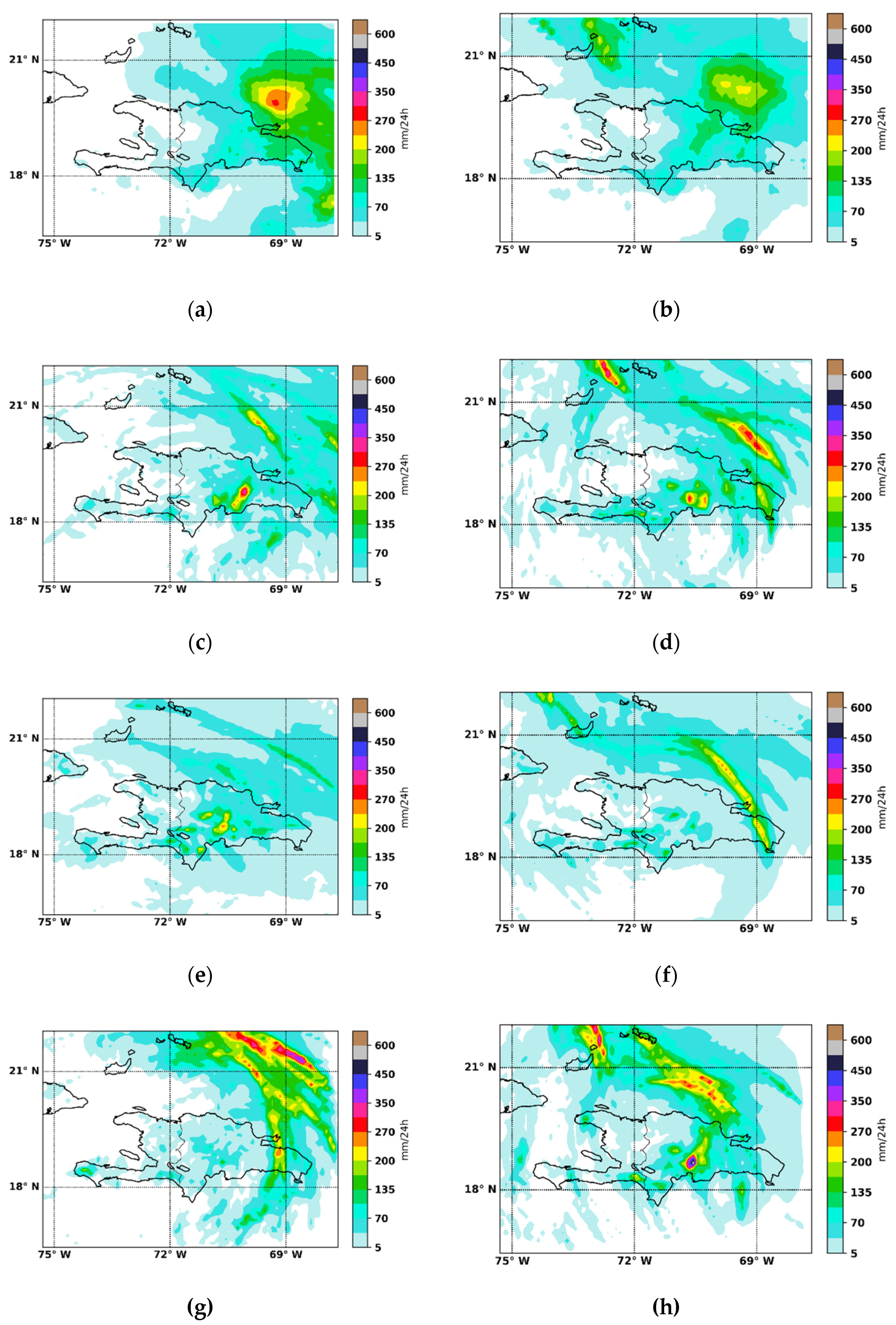
3.1. Comparison between GPM and Surface Stations

Figure 4 shows the 24 h accumulated rainfall estimated by the GPM product. The region where values of precipitation higher than 250 mm/24 h were reported is highlighted with a red square (includes Sabana del Mar 279.4 mm/24 h and Samana 276.1 mm/24 h). The precipitation estimated by GPM in the same region takes values between 100 and 200 mm/24 h, showing a clear underestimation. A more detailed analysis can be conducted by observing Figure 5, where the real values (a) and the estimated values are presented on the coordinates of the stations (b). Indeed, it is observed that an underestimation predominates over the entire Dominican territory. Figure 5c,d present the bias and RMSE values. Notice that for Sabana del Mar and Samana, a bias of −100 mm is obtained.
From another point of view, in Figure 5a,b, it can be observed that although the quantitative errors of the estimation are high, principally in those places where heavy rain occurred in terms of where precipitation was reported or not, we can say that a correspondence exists between GPM products and the data of the meteorological surface stations. Notice that GPM estimated higher values in the same places where the highest precipitations were reported and a similar behavior occurs for lower precipitation values.
Taking into account the above, it can be concluded that it is feasible to use the estimation of the precipitation of the GPM product for this case study to carry out a spatial verification in order to obtain a better coverage of the country, especially in those areas where there are no on-ground observations.

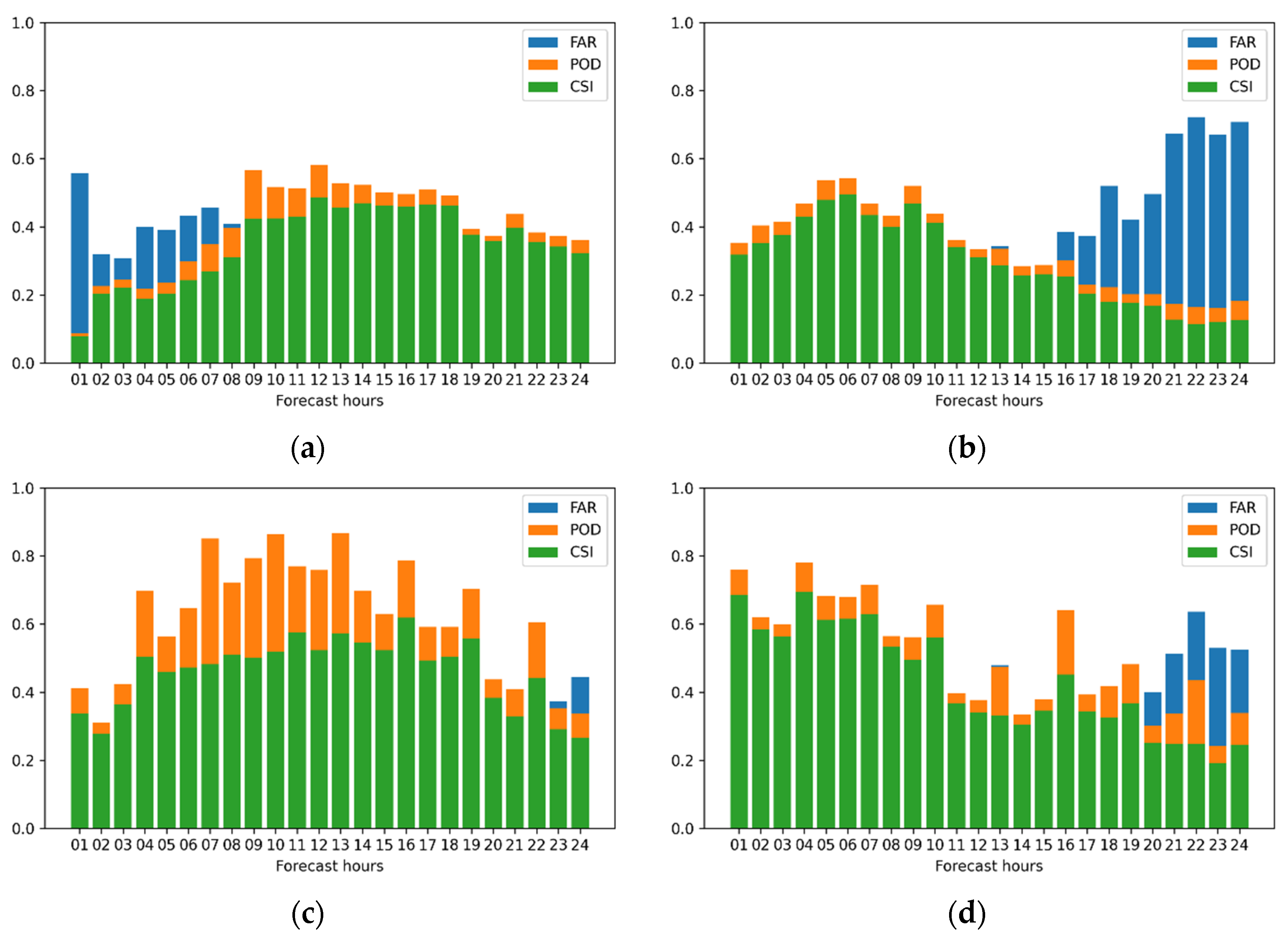
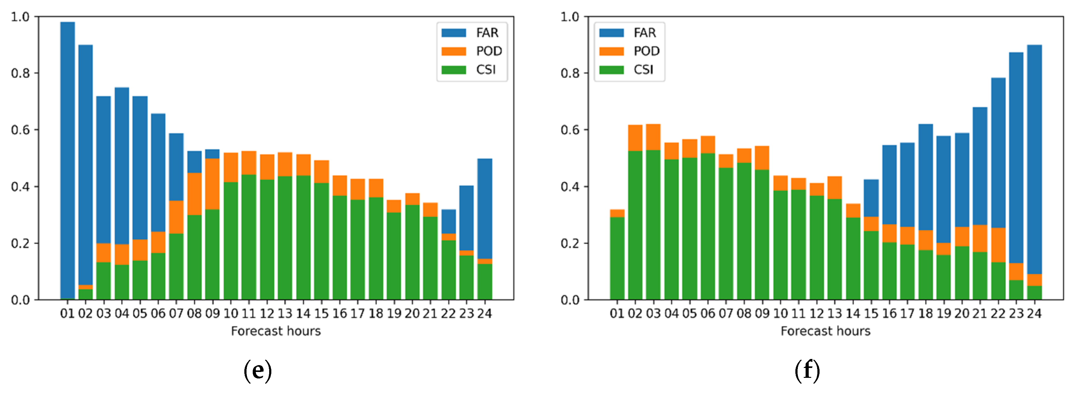
3.2. Comparison of QPFs and Satellite Estimate by Using the Categorical Verification Method

In order to know and characterize the behavior of the forecast products used by FFGS as well as the forecast generated by SisPI in the quantitative prediction of rain for 24 h, the evaluation by categories is applied for different precipitation thresholds: 0.1, 50, 100, 150 and 200 mm. With the parameters hits, misses, corrected negative and false alarms calculated, the critical success index is obtained. Table 1 shows the values of this index for each forecast and each mentioned threshold. Notice that, in the rain or no rain category (rain values higher than 0.1mm), HIRESW-NMMB presents the best performance. However, when we look at the categories that comprise extreme values, HIRESW-ARW and the SisPI have better skill, indicating that the physical configuration of these two forecast systems is more suitable to reproduce heavy rain values. For SisPI, the high spatial resolution also contributes to a better representation of these values.
A complete picture of the behavior of CSI, POD and FAR for each initialization 0600 and 1800 UTC, and each forecast step is shown in Figure 6. In this case, the contingency table and the categorical statistics were obtained by considering a threshold of 0.1 mm for rain values. Again, the forecast was obtained with HIRESW-NMMB, which reaches values of POD greater than 0.8 in various forecast periods and values greater than 0.4 for the CSI, stands out. The performance of HIRESW-NMMB for this specific weather situation suggests that this forecast tool has small errors in the position of specific rain areas. This is consistent with the fact that it is also the system that produces the fewest false alarms. On the other hand, the most discrete values are obtained with SisPI, which presents a high value relative to the false alarm index as the greatest deficiency. However, it should not be forgotten that SisPI has a higher spatial resolution than FFGS forecast products; thus, the number of false alarms may be affected because misses are also counted as false alarms. Therefore, the CSI values are much more discrete for SisPI.
Figure 7 and Figure 8 allow an approach to the behavior of the evaluation metrics from the spatial point of view considering the rain/no rain event (a threshold of 0.1 mm). Figure 7 shows the spatial distribution of hits, misses, corrected negative and false alarms for the forecast for 30 July 2020 1400 UTC and 31 July 2020 0500 UTC, generated by the three forecast systems with initializations at 0600 UTC. It is evident that the highest number of hits is exhibited by HIRESW-NMMB at the same time that HIRESW-ARW and SisPI show higher areas of misses and false alarms.
In Figure 8, the same metrics are shown but only for runs initialized at 1800 UTC and the forecast periods. An increase in the hit areas is observed, with HIRESW-NMMB still being the system with the best results. Notice that the results presented in Figure 7 and Figure 8 highlight that the point-matching categorical methodology, although it is intuitive and very easy to understand, is more strict regarding when a forecast is correct or not. This may, in situations such as the one shown in Figure 7e,f and Figure 8e,f, suggest that the forecast had very low skill to predict rain bands associated with tropical storm Isaías. However, it can be observed that the values of false alarms and misses are mostly associated with a displacement of the referred rain areas. In other words, it can be noted that the forecasts manage to represent the shape of the rain areas, failing to locate them and not in predicting the occurrence of the event. This displacement error presented fundamentally by SisPI is, among other factors, the reason why the skill of SisPI is so low and reveals the sensitivity of the verification method to the double penalty problem. In order to overcome this issue, the evaluation with the approach based on the characteristics and shape of the rain areas is presented below.

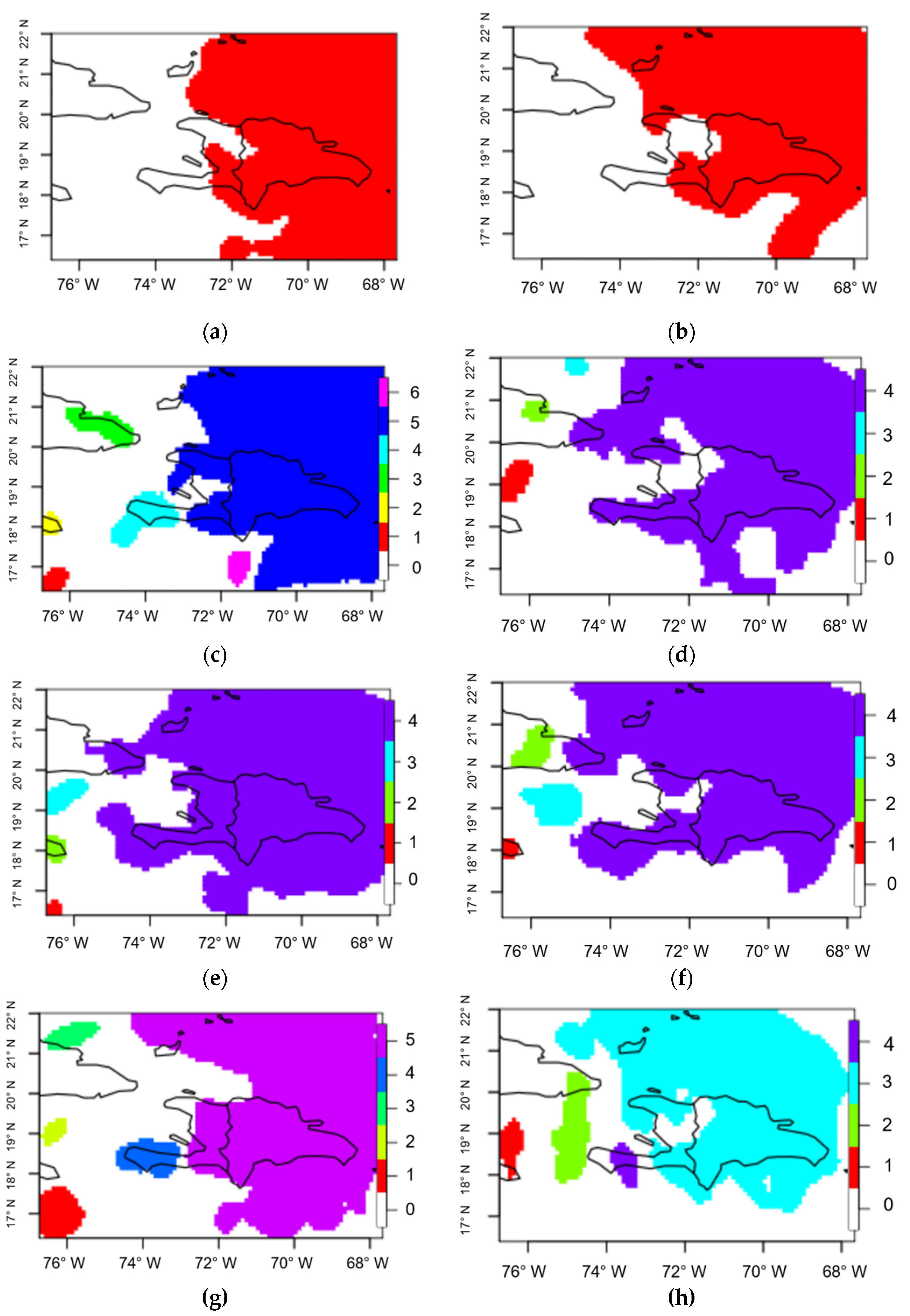
3.3. Application of the Feature-Based Verification Approach

For the verification using an object-oriented approach, the 24 h accumulated precipitations predicted by each forecasting tool under evaluation were taken. Figure 9 shows these accumulated for the experiments initialized at 0600 UTC and 1800 UTC. The results of applying the MODE method are presented in Figure 10. Note that only one object is identified in the observation, Figure 10a,b, while in the forecasts (HIRESW-ARW Figure 10c,d; HIRESW-NMMB Figure 10e,f; and SisPI Figure 10g,h), the number of objects oscillates between four and six, indicating the occurrence of false alarms, which is consistent with the verification method previously applied. Nevertheless, as in this variant of numerical forecast verification, the grid points are grouped into objects and the objects are discarded (if have an area less than 10) and merged (if are very near); the final number of identified objects is greater than in observation, although it represents a lower number of false alarms.
Table 2 shows some features statistics obtained for the objects that were associated or matched by the MODE approach. Observe that the forecast field objects associated with the unique object identified in the observation for the 0600 UTC run are those labeled with numbers 5, 4 and 5 for HIRESW-ARW, HIRESW-NMMB and SisPI, respectively; while for the 1800 UTC run, the objects are identified by labels 4, 4 and 3. In this analysis, as we mentioned before, we will be reviewing, in particular, the distance between the centroids, the area, the intensity errors determined using the the lower quartile and the 0.9 quantile of precipitation amount within objects and the total interest. The high values of the total interest among the associated objects suggest that they have similar morphological characteristics and similar precipitation amounts. The distance between the centroids and the area of the features is a sample of the similarities presented. Note how the HIRESW-NMMB product had the lowest values of total interest, which may be related to the errors in the position of the object since it presents the greatest distances between the centroids. In addition, it is also observed that this forecast product of the FFGS overestimated the area occupied by the object, which translates into a spatial overestimation of precipitation.
The 0.25 quartile threshold for the HIRESW-NMMB is 10.6 and 16.6 mm for the runs initialized at 0600 and 1800 UTC, respectively, which are very close to the thresholds obtained with satellite-based QPE (21.7 and 28.8 mm). HIRESW-ARW and SisPI had a similar behavior for these precipitation values. The largest differences in the skill of the forecasting tools were observed in the 0.9 quantile. The HIRESW-NMMB predicted values well below what was observed. For the 0600 UTC run, the threshold obtained in the observed field is 146.9 mm, and in the HIRESW-ARW, HIRESW-NMMB and SisPI forecast fields, the thresholds were 91.0, 68.7 and 166.0 mm, respectively. This behavior indicates an underestimation of precipitation intensity in the forecasts of FFGS products, which is more evident in the HIRESW-NMMB product. SisPI, however, presented a slight overestimation. Regarding the amount and intensity of precipitation, it can be concluded that HIRESW-NMMB presented less skill for this case study fundamentally in the forecast of heavy rain. This is consistent with results presented in Table 1 obtained from the application of the categorical verification method using different precipitation thresholds. SisPI and HIRESW-ARW stand out as having the best ability to predict high precipitation values in the experiments initialized at 0600 UTC and 1800 UTC, respectively.

4. Conclusions

The work presented constitutes an extension of the evaluation of the quantitative precipitation forecast of FFGS and SisPI systems for the case of Tropical Storm Isaías, which affected the Dominican Republic in July 2020. The assessment was carried out on forecasts for 30 July 2020, with initialization at 0600 and 1800 UTC and taking the satellite estimation of the GPM product as the reference precipitation. According to the results obtained previously with the use of a verification method by categories, both tools had good performance for the forecast of precipitation, with the HIRESW-NMMB product of the FFGS being the one with the best indicators for the forecast of the occurrence of precipitation and for moderate values of this field. The HIRESW-ARW and SisPI products were better for the forecast of heavy rain. However, both products also presented high values of the false alarm rate, with SisPI being the one with the worst behavior. In this extension, the study of these tools was continued with the aim of delving into the results obtained and answering some questions that remained pending, for example, are the low CSI values presented by SisPI product of an error in the position of the precipitation areas or due to misses in the forecast of the precipitation occurrence? Are high FAR values related to an incorrect physical representation of the meteorological event or are they also linked to position errors? For this case study, why does the high spatial resolution SisPI not have added value? Could it be the case that the problem of the double penalty that may occur in the evaluation by categories of high spatial resolution forecasts may be affecting the indicators obtained for SisPI? To address these questions, a spatial verification approach was applied using MODE, a method that is not sensitive to the double penalty problem when evaluating forecasts at high spatial resolution. The main conclusions reached with the investigation are listed below:
  • The evaluation of the accumulated rainfall in 24 h and using different precipitation thresholds indicates that the three tools had good skill to forecast low precipitation values with CSI values greater than 0.6, being slightly better the HIRESW-NMMB product with CSI values of 0.8. A similar result was obtained with the spatial evaluation using MODE, where it is shown that the three modeling tools presented differences that did not exceed 15 mm in the 0.25 quartile. The evaluation by categories also shows that HIRESW-ARW and SisPI had a better behavior for the forecast of intense precipitation, although the values less than 0.1 of the CSI indicate poor skill. However, the results obtained with the MODE do highlight the good skill of the HIRESW-ARW and SisPI, since in the 0.9 quantile, the differences did not exceed 30 mm in both runs, while in the prediction of the HIRESW-NMMB, the differences were greater than 60 mm.
  • The difference between the number of objects identified in the forecast fields (between four and five in all runs) and in the observation (one single object) indicates the existence of false alarms. However, when compared to the behavior of FAR calculated with the evaluation by categories, both HIRESW-ARW and the SisPI exhibit a behavior similar to HIRESW-NMMB, showing that the high values of FAR obtained in the previous result are linked to position errors that are larger and more frequent in the case of SisPI as it has higher spatial resolution.
  • The evaluation by categories suggests, based on the spatial distribution of hits, errors, false alarms and corrected negatives, that the low CSI values presented by the SisPI modeling tool are mainly due to an error in the predicted position of the areas of rain and not to an error in the forecast of the occurrence of rain. In this sense, the spatial verification approach clearly reveals these position errors since it identifies and associates precipitation areas with similar characteristics in terms of area and rainfall intensity but with a slight difference in the centroids.
  • Despite the differences presented, in general, HIRESW-NMMB, HIRESW-ARW and SisPI presented good ability to forecast the precipitation areas associated with Isaías. Unlike the previous result, by applying a spatial verification method that is not sensitive to double penalty and that includes information about the shape of the rain areas, the position and the intensity, the result is obtained where HIRESW-ARW and SisPI present slightly higher total interest values, which indicates them as tools with better performances. In particular, SisPI, for this case study, turned out to be more appropriate for the forecast of intense precipitation values, which may be linked, among other aspects, to the increase in spatial resolution.
As a continuation of the work, applying verification methods to other meteorological situations is suggested, such as mesoscale convective systems and orographic rain. In addition, in the MODE, using higher thresholds that allow isolating and highlighting the areas of heavy rain is recommended in order to characterize the skill of the forecast tools to properly locate them. On the other hand, it is also recommended to use, as observation for the accumulated data in 24 h, a merged grid from GPM data and rain gauge data.

Author Contributions

Conceptualization, M.S.-L. and J.M.; methodology, M.S.-L., J.M. and A.F.-B.; software, M.S.-L., S.A.-Á. and A.F.-B.; validation, M.S.-L., S.A.-Á., A.F.-B. and M.S.-L.; formal analysis, J.M. and M.S.-L.; investigation, M.S.-L.; resources, J.M. and M.S.-L.; data curation, M.S.-L. and A.F.-B.; writing—original draft preparation, M.S.-L. and T.G.; writing—review and editing, M.S.-L., J.M., J.S. and T.G.; visualization, M.S.-L. and A.F.-B.; supervision, M.S.-L. and T.G. All authors have read and agreed to the published version of the manuscript.

Funding

This research has been undertaken as part of the project “Building Resilience to High-Impact Hydro-meteorological Events through Strengthening Multi-Hazard Early Warning Systems (MHEWS) in Small Island Developing States (SIDS) and Southeast Asia (SEA)” and the APC was funded by WMO.

Institutional Review Board Statement

Not applicable.

Informed Consent Statement

Not applicable.

Data Availability Statement

The data from the numerical forecasting systems evaluated in this investigation are available at http://186.149.199.244/data/ (accessed on 4 July 2021).

Acknowledgments

The authors wants to thanks the support provided under the Caribbean component of the Canada CREWS project: “Building Resilience to High-Impact Hydro-meteorological Events through Strengthening Multi-Hazard Early Warning Systems (MHEWS) in Small Island Developing States (SIDS) and Southeast Asia (SEA)”, funded by the Environment and Climate Change of Canada (ECCC). https://community.wmo.int/activity-areas/hydrology-and-water-resources/IRFF-in-Dominican-Republic (accessed on 26 October 2021).

Conflicts of Interest

The authors declare no conflict of interest.

References

  1. Erickson, M.J.; Kastman, J.S.; Albright, B.; Perfater, S.; Nelson, J.A.; Schumacher, R.S.; Herman, G.R. Verification Results from the 2017 HMT–WPC Flash Flood and Intense Rainfall Experiment. J. Appl. Meteorol. Climatol. 2019, 58, 2591–2604. [Google Scholar] [CrossRef]
  2. Aksoy, M. Evaluation of Numerical Weather Prediction Models for Flash Flood Warnings in Turkey. Master’s Thesis, Middle East Technical University, Çankaya/Ankara, Turkey, 2020. [Google Scholar]
  3. Sierra-Lorenzo, M.; Bezanilla-Morlot, A.; Centella-Artola, A.D.; León-Marcos, A.; Borrajero-Montejo, I.; Ferrer-Hernández, A.L.; Salazar-Gaitán, J.L.; Lau-Melo, A.; Picado-Traña, F.; Pérez-Fernández, J. Assessment of Different WRF Configurations Performance for a Rain Event over Panama. Atmos. Clim. Sci. 2020, 10, 280. [Google Scholar] [CrossRef]
  4. Zawadzki, I.I. Statistical Properties of Precipitation Patterns. J. Appl. Meteorol. Climatol. 1973, 12, 459–472. [Google Scholar] [CrossRef]
  5. Rossa, A.; Nurmi, P.; Ebert, E. Overview of Methods for the Verification of Quantitative Precipitation Forecasts. In Precipitation: Advances in Measurement, Estimation and Prediction; Springer: Berlin/Heidelberg, Germany, 2008; pp. 419–452. [Google Scholar]
  6. Ebert, E. WWRP/WGNE Joint Working Group on Verification. Forecast Verification–Issues, Methods and FAQ. 2005. Available online: http://www.cawcr.gov.au/projects/verification/ (accessed on 26 October 2021).
  7. Ebert, E.E.; Janowiak, J.E.; Kidd, C. Comparison of Near-Real-Time Precipitation Estimates from Satellite Observations and Numerical Models. Bull. Am. Meteorol. Soc. 2007, 88, 47–64. [Google Scholar] [CrossRef] [Green Version]
  8. Ebert, E.E. Fuzzy Verification of High-Resolution Gridded Forecasts: A Review and Proposed Framework. Meteorol. Appl. J. Forecast Pract. Appl. Train. Tech. Model. 2008, 15, 51–64. [Google Scholar] [CrossRef]
  9. Casati, B.; Ross, G.; Stephenson, D.B. A New Intensity-Scale Approach for the Verification of Spatial Precipitation Forecasts. Meteorol. Appl. 2004, 11, 141–154. [Google Scholar] [CrossRef] [Green Version]
  10. Ebert, E.E.; McBride, J.L. Verification of Precipitation in Weather Systems: Determination of Systematic Errors. J. Hydrol. 2000, 239, 179–202. [Google Scholar] [CrossRef]
  11. Davis, C.; Brown, B.; Bullock, R. Object-Based Verification of Precipitation Forecasts. Part I: Methodology and Application to Mesoscale Rain Areas. Mon. Weather Rev. 2006, 134, 1772–1784. [Google Scholar] [CrossRef] [Green Version]
  12. Davis, C.; Brown, B.; Bullock, R. Object-Based Verification of Precipitation Forecasts. Part II: Application to Convective Rain Systems. Mon. Weather Rev. 2006, 134, 1785–1795. [Google Scholar] [CrossRef] [Green Version]
  13. Davis, C.A.; Brown, B.G.; Bullock, R.; Halley-Gotway, J. The Method for Object-Based Diagnostic Evaluation (MODE) Applied to Numerical Forecasts from the 2005 NSSL/SPC Spring Program. Weather Forecast 2009, 24, 1252–1267. [Google Scholar] [CrossRef] [Green Version]
  14. Hou, A.Y.; Kakar, R.K.; Neeck, S.; Azarbarzin, A.A.; Kummerow, C.D.; Kojima, M.; Oki, R.; Nakamura, K.; Iguchi, T. The Global Precipitation Measurement Mission. Bull. Am. Meteorol. Soc. 2014, 95, 701–722. [Google Scholar] [CrossRef]
  15. HONG, S.-Y. The WRF Single-Moment 6-Class Microphysics Scheme (WSM6). J. Korean Meteor. Soc. 2006, 42, 129–151. [Google Scholar]
  16. Aligo, E. The New-Ferrier-Aligo Microphysics in the NCEP 3-Km NAM Nest. In Proceedings of the 97th AMS Annual Meeting, Seattle, WA, USA, 22–26 January 2017; pp. 21–26. [Google Scholar]
  17. Sierra-Lorenzo, M.; Ferrer-Hernández, A.L.; Valdés-Hernández, R.; González-Mayor, Y.; Cruz-Rodríguez, R.C.; Borrajero-Montejo, I.; Rodríguez-Genó, C.F.; Quintana-Rodríguez, N.; Roque-Carrasco, A. Sistema Automático de Predicción Mesoescala de Cuatro Ciclos Diarios; Informe de Resultado, Instituto de Meteorología: La Habana, Cuba, 2015. [Google Scholar] [CrossRef]
  18. Sierra-Lorenzo, M.; Borrajero-Montejo, I.; Ferrer-Hernández, A.L.; Morfá-Ávalos, Y.; Morejón-Loyola, Y.; Hinojosa-Fernández, M. Estudios de Sensibilidad Del SisPI a Cambios de La PBL, La Cantidad de Niveles Verticales y, Las Parametrizaciones de Microfísica y Cúmulos, a Muy Alta Resolución; Informe de Resultado, Instituto de Meteorología: La Habana, Cuba, 2017. [Google Scholar] [CrossRef]
  19. Lim, J.-O.J.; Hong, S.; Dudhia, J. The WRF Single-Moment-Microphysics Scheme and Its Evaluation of the Simulation of Mesoscale Convective Systems. In Proceedings of the 20th Conference on Weather Analysis and Forecasting/16th Conference on Numerical Weather Prediction, Seattle, WA, USA, 10 January 2004. [Google Scholar]
  20. Morrison, H.; Curry, J.A.; Khvorostyanov, V.I. A New Double-Moment Microphysics Parameterization for Application in Cloud and Climate Models. Part I: Description. J. Atmos. Sci. 2005, 62, 1665–1677. [Google Scholar] [CrossRef]
  21. Grell, G.A.; Freitas, S.R. A Scale and Aerosol Aware Stochastic Convective Parameterization for Weather and Air Quality Modeling. Atmos. Chem. Phys. 2014, 14, 5233–5250. [Google Scholar] [CrossRef] [Green Version]
  22. Janjić, Z.I. The Step-Mountain Eta Coordinate Model: Further Developments of the Convection, Viscous Sublayer, and Turbulence Closure Schemes. Mon. Weather Rev. 1994, 122, 927–945. [Google Scholar] [CrossRef] [Green Version]
  23. Nipen, T. Verif: A Verification Program for Meteorological Forecasts and Observations. Available online: https://github.com/WFRT/verif/wiki/ (accessed on 26 October 2021).
  24. Jensen, T.; Brown, B.; Bullock, R.; Fowler, T.; Gotway, J.H.; Newman, K. Model Evaluation Tools Version 9.0. 2 User’s Guide; Developmental Testbed Center: Boulder, CO, USA, 2020. [Google Scholar]
  25. Rodríguez Genó, C.F.; Sierra Lorenzo, M.; Ferrer Hernández, A.L. Modificación e Implementación Del Método de Evaluación Espacial MODEMod Para Su Uso Operativo En Cuba. Cienc. Tierra El Espac. 2016, 17, 18–31. [Google Scholar]
  26. Carrasco, A.R.; Sapucci, L.F.; Mattos, J.G.Z.d.; Lorenzo, M.S.; Montejo, I.B. Explorando as Particularidades Do Método Orientado a Objetos Na Avaliação Das Previsões de Precipitação. Rev. Bras. Meteorol. 2020, 35, 317–333. [Google Scholar] [CrossRef]
  27. Gilleland, E. Comparing Spatial Fields with SpatialVx: Spatial Forecast Verification in R. J. Stat. Softw. 2021, 55, 69. [Google Scholar]
  28. Gilleland, E. SpatialVx: Spatial Forecast Verification; Developmental Testbed Center: Boulder, CO, USA, 2021. [Google Scholar]
Figure 1. The green square represents the simulation domain for HIRESW-ARW and HIRESW-NMMB that includes Dominican Republic.
Atmosphere 13 00495 g001
Figure 2. Simulation domains for SisPI. The red, blue and green squares represent the areas with resolutions of 27, 9 and 3 km, respectively.
Atmosphere 13 00495 g002
Figure 3. Hurricane Isaias’ track.
Atmosphere 13 00495 g003
Figure 4. Precipitation estimated for 24 h by the GPM product for 30 July 2020. The red rectangle highlights the areas where the highest accumulated values were registered.
Atmosphere 13 00495 g004
Figure 5. Precipitation measurements reported by surface stations (a) and precipitation estimated by the GPM product interpolated at the stations coordinates (b). The bias and RMSE metrics are shown in panels (c) and (d), respectively.
Atmosphere 13 00495 g005aAtmosphere 13 00495 g005b
Figure 6. CSI, POD and FAR index for 0600 (a,c,e) and 1800 (b,d,f) runs for 30 July 2020 of HIRESW-ARW (a,b), HIRESW-NMMB (c,d) and SisPI (e,f).
Atmosphere 13 00495 g006aAtmosphere 13 00495 g006b
Figure 7. Hits, misses, corrected negative and false alarms (0.1 threshold) for 30 July 2020 runs initialized at 0600 UTC: 30 July, at 1400 UTC forecast time (a,c,e), and 31 July, at 0500 UTC forecast time (b,d,f). Results for HIRESW-ARW, HIRESW-NMMB and SisPI are shown in panels (a,b), (c,d) and (e,f) respectively.
Atmosphere 13 00495 g007aAtmosphere 13 00495 g007b
Figure 8. Hits, misses, corrected negative and false alarms (0.1 threshold) for the 30 July 2020 runs initialized at 1800 UTC: at 31 July, at 0100 UTC forecast time (a,c,e), and 31 July, at 1800 UTC forecast time (b,d,f). Results for HIRESW-ARW, HIRESW-NMMB and SisPI are shown in the panels (a,b), (c,d) and (e,f) respectively.
Atmosphere 13 00495 g008aAtmosphere 13 00495 g008b
Figure 9. Observed and forecast accumulated precipitation in 24 h started from 0600 UTC of 30 July 2020 to 0600 UTC of 31 July 2020 (a,c,e,g) and started from 1800 UTC of 30 July 2020 to 1800 UTC of 31 July 2020 (b,d,f,h). GPM precipitation estimation is presented in panels (a,b), while the forecast rainfall for HIRESW-ARW, HIRESW-NMMB and SisPI are shown in panels (a,b), (c,d) and (e,f), respectively.
Atmosphere 13 00495 g009
Figure 10. Observed and forecast features or objects detected from 0600 UTC of 30 July 2020 to 0600 UTC of 31 July 2020 (a,c,e,g) and from 1800 UTC of 30 July 2020 to 1800 UTC of 31 July 2020 (b,d,f,h). GPM features are presented in panels (a,b) while the forecast features for HIRESW-ARW, HIRESW-NMMB and SisPI are show in the panels (a,b), (c,d) and (e,f), respectively.
Atmosphere 13 00495 g010
Table 1. CSI values for the 24 h rainfall forecast of the HIRESW-ARW, HIRESW-NMMB and SisPI.
Threshold (mm/h)HIRESW-ARW
0600/1800
HIRESW-NMMB
0600/1800
SisPI
0600/1800
0.10.7250.8510.8240.8520.6680.702
500.4570.4840.2630.2690.3970.472
1000.1380.2740.0420.1360.3170.254
1500.0380.1600.0030.1320.1770.129
2000.0250.10.00.0480.0410.009
Table 2. Attributes values for features identified in the 24 h rainfall forecast of HIRESW-ARW, HIRESW-NMMB and SisPI.
GPM Feature
0600/1800
HIRESW-ARW
0600/1800
HIRESW-NMMB
0600/1800
SisPI
0600/1800
1544453
Total Interest0.900.910.890.880.900.92
Centroid Distance0.440.420.890.930.370.81
Area
25842494250125873139267426002284
Intensity0.25
21.728.813.01910.616.611.916.3
Intensity0.9
146.9123.391.0112.068.781.4166.1145.5
Publisher’s Note: MDPI stays neutral with regard to jurisdictional claims in published maps and institutional affiliations.

