
Simulation and Evaluation of Statistical Downscaling of Regional Daily Precipitation over North China Based on Self-Organizing Maps


1
School of Remote Sensing and Geomatics Engineering, Nanjing University of Information Science and Technology, Nanjing 210044, China
2
Key Laboratory of Meteorological Disaster, Ministry of Education (KLME), Joint International Research Laboratory of Climate and Environment Change (ILCEC), Collaborative Innovation Center on Forecast and Evaluation of Meteorological Disasters (CIC-FEMD), Jiangsu Key Laboratory of Meteorological Observation and Information Processing, Jiangsu Technology & Engineering Center of Meteorological Sensor Network, School of Electronic & Information Engineering, Nanjing University of Information Science and Technology, Nanjing 210044, China
*
Author to whom correspondence should be addressed.
Atmosphere 2022, 13(1), 86; https://doi.org/10.3390/atmos13010086
Submission received: 29 November 2021
/
Revised: 29 December 2021
/
Accepted: 4 January 2022
/
Published: 6 January 2022
(This article belongs to the Special Issue Climate Variability and Climate Extreme Events over Asia on Various Time-Scales since the Last Glacial Maximum)
Abstract
:A statistical downscaling method based on Self-Organizing Maps (SOM), of which the SOM Precipitation Statistical Downscaling Method (SOM-SD) is named, has received increasing attention. Herein, its applicability of downscaling daily precipitation over North China is evaluated. Six indices (total season precipitation, daily precipitation intensity, mean number of precipitation days, percentage of rainfall from events beyond the 95th percentile value of overall precipitation, maximum consecutive wet days, and maximum consecutive dry days) are selected, which represent the statistics of daily precipitation with regards to both precipitation amount and frequency, as well as extreme event. The large-scale predictors were extracted from the National Center for Environmental Prediction/National Center for Atmospheric Research (NCEP/NCAR) daily reanalysis data, while the prediction was the high resolution gridded daily observed precipitation. The results show that the method can establish certain conditional transformation relationships between large-scale atmospheric circulation and local-scale surface precipitation in a relatively simple way. This method exhibited a high skill in reproducing the climatologic statistical properties of the observed precipitation. The simulated daily precipitation probability distribution characteristics can be well matched with the observations. The values of Brier scores are between 0 and 1.5 × 10⁻⁴ and the significance scores are between 0.8 and 1 for all stations. The SOM-SD method, which is evaluated with the six selected indicators, shows a strong simulation capability. The deviations of the simulated daily precipitation are as follows: Total season precipitation (−7.4%), daily precipitation intensity (−11.6%), mean number of rainy days (−3.1 days), percentage of rainfall from events beyond the 95th percentile value of overall precipitation (+3.4%), maximum consecutive wet days (−1.1 days), and maximum consecutive dry days (+3.5 days). In addition, the frequency difference of wet-dry nodes is defined in the evaluation. It is confirmed that there was a significant positive correlation between frequency difference and precipitation. The findings of this paper imply that the SOM-SD method has a good ability to simulate the probability distribution of daily precipitation, especially the tail of the probability distribution curve. It is more capable of simulating extreme precipitation fields. Furthermore, it can provide some guidance for future climate projections over North China.
1. Introduction
The Global Climate Models (GCM) are currently the most advanced tool available for simulating the response of the global climate system under increasing trends in greenhouse gas concentrations. However, its low resolution does not meet the small-scale needs of climate impact studies. The downscaling technique can compensate the deficiency of GCM in matching spatial and temporal resolution in climate impact assessment [1,2].
There are two main types of downscaling methods: Dynamic downscaling and statistical downscaling. The dynamic downscaling methods are computationally demanding and not easy to apply [3,4,5,6]. Compared with dynamic downscaling, statistical downscaling has many advantages, such as fast computation, easy interpretation of statistical relationships, and easy application [7,8]. Therefore, statistical downscaling methods have been widely used in regional climate change impact assessment. The conventional statistical downscaling methods are Empirical Orthogonal Function (EOF), Singular Value Decomposition (SVD), Multiple Linear Regression (MLR), Support Vector Machine (SVM), etc. However, statistical downscaling also has disadvantages. Many different statistical downscaling methods for different regions have been studied by domestic and international scholars [9,10,11,12]. However, among them, there is often the problem of underestimating the variance, which makes it less effective in the simulation of extreme climate events [10,13,14,15]. To address this shortcoming, the SOM method was applied to downscaling experiments [14,15] (the SOM-based statistical downscaling model for precipitation, referred to as the SOM-SD) and investigated the consistency of the model’s prediction results with those of future climate downscaling. This method has overcome the shortcomings of the traditional method of underestimating the variance of the observed values to some extent [14,15,16]. In addition, the traditional fractal methods do not consider the continuity of atmospheric processes, while the statistical downscaling methods that have emerged in recent years use continuous functions to reflect the relationship between atmospheric processes and ground environmental elements. However, they do not reflect the fractal characteristics of the circulation. Therefore, this makes the physical processes more difficult to interpret, while SOM can better balance the relationship between the two and has the characteristics of nonlinearity, validity, and robustness.
In recent years, many works on statistical downscaling of precipitation have been carried out in China and many results have been obtained. The statistical downscaling technique has been widely applied to the prediction of regional temperature, precipitation, and other elements [17,18,19]. However, the applicability of the SOM-SD model in the Chinese region has not been discussed.
The application of downscaling methods to the simulation results of summer precipitation in North China, which is located at mid-latitudes, with scarce water resources and uneven intra-annual distribution of precipitation, can help in obtaining refined information on future precipitation changes in the region and improve the information for future climate change scenario prediction. However, the applicability of the downscaling model needs to be tested and analyzed before the future scenario prediction.
In this study, the National Center for Environmental Prediction/National Center for Atmospheric Research (NCEP/NCAR) reanalysis [20] information and station precipitation information are used to apply the SOM-SD model to North China. First, forecast factors of summer precipitation are optimized by calculating Spearman’s rank correlation coefficient. Then, the optimized forecast factors are inputted into the SOM-SD model for precipitation downscaling. To test the effect of downscaling, the precipitation downscaling results were evaluated in terms of precipitation amount, frequency, and extreme events.
2. Data
2.1. Study Area
North China is the political, economic, and cultural center of China. Due to the population pressure and socio-economic development, water shortage and related ecological degradation in North China have become one of the serious problems facing China. Climate change and the impact of human activities are the two main causes of the water crisis, with precipitation as the most critical factor. Since the 1970s, precipitation has decreased significantly in North China, with consequences for local production, life, and ecology [21]. Additionally, in the last decade, precipitation in North China during the flood season has rebounded [22]. The complexity of precipitation changes and the importance of impacts in North China suggest that there is an important application value to establish an effective precipitation forecasting model [23].
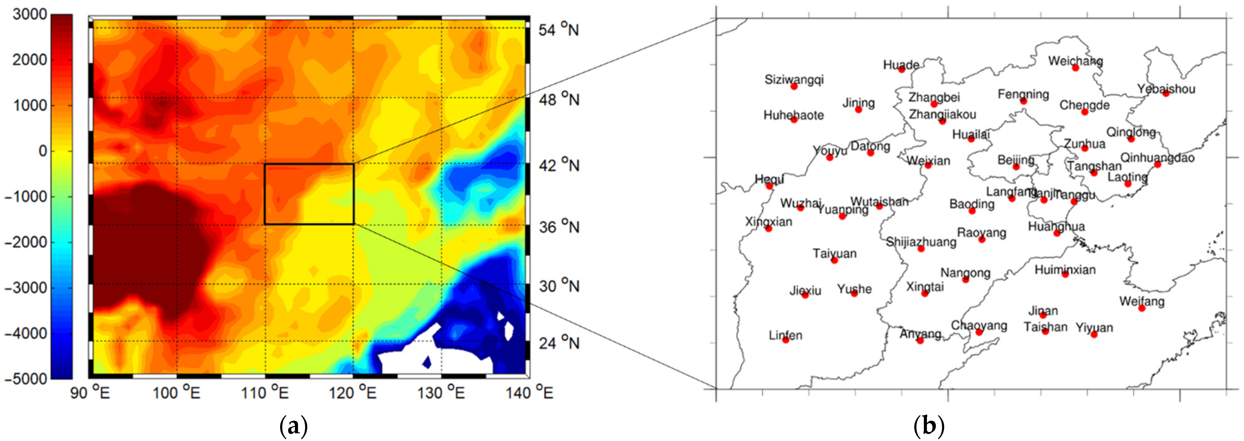
North China is located at the junction of Eurasia and the Pacific Ocean at mid-latitude, and the Tibetan Plateau, the highest altitude in the world, is located to its southwest (Figure 1a). The summer precipitation in North China is affected by the combination of low, middle, and high latitudes, as well as the plateau and the ocean, and the influence factors are complex and difficult to predict. Precipitation in North China generally decreases from south to north, and precipitation is uneven in all seasons, with the main precipitation concentrated in summer. In general, precipitation resources are abundant in the southern part of North China and relatively short in the northern part of North China. In this paper, we focus on the range of longitude from 111 to 120° E and latitude from 36 to 42° N (Figure 1b). The study area covers Beijing, Tianjin, Hebei, Shanxi, Inner Mongolia, and Shandong.
2.2. Data
2.2.1. Station Precipitation Data
The daily precipitation of the 721 weather stations in China during 1981–2010 is provided by the China Meteorological Administration. After comparison and screening, 45 stations were selected for the downscaling study in this paper, whose daily precipitation observations were provided by the Meteorological Information Center of China Meteorological Administration at www.cdc.gov.cn (accessed on 10 August 2019). In this paper, a 30-year time series (1981–2010) was selected among them, and 0.1 mm/day was used as the differentiation threshold between days with and without rain.
2.2.2. Reanalysis Data
In the downscaling modeling, in order to obtain more accurate relationships between atmospheric circulation and ground observations, statistical downscaling models are generally built using climate element fields from reanalysis data and precipitation data from local stations first, and then the model forecast factors are projected into the built model for simulation and prediction. In the selection of climate element fields, we should consider selecting some climate variable fields from the reanalysis data that have an obvious physical connection with local precipitation and can be simulated by the global model. Therefore, the developed model can be used in the downscaling work of the climate model in the future. Nine climate variable fields are selected as alternative forecasters, namely: 10 m Surface wind field (uas, vas), 500 hPa wind field (ua500, va500), 850 hPa relative humidity (hur850) and specific humidity (hus850), 10 m surface air temperature (tas), 850 to 500 hPa vertical decreasing rate of temperature Lapse rate, and sea level pressure (slp). There are obvious physical links between these forecast factors and local precipitation, among which, the wind field at different heights can characterize the lower atmospheric convergence and upper atmospheric dispersion, the humidity field and surface temperature field can characterize the water vapor condition and its saturation degree, the Lapse rate of temperature vertical decrement from 850 to 500 hPa can characterize the degree of atmospheric instability stratification, and the sea level pressure field can characterize the large scale. In addition, the sea level pressure field can characterize the large-scale circulation situation. These data are provided by the National Center for Environmental Prediction/National Center for Atmospheric Research (NCEP/NCAR) [20] (archived by the NOAA at https://psl.noaa.gov/data/gridded/data.ncep.reanalysis.html, accessed on 10 August 2019) on a daily basis (resolution 2.5° × 2.5°). Then, the fields of these variables are considered together as comprehensive elements describing the atmospheric state. Moreover, their correlation with precipitation at the station is calculated and judged as a condition for selection as a forecast factor. After this selection, the forecasting factor of precipitation at the target station can be used for SOM training.
2.2.3. Division of Time Periods
The first 20 years (1981–2000) were used for the establishment of the downscaled precipitation model, referred to as the downscaled model rate period, and the last 10 years (2001–2010) were used for the testing of the downscaled precipitation model, referred to as the downscaled model testing period.
2.3. Data Pre-Processing
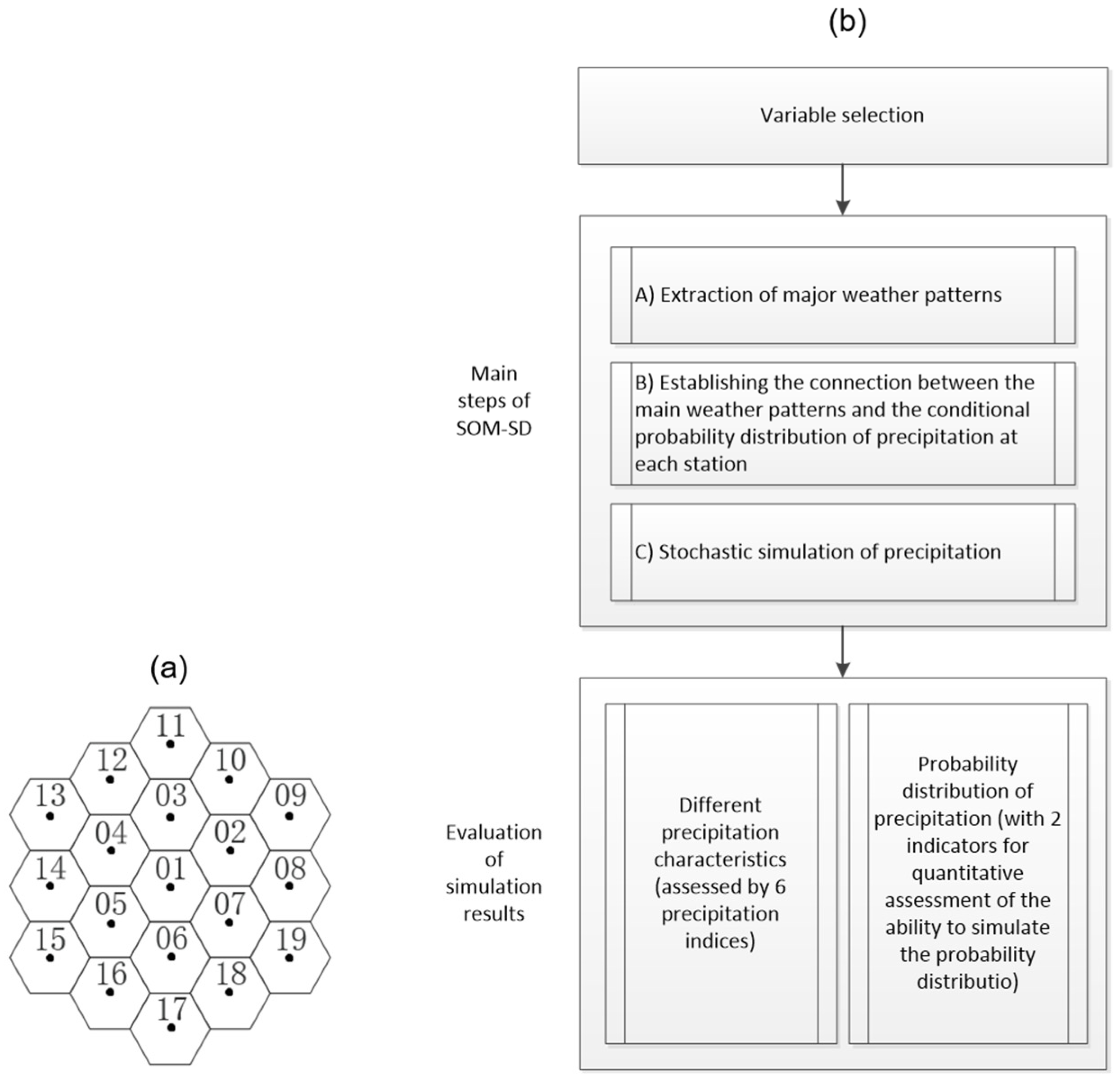
In order to be able to reflect the atmospheric state around the target station, the data can be preprocessed according to the method proposed by [24] for the grid information before downscaling: For each station, the n variable fields around the station can be described by n 1 × 19 vectors (Figure 2a).
As shown in Figure 2a, point 01 is the location of the station, and a square hexagon with a side length of 1° is made at the center of this point. This square hexagon is extended outward in two circles. For each hexagon, six vertices can form six triangles. In addition, the value of each triangle vertex can be obtained by weighing the values of the four grid points around the vertex according to the distance and by calculating the six triangle centers of gravity, respectively. Then, the value of the center of each hexagon is obtained by averaging the values of the six centers of gravity. The center of each hexagon represents the interpolation result of a climate variable in the region, and there are 19 points including the center point 01. The data of these 19 points can form a 1 × 19 vector, which represents a new variable field describing the conditions around the station. The daily data of all climate variable fields in a given time range are divided into seasons to form the input data for SOM training in the corresponding season.
3. Methods
In this paper, the method presented is rather complicated. To have a clear presentation, we have mapped out the most important steps (Figure 2b). The first step is the selection of variables, followed by the downscaling of precipitation, and finally the evaluation of downscaling simulation results.
3.1. Principles and Methods for the Selection of Predictive Factors
The selection of predictors is an important part of the downscaling process, and the usability of the downscaling results depends on the appropriateness of the selection of predictors. The selection of predictors is very complicated, for example, some predictors are very important but may have low explanatory power for the forecast objects, and the explanatory power of each predictor may change with time and space [13,25,26].
The Spearman rank correlation coefficient method is used in this paper. The reason for adopting this method is that the daily precipitation time series do not satisfy the assumption of normality of linear methods in previous studies due to their characteristics of non-negativity, many zero values, and non-normality. In contrast, various types of statistical forecasting models and statistical test methods, as well as the commonly used Pearson correlation coefficient calculation require the information to conform to a normal distribution. Common solutions are power transformation (cube root or quadratic root, etc.) normalization, hyperbolic tangent transformation normalization, setting certain thresholds to eliminate negative downscaling results, etc. However, these practices lack a physical basis [27] and some precipitation series still do not obey normal distribution after this treatment due to the high number of zero values.
In this case, the Spearman rank correlation coefficient can be considered for the forecaster preference. This correlation coefficient has the advantages of not requiring the data to obey a normal distribution, good robustness, and insensitivity to outliers. When the data series do not obey a normal distribution, have poor quality or are suspected to be affected by outliers, it is more reasonable to use the rank correlation coefficient compared to the Pearson correlation coefficient.
3.2. The Main Implementation Steps of the SOM-SD Model
The SOM-SD model consists of three main steps: First, the SOM technique requires training of the preferred forecasters to identify all of the possible weather patterns around the target station. Second, the observed precipitation sequences are grouped into different sets of precipitation values according to the category number of the clustering results, and each set of precipitation values corresponds to a weather pattern, thus establishing the association between the forecasters and the precipitation. Third, the forecast factors of each day are projected into the SOM nodes obtained from the training, and the precipitation values are randomly selected from the set of precipitation values corresponding to the class according to the category number of the projection result. The following is a detailed description of the three main steps of downscaling for one station, and the rest of the stations in the study area adopt the same process to realize their own downscaling.
3.2.1. Obtaining Various Weather Patterns That Represent the Atmospheric State around the Station through SOM Clustering
The SOM training is performed on the preferred forecast factors of 19 grid points around the station to obtain a set of ordered two-dimensional nodes, each of which can represent a weather pattern. Then, the daily multivariate climate variable field is mapped to one of the SOM nodes to identify the category of weather patterns around the target site each day. Among them, the number of nodes is an optional value, and the number of SOM nodes selected varies among studies in different regions in the past [14,15,28,29]. This is somewhat subjective and care needs to be taken when determining the number of nodes: If the number of nodes is too small, it will increase the generality of the categories and the differentiation of different weather states will be reduced. If the number of nodes is too large, the number of samples assigned to each node is too small to facilitate the estimation of precipitation downscaling values at a later stage. However, after repeated tests and comparisons, it is found that the number of nodes does not have a significant effect on the downscaling effect. In this paper, we do not analyze in depth the degree of influence of the change of SOM node size on the downscaling results, and only take the SOM output node size of 4 × 4 as an example for analysis.
3.2.2. Establishing the Relationship between Station Precipitation and Weather Patterns around the Station
After the SOM training is completed, the relationship between station precipitation and weather patterns can be established. The time period used for model establishment can be called the rate period of the model, and the time period used for model testing can be called the testing period of the model. For each day of the model rate period, its forecast factor can be compared as a sample with the nodes obtained from SOM training (calculating the Euclidean distance between them), and the one with the shortest Euclidean distance can be selected based on the calculation of the Euclidean distance, i.e., the winning node. Then, the precipitation value corresponding to that day is projected to the winning node, and that precipitation value can be assigned to a class according to the serial number of the winning node. The above process is repeated until all of the precipitation values are classified, in order that the precipitation values are also classified into corresponding groups according to the SOM nodes, and each group of precipitation values corresponds to one SOM node.
Each precipitation value is related to the corresponding weather pattern (SOM node) in this way. Since each node represents a different atmospheric state, the precipitation probability density curves plotted with the set of precipitation values corresponding to each node also vary, i.e., the probabilities of precipitation values that can be produced by different natures of weather patterns are different. In addition, this correspondence between precipitation values and weather patterns can be well captured by projection. In this paper, we use the Gamma distribution in each category of precipitation values to fit the precipitation probability density function in order to obtain the fitted parameters of the probability density function for each category. Then, we use the fitted parameters of the obtained probability density function to generate random precipitation values in the next step of the downscaling process.
3.2.3. Obtaining Downscaled Precipitation Series Based on Monte Carlo Simulation
By projection, the relationship between precipitation values and weather modalities is established. Next, the validation data of the model testing period can be used to evaluate the downscaled model simulation results. For each downscaled target station, its forecast factors are compared with the trained SOM nodes one by one, and the corresponding node class number of each day can be obtained, through which the forecast factors of each day are related to the corresponding set of precipitation values. Then, the corresponding precipitation value for a particular day can be generated from a certain set of precipitation values by random resampling, which is generated according to the parameters of the fitted probability density function. Precipitation values for all of the days of that time period are generated in this way, and a precipitation downscaling time series can be formed.
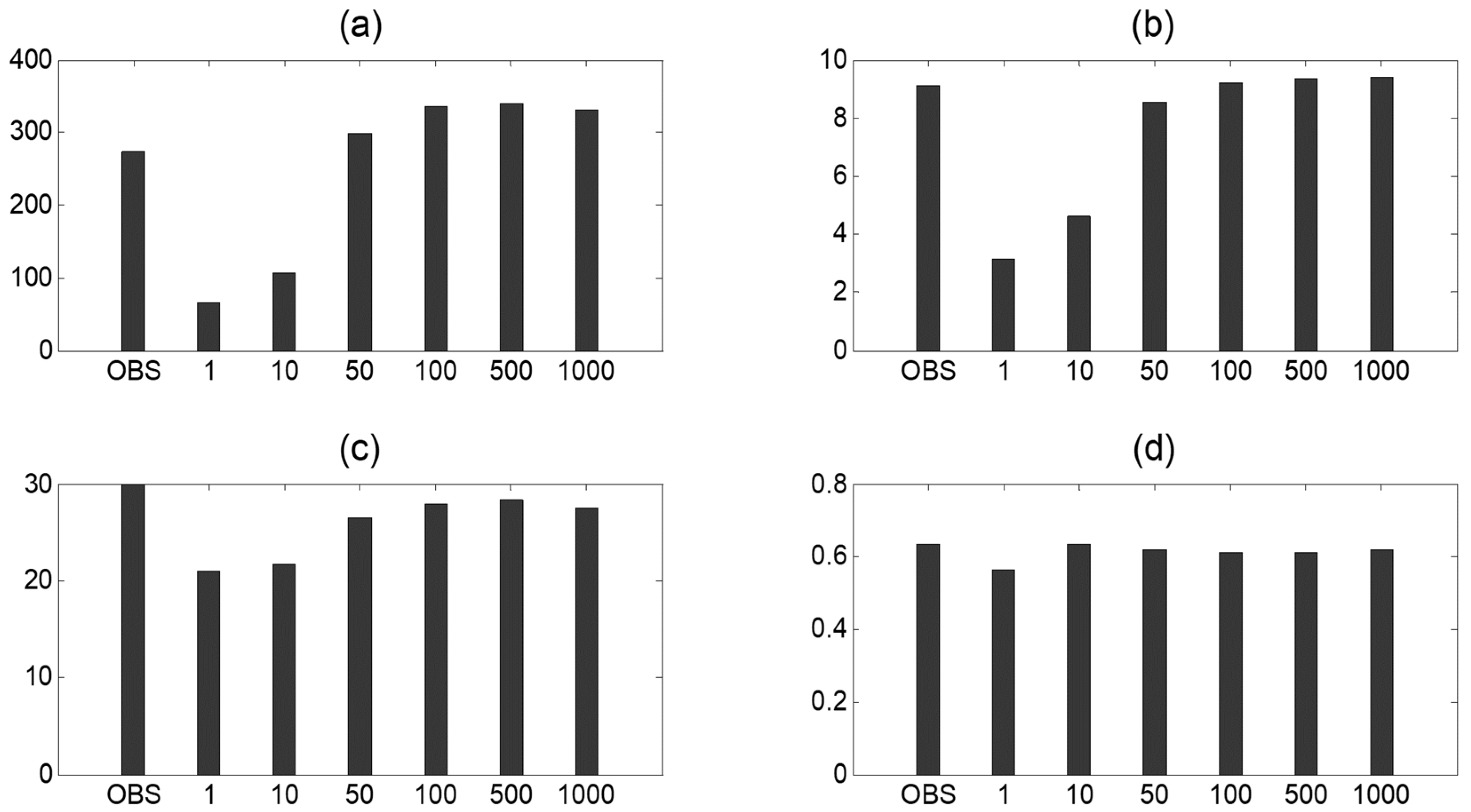
In the random generation of the precipitation downscale sequences, the random resampling of the downscale results was repeatedly tested and compared several times in order to be able to reflect the probability distribution characteristics of the precipitation downscale database to the maximum extent. Each generated sequence of equal length to the observed value sequence is considered as a sample in the precipitation database. To test whether the downscaled results gradually stabilize with the increasing sample size, several different metrics (Prtot, SDII, nr001, P95T, etc.) can be used. The results are plotted here for 1, 10, 50, 100, 500, and 1000 times (Figure 3).
In Figure 3, as the number of resampling increases, each indicator value gradually converges with the observed value results and gradually stabilizes. As the number of resampling reaches 1000 times, the above time series are repeated 1000 times to obtain 1000 simulated series of precipitation downscaling of equal length with the station observation series of precipitation.
3.3. Methodology for Evaluating the Simulation Capability of the SOM-SD Model
3.3.1. Evaluation Index of the Degree of Error of the Probability Density Function
To quantitatively analyze the simulation performance of the SOM-SD model for the probability density function (PDF) of precipitation at each station, the Brier Score () [30] and the Significance Score () [31,32] based on the probability density function can be used to evaluate the degree of error between the simulated and observed probability density functions.
where n denotes the probability density function divided into n equal length intervals, and and are the values of the probability density functions of the observed and simulated variables in the interval, respectively. is a measure of the non-coincidence between the observed and simulated probability density functions, and the smaller the non-coincidence, the closer the value of the index is to zero, which indicates the better the simulation result. reflects the area of the mutual overlap between the simulated and observed probability density functions of the two series. The larger the overlapping area is, the larger the value is, and it reaches the maximum value of 1 when they completely overlap. Therefore, the closer the value of this indicator is to 1, the better the simulation result.
3.3.2. Evaluation Index of Statistical Characteristics of Daily Precipitation Statistical Downscaling Results
In this paper, to observe the statistical characteristics of the daily precipitation statistical downscaling results, some commonly used precipitation indices are selected (the specific meaning of each indicator is detailed in Table 1). In addition, most of these indicators are selected from the core indicators of the EU STARDEX program for analyzing extreme climate events (http://www.cru.uea.ac.uk/cru/projects/stardex/, accessed on 10 August 2019). They mainly include the following: Total season precipitation (Prtot), daily precipitation intensity (SDII), mean number of precipitation days (nr001), percentage of rainfall from events beyond 95th percentile value of overall precipitation (P95T), maximum consecutive wet days (CWD), and maximum consecutive dry days (CDD).
4. Application of SOM-SD Model in North China
4.1. Selection of Prediction Factors
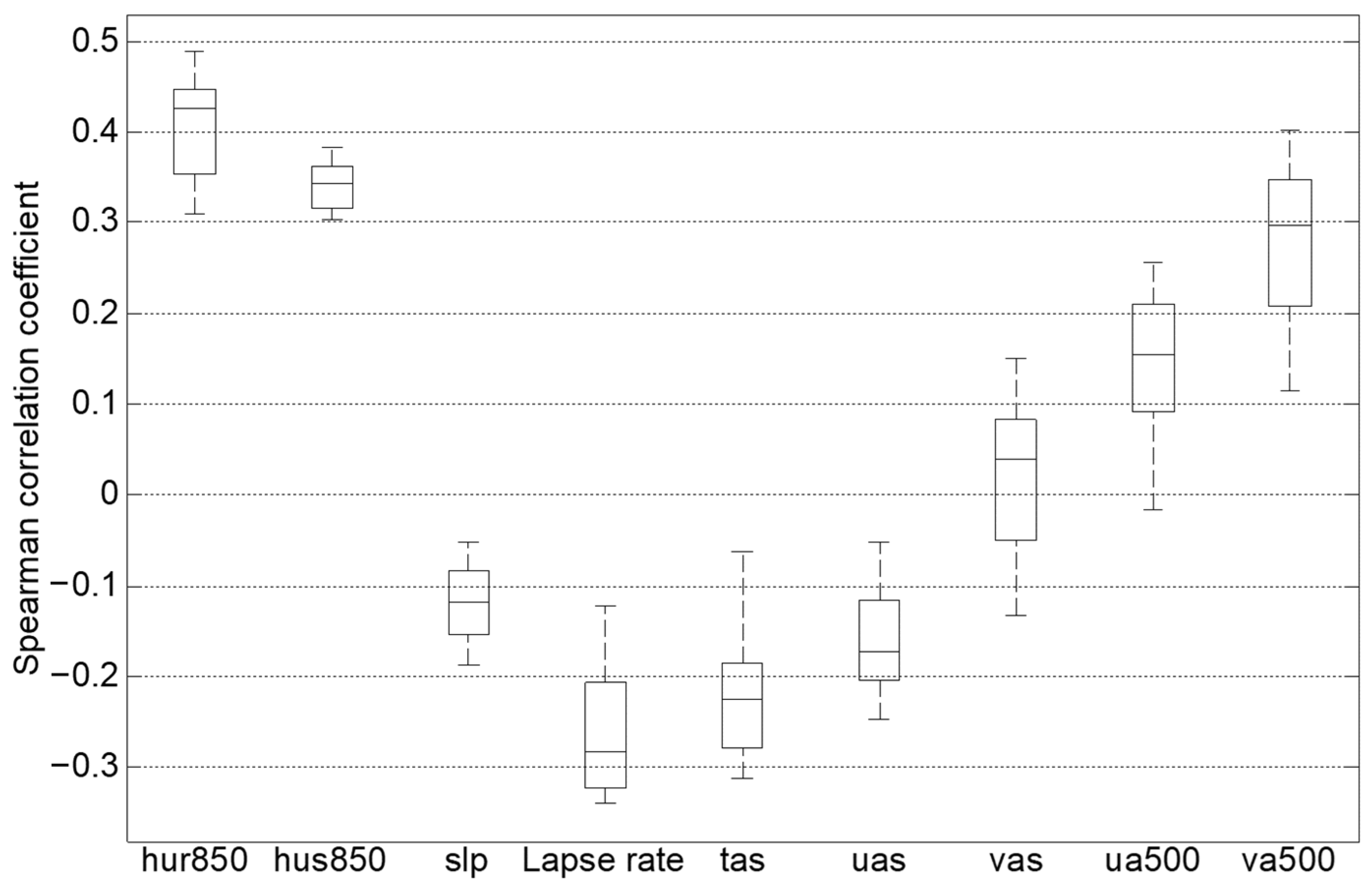
For each station, each alternative predictor (hur850, hus850, slp, Lapse tate, tas, uas, vas, ua500, va500) is interpolated into 19 grid points around the station by a bilinear interpolation method (as shown in Figure 2a). In this way, each predictor can form a time series at each grid point separately (19 × 9 = 171 time series in total for the nine predictor fields). Then, the Spearman correlation coefficients are obtained for each of these predictor time series with the station precipitation time series and tested for significance. The correlation coefficient is useful to measure the degree of correlation between two factors in an objective way. As an example, the results are plotted in Figure 4 for the Beijing station.
In Figure 4, the horizontal axis shows the nine predictors and the vertical axis shows the Spearman correlation coefficients of each predictor with the precipitation series R. The horizontal line in the middle of the box represents the median of the data. The two lines above and below the box are the upper and lower quartiles of the data, respectively. The gap between these two lines is the height of the box. It reflects the fluctuating state of these data. The flatter box indicates a more concentrated data distribution. The upper and lower edges of the outstretched whiskers generally represent the maximum and minimum values of the data. In addition, the shorter the outstretched whiskers, the more concentrated the data. From the figure, we can see that the predictors hur850, hus850, ua500, and va500 have a positive correlation with precipitation. The remaining forecast factors, except vas, all have negative correlations with precipitation (slp, lapse rate, tas, and uas). The above results indicate that in Beijing, the low-level humidity field is more closely related to summer precipitation and can provide sufficient water vapor supply, which is one of the key factors affecting summer precipitation. The smaller the vertical decreasing rate of temperature, the more unstable the atmosphere is, and the more obvious the vertical motion is, which is also more closely related to summer precipitation. The lower the air pressure around the station, the more favorable the formation of precipitation. The trend of surface air temperature and precipitation is also inverse, as the solar radiation absorbed by the ground decreases in rainy weather in summer, and the surface air temperature decreases accordingly.
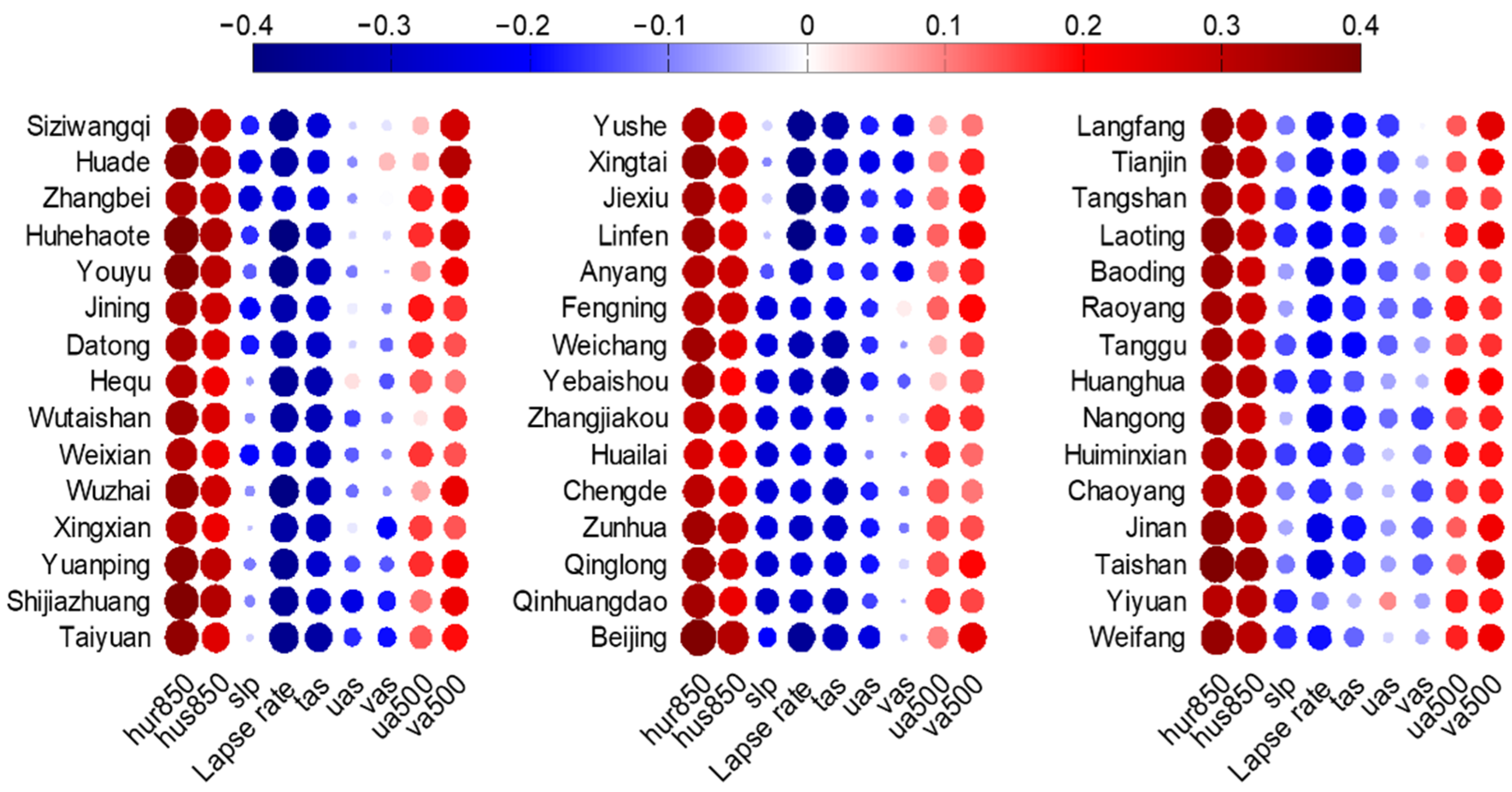
The Spearman correlation coefficients are calculated for the remaining stations according to the same calculation method, and Figure 5 shows the results of the correlation coefficients. In Figure 5, the red color indicates a positive correlation and the blue color indicates a negative correlation. From Figure 5, we can see that forecast factors, such as hur850, hus850, ua500, and va500 are significantly positively correlated with precipitation at most of the stations, while forecast factors, such as lapse rate and tas are significantly negatively correlated with precipitation at most of the stations. The above results show that for different meteorological conditions, the effect of slp, uas, and vas on precipitation is relatively weak.
The above results indicate that the relationship between each meteorological element and summer precipitation varies somewhat for different meteorological stations. Prior to downscaling, it is necessary to optimize the forecast factors for different stations, in order to better reflect the atmospheric conditions around the stations.
4.2. Analysis of Precipitation Characteristics at Different Nodes of SOM
4.2.1. Cumulative Probability Distribution Function CDF Curves of Precipitation Values Corresponding to SOM Nodes
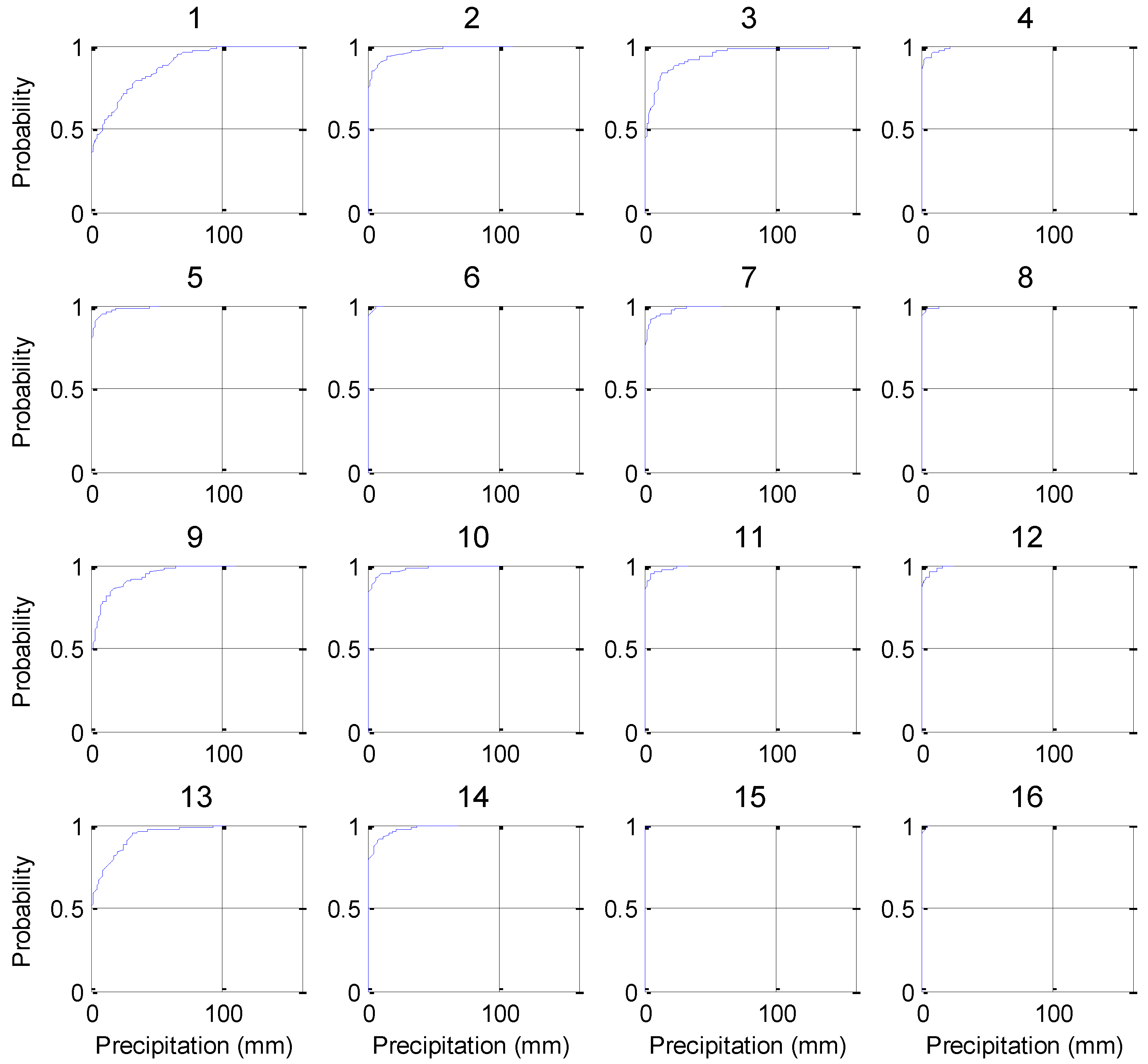
Figure 6 shows the CDF curves of the cumulative probability distribution of daily precipitation corresponding to the 16 SOM nodes. The cumulative probability distribution curves of precipitation from node 1 to node 16 show a strong regularity: There is a clear pattern of gradually decreasing precipitation along the diagonal line (from the upper left to the lower right). For the nodes corresponding to the atmospheric states favorable to precipitation formation (e.g., nodes 1, 2, 5, and 6), the corresponding precipitation CDFs show larger precipitation values. On the contrary, for the nodes corresponding to unfavorable precipitation generation (e.g., the 11th, 12th, 15th, and 16th nodes), the corresponding precipitation CDFs show smaller or close to zero precipitation values. The above results show that there are significant differences in the CDF curves in different SOM nodes. This implies that important differences in different precipitation conditions have been accounted for in the clustering of weather patterns using the SOM method. In the context of weather-scale circulation, this difference in the CDF curves in different SOM nodes has some physical implications, i.e., a correspondence between precipitation and circulation fields has been established.
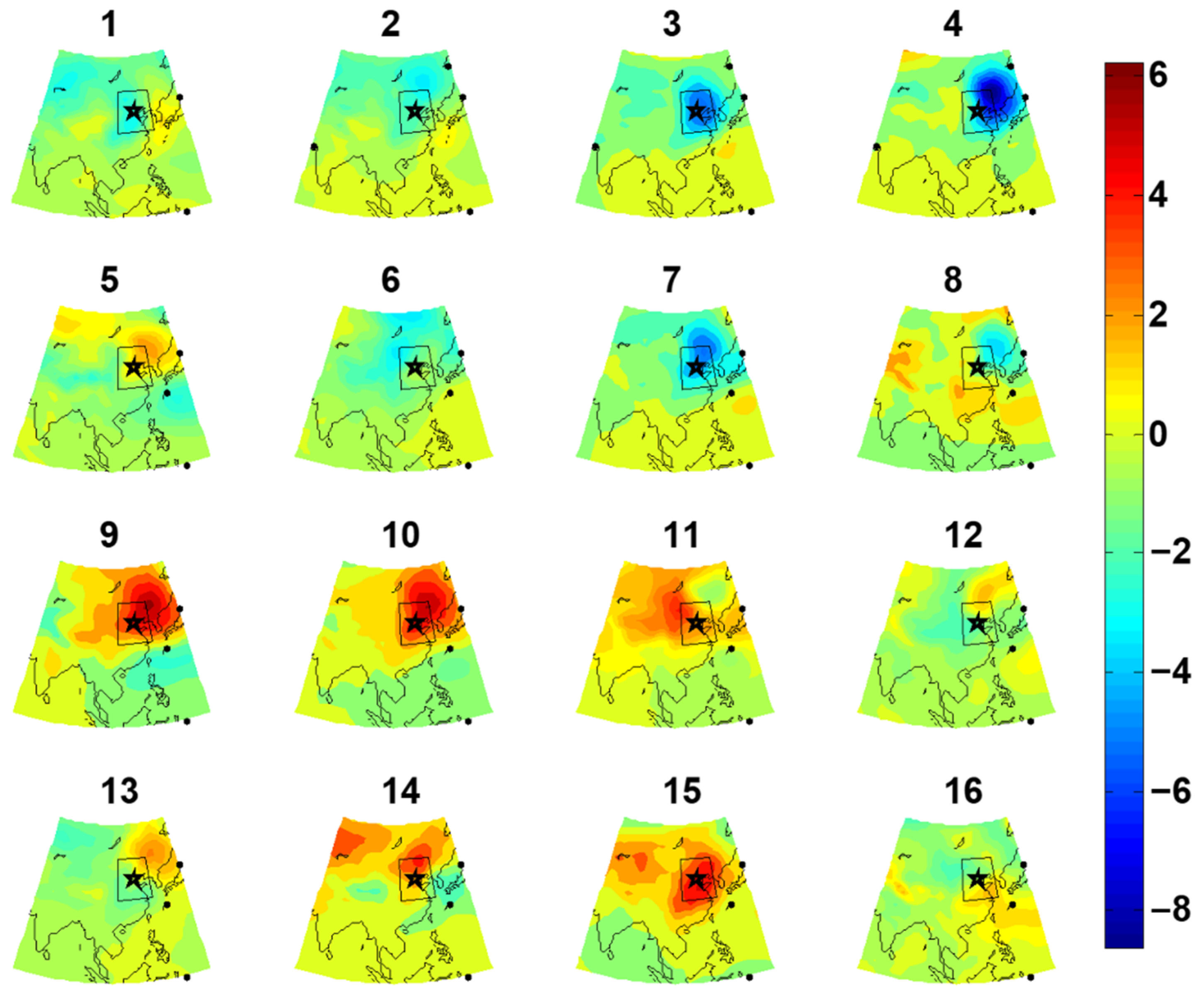
To observe the circulation fields corresponding to the 16 SOM nodes and analyze their distribution patterns, the node distribution of each forecast factor can be plotted separately for the analysis. Considering the complexity of the causes of summer precipitation, in addition to the small and medium rainfall, the more important summer precipitation is heavy rainfall due to strong convective weather, while most of the heavy rainfall is not caused by atmospheric circulation anomalies. In addition, the dominant factors inducing summer rainstorms should be humidity and temperature, which tend to cause atmospheric instability, and thus, favor the formation of precipitation. The distance level fields of two representative variables, 850 hPa relative humidity (hur850) and 850 to 500 hPa vertical decreasing rate of temperature (Lapse rate), are plotted below for the analysis (see Figure 7 and Figure 8).
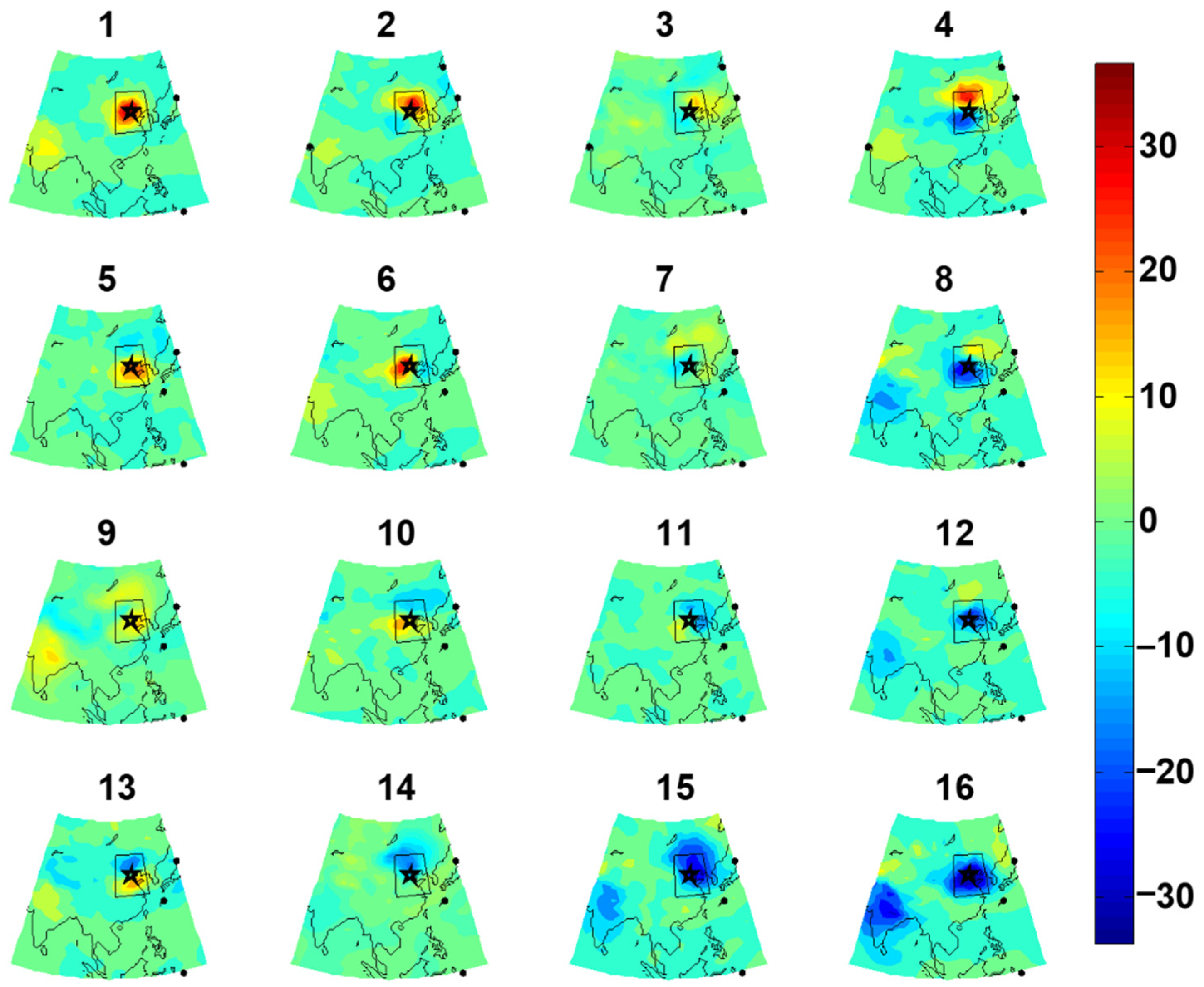
Figure 7 shows the node distribution of the 850 hPa relative humidity (hur850) pitch level field. In the figure, there is a positive pitch level center of relative humidity in the top left corner of nodes (1), (2), (5), and (6) that precisely surround Beijing station, which corresponds to the wet node in Figure 6. In addition, the nodes (11), (12), (15), and (16) in the lower right corner all have a negative pitch level center of relative humidity exactly around Beijing station. This corresponds to the dry node in Figure 6. Figure 7 is more consistent with the distribution pattern of the nodes in Figure 6, indicating that 850 hPa relative humidity is an important factor affecting precipitation and needs to be considered when downscaling. In addition to the relative humidity field, the specific humidity field (not shown) shows a similar pattern. Therefore, the specific humidity is also an important factor affecting summer precipitation and should be selected when performing variable preferences.
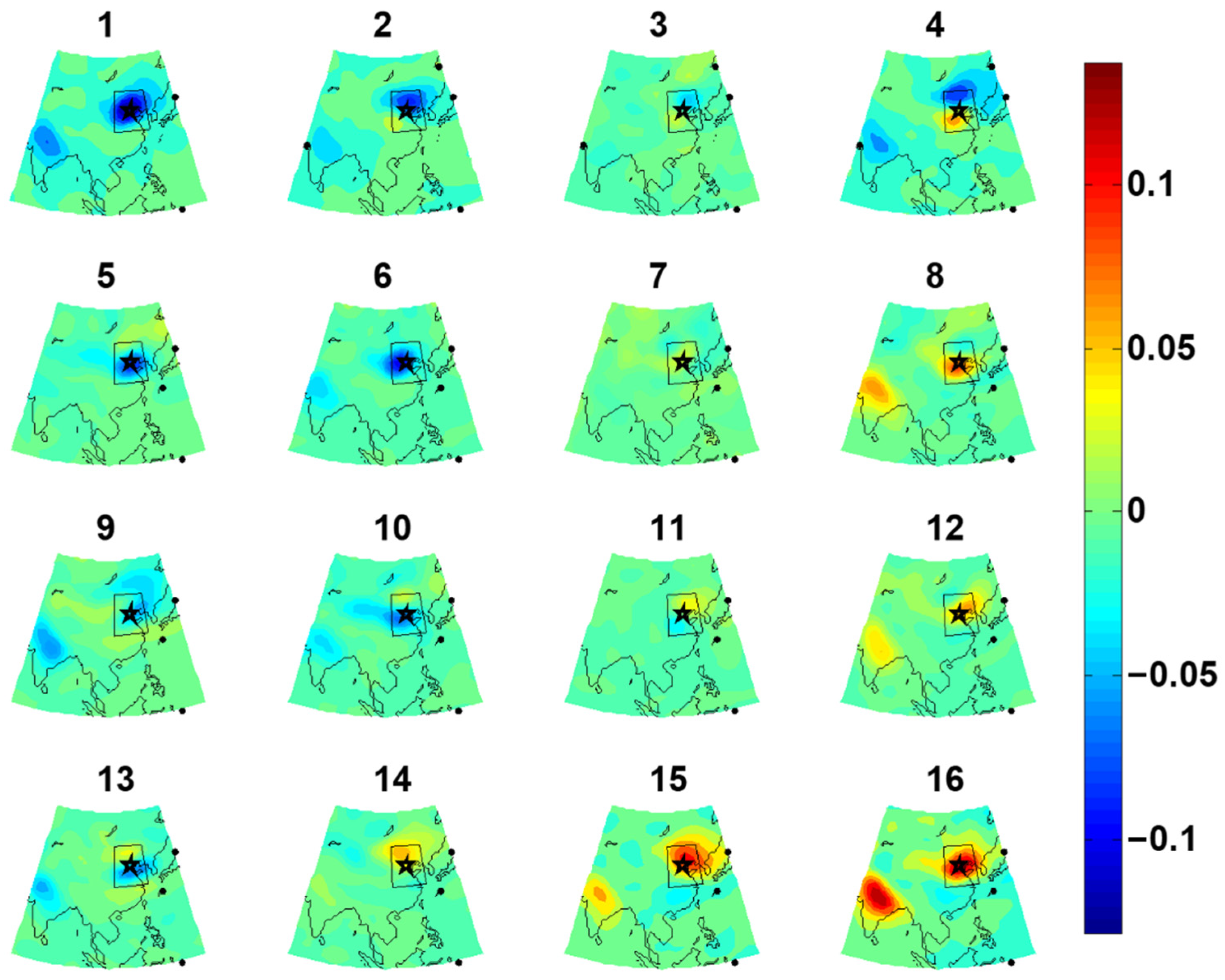
In Figure 8, the node distribution of the vertical decreasing rate (Lapse rate) of temperature from 850 to 500 hPa is plotted in the distance level field. The distribution also has a more obvious distribution pattern from the upper left corner to the lower right corner. In the upper-left corner, the negative pitch level surrounds the Beijing area, which corresponds to the node with large values of precipitation (i.e., wet node). In the lower-right corner, the positive pitch level surrounds the Beijing area, which corresponds to the node with small values of precipitation (i.e., dry node). It is shown that the vertical decreasing rate of temperature (Lapse rate) from 850 to 500 hPa is also an important factor affecting the summer precipitation.
To observe the relationship between the circulation field and station precipitation, the sea level pressure (slp) distance level field is plotted in Figure 9. If slp is closely related to precipitation, the arrangement of SOM nodes should have the following pattern: Nodes that are relatively close to each other and nodes that are opposite in nature are arranged far away from each other. For the slp field, the node in the upper left corner (1) should be low-pressure dominant (indicated in blue), while the node in the lower right corner (16) should be high-pressure dominant (indicated in red), and the rest of the nodes gradually transition from high to low. However, the results of the slp field shown in Figure 9 do not fully follow this pattern. They indicate that among the influencing factors of summer precipitation, the slp field is not the most closely related to precipitation. The results also show that in some cases where high pressure prevails, precipitation may also be formed due to atmospheric instability, and in some cases where low pressure prevails, precipitation may not be formed due to lack of water vapor. Therefore, the causes of summer precipitation cannot only consider the circulation field, but need to consider more meteorological elements together.
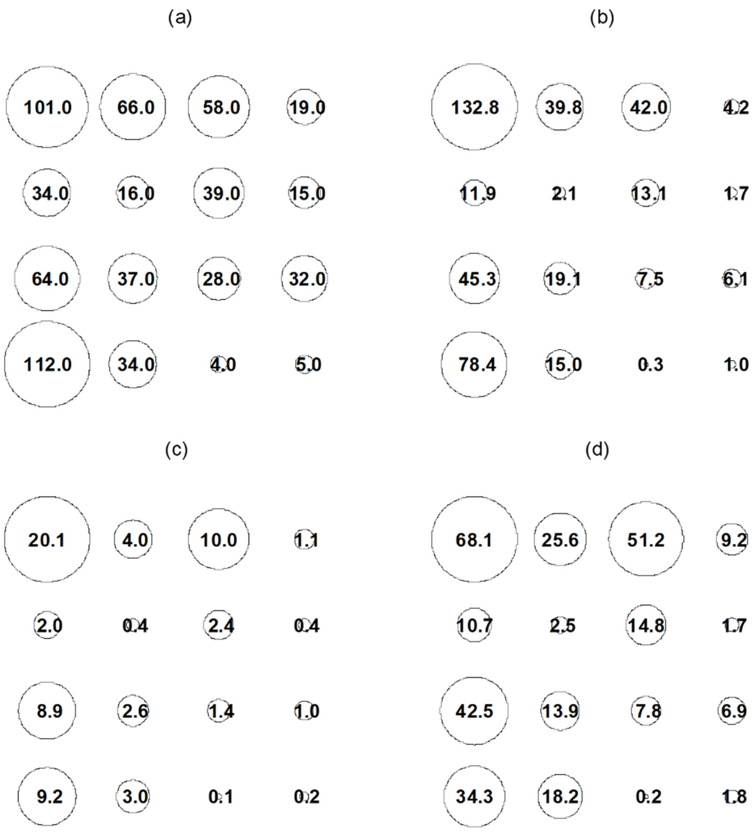
Further analysis and validation are needed to determine which of these nodes are more likely to form precipitation. The number of rainy days, total precipitation, average daily precipitation, and 95th percentile precipitation values of precipitation in each node were counted separately, and the results are plotted in Figure 10.
From Figure 10, it can be seen that the 1st node has 101.0 days of rain, 132.8 mm of annual average total precipitation, 20.1 mm/day of daily average precipitation, and 68.1 mm of 95th percentile precipitation value. In addition, the above indicators (frequency, total, average, and extreme) show the maximum value among all of the nodes many times, thus it can be defined as a wet node. On the contrary, the 15th node shows less precipitation in each of the above indicators and can be defined as a dry node. The rest of the nodes can be considered as transition nodes.
The significant difference between the CDF curves of the dry and wet SOM nodes indicates that the SOM clustering results of atmospheric states can, to a certain extent, distinguish different precipitation scenarios at different weather scales (different atmospheric states bring different levels of precipitation). This result fully demonstrates the advantages of SOM clustering: (a) When there are many forecast factors and the relationship with precipitation is non-linear, the clustering can be successfully achieved using SOM. (b) SOM can cluster different atmospheric states into nodes of a different nature, and different nodes bring different magnitudes of precipitation. (c) The results of clustering are continuous as a whole, and the evolution of different nodes can be easily observed in a visualized form. (d) The distribution of dry and wet nodes exhibited in the clustering results is very clear. The distribution pattern of different factors in the same mode can be observed on this basis.
4.2.2. Distribution Patterns of Different Factors in the Same Type
A detailed comparison and analysis of each predictor is required to determine the state of each predictor in the wet node, and whether the combination of these predictors can describe a particular atmospheric state and estimate the probability distribution of precipitation in that atmospheric state.
To visualize the distribution characteristics of each variable field in each atmospheric state (represented by a certain SOM node), the fields of each variable in the two diametrically opposed nodes, dry and wet, are plotted separately in order to analyze the main causes of changes in precipitation values.
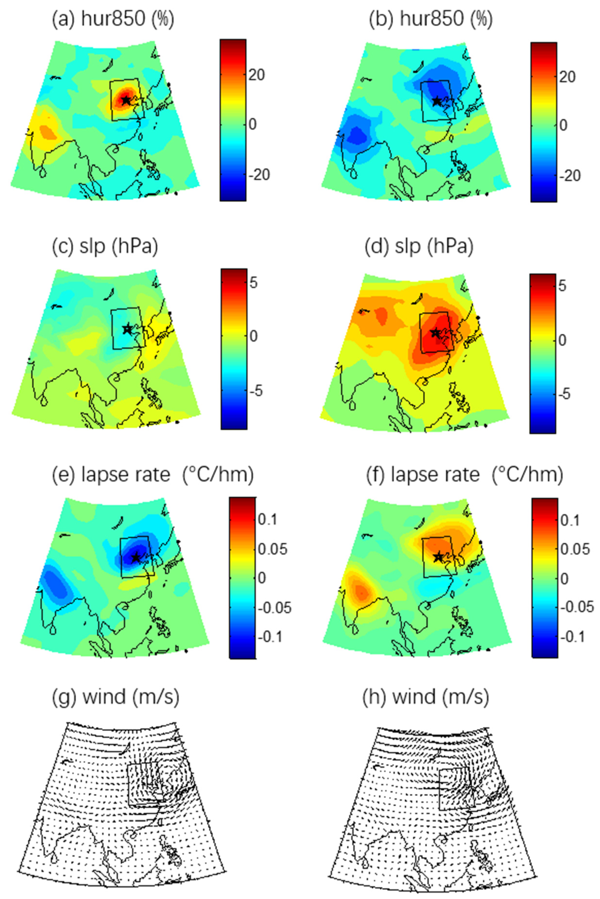
In Figure 11, the distribution states of each predictor in the wet and dry nodes are compared, where the left column figures show the spatial distribution states of the distance level field of each predictor in the wet nodes. It can be seen that in the wet node (Figure 11, column 1), the 850 hPa relative humidity (hur850) is at a positive distance level, which is significantly positively correlated with precipitation, while the 850 to 500 hPa vertical decreasing rate (Lapse rate) is at a low value, which is significantly negatively correlated with precipitation. This indicates that both variables have a good relationship with precipitation. In this state, sufficient water vapor can be provided to Beijing station, which is conducive to the formation of precipitation. The state of each variable in this node near Beijing Station is the most likely state to bring precipitation, and the possibility of bringing more precipitation is high. In the dry node (Figure 11, column 2), the 850 hPa relative humidity (hur850) is basically close to or at a negative pitch level around Beijing, while the vertical decreasing rate of temperature (Lapse rate) from 850 to 500 hPa is basically close to a high value. It cannot provide a sufficient water vapor source for Beijing station, which is not conducive to precipitation formation.
The 500 hPa wind field distance level is plotted in Figure 11g,h, where Figure 11g shows the 500 hPa wind field distance level in the wet node, and Figure 11h shows the 500 hPa wind field distance level in the dry node. In Figure 11g, the 500 hPa wind field pitch level rotates clockwise with the Korean Peninsula as the center, and the wet airflow turns northward after landing westward in the eastern coastal area of China, which can bring sufficient water vapor to the Beijing area. In Figure 11h, the 500 hPa wind field level has a central point near Mongolia, and the wind field level rotates clockwise around this point. The dry airflow near Beijing is mainly from the north, and this airflow cannot bring the necessary water vapor for precipitation when it goes south through Beijing. Therefore, there are no precipitation conditions.
The above analysis shows that several forecast factors, such as the 850 hPa relative humidity (hur850), 850 to 500 hPa vertical decreasing rate (Lapse rate) and 850 hPa specific humidity (hus850) (not shown), 10 m surface air temperature (tas) (not shown), 500 hPa wind field (ua500, va500), are the main forecast factors affecting precipitation in the dry and wet nodes. Moreover, due to the fact that the states of each forecast factor in the dry and wet nodes are diametrically opposed, this brings different precipitation.
4.2.3. Analysis of the Relationship between Interannual Variation of Wet and Dry Node Frequency Difference and Interannual Variation of Average Daily Precipitation
The trend of its frequency difference (wet node frequency minus dry node frequency) will better reflect the change of precipitation compared to the trend of wet node or dry node frequency. If the frequency difference increases upward, it already contains the following situations: The wet node frequency remains unchanged and the dry node frequency decreases; the wet node frequency increases and the dry node frequency remains unchanged; the wet node frequency increases while the dry node frequency decreases. Moreover, if it increases in the same direction, the wet node frequency increases more; and if it decreases in the same direction, the dry node frequency decreases more. In other words, the model does not need to well simulate the frequencies of both wet and dry nodes. As long as the difference between the frequencies of the two is well simulated, it can reflect the changing trend of precipitation. According to this law, the future precipitation prediction can be corroborated from a new perspective, whether the future precipitation prediction is credible or not.
To test the reasonableness of the above hypothesis, the year-by-year dry and wet nodal frequency differences at each node of Beijing station were counted, and the summer average daily precipitation at the station was also counted year-by-year. The calculated results show the following pattern: The frequency difference between the wet and dry nodes also shows a similar trend, and the correlation coefficient between them reaches 0.54 (at the 95% confidence level).
The above results indicate that the change of the frequency difference between wet and dry nodes at Beijing station does affect the change of precipitation. To test the universality of this law in the remaining stations in North China, similar calculations were performed for the rest of the stations, and the average correlation coefficient of the 45 stations was 0.41 (at the 95% confidence level), indicating the universality of this law. There is a significant positive correlation between the interannual variation of the difference between the occurrence frequency of the wet and dry nodes and the interannual variation of precipitation. The trend of precipitation can be estimated from the variation of dry and wet nodes.
4.3. Simulation Test of SOM-SD Model in North China
The previous analysis has demonstrated that weather variability can be captured using the SOM method, which portrays the atmospheric state represented by SOM nodes. In addition, different SOM nodes correspond to different precipitation characteristics, i.e., the CDF curves of precipitation are not consistent at different SOM nodes. Moreover, it is possible that different precipitation amounts may be brought at the same node (with similar atmospheric conditions). To capture this randomness, random repetitive sampling can be performed from the CDF curve of each node to ensure that the downscaling results can match the statistical characteristics of the observed value series. Furthermore, the reasonableness of the dry and wet node definitions and the forecast factor preferences have been tested in the previous work. Next, it is necessary to check whether the trained SOM can be used to generate a precipitation daily time series, and whether the time series has a high agreement with the observed value series in terms of magnitude, frequency, and other characteristics, which can be judged by the evaluation of the precipitation downscaling results. The assessment of the effect of precipitation downscaling requires an examination of the statistical characteristics of the precipitation downscaling results in terms of precipitation quantity, precipitation frequency, and extreme precipitation.
4.3.1. Analysis of Simulation Results on the Probability Density Function of Downscaling Results
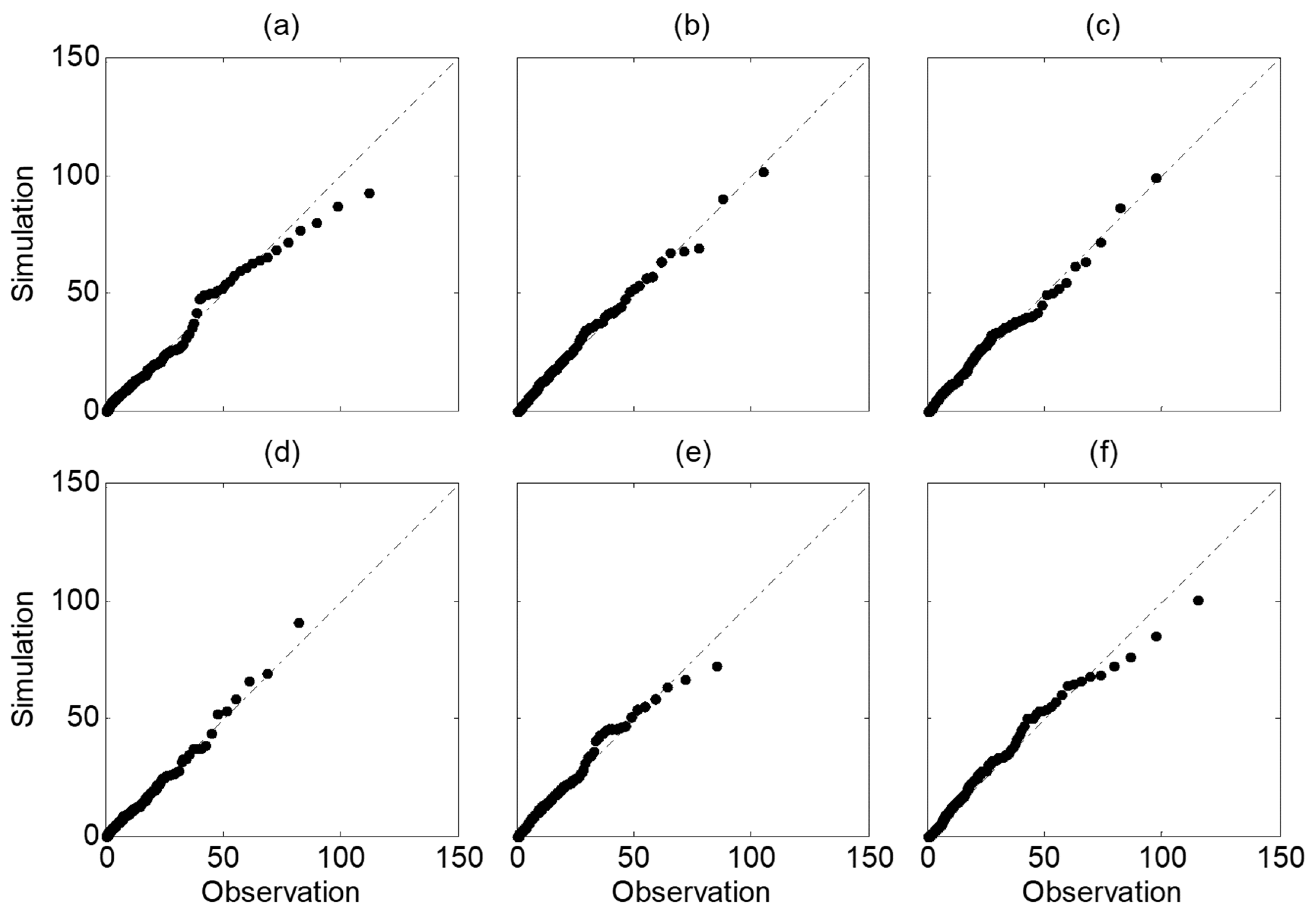
To observe whether the downscaled results can well reflect the probability density characteristics of the observed values, the Q-Q plots of the downscaled results of summer precipitation are plotted in Figure 12 (taking Beijing, Tianjin, Shijiazhuang, Hohhot, Taiyuan, and Jinan stations as examples). In Figure 12, the scatter points of precipitation basically fall on the diagonal line, indicating that the two obey a uniform distribution. The above results show that the downscaling results of the SOM-SD model can well reflect the probability distribution characteristics of summer precipitation in North China.
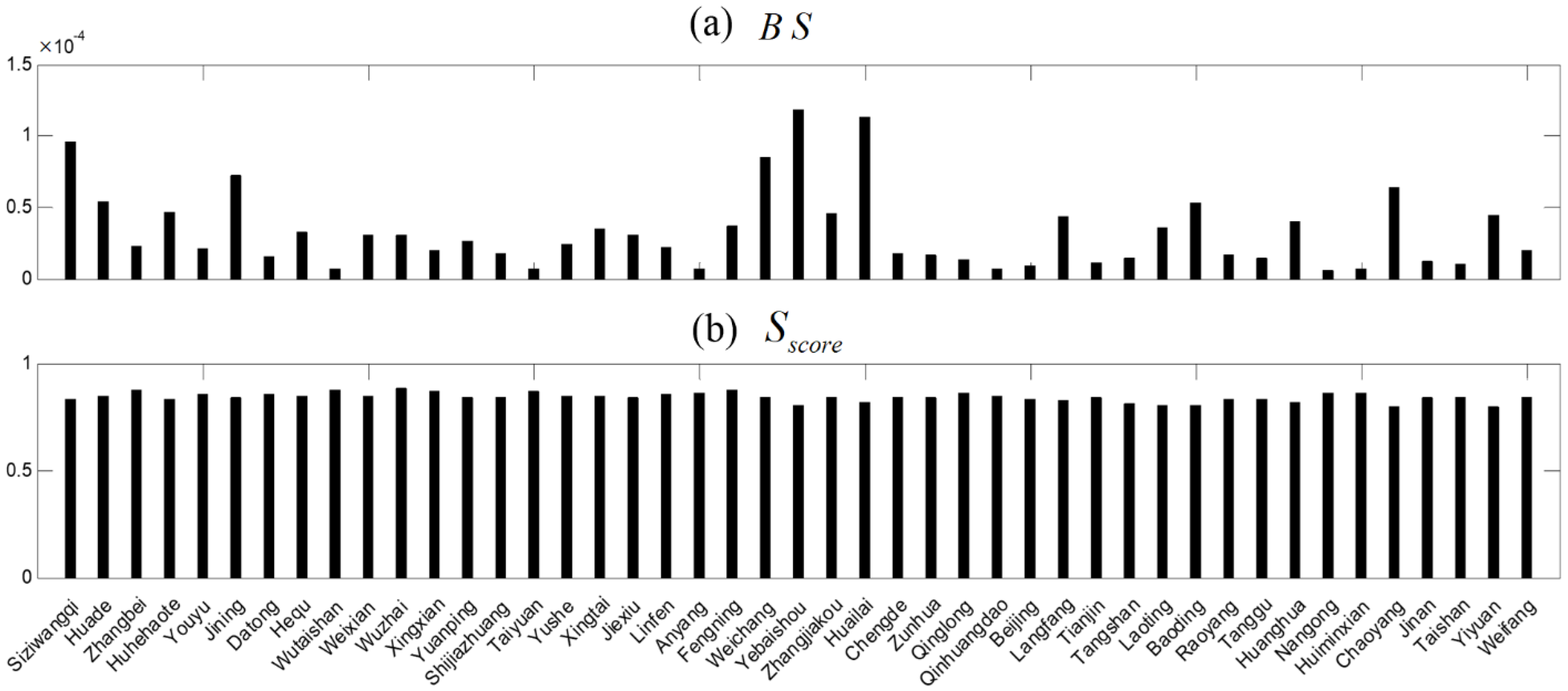
To quantitatively evaluate the ability of the downscaling model to simulate the probability density function of precipitation, two indicators, and , are used to evaluate the errors between the downscaled simulation results and the observed values at each station, and the results are plotted in Figure 13. The closer the value of the indicator is to 0 and the closer the value of the indicator is to 1, the better the simulation capability is. From Figure 13, the values of the indicators are in the range of 0 to 1.5 × 10⁻⁴ and the values of the indicators are in the range of 0.8 to 1, indicating that the SOM-SD model can well simulate the probability density function of summer precipitation in North China.
4.3.2. Evaluation of the Validity of the SOM-SD Simulation Results for Station Precipitation
To evaluate the applicability of the model for summer precipitation in North China more quantitatively, the total precipitation (Prtot), precipitation intensity (SDII), total number of rainy days (nr001), extreme precipitation contribution (P95T), maximum continuous rainy days (CWD), and maximum continuous rainless days (CDD) are used to evaluate the precipitation, precipitation frequency, and extreme precipitation, respectively. The simulation error (simulated value–observed value) and the error percentage ((simulated value–observed value)/observed value × 100%) need to be calculated. The observed and simulated values were first taken as regional averages at 45 stations, and then the simulated errors and error percentages were calculated. The comparison of the downscaled results with the observed values is listed in Table 2.
As can be seen from Table 2, the average value of the total annual summer precipitation Prtot observations for 45 stations in North China is 300.5 mm, and the downscaled simulation result is 287.3 mm (underestimated by 13.2 mm), with an error percentage of −4.4%. The observed value of precipitation intensity SDII is 9.5 mm/day, and the downscaled simulation result is 8.5 mm/day (underestimated by 1.0 mm/day), with an error percentage of −10.5%. The number of rainy days nr001 is 31.8 days, and the downscaled simulation result is 28.7 days (underestimated by 3.1 days), with an error percentage of −9.7%. The observed extreme precipitation contribution rate P95T is 56.9%, and the downscaled simulation result is 58.3% (overestimated by 1.4%), with an error percentage of 2.5%. The maximum continuous rainfall day CWD observation is 5.1 days, and the downscaled simulation result is 4.1 days (underestimated by 1.0 days), with an error percentage of −19.6%. The maximum continuous rain-free day is 11.1 days, and the downscaled simulation result is 14.6 days (overestimated by 3.5 days), with an error percentage of 31.5%.
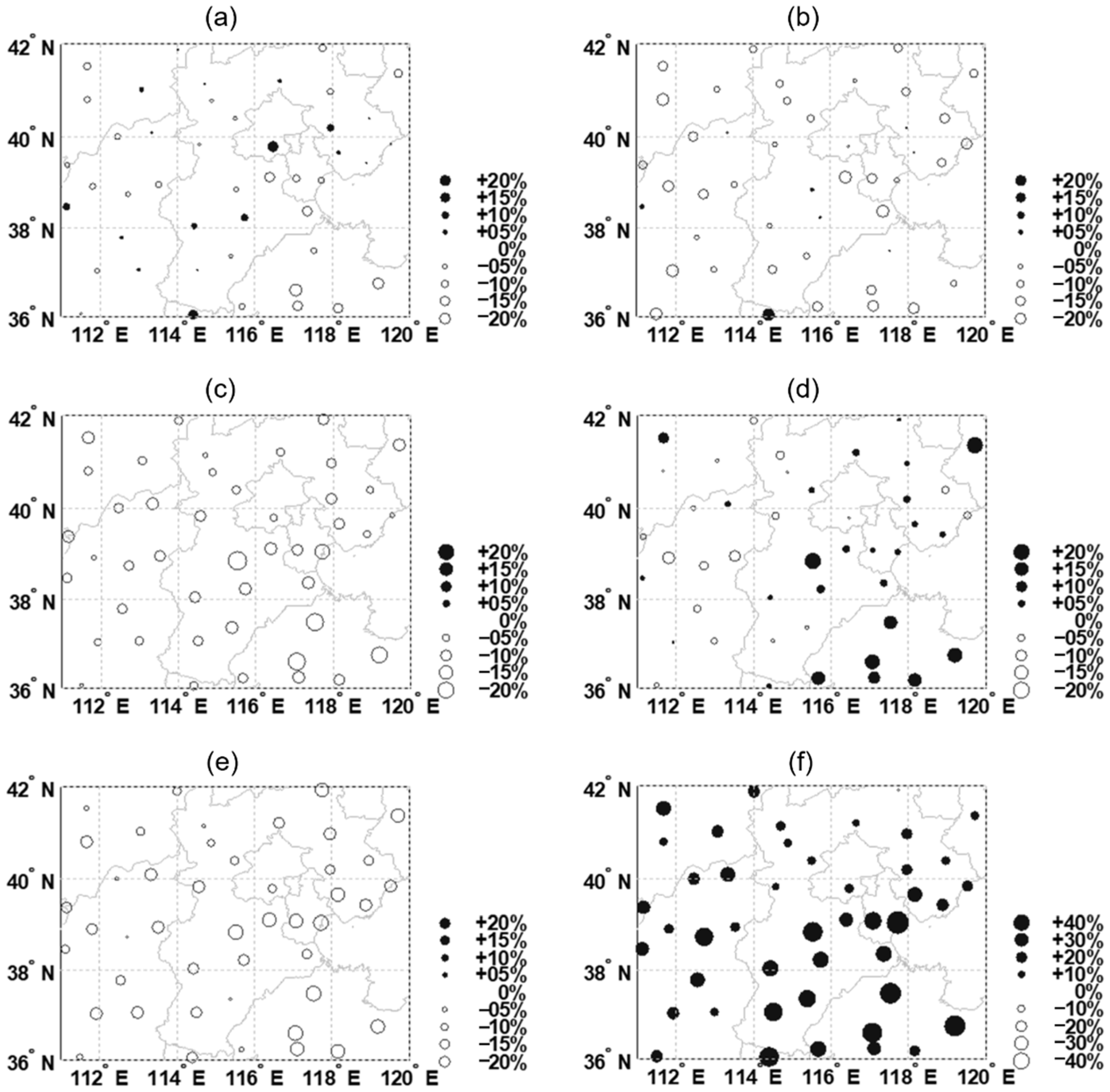
For each station, the downscaled simulation errors have obvious spatial distribution differences. The spatial distribution of the simulation errors is plotted below for each station (Figure 14a–f).
- a. Evaluation of Precipitation Simulations
The observed values of total precipitation (Prtot) in summer and the error percentages of the downscaled results are plotted in Figure 14a. The downscaled simulation errors of each station are positive and negative, with the average size of 25.3 mm and the average error percentage of total precipitation Prtot of each station is −7.4%, which indicates that the SOM-SD model has a strong ability to simulate total precipitation (Prtot).
The spatial distribution of the simulation error and error percentage of the precipitation intensity SDII relative to the station precipitation observations are plotted in Figure 14b. The simulation error is negative at most stations with a mean value of −1.1 mm/day, and the mean SDII error percentage is −11.6%. This indicates that the downscaling model underestimates the precipitation intensity at most stations.
- b. Evaluation of Precipitation Frequency Simulations
In addition to the precipitation amount, another important indicator is precipitation frequency. The frequency characterization of precipitation downscaling results is measured by the number of precipitation days above 0.1 mm (nr001). Figure 14c gives the comparison between the downscaled simulation results and the observed values for the nr001 index.
It is calculated that the simulated error of 3.1 days in the number of rain days above 0.1 mm (nr001) in the downscaled results is underestimated compared to the observed values (error percentage −9.8%) at all stations.
- c. Assessment of Extreme Precipitation
The biggest challenge when downscaling precipitation using global climate models is the reproduction of extreme precipitation events, which often have much larger economic and social impacts than the monthly average precipitation. Therefore, finally, the ability of downscaling models to simulate extreme precipitation events needs to be assessed. Here, two sets of metrics are used: The first set is the extreme precipitation contribution P95T, which represents the percentage of precipitation above the 95th percentile of all precipitation (Figure 14d). The second group is CWD and CDD, where CWD denotes the maximum consecutive days with rain (Figure 14e) and CDD denotes the maximum consecutive days without rain (Figure 14f).
In Figure 14d, the contribution of precipitation above the 95th percentile (P95T) is indicated, which has a simulation error of +3.4% and an error percentage of +6.1%, with a relatively good agreement between the downscaled simulation results and the observed values. It indicates that the SOM-SD model has a strong ability to simulate extreme summer precipitation events in North China.
5. Summary and Conclusions
This paper presents a statistical precipitation downscaling model based on self-organizing mapping, the SOM-SD model, which is applied to the simulation of summer precipitation in North China and its applicability is evaluated and tested. The evaluation work uses total precipitation (Prtot), precipitation intensity (SDII), total number of rainy days (nr001), extreme precipitation contribution (P95T), maximum continuous rainy days (CWD), and maximum continuous rainless days (CDD) to evaluate and analyze the simulation results of summer precipitation at 45 stations in North China in terms of precipitation amount, precipitation frequency, and extreme precipitation. The main conclusions drawn are as follows:
- (a)
- The representative local atmospheric states around the stations that are closely associated with the formation of precipitation can be described jointly by a set of climate element fields combined together. A certain atmospheric state can be automatically identified and successfully captured using the SOM-based circulation mode typing method, and they are automatically classified into different categories (i.e., weather patterns), each of which corresponds to a different precipitation probability distribution characteristic.
- (b)
- There is a very significant positive correlation between the interannual variation of the difference in the frequency of wet and dry nodes and the interannual variation of precipitation. It is not necessary for the model to well simulate the frequency of each climate mode. As long as the trend of the difference in the frequency of the wet and dry nodes can be successfully simulated, the trend of precipitation can be estimated. This can provide a new perspective to determine the credibility of the predicted future climate change results.
- (c)
- The selection of forecast factors is a critical aspect of precipitation downscaling, which directly affects the downscaling results. When downscaling precipitation at different stations, it is necessary to select forecast factors for each station separately. In general, among all of the forecast factors, such as hur850, hus850, ua500, and va500 a significant positive correlation is shown with precipitation at most of the stations. The effect of slp, uas, and vas on precipitation was relatively weak and differed significantly among the stations. In the wet node, the variables that contribute more to precipitation are often at high values and are prone to precipitation formation. Conversely, in the dry node, the variables that are more correlated with precipitation are often at low values and are not prone to precipitation formation.
- (d)
- To test the applicability of this precipitation downscaling model in the North China region, the downscaling results were analyzed and evaluated in three aspects, including precipitation amount, precipitation frequency, and extreme precipitation. All of the tested indicators performed well.
- (1)
- In the simulation of probability density function, the simulation results of its probability density curve are in good agreement with the observed values. The values of the indicators are between 0 and 1.5 × 10⁻⁴, and the values of the indicators are between 0.8 and 1. The precipitation indicators, Prtot and SDII, can obtain better simulation results in summer: The average size of the simulation error of the precipitation downscale total precipitation (Prtot) is −25.3 mm (the average error percentage is −7.4%). The precipitation intensity (SDII) shows negative simulation errors at most of the stations, with an average error size of −1.1 mm (the average error percentage is −11.6%).
- (2)
- In general, the downscaling results are able to reproduce the frequency characteristics of the observed values. The total number of rainy days is underestimated to different degrees at all of the stations. The simulated error of the total number of rainy days (nr001) is −3.1 days, and the SOM-SD model slightly underestimates the total number of rainy days (error percentage −9.8%).
- (3)
- In the simulation of extreme precipitation characteristics, the downscaling model is more capable of simulating extreme summer precipitation events in North China, and the extreme precipitation contribution (P95T) is overestimated with an error of 3.4% (error percentage 6.1%). The maximum continuous rain days (CWD) at each station is underestimated by 1.1 days on average (error percentage −20.0%), and the maximum continuous rain-free days (CDD) is overestimated by 3.5 days on average (error percentage 31.1%).
The SOM-SD model can simulate the probabilistic statistical characteristics of daily precipitation in North China, and the downscaling results are good in terms of precipitation amount, precipitation frequency, and extreme precipitation.
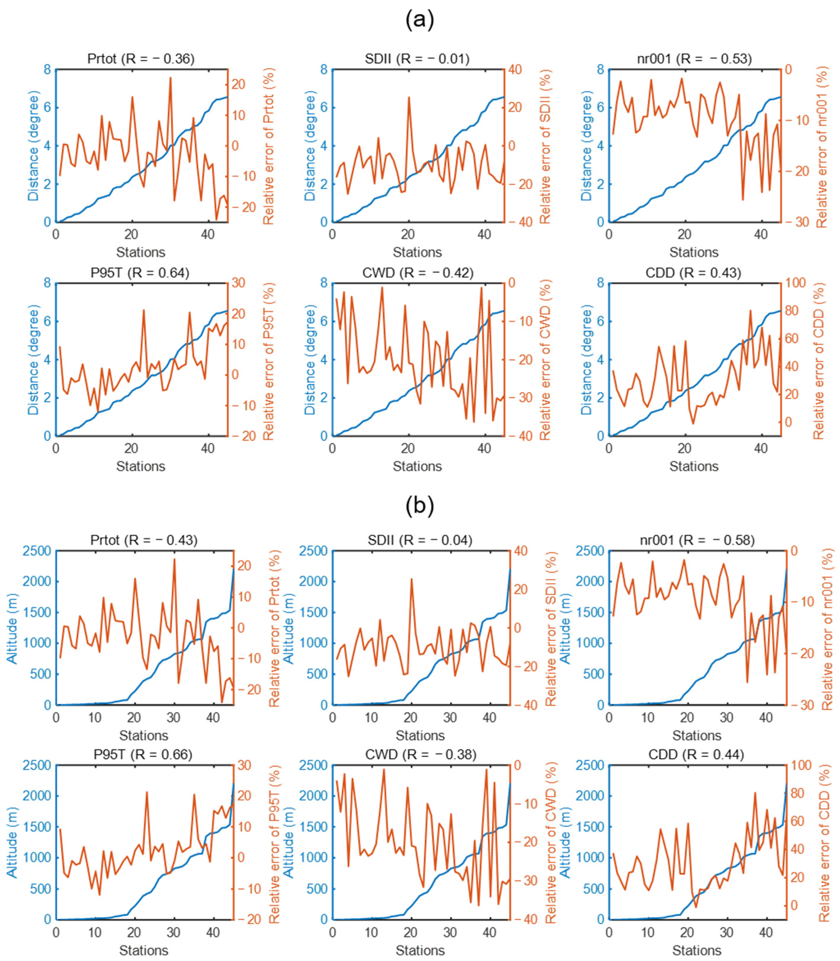
The geographical location of North China is unique in that the summer precipitation in this region is influenced by both the plateau and the ocean. Considering that this influence is very complex and the specific manifestations are different for different stations. Therefore, the last thing that needs to be achieved is to discuss the extent to which there are different levels of simulation accuracy between inland and coastal stations and also stations with different altitudes.
The distance of the station from the coastline was positively correlated with P95T (0.64) and CDD (0.43), negatively correlated with Prtot (−0.36), nr001 (−0.53), and CWD (−0.42), and weakly correlated with SDII (−0.01) (Figure 15a). This result implies an overestimation of precipitation simulations for stations in coastal areas and an underestimation of precipitation simulations for stations located inland.
Altitude was positively correlated with P95T (0.66) and CDD (0.44), negatively correlated with Prtot (−0.43), nr001 (−0.58), and CWD (−0.38), and weakly correlated with SDII (−0.04) (Figure 15b). This result implies an overestimation of precipitation simulations for stations at lower altitudes and an underestimation of precipitation simulations for stations at higher altitudes.
In this paper, the results imply that the different modes obtained using SOM can reflect different characteristics of precipitation distribution. The relationship between weather patterns and precipitation is reasonable. On this basis, the relationship between the main weather modes and the probability distribution of precipitation conditions at each station can be easily established, thus realizing the SOM-SD model. The simulated precipitation has a more consistent daily precipitation probability distribution with the observed precipitation. Moreover, it has some simulation capability for extreme precipitation. The precipitation downscaling method established in this study has good adaptability to North China and can be used for downscaling of current precipitation and scenario prediction of future precipitation in North China. Therefore, this method can significantly improve the downscaling seasonal climate prediction capability of the global climate model for regional precipitation, and can provide an effective means for regional refined seasonal climate prediction.
Author Contributions
Conceptualization, Y.W.; project administration, Y.W.; supervision, X.S.; validation, Y.W.; writing—original draft, X.S.; writing—review and editing, Y.W. All authors have read and agreed to the published version of the manuscript.
Funding
This research was funded by the China Postdoctoral Science Foundation, Grant No. 2018M632334.
Institutional Review Board Statement
Not applicable.
Informed Consent Statement
Not applicable.
Data Availability Statement
The codes and datasets generated during and/or analysed during the current study are available from the corresponding author on reasonable request. The NCEP dataset is available at http://www.cdc.noaa.gov (accessed on 10 August 2019). The NCEP/NCAR 40-Year Reanalysis Project: March, 1996 BAMS National Centers for Environmental Prediction/National Weather Service/NOAA/U.S., Department of Commerce, 1994, updated monthly. NCEP/NCAR Global Reanalysis Products, 1948-continuing. Research Data Archive at NOAA/PSL: /data/gridded/data.ncep.reanalysis.html.
Acknowledgments
This work was supported by the China Postdoctoral Science Foundation (Grant No. 2018M632334). We acknowledge the National Centers for Environmental Prediction (NCEP) for the NCEP reanalysis data (http://www.cdc.noaa.gov, accessed on 10 August 2019). We acknowledge the Meteorological Information Center of China Meteorological Administration for daily precipitation observations (http://cmdp.ncc-cma.net/cn/index.htm, accessed on 10 August 2019). We acknowledge the helpful comments of three anonymous reviewers and the editor, who helped in improving this manuscript.
Conflicts of Interest
The authors declare no conflict of interest. The funders had no role in the design of the study; in the collection, analyses, or interpretation of data; in the writing of the manuscript; or in the decision to publish the results.
References
- Burton, A.; Fowler, H.J.; Blenkinsop, S.; Kilsby, C.G. Downscaling transient climate change using a Neyman–Scott Rectangular Pulses stochastic rainfall model. J. Hydrol. 2010, 381, 18–32. [Google Scholar] [CrossRef]
- Spak, S.; Holloway, T.; Lynn, B.; Goldberg, R. A comparison of statistical and dynamical downscaling for surface temperature in North America. J. Geophys. Res. 2007, 112, D08101. [Google Scholar] [CrossRef] [Green Version]
- Monselesan, D.; Kathleen, L.M. Sea level projections for the Australian region in the 21st century. Geophys. Res. Lett. 2017, 44, 8481–8491. [Google Scholar] [CrossRef] [Green Version]
- Toste, R.; de Freitas Assad, L.P.; Landau, L. Downscaling of the global HadGEM2-ES results to model the future and present-day ocean conditions of the southeastern Brazilian continental shelf. Clim. Dyn. 2018, 51, 143–159. [Google Scholar] [CrossRef]
- Hermans, T.H.J.; Tinker, J.; Palmer, M.D.; Katsman, C.A.; Vermeersen, B.L.A.; Slangen, A.B.A. Improving sea-level projections on the northwestern European shelf using dynamical downscaling. Clim. Dyn. 2020, 54, 1987–2011. [Google Scholar] [CrossRef] [Green Version]
- Shin, S.I.; Alexander, M.A. Dynamical downscaling of future hydrographic changes over the northwest Atlantic Ocean. J. Clim. 2020, 33, 2871–2890. [Google Scholar] [CrossRef]
- Walton, D.B.; Hall, A.; Berg, N.; Schwartz, M.; Sun, F. Incorporating snow albedo feedback into downscaled temperature and snow cover projections for California’s Sierra Nevada. J. Clim. 2017, 30, 1417–1438. [Google Scholar] [CrossRef]
- Lanzante, J.R.; Dixon, K.W.; Nath, M.J.; Whitlock, C.E.; Adams-Smith, D. Some pitfalls in statistical downscaling of future climate. Bull. Amer. Meteor. Soc. 2018, 99, 791–803. [Google Scholar] [CrossRef]
- Linderson, M.; Achberger, C.; Chen, D. Statistical downscaling and scenario construction of precipitation in Scania, southern Sweden. Nord. Hydrol. 2004, 35, 261–278. [Google Scholar] [CrossRef]
- Fowler, H.J.; Kilsby, C.G.; Stunell, J. Modelling the impacts of projected future climate change on water resources in north-west England. Hydrol. Earth Syst. Sci. 2007, 11, 1115–1126. [Google Scholar] [CrossRef] [Green Version]
- Maraun, D.; Rust, H.W.; Osborn, T.J. Synoptic airflow and UK daily precipitation extremes. Extremes 2010, 13, 133–153. [Google Scholar] [CrossRef]
- Maraun, D.; Wetterhall, F.; Ireson, A.M.; Chandler, R.E.; Kendon, E.J.; Widmann, M.; Brienen, S.; Rust, H.W.; Sauter, T.; Themeßl, M.; et al. Precipitation downscaling under climate change: Recent developments to bridge the gap between dynamical models and the end user. Rev. Geophys. 2010, 48, RG3003. [Google Scholar] [CrossRef]
- Wilby, R.L.; Charles, S.P.; Zorita, E.; Timbal, B.; Whetton, P.; Mearns, L.O. Guidelines for use of climate scenarios developed from statistical downscaling methods. Supporting Mater. Intergov. Panel Clim. Change Available DDC IPCC TGCIA 2004, 27, 1–27. [Google Scholar]
- Hewitson, B.C.; Crane, R.G. Self-organizing maps: Applications to synoptic climatology. Clim. Res. 2002, 22, 13–26. [Google Scholar] [CrossRef]
- Hewitson, B.C.; Crane, R.G. Consensus between GCM climate change projections with empirical downscaling: Precipitation downscaling over South Africa. Int. J. Climatol. 2006, 26, 1315–1337. [Google Scholar] [CrossRef]
- Cavazos, T. Large-scale circulation anomalies conducive to extreme precipitation events and derivation of daily rainfall in northeastern Mexico and southeastern Texas. J. Clim. 1999, 12, 1506–1523. [Google Scholar] [CrossRef]
- Chen, L.; Lim, W.; Zhang, P.; Wang, J. Application of a new downscaling model to monthly precipitation forecast. Quarterly J. Appl. Meteorol. 2003, 14, 648–655. [Google Scholar]
- Jia, X.; Chen, L.; Li, W.; Chen, D. Statistical downscaling based on BP-CCA: Predictability and application to the winter temperature and precipitation in China. Acta. Meteorol. Sin. 2010, 68, 398–410. [Google Scholar]
- Wei, F.; Huang, J. A study of downscaling factors of atmospheric circulations in the prediction model of summer precipitation in Eastern China. Chin. J. Atmos. Sci. 2010, 34, 202–212. [Google Scholar]
- Kalnay, E.; Kanamitsu, M.; Kistler, R.; Collins, W.; Deaven, D.; Gandin, L.; Iredell, M.; Saha, S.; White, G.; Woollen, J.; et al. The NCEP/NCAR 40-year reanalysis project. Bull. Amer. Meteor. Soc. 1996, 77, 437–471. [Google Scholar] [CrossRef] [Green Version]
- Xia, J.; Zhang, L.; Liu, C.M.; Yu, J. Towards better water security in North China. Water Resour. Manage. 2007, 21, 233–247. [Google Scholar] [CrossRef]
- Guo, Y.; Li, J.; Li, Y. A Time-Scale Decomposition Approach to Statistically Downscale Summer Rainfall over North China. J. Clim. 2012, 25, 572–591. [Google Scholar] [CrossRef]
- Ruan, C.; Li, J. An improvement in a time-scale decomposition statistical downscaling prediction model for summer rainfall over North China. Chin. J. Atmos. Sci. 2016, 40, 215–226. [Google Scholar]
- Ning, L.; Mann, M.E.; Crane, R.; Wagener, T. Probabilistic projections of climate change for the mid-Atlantic region of the United States: Validation of precipitation downscaling during the historical era. J. Clim. 2012, 25, 509–526. [Google Scholar] [CrossRef] [Green Version]
- Wang, H.; Fan, K. Recent changes in the East Asian monsoon. Chin. J. Atmos. Sci. 2013, 37, 313–318. [Google Scholar]
- Liu, W. Improvements and Implications of Statistical Downscaline Models for Daily Rainfall. Ph.D. Thesis, University of Chinese Academy of Sciences, Beijing, China, 15 March 2013. [Google Scholar]
- Yang, C.; Yan, Z.; Shao, Y. Statistical downscale model for daily precipitation based on Tweedie distribution. J. Beijing Norm. Univ. 2009, 45, 531–536. [Google Scholar]
- Cassano, E.N.; Lynch, A.H.; Cassano, J.J.; Koslow, M.R. Classification of synoptic patterns in the western Arctic associated with extreme events at Barrow, Alaska. Clim. Res. 2006, 30, 83–97. [Google Scholar] [CrossRef] [Green Version]
- Lynch, A.; Uotila, P.; Cassano, J.J. Changes in synoptic weather patterns in the polar regions in the twentieth and twenty-first centuries, part 2: Antarctic. Int. J. Climatol. 2006, 26, 1181–1199. [Google Scholar] [CrossRef]
- Brier, G.W. Verification of forecasts expressed in terms of probability. Mon. Weather. Rev. 1950, 78, 1–3. [Google Scholar] [CrossRef]
- Perkins, S.E.; Pitman, A.J.; Holbrook, N.J.; McAneney, J. Evaluation of the AR4 climate models’ simulated daily maximum temperature, minimum temperature, and precipitation over Australia using probability density functions. J. Clim. 2007, 20, 4356–4376. [Google Scholar] [CrossRef]
- Watterson, I.G. Calculation of probability density functions for temperature and precipitation change under global warming. J. Geophys. Res. 2008, 113, 259–269. [Google Scholar] [CrossRef]
Figure 1.
Study area and station distribution: (a) Topography of the study area (m), (b) distribution of stations.
Figure 1.
Study area and station distribution: (a) Topography of the study area (m), (b) distribution of stations.

Figure 2.
(a) Variable field interpolation (19 hexagons selected around the station). (b) Different methodological procedures applied in this study.
Figure 2.
(a) Variable field interpolation (19 hexagons selected around the station). (b) Different methodological procedures applied in this study.

Figure 3.
Determination of the number of random resampling. As the number of resampling increases, each index value gradually converges with the observed results and gradually stabilizes (repeat sampling has stabilized after 1000 times). The results of different indicators were gradually stabilized: (a) Prtot (mm/season); (b) SDII (mm/day); (c) nr001 (days); (d) P95T (%).

Figure 4.
Forecast factor preference results of the summer precipitation downscaling model for the Beijing station. Except for the three variables (slp, uas, and vas), the other variables have a significant correlation with precipitation.
Figure 4.
Forecast factor preference results of the summer precipitation downscaling model for the Beijing station. Except for the three variables (slp, uas, and vas), the other variables have a significant correlation with precipitation.

Figure 5.
Calculation results of correlation coefficients between forecast factors and precipitation series at various stations in North China.
Figure 5.
Calculation results of correlation coefficients between forecast factors and precipitation series at various stations in North China.

Figure 6.
Cumulative probability distribution function (CDF) of precipitation for the 16 SOM nodes corresponding to the training results.
Figure 6.
Cumulative probability distribution function (CDF) of precipitation for the 16 SOM nodes corresponding to the training results.

Figure 7.
Distribution of 850 hPa relative humidity field (%) for the 16 SOM nodes corresponding to the training results.
Figure 7.
Distribution of 850 hPa relative humidity field (%) for the 16 SOM nodes corresponding to the training results.

Figure 8.
Distribution of vertical decreasing rate of temperature (°C/hm) for the 16 SOM nodes corresponding to the training results.
Figure 8.
Distribution of vertical decreasing rate of temperature (°C/hm) for the 16 SOM nodes corresponding to the training results.

Figure 9.
Distribution of sea level pressure field (hPa) for 16 SOM nodes corresponding to the training results.
Figure 9.
Distribution of sea level pressure field (hPa) for 16 SOM nodes corresponding to the training results.

Figure 10.
Quantitative determination of the indicators of dry and wet nodes. The distribution of node value sizes shows a strong regularity. The value in the upper left corner is generally the largest, and the value in the lower right corner is generally the smallest, with a decreasing trend from the upper left corner to the lower right corner. (a) Number of rainy days (days), (b) total annual precipitation (mm), (c) daily average precipitation (mm/day), (d) 95th percentile precipitation value (mm).

Figure 11.
Comparison of the distribution states of each predictor in the wet and dry nodes at the Beijing station (where the left column figures are the distance level fields of each predictor in the wet nodes and the right column figures are the distance level fields of each predictor in the dry nodes).

Figure 12.
Q-Q plots of summer precipitation (mm day−1) downscaling results (with stations in Beijing, Tianjin, Shijiazhuang, Hohhot, Taiyuan, and Jinan as examples; the horizontal axis is the precipitation observation and the vertical axis is the precipitation downscaling result). (a) Beijing, (b) Tianjin, (c) Shijiazhuang, (d) Hohhot, (e) Taiyuan, and (f) Jinan.

Figure 13.
Quantitative evaluation of the summer precipitation downscaling probability density function pdf simulation results for each station in North China: (a) Histogram of indicators for each station, (b) histogram of indicators for each station.
Figure 13.
Quantitative evaluation of the summer precipitation downscaling probability density function pdf simulation results for each station in North China: (a) Histogram of indicators for each station, (b) histogram of indicators for each station.

Figure 14.
The relative errors of the six indicators were used to assess the effect of the SOM-SD method: (a) Relative error of Prtot (%); (b) relative error of SDII (%); (c) relative error of nr001 (%); (d) relative error of P95T (%); (e) relative error of CWD (%); (f) relative error of CDD (%).
Figure 14.
The relative errors of the six indicators were used to assess the effect of the SOM-SD method: (a) Relative error of Prtot (%); (b) relative error of SDII (%); (c) relative error of nr001 (%); (d) relative error of P95T (%); (e) relative error of CWD (%); (f) relative error of CDD (%).

Figure 15.
Contrast of simulation accuracy between (a) inland and coastal stations (sorted by the shortest distance from the coastline); (b) different altitude stations (sorted by altitude).
Figure 15.
Contrast of simulation accuracy between (a) inland and coastal stations (sorted by the shortest distance from the coastline); (b) different altitude stations (sorted by altitude).


Table 1.
Definition of precipitation index.
| Acronym | Definition | Unit |
|---|---|---|
| Prtot | Total season precipitation | mm/season |
| SDII | Simple daily intensity (mean daily precipitation on wet days) | mm/day |
| nr001 | Mean number of rainy days for daily precipitation ≥0.1 mm | Days |
| P95T | Percentage of rainfall from events beyond 95th percentile value of overall precipitation | Percent |
| CWD | Maximum consecutive wet days | Days |
| CDD | Maximum consecutive dry days | Days |
Table 2.
Comparison of precipitation downscaling results with observed values (observations and simulations were averaged at 45 stations, respectively, and then the errors were calculated).
Table 2.
Comparison of precipitation downscaling results with observed values (observations and simulations were averaged at 45 stations, respectively, and then the errors were calculated).
| Acronym | Unit | Observation | Downscaling | Simulation Error | Error Percentage |
|---|---|---|---|---|---|
| Prtot | mm/season | 300.5 | 287.3 | −13.2 | −4.4% |
| SDII | mm/day | 9.5 | 8.5 | −1.0 | −10.5% |
| nr001 | days | 31.8 | 28.7 | −3.1 | −9.7% |
| P95T | percent | 56.9% | 58.3% | 1.4% | 2.5% |
| CWD | days | 5.1 | 4.1 | −1.0 | −19.6% |
| CDD | days | 11.1 | 14.6 | 3.5 | 31.5% |
Publisher’s Note: MDPI stays neutral with regard to jurisdictional claims in published maps and institutional affiliations. |
© 2022 by the authors. Licensee MDPI, Basel, Switzerland. This article is an open access article distributed under the terms and conditions of the Creative Commons Attribution (CC BY) license (https://creativecommons.org/licenses/by/4.0/).
Share and Cite
MDPI and ACS Style
Wang, Y.; Sun, X. Simulation and Evaluation of Statistical Downscaling of Regional Daily Precipitation over North China Based on Self-Organizing Maps. Atmosphere 2022, 13, 86. https://doi.org/10.3390/atmos13010086
AMA Style
Wang Y, Sun X. Simulation and Evaluation of Statistical Downscaling of Regional Daily Precipitation over North China Based on Self-Organizing Maps. Atmosphere. 2022; 13(1):86. https://doi.org/10.3390/atmos13010086
Chicago/Turabian StyleWang, Yongdi, and Xinyu Sun. 2022. "Simulation and Evaluation of Statistical Downscaling of Regional Daily Precipitation over North China Based on Self-Organizing Maps" Atmosphere 13, no. 1: 86. https://doi.org/10.3390/atmos13010086
Note that from the first issue of 2016, this journal uses article numbers instead of page numbers. See further details here.