Article

The Effect of Atmosphere-Ocean Coupling on the Structure and Intensity of Tropical Cyclone Bejisa in the Southwest Indian Ocean

1
Laboratoire de l’Atmosphère et des Cyclones, CNRS, Université de La Réunion, Météo-France, Saint-Denis, 97400 La Réunion, France
2
Laboratoire d’Aérologie, Université de Toulouse, UT3, CNRS, IRD, 31400 Toulouse, France
3
Institute for Coastal Marine Research (CMR), Nelson Mandela University, Port-Elizabeth 6031, South Africa
*
Author to whom correspondence should be addressed.
Atmosphere 2021, 12(6), 688; https://doi.org/10.3390/atmos12060688
Submission received: 29 April 2021 / Revised: 20 May 2021 / Accepted: 21 May 2021 / Published: 27 May 2021
(This article belongs to the Special Issue Tropical Cyclones in the Indian Ocean)

Abstract

:
A set of numerical simulations is relied upon to evaluate the impact of air-sea interactions on the behaviour of tropical cyclone (TC) Bejisa (2014), using various configurations of the coupled ocean-atmosphere numerical system Meso-NH-NEMO. Uncoupled (SST constant) as well as 1D (use of a 1D ocean mixed layer) and 3D (full 3D ocean) coupled experiments are conducted to evaluate the impact of the oceanic response and dynamic processes, with emphasis on the simulated structure and intensity of TC Bejisa. Although the three experiments are shown to properly capture the track of the tropical cyclone, the intensity and the spatial distribution of the sea surface cooling show strong differences from one coupled experiment to another. In the 1D experiment, sea surface cooling (∼1 °C) is reduced by a factor 2 with respect to observations and appears restricted to the depth of the ocean mixed layer. Cooling is maximized along the right-hand side of the TC track, in apparent disagreement with satellite-derived sea surface temperature observations. In the 3D experiment, surface cooling of up to 2.5 °C is simulated along the left hand side of the TC track, which shows more consistency with observations both in terms of intensity and spatial structure. In-depth cooling is also shown to extend to a much deeper depth, with a secondary maximum of nearly 1.5 °C simulated near 250 m. With respect to the uncoupled experiment, heat fluxes are reduced from about 20% in both 1D and 3D coupling configurations. The tropical cyclone intensity in terms of occurrence of 10-m TC wind is globally reduced in both cases by about 10%. 3D-coupling tends to asymmetrize winds aloft with little impact on intensity but rather a modification of the secondary circulation, resulting in a slight change in structure.

1. Introduction

According to World Meteorological Organization’s Ninth International Workshop on Tropical Cyclones (IWTC-9, 2018), the recent deployment of new high space-time resolution geostationary and low-earth orbiting satellites over open oceans, together with ongoing improvements in numerical weather prediction (NWP) models have substantially improved the prediction of tropical cyclone (TC) tracks in all TC basins [1,2]. Predictions of TC intensity, on the other hand, have proven to be more complicated and have been shown to improve significantly more slowly over the last few years. Although sources of progress in TC intensity forecast are numerous, it is generally accepted that the most effective way for improving TC forecast in both NWP e.g., [3] and climate e.g., [4] models consist in coupling atmosphere and ocean models to more effectively represent the multi-scale response and feedback of the upper ocean on boundary layer processes. Indeed, the energy required for genesis, sustenance and intensification of a TC primarily originates from the ocean through sea surface temperature (SST) and air-sea fluxes of heat and moisture e.g., [5]. These interactions have also recently been shown to play a key role in the cold wake properties at the sea surface, which can not only impact the intensity of the cyclone itself, but also influence the structure of the ocean-atmosphere coupled system for up to several weeks [6].
TCs interact with the SST in three ways [7]: the heat transport to the atmosphere e.g., [8], the vertical mixing with deeper water e.g., [9], and the upwelling generated by Ekman pumping e.g., [10]. While the first (resp. second) process could be easily represented by using a slab ocean model (resp. a 1D mixed-layer model), a three-dimensional model is nonetheless required to properly represent all three processes.
In uncoupled TC simulations, the feedback from the heat exchange at the surface is not taken into account, allowing for the TC to benefit from an infinite source of energy from the ocean for its intensification. Using a coupled model thus introduces a negative feedback between the TC and the SST, which generally allows mitigating the over intensification of TC in numerical models. The strength of these feedback nevertheless depends on many factors such as ocean stratification e.g., [7] and storm translation speed [11]. The temperature and thickness of the warm layer, which can be defined for TCs as the layer where the ocean temperature exceeds 26 °C, is for instance an important factor governing this feedback [12,13,14]. Moreover, the response of TC to changes in ocean thermal structure is gradual and suggests that changes in storm intensity are highly dependent on the horizontal scale of ocean features along the storm track [15,16]. A realistic representation of air-sea interactions is also essential in the case of slow-moving systems [11,17,18,19]. Because 1D ocean models are not able to reproduce upwelling resulting from the outward horizontal transport of warm waters near the TC core, 3D models seem better suited to represent ocean-atmosphere interactions in the vicinity of TCs. Yablonsky and Ginis [11] showed that 3D ocean coupling was, in particular, essential to capture SST cooling associated with TC translating at less than 5 m s 1 , and even more critical for slower moving systems.
Air–sea coupling can also have a positive feedback on TC intensification through modifying the structure of the boundary layer. Using coupled simulations of Typhoon Choi-Wan (2009), Lee and Chen [20] found that a stable boundary layer (SBL) could form over the cold wake region of the storm in response to the presence of warm air over cooler SST. Through staying longer in the boundary layer, the air enclosed in the SBL—the latter was not present in the uncoupled simulation of the storm—was found to gain additional energy from surface heat and moisture fluxes before being transported into the eyewall region. As a result, the negative effect from the SST cooling was partly offset by the ingestion of this more energetic air into the TC core, which did not only acted to increase the storm efficiency but also to modify its structure.
Previous studies have shown that coupling the atmosphere to the ocean is essential to represent more comprehensively the various feedbacks between a TC and its principal source of energy. Nevertheless, atmosphere-ocean coupling could sometimes have very little impact on the prediction of TC evolution [7]. Because of the substantial resources required to operate a fully 3D ocean model in an operational framework, the choice of implementing 1D or 3D ocean dynamics in operational NWP systems is still an open question in many forecasting centers [3]. So far, these issues have been mostly investigated in an idealized framework and on a limited number of cases.
The objective of this study, conducted as part of the ReNovRisk-Cyclone research programme [21] is to further evaluate the benefit of 1D vs. 3D ocean coupling for tropical cyclone modeling. It is based on numerical simulations of tropical cyclone Bejisa, which passed nearby Reunion Island in January 2014 and has been one of the main research focus of ReNovRisk-Cyclone [22,23]. To achieve this objective, we use a high resolution numerical modeling system based on the coupling of the atmospheric model Meso-NH [24] and a regional configuration of the ocean model NEMO [25]. Various configurations of this modeling system (uncoupled, 1D, 3D) are used to evaluate the impact of ocean coupling on the simulated trajectory, intensity and rainfall production as well as heat and momentum fluxes. This paper is organized as follows. Section 2 provides an overview of the coupled Meso-NH-NEMO modeling system and numerical simulations performed in this study along with a short description of TC Bejisa. Simulation outputs are discussed in Section 3 to assess the simulated TC track and intensity as well as the impact of 1D and 3D air-sea coupling on the ocean and the atmosphere. Conclusions and perspectives are given in Section 4.

2. Models and Experiment Design

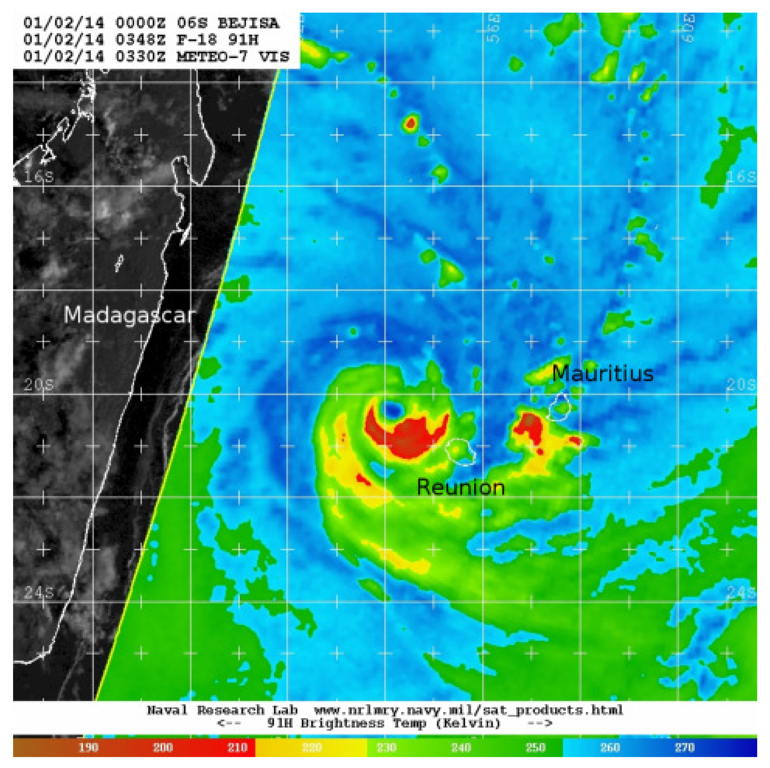
2.1. Case Study: Tropical Cyclone Bejisa

In this section, we recall some key features of tropical cyclone TC Bejisa, which detailed description can be found in Pianezze et al. [26]. TC Bejisa is representative of the storms that regularly affect Reunion Island and has been chosen for its relatively common meridian track, average intensity and speed of displacement [27]. In this study we focus on the period between 1 January 00 UTC and 2 January 12 UTC, which corresponds to the period it passed to the closest to Reunion Island.
On 1 January, the storm was located about 500 km north-northwest of Reunion Island and was moving southwards at an average speed of about 4.7 m s 1 with maximum winds around 40 m s 1 . Over the next 24 h, TC Bejisa accelerated under the influence of an average ridge to the east. On 2 January, a persistent weakness on the north-northeast side of the eyewall could be noticed in Reunion Island’s radar reflectivity field (not shown), suggesting that the TC was about to collapse. Bejisa’s eye passed 50 km from the west coast of the island (Figure 1). After crossing Reunion Island, the TC eye wall was torn off in its north-northwestern part, due to strong northwest winds at high altitude.

2.2. Atmosphere-Ocean Coupled System and Numerical Experiments

The coupled system used in this study is based on the atmospheric model Meso-NH [24] and the ocean model Nucleus for European Modeling of the Ocean (NEMO [25,28]).
Meso-NH is the non-hydrostatic mesoscale atmospheric model of the French scientific community (http://mesonh.aero.obs-mip.fr accessed on 21 May 2021). For this study, Meso-NH has been configured on a domain of 1500 km by 1000 km around Reunion Island, as shown in Figure 2. The horizontal grid resolution was set to 2 km with 70 stretched vertical levels, including 20 levels below 2 km altitude. The microphysics scheme is a one moment bulk mixed-phase scheme that predict five hydrometeor species: cloud water, rain, cloud ice, snow and graupel [29]. The shallow convection is taken into account using mass-flux calculations [30]. The turbulence scheme, based on 1.5-order closure scheme [31], is used in its 1D version with the mixing length of Bougeault and Lacarrere [32]. The radiation scheme is the one used at ECMWF [33]. The bulk iterative Exchange Coefficients from Unified Multi-campaigns Estimates (ECUME) sea surface turbulent fluxes parameterization [34] is used over the ocean and is coupled with the SURFEX surface model to represent atmospheric interactions with the Earth’s surface [35].
NEMO (https://www.nemo-ocean.eu/ accessed on 21 May 2021) is a primitive equation ocean model. This study uses the ocean component of version 3.6 of the code. NEMO is used in a regional configuration that covers the same region as the atmospheric model (Figure 2). The horizontal resolution is set to 1/12° (about 9 km in this region). On the vertical, 50 unevenly spaced levels are used as in the 1/12° resolution PSY4V2 global operational model [36]. Bathymetry is based on the ETOPO1 database [37]. The vertical mixing is a turbulent kinetic energy closure scheme based on Gaspar et al. [38] (like the 1D oceanic mixing layer used in this study), but with significant modifications introduced by Madec et al. [39] in the implementation and formulation of the mixing length scale. The split-explicit free surface formulation of Shchepetkin and McWilliams [40] is used.
The ocean-atmosphere interface is based on SURFEX and the OASIS3-MCT coupler [41]—a full description of the interface and coupling strategy is detailed in Voldoire et al. [42].
A set of 3 simulations was carried out from the same initial state, but with differences in the treatment of the coupling between the atmosphere and the ocean: NOCPL (no coupling i.e., SST constant), OML1D (1D ocean mixed layer) and CPL3D (full 3D ocean). The characteristics of these simulations are summarized in Table 1. The initial conditions for the atmosphere are taken from the 2.5 km resolution research version of the AROME-IO model [3], which is equipped with a 3DVAR assimilation system and is coupled to a 1D oceanic mixing layer model. Both AROME-IO and Meso-NH share the same physical parameterizations but use a different advection scheme. The lateral boundary conditions are derived from the ECMWF analyses at 16 km horizontal resolution every 6 h.
Mercator-Ocean PSY4V2 analysis and forecasts are used to initialize and force the ocean model. In uncoupled simulations, the usual procedure is to initialize the ocean surface from ECMWF ocean fields. In our case, Mercator PSY4V2 analysis is nevertheless used to initialize the NOCPL simulation to make sure that the initial SST conditions are the same for all simulations (Figure 2a) and get rid of the impact of the ocean initial state on the simulations. In the NOCPL experiment, the SST remains constant throughout the simulation. In the OML1D experiment, the SST evolves by activating the 1D oceanic mixing layer model which is part of the SURFEX model [43]. The latest simulation, CPL3D, includes the fully coupled system in which the atmosphere and ocean exchange information every hour. The ocean sends SST and currents to the atmosphere, while the atmosphere sends heat and momentum fluxes as well as precipitation to the ocean.
It is also important to note that the atmospheric spin-up is almost totally mitigated as the high-resolution AROME-IO analysis used to initialize the simulations has almost the same resolution as Meso-NH (2.5 km against 2 km, respectively). In the ocean, there is no spin-up either, as the resolution of the NEMO-PSY4 analysis is identical to that of the regional configuration of NEMO used in this study.
All simulations are initialized at 00 UTC on 1 January 2014 and run over 36 h, i.e., the period when the TC approaches and passes to the closest to Reunion Island.
The computational costs of these simulations are detailed in Table 1. The atmospheric and oceanic models use 600 and 12 processors, respectively. Since the oceanic mixed layer model is included in the surface scheme of Meso-NH, no additional processors are required for it. The additional cost of 78 h (+∼1% wrt NOCPL cost) in the OML1D experiment corresponds to the computational cost of the OML scheme. The additional cost of 47 h (+∼0.6% wrt NOCPL) in the CPL3D experiment is mostly due to the exchange of fields between the atmosphere and the ocean as NEMO runs much faster than Meso-NH in this configuration.
Figure 2a shows the SST field at initialization time along with the buoy data available at that time. Colored circles indicate observed SST value. Temperatures warmer than 26 °C are seen over almost all the domain, with maximum values of about 29 °C around 20° S. The colder temperatures observed in the northern part of the domain are indicative of the cold wake generated by TC Bejisa in Mercator-Ocean analysis. This initial SST field shows good agreement with buoy observations (black circles). At initialization time, the ocean mixed layer (OML) near Reunion Island extends within the first 40 m with an average temperature of 28.5 °C. Underneath the OML, the temperature progressively drops to reach 26 °C at 60 m depth and then drops again faster to attain 23 °C at 150 m depth (Figure 2c). The vertical temperature profile is quite uniform over the area impacted by TC Bejisa with slightly colder temperature southward of the TC but with similar profiles. The MSLP simulated after 12 h in the CPL3D simulation (Figure 2b) also shows good agreement with buoy observations collected in the vicinity and far range of the TC.

3. Results

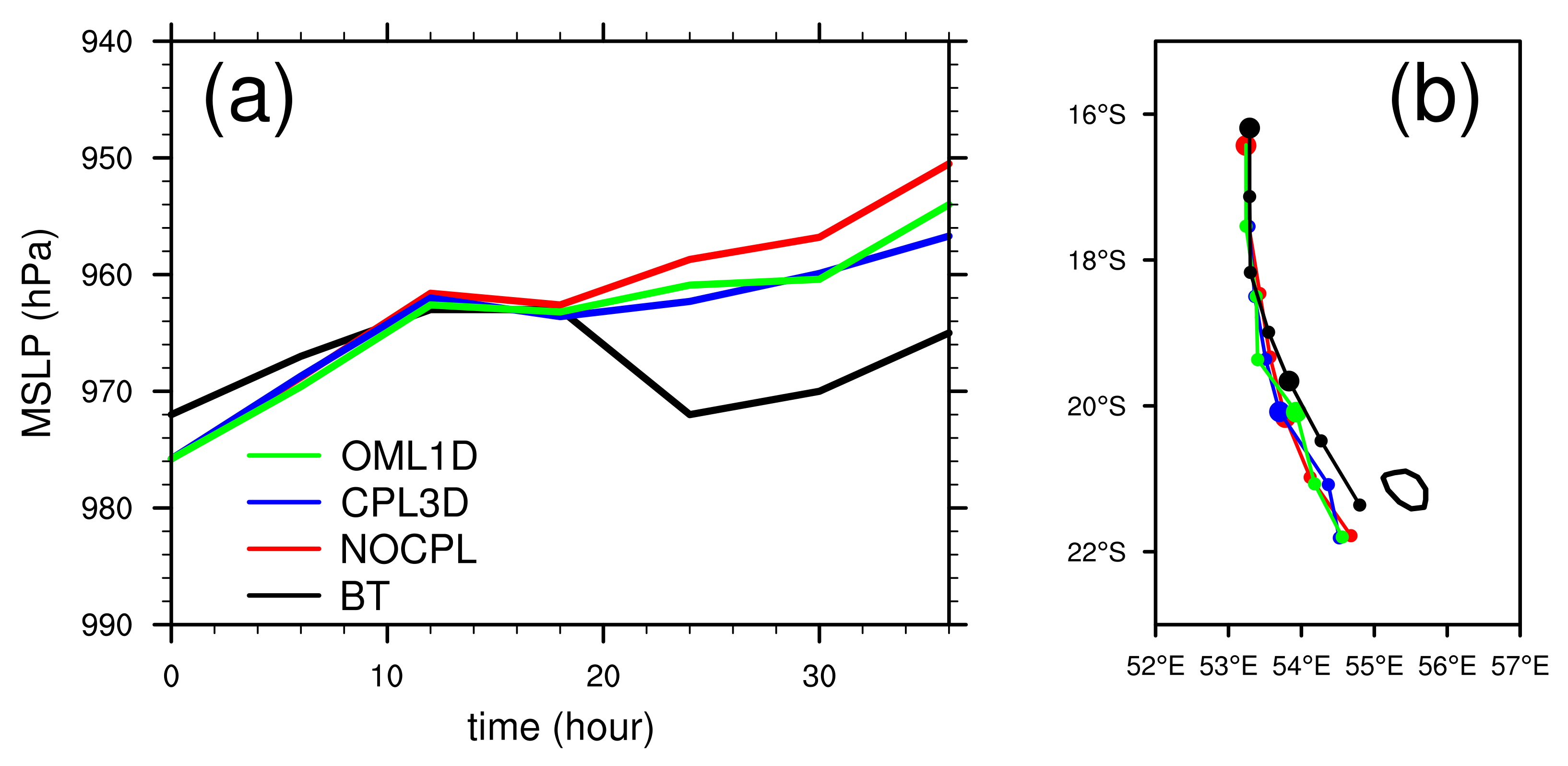
3.1. Track and Intensity
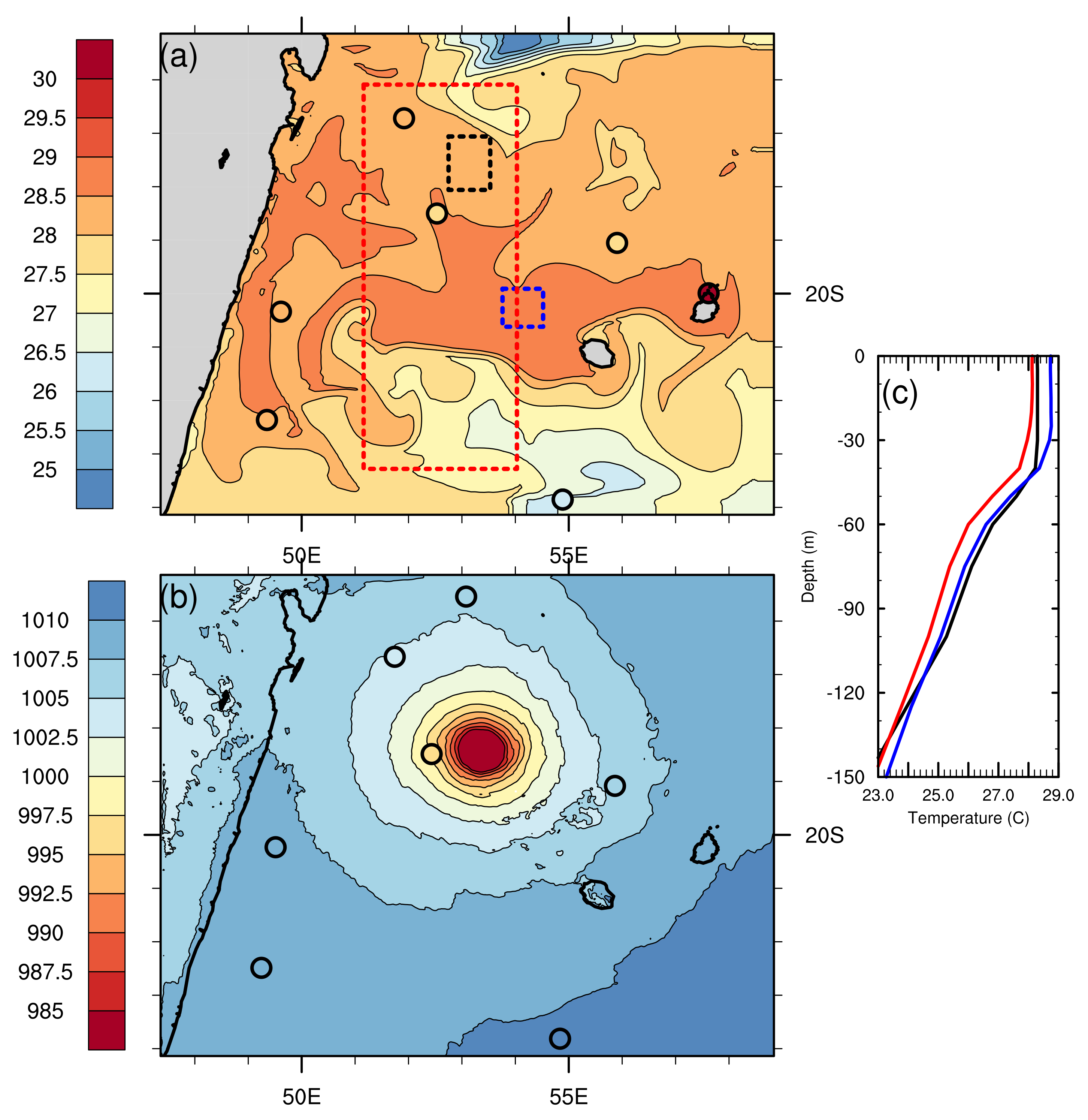
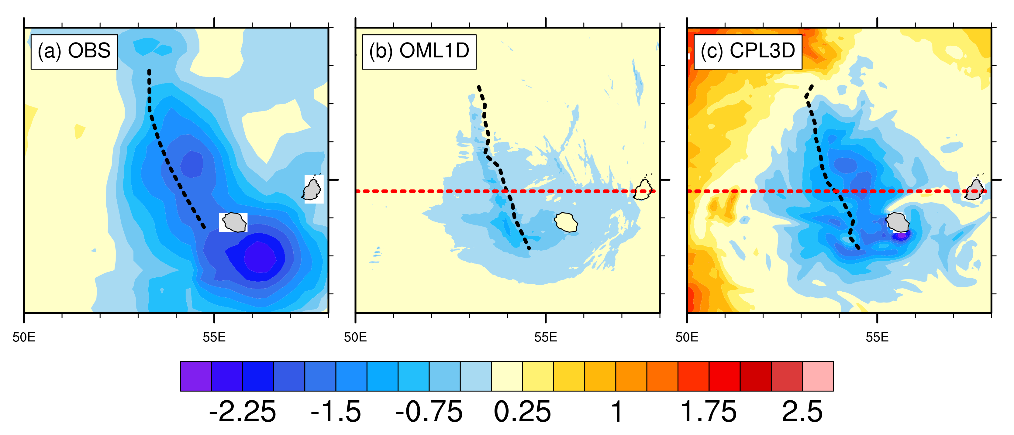
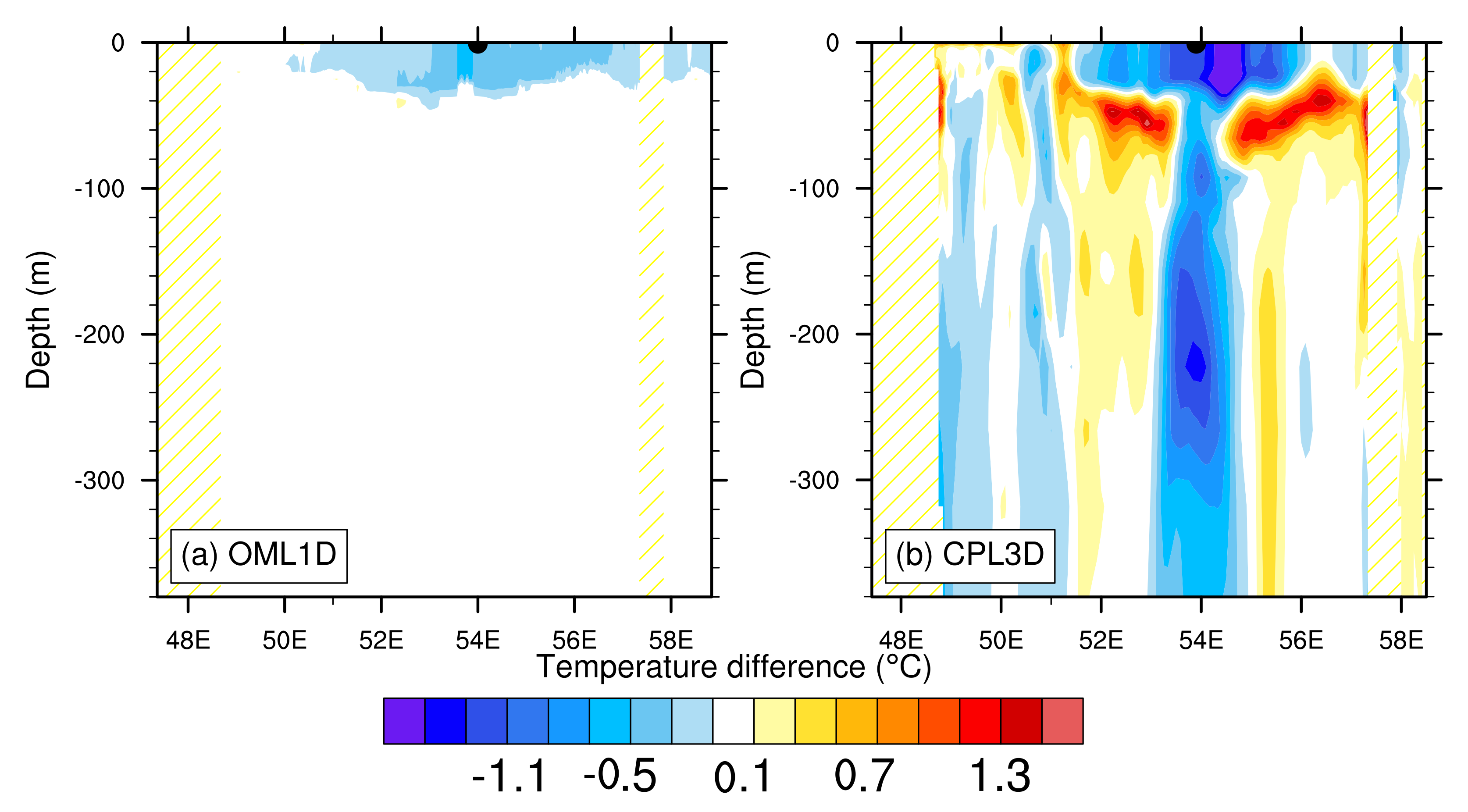
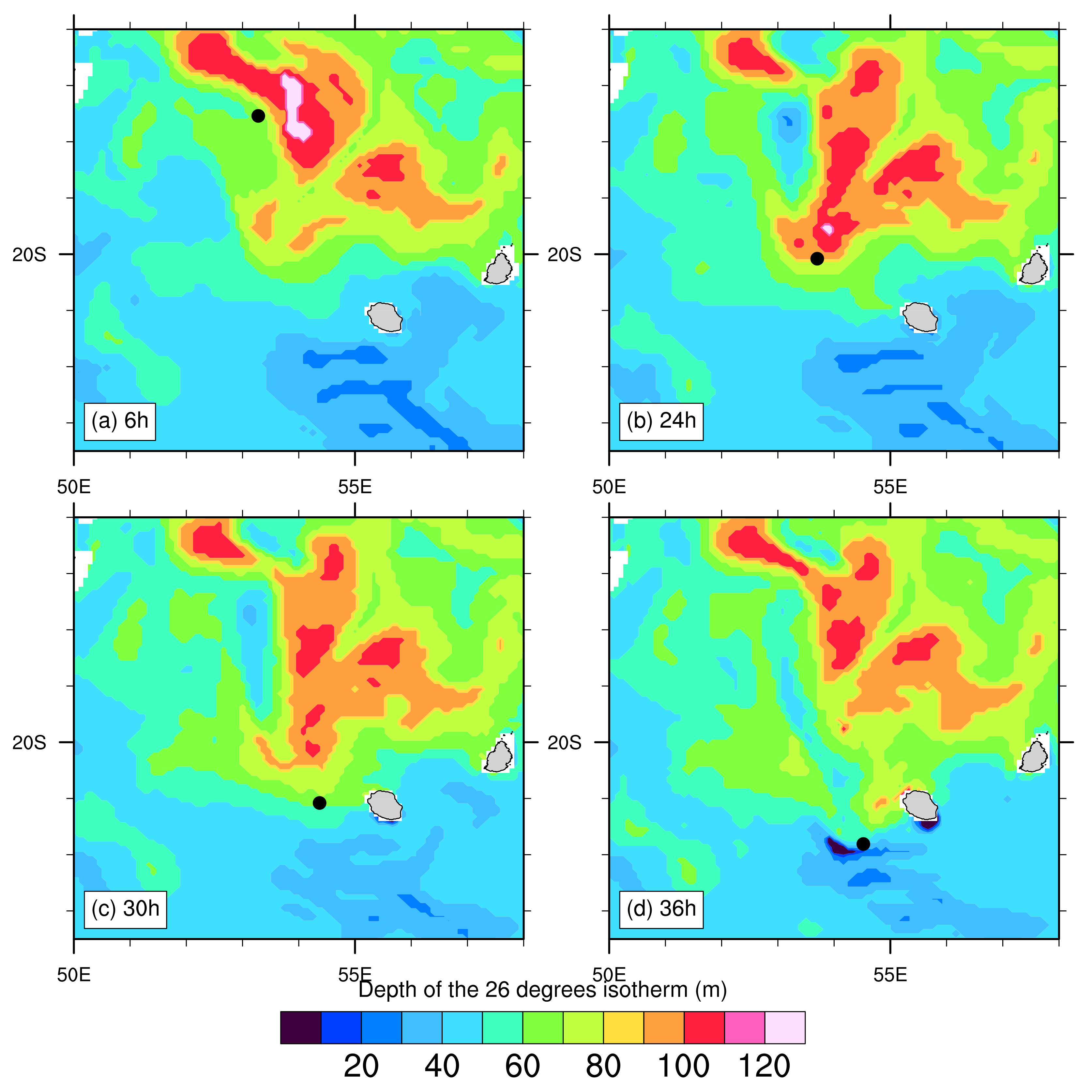
TC tracks simulated in the three experiments (Figure 3a) are relatively similar and are close to the best-track estimate analyzed by the regional specialized meteorologicval center (RSMC) La Réunion (black line), despite a slight westward error in TC position. The error in position is approximately 50 km after 36 h of simulations with a mean error of 45 km for all times. As expected e.g., [26], the coupling and the degree of coupling do not modify significantly the modelled tracks.
The simulated translation speeds are between 4 and 7 m s 1 , also in good agreement with RSMC La Réunion analysis (not shown). The mean (standard deviation) 36-h translation speed in the NOCPL, OML1D and CPL3D simulations is 5.35 m s 1 (0.89), 4.3 m s 1 (0.91) and 5.8 m s 1 (1.45), respectively. TC Bejisa thus tends to move slightly slower (resp. faster) in the OML1D (resp. CPL3D) experiment than in the NOCPL simulation, with slightly larger variations for the CPL3D experiment. The translation speed is a crucial parameter for controlling the underlying ocean response and the subsequent SST cooling feedback to the storm. A translation speed of 5 m s 1 seems to be a threshold below which the differences in cooling between a 1D and a 3D ocean model are greater compared to the differences with a faster translation speed [11,16]. The translation speed of TC Bejisa is close to this threshold value, which could limit the effect of the degree of coupling on the ocean cooling.
The simulated intensity (MSLP, Figure 3b) matches best-track data very well during the first 18 h of simulation. Despite a slight intensity deficit (∼4 hPa) at initialization time, the three simulations are able to capture the first intensification of the TC (up to 962 hPa), and the following plateau. Between 18 and 24 h, none of them is nevertheless able to capture the storm weakening analyzed in the best-track (−9 hPa in 6 h). After 24 h, best-track data also show a re-intensification of the system (7 hPa in 12h), which is well reproduced in the 3 simulations. After 18 h, the uncoupled and coupled experiments start to diverge. Simulation NOCPL shows the highest intensity with MSLP values 7 hPa (resp. 4 hPa) higher than in the CPL3D (resp. OML1D) experiment at the end of the simulation.

3.2. Oceanic Impact

Figure 4 shows the SST difference between observations (Figure 4a) and the OML1D (Figure 4b) and CPL3D (Figure 4c) simulations over the 30-h period 1 January, 06 UTC-2 January, 12 UTC. Observations are derived from daily high-resolution (0.25° × 0.25°) analyses (combination of Ship, Buoy, AVHRR: NOAA19, METOP, NCEP-ice data https://www.ncdc.noaa.gov/oisst/optimum-interpolation-sea-surface-temperature-oisst-v20 accessed on 25 April 2016). Two cooling maxima can be seen in the observations; a first one (of nearly 1.5 °C) north of Reunion island (to the left hand side of the TC track), and a second one (of nearly 2 °C) south of Reunion island. The values of SST cooling induced by the TC in the CPL3D simulation (Figure 4c) agrees well with observations (Figure 4a) in terms of intensity and location. The simulated maximum cooling area to the left of the TC track occurs in a region of maximum surface current with values around 1.5 m s 1 (not shown). This result is consistent with previous studies showing that the largest SST cooling is generally found to the right hand side of TC tracks in the Northern Hemisphere [17,44,45,46,47], and to their left hand side in the Southern Hemisphere [48]. This rightward/leftward bias is due to the TC wind-stress vector, which turns clockwise (resp. anti-clockwise) with time on the right (resp. left) hand side of the TC track to the north (resp. south) of the equator. As it is roughly resonant with the mixed layer velocity, this causes strong entrainment and thus enhanced SST response. The cooling pattern of TC Bejisa in both CPL3D and satellite observations is 3 to 4 times weaker on the left side of the system, which is again consistent with previous studies [17]. South of Reunion Island, the cooling simulated in the CPL3D experiment is also roughly comparable to that deduced from composite observations.
In experiment OML1D (Figure 4a), the SST cooling is reduced by a factor of 2 compared to CPL3D due to the lack of upwelling resulting from the absence of horizontal transport in the 1D ocean model. Moreover the maximum cooling in experiment OML1D is located on the right hand side on the TC track, contrary to both CPL3D and observations.
Yablonsky and Ginis [11] showed that the missed part of SST cooling in 1D ocean models depends partly on the properties of the OML depth in the initial upper-ocean profile. They showed that the deeper the OML is, the slower the TC translation speed is required to make a difference between 1D and 3D coupling. In our case, the structure of the OML under TC Bejisa shows a warmer surface temperature and a depth of the 26 °C isotherm at 75 m, i.e., in between the 2 profiles used in the former idealized study. Zhao and Chan [49] found that the optimal speed for TC development when the mixed layer depth is thick enough (at least 50 m) is 3 m s 1 . A TC with similar translation speed and intensity thus causes weaker SST cooling with a thicker warm upper layer than it does with a shallower OML [50,51].
The corresponding vertical structure of the temperature anomaly (west-east cross section) is shown in Figure 5 for the NOCPL (Figure 5a) and CPL3D (Figure 5b) experiments. The CPL3D experiment shows two interconnected regions with strong cooling. The primary maximum is located on the left side of the track between the surface and 40 m depth and exceeds 1.5 °C. At the surface, the cooling extends horizontally over 200 km on both sides of the trajectory and is maximum within the first 80 km from the storm center on the left side. The second region of cooling is located just underneath the first one. Its horizontal extension is ∼2.5 less than the primary one, but it extends vertically well below 300 m depth. In this area, the maximum cooling reaches 1.3 °C at 220 m depth and is located right below the TC center. Strong heating (>1.3 °C) is observed on both sides of the upwelling between the bottom of the mixing layer and 80 m depth. This result agrees well with previous studies e.g., [52] that show a cooling within the initial OML (due primarily to entrainment), a warming just below the initial position of the OML depth resulting from entrainment, and a cooling mainly due to upwelling underneath. In particular, Lin et al. [52] showed that the contribution of upwelling to the temperature anomaly within 75 km of a typhoon track is smaller in the surface layer but larger below, with upwelling contributing to ocean cooling by 15% up to 30 m depth, 84% between 30 and 250 m and 94% between 250 et 600 m.
In the OML1D experiment, only one region of cooling that does not exceed 0.7 °C can be observed. This area is also confined within the OML (Figure 5a).
Although SST plays an important role in the genesis of TC, it has been shown that the heat content of the ocean between the sea surface and the depth of the 26 °C isotherm (D26), also called tropical cyclone heat potential (TCHP), plays an important role in TC intensity changes [14]. TCHP is defined as a measure of the integrated vertical sea temperature from the surface to D26 [53]. Figure 6 shows the spatial variation of D26 in the CPL3D simulation. After 6 h of simulation (Figure 6a), D26 is located between 60 and 80 m, in the immediate vicinity of the TC center. D26 is also quite deep (∼90–100 m in Figure 6a–c) to the rear of the modelled TC. The low values (∼30–40 m) of D26 associated with the cooling of the ocean by the cyclone are observed 200 to 300 km behind the TC center. It is also worth noting that strong values of D26 between 18 and 20° S can only be seen after 24 h of simulation.
In the OML1D simulation there is almost no evolution of D26 throughout the 36 h of simulation. Such behaviour is not surprising as cooling is twice as low as in the CPL3D experiment and is confined to the 50 upper meters of the ocean.

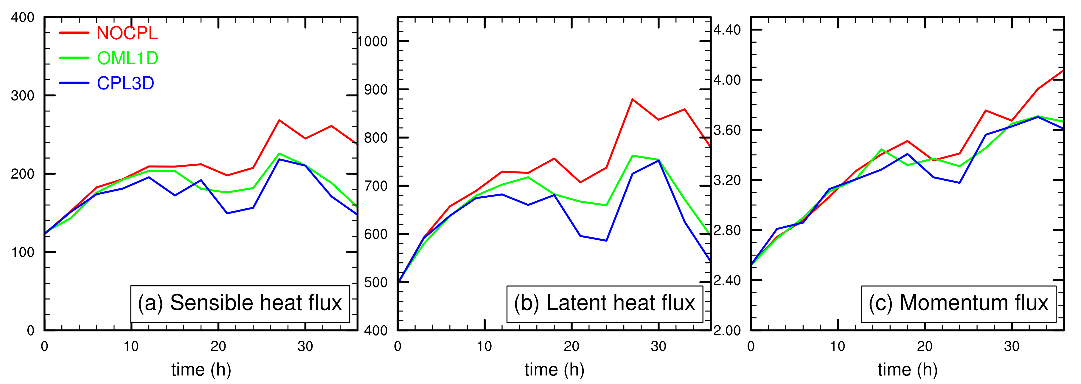
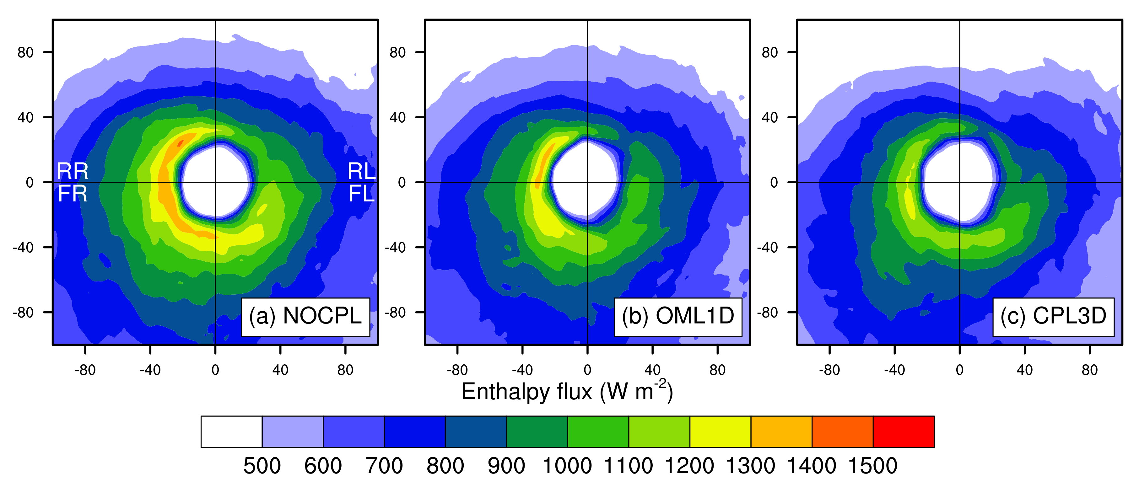
3.3. Atmospheric Impact

In this section, we investigate the impact of ocean-atmosphere coupling on the atmospheric part of the system, starting from the interface and going upwards. The primary objective is to determine if structural changes occur in the atmosphere with the degree of ocean coupling.
To assess the impact of the degree of coupling on the surface fluxes, fluxes at the interface (sensible and latent heat flux, and momentum flux) are averaged every 3 h over a region of 100 km × 100 km centered around the eye of the system. Figure 7 shows the temporal evolution of these mean fluxes. Significative differences in mean heat flux between the 3 experiments appear after 6 h of simulation. The maximum heat fluxes are found on 2 January at 03 UTC (after 27 h of simulation) in the 3 simulations.
A reduction of about 20% of the heat fluxes in the inner core region of the TC is observed in both coupled simulations compared to the NOCPL experiment. The flux differences between the OML1D and CPL3D experiments are small, even though heat fluxes in CPL3D tend to be slightly weaker overall. The differences appear slightly later for the momentum flux (after 10h of simulation) and are less significant (Figure 7c). However, the overall trend is similar to that for heat fluxes, with the NOCPL experiment producing higher turbulent fluxes than the ocean-atmosphere coupled simulations.
Each averaging box has been decomposed into four areas (i.e., by square of 50 km × 50 km): rear left (RL), rear right (RR), front left (FL) and front right (FR) (cf Figure 8, top left panel) with respect to TC displacement to emphasize the asymmetric response of ocean-atmosphere coupling on air-sea fluxes. Figure 8 shows the enthalpy flux (latent + sensible heat fluxes) composited over the whole simulation for the 3 simulations.
The coupling with the ocean and the storm-induced SST cooling produces a weaker storm with reduced surface enthalpy flux from the ocean. The strongest differences arise from the rear part of the TC and more particularly from the rear left quadrant. This enhances the asymmetry with relatively lower values in the rear-right quadrant of the storm due to the presence of a persistent cold wake. The main difference are thus located both to the front, and to the rear of the TC where strong reduction of enthalpy fluxes occurs.
Figure 9 shows the normalized (with respect to the NOCPL simulation) probability density function (PDF) of the 10-m wind for five storm intensity classes according to TC classification used in the SWIO: tropical depression (TD, 14–17 m s 1 ), moderate tropical storm (MTS, 18–24 m s 1 ), severe tropical storm (STS, 25–32 m s 1 ), tropical cyclone (TC, 33–46 m s 1 ), and intense tropical cyclone (ITC, 47–60 m s 1 ). The PDF, computed over the whole simulation domain and from all output times (every 3 h), show that coupling tends to reduce areas of strong winds, with a reduction of 7 to 10% for the TC class and up to 57% for the ITC class. This indicate that ocean-atmosphere coupling predominantly affects highest intensity systems, which usually causes the strongest environmental impacts. The results of the OML1D and CPL3D experiments are generally quite similar even though CPL3D shows fewer regions with ITC winds and slightly more with TC winds.
Figure 10 shows vertical cross sections of mean azimuthal tangential wind, radial wind and vertical velocity composites averaged over the entire simulation (to mitigate errors due to slightly different timing and position of the TC), using hourly model outputs over a radius of 100 km from the TC center. Note that azimutally averaged fields tend to misrepresent the overall TC inflow structure, especially the asymmetric one [54]. The main difference between the three simulations concerns the maximum intensity of the tangential wind, which shows weaker wind values when the atmosphere is coupled to the ocean (in line with the overall reduction of surface fluxes). The secondary circulation shows more difference between the 3 simulations than for the primary one, with a less intense secondary circulation in OML1D compared to the 2 other experiments. The mean vertical velocity exceeds 1.5 m s 1 between 3 and 7 km altitude in the NOCPL experiment, while values above 1.5 m s 1 are confined in the range 4–6 km altitude in CPL3D. In the OML1D experiment, the mean vertical velocity barely reaches 1.2 m s 1 between 5 and 6 km altitude. A slight shift in the position of the radial and vertical maximum speeds is also noticed, which could indicate a slight change in the size and structure of the TC due to coupling.
The mean structure of the water vapor field over the whole simulation (Figure 11) is quite similar for all three simulations with maximum value observed to the front of the system and the presence of a moist band extending to the rear left side of the TC (with respect to storm motion). The main difference comes from the maximum mean value and spatial extension of the moisture field, which is weaker with the degree of coupling. The simulated TC is also less symmetric in the coupled case, even though the difference tends to be lower in the water vapor fields than in the surface and the atmospheric boundary layer. This might be because this is a vertically integrated field and the impact of the change in surface and atmospheric boundary layer is smoothed and could appeared weaker.
In line with the analysis of integrated water vapor data, the 24 h accumulated precipitation field (a running average has been apply over 12 points-24 km on the modeled precipitation to get a spatial representation which is closer to the observations, Figure 12) shows quite similar patterns in all simulations with maximum values around 400 mm to the right of the trajectory and slightly less rain for the coupled simulation. This pattern is consistent with that deduced from satellite data (3B42 product [55]), although the model tends to overestimate precipitation amount in all experiments. Note however that the resolution of the satellite data is much coarser than the model resolution and it is thus not surprising that the precipitation amount is lower [56].

4. Conclusions

While TC track forecasts have steadily improved over the last decades, intensity forecasts have improved significantly more slowly. One of the main ways to improve TC intensity and structure forecasts is coupling atmospheric models with ocean models. The objective of this study was to conduct a first evaluation of the impact of the degree of oceanic coupling with the French atmospheric model Meso-NH, which shares the same physical parameterizations as the operational NWP AROME used by the RSMC La Réunion for TC forecasting in the SWIO. Sensitivity analysis are performed based on the contribution of two types of coupling with the ocean. For this purpose, three high-resolution simulations of TC Bejisa, which passed nearby Reunion Island in January 2014, were performed with no coupling (atmosphere only—SST constant), with coupling with a 1D OML (close to the configuration used for operational forecasting at RSMC La Réunion [3]), and with full 3D coupling. The choice deliberately focused on a typical cyclone in the SWIO area, moving relatively quickly and of moderate intensity.
Our results indicate that the impact of a 1D versus a 3D coupling, which has already been investigated in several former idealized studies, can also be significant for real-case simulations. For the specific case of TC Bejisa, which is a relatively weak system, coupling the atmospheric model Meso-NH with the 3D ocean NEMO results in a maximum cooling of nearly 2 at the surface, comparable to the satellite observations, which extends well below the ocean mixed layer to reach 1 near 225 m depth. This cooling is reduced by a factor 2 and restricted to the ocean mixed layer when 1D coupling is used.
The impact of the degree of coupling on heat and momentum fluxes is similar in both 1D and 3D coupled simulations, with a 20% reduction in heat fluxes in the inner core region of the TC with respect to the uncoupled simulation. The effect of the coupling on the heat fluxes starts after 6 h of simulation and results in more asymmetries in the surface flow structure. One-D and 3D ocean coupling also impact on modelled wind field distribution, water vapor content and precipitation fields simulated by the atmospheric model. For instance, a reduction of about 50% (respectively 10%) of the 10-m wind intensity is observed in areas with wind values greater than 46 m s 1 (respectively 33 m/s), with respect to uncoupled simulation. The vertical structure of the azimuthal wind is, however, quite similar for all cases, except for the maximum wind intensity which is reduced as the degree of coupling increases. The secondary circulation also tends to be more impacted by ocean coupling, resulting in structure changes of the system. The 3D coupled simulation is also found to generate less precipitation, but precipitation amount is overestimated in all 3 simulations with respect to satellite observations.
Overall, the contribution of a fully 3D ocean coupling is shown to significantly reduce TC over-intensification and improves the consistency of physical processes between the atmospheric and ocean models. In our case, the 3D coupling with the ocean also results in significant differences in terms of available ocean energy, but the response to 3D vs 1D coupling on turbulent fluxes is less important than between NOCPL and OML1D. Nevertheless, given the large difference in ocean content between OML1D and CPL3D, one should expect more pronounced effects on more stationary TCs, which are more influenced by the evolution of the ocean’s energy load. In the future, another element that should also be taken into account is a better consideration of ocean surface properties. For instance, the effect of waves on turbulent flows [26], cloud condensation nuclei emissions and redistribution of heat and humidity by the break-up is not taken into account in this study. Indeed, waves can affect marine particle emissions, some of which can serve as cloud condensation nuclei [57] or modify turbulent ocean-atmosphere fluxes [58]. Most of the turbulent flux parameterizations used in operational models are also poorly adapted to strong cyclonic winds. For instance, the one used in this study (i.e., ECUME) does not take into account the ocean surface state (sea swell for example). A detailed evaluation of the impact of these parameters will be conducted in the future to better quantify the contribution of a comprehensive 3D ocean-atmosphere coupling over the life cycle of TCs.

Author Contributions

Conceptualization S.B., C.B., P.T. and O.B.; software, S.B.; formal analysis, S.B., C.B., J.P. and P.T. writing—original draft preparation, S.B., C.B. and O.B.; writing—review and editing, all co-authors; supervision, S.B.; funding acquisition, O.B., P.T. and S.B. All authors have read and agreed to the published version of the manuscript.

Funding

This study was supported by the University of La Réunion OSUR-OMNCG (Observatory of Natural Environments and Global Changes) federation and by the European Union, La Réunion Regional Council and the French state under the framework of the INTERREG-5 Indian Ocean 2014–2020 project “ReNovRisk Cyclones and Climate Change”. Numerical modeling was made possible thanks to the computer resources of Météo-France. Partial funding support was also provided by the project ANR-10-IEED-0006-26 (CARAVELE).

Data Availability Statement

The numerical models used are freely available at the following websites: https://mesonh.aero.obs-mip.fr (accessed on 21 May 2021) for Meso-NH, and https://www.nemo-ocean.eu (accessed on 21 May 2021) for NEMO.

Acknowledgments

The author would like to thank Edmee Durand and Julien Paul from Mercator Ocean for their help in the setting of regional configuration of NEMO.

Conflicts of Interest

The authors declare no conflict of interest.

References

  1. Leroux, M.D.; Wood, K.; Elsberry, R.L.; Cayanan, E.O.; Hendricks, E.; Kucas, M.; Otto, P.; Rogers, R.; Sampson, B.; Yu, Z. Recent advances in reseatch and forecasting of tropical cyclone track, intensity, and structure at landfall. Trop. Cyclone Res. Rev. 2018, 7, 85–105. [Google Scholar] [CrossRef]
  2. Heming, J.T.; Prates, F.; Bender, M.A.; Bowyer, R.; Cangialosi, J.; Caroff, P.; Coleman, T.; Doyle, J.D.; Dube, A.; Faure, G.; et al. Review of recent progress in tropical cyclone track forecasting and expression of uncertainties. Trop. Cyclone Res. Rev. 2019, 8, 181–218. [Google Scholar] [CrossRef]
  3. Bousquet, O.; Barbary, D.; Bielli, S.; Kebir, S.; Raynaud, L.; Malardel, S.; Faure, G. An evaluation of tropical cyclone forecast in the Southwest Indian Ocean basin with AROME-Indian Ocean convection-permitting numerical weather predicting system. Atmos. Sci. Lett. 2020, 21. [Google Scholar] [CrossRef]
  4. Li, H.; Sriver, R.L. Tropical Cyclone Activity in the High-Resolution Community Earth System Model and the Impact of Ocean Coupling. J. Adv. Model. Earth Syst. 2018, 10, 165–186. [Google Scholar] [CrossRef]
  5. Srinivas, C.V.; Mohan, G.M.; Naidu, C.V.; Baskaran, R.; Venkatraman, B. Impact of air-sea coupling on the simulation of tropical cyclones in the North Indian Ocean using a simple 3-D ocean model coupled to ARW. J. Geophys. Res.-Atmos. 2016, 121, 9400–9421. [Google Scholar] [CrossRef] [Green Version]
  6. Pasquero, C.; Desbiolles, F.; Meroni, A.N. Air-Sea Interactions in the Cold Wakes of Tropical Cyclones. Geophys. Res. Lett. 2021, 48. [Google Scholar] [CrossRef]
  7. Mogensen, K.S.; Magnusson, L.; Bidlot, J.R. Tropical cyclone sensitivity to ocean coupling in the ECMWF coupled model. J. Geophys. Res.-Ocean. 2017, 122, 4392–4412. [Google Scholar] [CrossRef]
  8. Sebastian, M.; Behera, M. Impact of SST on tropical cyclones in North Indian Ocean. In Proceedings of the 8th International Conference on Asian and Pacific Coasts (APAC 2015), Lausanne, Switzerland, 8–11 September 2015. [Google Scholar]
  9. Wu, L.; Wang, R.; Feng, X. Dominant Role of the Ocean Mixed Layer Depth in the Increased Proportion of Intense Typhoons during 1980–2015. Earths Future 2018, 6, 1518–1527. [Google Scholar] [CrossRef] [Green Version]
  10. Qiu, Y.; Han, W.; Lin, X.; West, B.J.; Li, Y.; Xing, W.; Zhang, X.; Arulananthan, K.; Guo, X. Upper-Ocean Response to the Super Tropical Cyclone Phailin (2013) over the Freshwater Region of the Bay of Bengal. J. Phys. Oceanogr. 2019, 49, 1201–1228. [Google Scholar] [CrossRef]
  11. Yablonsky, R.M.; Ginis, I. Limitation of One-Dimensional Ocean Models for Coupled Hurricane-Ocean Model Forecasts. Mon. Weather Rev. 2009, 137, 4410–4419. [Google Scholar] [CrossRef]
  12. Leipper, D.; Volgenau, D. Hurricane Heat Potential of the Gulf of Mexico. J. Phys. Oceanogr. 1972, 2, 218–224. [Google Scholar] [CrossRef]
  13. Wang, X.; Wang, X.; Chu, P.C. Air-sea interactions during rapid intensification of typhoon Fengshen. Deep. Sea Res. Part I Oceanogr. Res. 2018, 140, 63–77. [Google Scholar] [CrossRef]
  14. Shay, L.; Goni, G.; Black, P. Effects of a warm oceanic feature on Hurricane Opal. Mon. Weather Rev. 2000, 128, 1366–1383. [Google Scholar] [CrossRef]
  15. Liu, B.; Liu, H.; Xie, L.; Guan, C.; Zhao, D. A Coupled Atmosphere-Wave-Ocean Modeling System: Simulation of the Intensity of an Idealized Tropical Cyclone. Mon. Weather Rev. 2011, 139, 132–152. [Google Scholar] [CrossRef]
  16. Halliwell, G.R., Jr.; Gopalakrishnan, S.; Marks, F.; Willey, D. Idealized Study of Ocean Impacts on Tropical Cyclone Intensity Forecasts. Mon. Weather Rev. 2015, 143, 1142–1165. [Google Scholar] [CrossRef]
  17. Price, J. Upper ocean response to a hurricane. J. Phys. Oceanogr. 1981, 11, 153–175. [Google Scholar] [CrossRef] [Green Version]
  18. Price, J.; Sanford, T.; Forristall, G. Forced stage response to a moving hurricane. J. Phys. Oceanogr. 1994, 24, 233–260. [Google Scholar] [CrossRef]
  19. Halliwell, G.R., Jr.; Shay, L.K.; Brewster, J.K.; Teague, W.J. Evaluation and Sensitivity Analysis of an Ocean Model Response to Hurricane Ivan. Mon. Weather Rev. 2011, 139, 921–945. [Google Scholar] [CrossRef] [Green Version]
  20. Lee, C.Y.; Chen, S.S. Stable boundary layer and its impact on tropical cyclone structure in a coupled atmosphere-ocean model. Mon. Weather Rev. 2014, 142, 4890. [Google Scholar] [CrossRef]
  21. Tulet, P.; Aunay, B.; Barruol, G.; Barthe, C.; Belon, R.; Bielli, S.; Bonnardot, F.; Bousquet, O.; Cammas, J.P.; Cattiaux, J.; et al. ReNovRisk: A multidisciplinary programme to study the cyclonic risks in the South-West Indian Ocean. Nat. Hazards 2021. [Google Scholar] [CrossRef]
  22. Bousquet, O.; Barruol, G.; Cordier, E.; Barthe, C.; Bielli, S.; Calmer, R.; Rindraharisaona, E.; Roberts, G.; Tulet, P.; Amelie, V.; et al. Impact of Tropical Cyclones on Inhabited Areas of the SWIO Basin at Present and Future Horizons. Part 1: Overview and Observing Component of the Research Project RENOVRISK-CYCLONE. Atmosphere 2021, 12, 544. [Google Scholar] [CrossRef]
  23. Barthe, C.; Bousquet, O.; Bielli, S.; Tulet, P.; Pianezze, J.; Claeys, M.; Tsai, C.L.; Thompson, C.; Bonnardot, F.; Chauvin, F.; et al. Impact of tropical cyclones on inhabited aread of the SWIO basin at present and future horizons. Part 2: Modelling component of the research program RENOVRISK-CYCLONE. Atmosphere 2021, 12, 689, accepted to this special issue. [Google Scholar] [CrossRef]
  24. Lac, C.; Chaboureau, J.P.; Masson, V.; Pinty, J.P.; Tulet, P.; Escobar, J.; Leriche, M.; Barthe, C.; Aouizerats, B.; Augros, C.; et al. Overview of the Meso-NH model version 5.4 and its applications. Geosci. Model Dev. 2018, 11, 1929–1969. [Google Scholar] [CrossRef] [Green Version]
  25. Madec, G.; Bourdallé-Badie, R.; Chanut, J.; Emanuela Clementi, E.; Coward, A.; Ethé, C.; Iovino, D.; Lea, D.; Lévy, C.; Lovato, T.; et al. NEMO Ocean Engine. 2019. Available online: https://zenodo.org/record/1464817 (accessed on 21 May 2021).
  26. Pianezze, J.; Barthe, C.; Bielli, S.; Tulet, P.; Jullien, S.; Cambon, G.; Bousquet, O.; Claeys, M.; Cordier, E. A New Coupled Ocean-Waves-Atmosphere Model Designed for Tropical Storm Studies: Example of Tropical Cyclone Bejisa (2013-2014) in the South-West Indian Ocean. J. Adv. Model. Earth Syst. 2018, 10, 801–825. [Google Scholar] [CrossRef] [Green Version]
  27. Thompson, C.; Barthe, C.; Bielli, S.; Tulet, P.; Pianezze, J. Projected Characteristic Changes of a Typical Tropical Cyclone under Climate Change in the South West Indian Ocean. Atmosphere 2021, 12, 232. [Google Scholar] [CrossRef]
  28. Madec, G. NEMO Ocean Engine; Note du Pôle de Modélisation; Institut Pierre-Simon Laplace (IPSL): Guyancourt, France, 2008; No. 27; ISSN No. 1288-1619. [Google Scholar]
  29. Pinty, J.; Jabouille, P. A mixed-phase cloud parameterization for use in a mesoscale non-hydrostatic model: Simulations of a squall line and of orographic precipitation. In Proceedings of the Conference on Cloud Physics, 14th Conference on Planned and Inadvertent Weather Modification, Everett, WA, USA, 17–21 August 1998; pp. 217–220. [Google Scholar]
  30. Bechtold, P.; Bazile, E.; Guichard, F.; Mascart, P.; Richard, E. A mass-flux convection scheme for regional and global models. Q. J. R. Meteorol. Soc. 2001, 127, 869–886. [Google Scholar] [CrossRef]
  31. Cuxart, J.; Bougeault, P.; Redelsperger, J. A turbulence scheme allowing for mesoscale and large-eddy simulations. Q. J. R. Meteorol. Soc. 2000, 126, 1–30. [Google Scholar] [CrossRef]
  32. Bougeault, P.; Lacarrere, P. Parameterization of orography-induced turbulence in a meso-beta scale model. Mon. Weather Rev. 1989, 117, 1872–1890. [Google Scholar] [CrossRef]
  33. Gregory, D.; Morcrette, J.J.; Jakob, C.; Beljaars, A.M.; Stockdale, T. Revision of convection, radiation and cloud schemes in the ECMWF model. Q. J. R. Meteorol. Soc. 2000, 126, 1685–1710. [Google Scholar] [CrossRef]
  34. Belamari, S. Report on uncertainty estimates of an optimal bulk formulation for surface turbulent fluxes. In Marine Environment and Security for the European Area-Integrated Project (MERSEA IP); Technical Report; 2005; Available online: https://cordis.europa.eu/docs/projects/files/502/502885/114980191-6_en.pdf (accessed on 21 May 2021).
  35. Masson, V.; Le Moigne, P.; Martin, E.; Faroux, S.; Alias, A.; Alkama, R.; Belamari, S.; Barbu, A.; Boone, A.; Bouyssel, F.; et al. The SURFEXv7.2 land and ocean surface platform for coupled or offline simulation of earth surface variables and fluxes. Geosci. Model Dev. 2013, 6, 929–960. [Google Scholar] [CrossRef] [Green Version]
  36. Lellouche, J.M.; Le Galloudec, O.; Drevillon, M.; Regnier, C.; Greiner, E.; Garric, G.; Ferry, N.; Desportes, C.; Testut, C.E.; Bricaud, C.; et al. Evaluation of global monitoring and forecasting systems at Mercator Ocean. Ocean Sci. 2013, 9, 57–81. [Google Scholar] [CrossRef] [Green Version]
  37. Amante, C.; Eakins, B.W. ETOPO1 Global Relief Model Converted to PanMap Layer Format; NOAA-National Geophysical Data Center, PANGAEA: Boulder, CO, USA, 2009. [CrossRef]
  38. Gaspar, P.; Gregoris, Y.; Lefevre, J. A simple eddy kinetic-energy model for simulations of the oceanic vertical mixing—Tests at station Papa and long-terl upper ocean study SITE. J. Geophys. Res.-Ocean. 1990, 95, 16179–16193. [Google Scholar] [CrossRef]
  39. Madec, G.; Delécluse, P.; Imbard, M.; Lévy, C. OPA 8.1 Ocean General Circulation Model reference manual. Note Pole Model. 1998, 11, 91p. [Google Scholar]
  40. Shchepetkin, A.; McWilliams, J. The regional oceanic modeling system (ROMS): A split-explicit, free-surface, topography-following-coordinate oceanic model. Ocean Model. 2005, 9, 347–404. [Google Scholar] [CrossRef]
  41. Craig, A.; Valcke, S.; Coquart, L. Development and performance of a new version of the OASIS coupler, OASIS3-MCT_3.0. Geosci. Model Dev. 2017, 10, 3297–3308. [Google Scholar] [CrossRef] [Green Version]
  42. Voldoire, A.; Decharme, B.; Pianezze, J.; Brossier, C.L.; Sevault, F.; Seyfried, L.; Garnier, V.; Bielli, S.; Valcke, S.; Alias, A.; et al. SURFEX v8.0 interface with OASIS3-MCT to couple atmosphere with hydrology, ocean, waves and sea-ice models, from coastal to global scales. Geosci. Model Dev. 2017, 10, 4207–4227. [Google Scholar] [CrossRef] [Green Version]
  43. Lebeaupin Brossier, C.; Ducrocq, V.; Giordani, H. Effects of the air-sea coupling time frequency on the ocean response during Mediterranean intense events. Ocean Dyn. 2009, 59, 539–549. [Google Scholar] [CrossRef]
  44. Nelson, N. The wake of Hurricane Felix. Int. J. Remote Sens. 1996, 17, 2893–2895. [Google Scholar] [CrossRef]
  45. Chen, S.S.; Price, J.F.; Zhao, W.; Donelan, M.A.; Walsh, E.J. The CBLAST-hurricane program and the next-generation fully coupled atmosphere-wave-ocean. Models for hurricane research and prediction. Bull. Am. Meteorol. Soc. 2007, 88, 311–317. [Google Scholar] [CrossRef]
  46. Black, W.J.; Dickey, T.D. Observations and analyses of upper ocean responses to tropical storms and hurricanes in the vicinity of Bermuda. J. Geophys. Res.-Ocean. 2008, 113. [Google Scholar] [CrossRef] [Green Version]
  47. Davis, C.; Wang, W.; Chen, S.S.; Chen, Y.; Corbosiero, K.; DeMaria, M.; Dudhia, J.; Holland, G.; Klemp, J.; Michalakes, J.; et al. Prediction of landfalling hurricanes with the Advanced Hurricane WRF model. Mon. Weather Rev. 2008, 136, 1990–2005. [Google Scholar] [CrossRef] [Green Version]
  48. Berg, R. Tropical cyclone intensity in relation to SST and moisture variability: A global perspective. In Proceedings of the 25th Conference on Hurricanes and Tropical Meteorology, American Meteorological Society, San Diego, CA, USA, 29 April–3 May 2002. [Google Scholar]
  49. Zhao, X.; Chan, J.C.L. Changes in tropical cyclone intensity with translation speed and mixed-layer depth: Idealized WRF-ROMS coupled model simulations. Q. J. R. Meteorol. Soc. 2017, 143, 152–163. [Google Scholar] [CrossRef]
  50. Lin, I.I.; Wu, C.C.; Pun, I.F.; Ko, D.S. Upper-ocean thermal structure and the western North Pacific category 5 typhoons. Part I: Ocean features and the category 5 typhoons’ intensification. Mon. Weather Rev. 2008, 136, 3288–3306. [Google Scholar] [CrossRef] [Green Version]
  51. Vincent, E.M.; Lengaigne, M.; Madec, G.; Vialard, J.; Samson, G.; Jourdain, N.C.; Menkes, C.E.; Jullien, S. Processes setting the characteristics of sea surface cooling induced by tropical cyclones. J. Geophys. Res.-Ocean. 2012, 117. [Google Scholar] [CrossRef] [Green Version]
  52. Lin, S.; Zhang, W.Z.; Shang, S.P.; Hong, H.S. Ocean response to typhoons in the western North Pacific: Composite results from Argo data. Deep-Sea Res. Part I Oceanogr. Res. Pap. 2017, 123, 62–74. [Google Scholar] [CrossRef]
  53. Goni, G.; Demaria, M.; Knaff, J.; Sampson, C.; Ginis, I.; Bringas, F.; Mavume, A.; Lauer, C.; Lin, I.I.; Ali, M.M.; et al. Applications of Satellite-Derived Ocean Measurements to Tropical Cyclone Intensity Forecasting. Oceanography 2009, 22, 190–197. [Google Scholar] [CrossRef]
  54. Lee, C.Y.; Chen, S.S. Symmetric and Asymmetric Structures of Hurricane Boundary Layer in Coupled Atmosphere Wave Ocean Models and Observations. J. Atmos. Sci. 2012, 69, 3576–3594. [Google Scholar] [CrossRef]
  55. Chen, Y.; Ebert, E.E.; Walsh, K.J.E.; Davidson, N.E. Evaluation of TRMM 3B42 precipitation estimatesof tropical cyclone rainfall using PACRAIN data. J. Geophys. Res. Atmos. 2013, 118, 2184–2196. [Google Scholar] [CrossRef]
  56. Goddard Earth Sciences Data and Information Services Center. TRMM (TMPA) Precipitation L3 1 Day 0.25 Degree x 0.25 Degree V7; Savtchenko, A., Ed.; Goddard Earth Sciences Data and Information Services Center (GES DISC): Greenbelt, MD, USA, 2016. [CrossRef] [Green Version]
  57. Hoarau, T.; Barthe, C.; Tulet, P.; Claeys, M.; Pinty, J.P.; Bousquet, O.; Delanoe, J.; Vie, B. Impact of the Generation and Activation of Sea Salt Aerosols on the Evolution of Tropical Cyclone Dumile. J. Geophys. Res.-Atmos. 2018, 123, 8813–8831. [Google Scholar] [CrossRef]
  58. Andreas, E.L.; Emanuel, K.A. Effects of Sea Spray on Tropical Cyclone Intensity. J. Atmos. Sci. 2001, 58, 3741–3751. [Google Scholar] [CrossRef] [Green Version]
Figure 1. 91 GHz brightness temperature (K) from Special Sensor Microwave Imager Sounder (SSMIS) of Bejisa on 2 January around 03 UTC (from www.nrlmry.navy.mil accessed on 21 May 2021).
Atmosphere 12 00688 g001
Figure 2. Coupling simulation domain with: (a) initial SST (°C) valid on 1 January at 00 UTC, and (b) mean sea level pressure (MSLP, hPa) simulated in run CPL3D on 1 January at 12 UTC (shaded contour, 12 h forecast lead time). (c) Mean initial ocean temperature profile in the first 150 m of the ocean within corresponding coloured boxes shown in (a). In (a,c) circles shows buoy locations and corresponding SST and MSLP measurements (same colorbar), respectively.
Atmosphere 12 00688 g002
Figure 3. (a) Temporal evolution of MSLP (hPa) during the simulation period from 1 January at 00 UTC (time 0) on. (b) Track of TC Bejisa derived from RSMC La Réunion best-track data (black, BT), and from the NOCPL (red), OML1D (green) and CPL3D (blue) simulations. The large dots in the tracks show 00 UTC times and the small dots show all other times every 6 h. The black arrow shows the direction of displacement of the TC.
Atmosphere 12 00688 g003
Figure 4. (a) SST differences (°C) between 1 and 2 January 2014 (00 UTC) deduced from daily high-resolution blended observation and SST difference over a 30-h period starting on 1 January, 06 UTC for model experiments (b) OML1D and (c) CPL3D. The dotted black line shows the best track analysis in (a) and the simulated track in (b,c) . The red line shows the position of the cross-section of Figure 5.
Atmosphere 12 00688 g004
Figure 5. West-east cross-section at latitude 20.3° S (cf. red line on Figure 4) of ocean temperature difference (°C) over a 30-h period (same period as Figure 4) for experiments (a) OML1D and (b) CPL3D. The shaded zones near 48° E and 52° E correspond to Madagascar’s coast and to Mauritius island, respectively. The black dots at the surface near 52° E shows the position of the TC at this time.
Atmosphere 12 00688 g005
Figure 6. Depth (m) of the 26 °C isotherm on (a) 1 January at 06 UTC, and (bd) 2 January at 00 UTC, 06 UTC and 12 UTC, respectively, for the CPL3D simulation. The black dot shows the position of the center of the system at that time.
Atmosphere 12 00688 g006
Figure 7. Time series of the spatial mean (a) sensible heat flux (W m 2 ), (b) latent heat flux (W m 2 ) and (c) momentum flux (kg m 1 s 2 ) over a region of 100 km × 100 km centered around the eye of the system. The NOCPL, CPL3D and OML1D simulations are represented with red, blue and green lines, respectively.
Atmosphere 12 00688 g007
Figure 8. Composite mean enthalpy flux (W m 2 ) for NOCPL (a), OML1D (b) and CPL3D (c), respectively. RR, RL, FR and FL denote Rear Right, Rear Left, Front Right and Front Left cadran, respectively.
Atmosphere 12 00688 g008
Figure 9. Normalized PDF of the 10-m wind speed (m s 1 ) for each different wind class : tropical depression (TD: 14–17 s 1 ), moderate tropical storm ( MTS: 18–24 m s 1 ), severe tropical storm (STS: 25–32 m s 1 ), tropical cyclone (TC: 33–46 m s 1 ), intense tropical storm (ITC: 47–60 m s 1 ). The normalized PDF is obtained by dividing the number of points in each class for OML1D et CPL3D by the number of point in each classes for the NOCPL simulation (305,000, 218,000, 44,000, 15,000, and 700 for the TD, MTS, STS, TC and ITC respectively.
Atmosphere 12 00688 g009
Figure 10. (ac): Vertical section of mean azimuthal wind composite (m s 1 ) for NOCPL, OML1D and CPL3D respectively. First displayed contour is at 30 m s 1 with one contour every 2.5 m s 1 . (df): Vertical section of mean radial wind composite (m s 1 ) and (gi): Vertical section of mean vertical velocity composite (m s 1 ), respectively. The wind fields are averaged over the whole simulation to capture the overall effect of ocean-atmosphere coupling.
Atmosphere 12 00688 g010
Figure 11. Composite vertically integrated water vapor content (mm) for NOCPL (a), OML1D (b) and CPL3D (c), respectively.
Atmosphere 12 00688 g011
Figure 12. 24 h accumulated rainfall for experiments (a) NOCPL, (b) OML1D, (c) CPL3D and (d) 3B42 daily satellite product. This daily accumulated precipitation product is generated from the 3-hourly TRMM Multi-Satellite Precipitation Analysis TMPA (3B42, Precipitation L3 1 day 0.25° × 0.25° V7). Note that the colorbar for the satellite data is not the same and the intervals are divided by 2 compared to that used for the modeled accumulated precipitation.
Atmosphere 12 00688 g012
Table 1. Difference in treatment of ocean in the three simulations and computation information. The computation time refers to CPUs × run time.
NOCPLOML1DCPL3D
Configurationcst SST1D OML3D ocean
Computation time7954 h8032 h8001 h
Number CPU600600600 + 12
Publisher’s Note: MDPI stays neutral with regard to jurisdictional claims in published maps and institutional affiliations.

