Spatial Predictability of Heavy Rainfall Events in East China and the Application of Spatial-Based Methods of Probabilistic Forecasting

Abstract

One of the major issues in developing convective-scale ensemble forecasts is what is widely known as under-dispersion. This can be addressed through the consideration of spatial uncertainties via post-processing, motivating the development of various techniques to represent the spatial uncertainties of ensembles. In this study, a recently developed fraction-based approach (the ensemble agreement scale, EAS) is applied to characterize the spatial predictability and spread–skill performances of precipitation forecasts using a WRF-EnKF convective-scale ensemble forecast system over the Yangtze and Huai river valleys, China. Fourteen heavy rainfall events during the Meiyu season of 2013 and 2014 were classified into two categories—strong forcing (SF) and weak forcing (WF)—using the convective adjustment timescale. The results show that the spatial predictability and spread–skill relationship are highly regime-dependent and that both exhibit lower values under WF. Furthermore, a new object-based probabilistic approach (OBJ_NEP) is proposed as a supplement to traditional neighborhood ensemble probability (NEP) and a recently proposed fraction-based approach (EAS_NEP). The results of the application of OBJ_NEP are evaluated, and a comparison is made between NEP and EAS_NEP for the analysis of experiments involving both idealized and ‘real’ events by using objective verification methods. The results imply that OBJ_NEP can be effectively employed under different large-scale forcings. Consequently, these results can aid the understanding of spatial-based approaches to probabilistic forecasting, which has been widely applied to post-processing processes of convective-scale ensemble forecast systems (CSEFs) in recent years.

1. Introduction

In the last decade, due to the fast development of computing capability, convective-scale ensemble forecast systems (CSEFs), which have grid spacings of less than 4 km and forecast ranges of less than 24 h, have been developed and quasi-operationally applied by many meteorological centers to forecast heavy rainfall and other severe weather. Examples include COSMO-DE-EPS, which has a 2.5-km resolution [1,2,3]; MOGREPS-UK, which has a 2.2-km resolution and has been implemented by the UK Met Office [4,5]; and the AROME-EPS, which has a 2.5-km resolution and has been implemented in France [6,7].

However, due to complicated nonlinear error growth processes and multiscale interaction [8,9,10,11,12], the perturbation methods implemented in current CSEFs are not able to sample the distribution and growth of uncertainties from the initial analysis and model state, which leads to under-dispersion issues [6,13,14,15,16]. This problem has posed great challenges for the development of CSEFs, involving both ensemble design and post-processing approaches [17].

Unlike traditional point-based post-processing techniques (including both spread–skill relationship and probability calibration) that are performed on outputs from global medium-range (~1 week, 30–100 km grid spacing [18,19]) or regional short-range (~1–3 days, 10–20 km grid spacing [20,21,22]) ensemble forecasts, it is still uncertain how to maximize the extraction of useful information from CSEFs due to the double-penalty issues resulting from the regular application of grid-point methods [23,24] and the under-dispersion problem induced by nonlinear error growth at a convective-scale [11,25]. Roberts and Lean [26] found that the skill of convective-scale forecasts should increase as a function of spatial scale. Therefore, several practical methods have been proposed to represent the spatial uncertainties of outputs from CSEFs to resolve the deficiencies due to double-penalty problems in the forecast verification community. Fraction-based methods (also known as neighborhood methods) are the most common way to represent the spatial information of high-resolution forecasts. Examples of such methods include the fractions skill score (FSS), which has been widely used to measure forecast skill [26,27]. Derivative forms of the FSS, such as the dispersive FSS (dFSS) and error FSS (eFSS), can be used to further assess the ensemble performance of CSEFs [17,28]. Another application of the fraction-based method, called neighborhood ensemble probability (NEP), involves calculating probability forecasts by representing the fraction of points from all members within a fixed radius of influence around each grid point that exceeds a precipitation threshold [29,30,31]. This method promotes the spatial ensemble spread by considering surrounding information for each point. However, recent studies have reported that the implementation of the NEP with a fixed radius can lead to artificial reduction of probabilistic value at high-confidence (i.e., a higher probability derived from the grid-point method) and small isolated areas (e.g., rare local severe weather events) via spatial filtering [17]. Therefore, for convective events with various intensities and influencing scales, a fixed radius may not be appropriate [31].

Recently, Dey et al. [15,32] proposed the ensemble agreement scale (EAS) method to characterize spatial uncertainties and evaluate the spread–skill relationship based on the outputs of CSEFs. For deterministic events, the average agreement scale for ensemble members can be obtained by varying the radius of influence at each grid point for each ensemble member—that is, for each grid within the agreement scale, the ensemble members are matched on average [16]. Furthermore, a “mutative-scale” method combining EAS and NEP was proposed to compute ensemble probability [32]. The results showed that the EAS provided a locally adaptive influence radius for NEP, utilizing a smaller radius for grids where ensemble members are in strong agreement and vice versa. Therefore, such a methodology could effectively solve the decay problem by employing an adaptive radius through binary fields, and is more reasonable for forecasting the complicated multiscale characteristics of convection.

Another spatial method which has been proposed to resolve double-penalty problems is the object-based method [33,34]. By objectively identifying convective systems in both forecasting and observation fields, attributes such as location, axis angle, and the intensity of certain systems can be acquired by this method, thus providing more useful forecasting information. Additionally, the object-based method also provides a more comprehensive perspective from which to assess the spread–skill performance of ensemble forecasts [35]. In the present study, both the fraction- and object-based methods are hereafter unified as the spatial-based method.

In the Yangtze and Huai river valleys (YHRV) [36], China, warm-season convective events are often dominated by complicated multiscale interactions, encompassing synoptic- and subsynoptic-scale systems (e.g., the Meiyu front, the southwesterly low-level jet stream, and the low-level southwest vortex, which provide large-scale upward air motion and moisture [37,38]; and the local cold pool and orographic forcing [39,40]). Previous studies have shown that the predictability of convective events is highly case-dependent [41,42,43], especially under conditions of variable large-scale forcing. Thus, the corresponding regime-dependent spread–skill for CSEFs should also be assessed spatially.

This study, which is based on the ensemble outputs from a WRF-EnKF multiscale data assimilation and prediction system, has two main goals, aimed at obtaining a better theoretical and practical understanding of the spatial-based post-processing methods: (1) to employ the spatial method EAS to investigate the spatial predictability and spread–skill relationship of convective events across different convective regimes; and (2) to propose a refinement to NEP, fully considering the regime-dependent predictability of convective events in the YHRV, and to compare this refined NEP with other probability methods to verify if this new method is more suitable for forecasting events over different convective regimes.

The outline of this article is as follows. Section 2 provides an overview of the experimental design and diagnostic methods. Section 3 presents results for regime-dependent spatial predictability and the evaluation of different probabilistic approaches. A summary and discussion are given in Section 4.

2. Data and Methods

2.1. Model Configuration

The Advanced Research core of the Weather Research and Forecasting (WRF) model ver. 3.7.1 [44] was used to initialize the convective-scale simulation. Two one-way nested domains of 180 × 180 and 258 × 258 horizontal grid points with resolutions of 18 km and 3 km, respectively, were used. The outer domain covered the whole of East China (Figure 1a) and the inner domain covered the target region of the YHRV, including Anhui and Jiangsu provinces and surrounding areas (Figure 1b). All domains contained 41 terrain-following hydrostatic-pressure vertical levels topped at 10 hPa.

The initial condition (IC) and lateral boundary conditions (LBCs) were acquired from the NCEP GFS 0.5° × 0.5° analysis. The physical schemes package included the WSM6 microphysics [45], Grell-3 cumulus [46] applied to the outer domain, the YSU boundary layer scheme [47], RRTM longwave radiation [48], and the Goddard shortwave radiation schemes [49].

2.2. Ensemble Design

In order to acquire a more realistic flow-dependent initial perturbation, a multiscale data assimilation (DA) and forecast system was constructed based on the Ensemble Square Root Filter (EnSRF) [50]. The initial ensembles for the outer domain were created by interpolating and adding analysis perturbations (0.5° × 0.5°; calculated by removing the mean state of the first 30-member ECMWF global ensemble products (https://apps.ecmwf.int/datasets/)) to the IC and LBCs as initial perturbations (ICPs) and lateral boundary perturbations (LBPs). Such perturbations provide a good representation of synoptic-scale uncertainties [51,52]. After performing a 3 h spin-up ensemble run at 00:00 or 12:00 UTC for each case, the mesoscale observational datasets were assimilated in the outer domain with a 3 h cycling interval over a 24 h period. After the seventh cycle, the ensemble analysis of the outer domain was downscaled to the 3-km-resolution inner domain using the “ndown” tool of the WRF model. For the inner domain, convective-scale radar data (including reflectivity and radial velocity) were directly assimilated with a 10 min interval for a 3 h period. The outer domain provided large-scale LBPs to the inner domain during the radar DA cycle, which indirectly provided mesoscale uncertainties for the final ICPs of the inner domain. Thus, the final ICPs acquired from the DA system should be flow-dependent and multiscale [53].

An observing system simulation experiment (OSSE) framework was employed to initialize the ensembles [53,54,55]. The ‘true’ atmospheric state was represented by a 36 h nature run initialized 24 h before the analysis time for each case with a 3-km resolution over the outer domain. Thereafter, for the outer domain, mesoscale sounding datasets were created at locations within mainland China (Figure 1a) and were interpolated from the ‘true’ run while considering observational error. For the inner domain, the ‘true’ run was interpolated to seven real radar locations (Figure 1b) considering observational error (reflectivity and radial wind) in order to create radar datasets. The horizontal and vertical covariance localization radii for the sounding datasets (radar data) in the outer (inner) domain were set to 120 km and 6 km (20 km and 5 km), respectively. Additionally, to maintain the ensemble during DA cycles, a multiplicative covariance inflation of 0.15 [56,57] and a relaxation inflation of 0.5 [58] were applied to the outer and inner domains, respectively; these values were chosen based on sensitivity tests to provide the best ensemble spread.

The first 20 members of the ensemble analysis were used to initialize the 12 h ensemble forecasts for both the inner and outer domains. The outer-domain forecasts were used to provide the inner-domain LBPs. We only assessed the 12 h short-range forecasts, since in such a small domain with a 3-km resolution the impact of error growth (especially at smaller scales) can influence the precipitation forecasts and should be fully presented.

2.3. Selection and Classification of Cases

A total of 14 Meiyu season heavy rainfall events during June and July of 2013 and 2014 over the YHRV (especially in the simulation domain) were selected for our ensemble experiments. These events ranged from local self-organized convection to synoptically driven Meiyu front events [59]. The corresponding verification domain was the whole inner domain, excluding LBCs. The cases were objectively classified into two categories—strong forcing (SF) and weak forcing (WF)—based on the convective adjustment timescale [60,61,62]

$${\mathsf{\tau }}_c=\frac{1}{2}\frac{c_p{\rho }_0{T}_0}{L_{v}g}\frac{CAPE}{p_{rate}}$$

(1)

where $c_p$ is the specific heat capacity of air at constant pressure, ${\rho }_0$ and $T_0$ are the reference air density and air temperature, respectively, $L_v$ is the latent heat of vaporization, g is the acceleration due to gravity, and $p_{rate}$ is the precipitation rate. Here, the ‘true’ state was used to calculate ${\mathsf{\tau }}_c$. Before calculation, both the true CAPE and $p_{rate}$ were smoothed with a Gaussian method and masked with a precipitation threshold of 0.5 mm/h to avoid dry events. A commonly used threshold of 6 h [63] was applied to distinguish SF (${\mathsf{\tau }}_c$ < 6 h) and WF (${\mathsf{\tau }}_c$ > 6 h) events.

2.4. Location-Dependent Agreement Scale

The EAS was used to quantitatively assess the spatial predictability of convective events and also to calculate the ensemble probability. The distance $D_{i,j}$ between one grid point (i,j) at the agreement scale between two fields A and B (area-averaged value within a squared grid box centered around (i,j)) was defined as

$$D_{ij}=\{\begin{array}{c}\frac{{\left(A-B\right)}^2}{\left(A^2+B^2\right)}, if A>0 or B>0 \\ 1,if A=0 and B=0\end{array}$$

(2)

The value of the EAS (including S_mm and S_mo) varies from 0 to S_lim (a predetermined maximum scale [15]; in this study, S_lim was set to 80) until the criterion $D_{ij}\le D_{crit,ij}=\alpha$ is met. Subsequently, member–member comparisons were calculated to retrieve the mean value for $D_{i,j}$. In this study, the pairs for S_mm (i.e., the mean agreement scale among ensemble members) was $N_p=\frac{N\left(N-1\right)}{2}$ [15,31], where N is the number of ensemble members, and there were N pairs for S_mo (i.e., the mean agreement scale between ensemble forecasts and observation). Following Blake et al. [31], α was set as 0.5 to meet a moderate difficulty to satisfy a smaller radius. Moreover, to meet a potential guidance for the subsequent probabilistic forecast, in this study we directly calculated the EAS for certain incidents (i.e., with certain thresholds).

2.5. Probability Generation Methods

In this study, four different methods for generating probabilistic forecasts were evaluated, including a grid-based method and three spatial-based methods. The first approach was the traditional grid-based probabilistic (GP) method, which calculates the average of the binary probabilities (BP) from each member (n = 1, 2, 3,…,N) at a grid point exceeding a certain precipitation threshold (q)

$$BP{\left(q\right)}_{ij}=\{\begin{array}{c}1, if f_{ij}\ge q\\ 0, if f_{ij}<q\end{array}$$

(3)

$$GP{\left(q\right)}_{ij}=\frac{1}{N}{\displaystyle \sum }_{n=1}^{N}B{P}_{ij}$$

(4)

where f_ij represents a single member forecast at grid point (i,j).

The second method used was the NEP [17,64], which was computed by applying a square spatial filter to each grid of the GP method with a certain radius (r)

$$NEP{\left(q\right)}_{ij}=\frac{1}{N_b}{\displaystyle \sum }_{k=1}^{N_b}G{P}_k,$$

(5)

where N_b is the number of grid points within a radius r of each grid point. In this way, the spatial uncertainty in CSEF probabilistic forecasts was considered to address the double penalty problems (as indicated by Gilleland et al. [23], the skill at the grid-point in CSEF tends to be relatively poor) and under-dispersion problems in the CSEF.

The third method used was the EAS_NEP [31], a modified version of the NEP. In this method, an adaptive radius acquired from the EAS was applied to each grid to deal with the spurious decay in well-handed events for the NEP. That is, if the ensembles at a grid point are in very good agreement, a smaller radius is utilized to calculate the ensemble probability, and vice versa. This method was found to be widely applicable to orographic precipitation, lake-effect snow, or very short-term forecasts [31].

Considering that some rare convective events (such as short-term convection triggered by local thermal forcing in the YHRV; discussed in Section 3.2) may not be predicted by most ensemble members, the EAS may overestimate the radius used for such grid points in the EAS_NEP method, leading to a great underestimation of the effectiveness of the ensemble outputs (see Figure 7). Therefore, a fourth approach was proposed which combines an objective-based method with the NEP (OBJ_NEP) to retain possibly effective information about local convection over small areas that might be derived from fewer ensemble members. The steps used to calculate the radius of influence in OBJ_NEP are listed below:

(1) Firstly, all ensemble members are converted into binary fields using a certain precipitation threshold. Then, a connected component labeling algorithm is employed to label the convective objects throughout the binary field and filter out the objects with excessively small areas;

(2) For all objects in the binary fields across ensemble members, the length of the short side of their minimum enclosing rectangles was calculated to represent the size of a single object. Apart from the short-side length, the long-side length or area can also feasibly be used for this purpose. In this study, the short-side length of the minimum enclosing rectangle was found to be the most representative parameter to represent the size of a single object. Finally, the adaptive influence radius r for all objects was computed

$$\begin{array}{l}r=a*ml+b\\ a=(max\_r-min\_r)/(max\_ml-min\_ml)\\ b=max\_r-a*max\_ml\end{array}$$

(6)

where $ml$ represents the length of the short side of a certain object, $max\_r$ and $min\_r$ represent the determined maximum and minimum radius thresholds, respectively, and $max\_ml$ and $min\_ml$ represent the maximum and minimum lengths, respectively, of the short sides of all labeled objects. This equation essentially shows a linear dependence between the influence radius of a certain object and the object’s size. Thus, the influence radius for all objects can be computed for each group of ensemble members.

2.6. Verification

Two objective verification metrics—the fractions Brier score (FBS) and the area under curve (AUC) score—were employed to quantitatively evaluate the four probabilistic approaches, respectively.

2.6.1. Fractions Brier Score (FBS)

The Brier score (BS) [65] has been widely used to compare probabilistic forecasts to a dichotomous observational field

$$\mathrm{BS}=\frac{1}{N}{\displaystyle \sum }_{i=1}^N{\left(P_i-O_i\right)}^2$$

(7)

where $P_i$ and $O_i$ represent forecast probabilities and binary observation probabilities (1 if the event occurs, 0 if it does not occur), respectively, at grid point i; and N represents the total number of grid points. The BS ranges from 0 to 1, with lower values indicating a better forecast. In this work, the FBS is computed following Blake et al. [30], where the dichotomous observational field was also transformed with influencing radius. Therefore, the probabilistic forecasts can be assessed across different influencing scales.

Furthermore, the Brier skill score (BSS) can be obtained by

$$\mathrm{BSS}=1-\frac{\mathrm{FBS}}{{\mathrm{FBS}}_{ref}}$$

(8)

In this study, the FBS calculated using the GP method was used to represent FBS_ref, while the other three fraction-based probabilistic methods were compared using the BSS.

2.6.2. Area Under Curve (AUC) Score

Receiver operating characteristic (ROC) [66] curves are widely used to evaluate the ability of forecasts to adequately discriminate between the exceedance and non-exceedance of a discrete precipitation threshold, and then measure the resolution. An ROC curve can be created by plotting the probability of detection (POD) against the probability of false detection (POFD) at a certain threshold. Thereafter, the AUC score can be obtained by computing the area under the ROC curve; an AUC score of 1 implies a perfect forecast and a score of 0.5 indicates no skill [67]. Generally, probabilistic forecasts with AUC values larger than 0.7 are considered to be useful.

3. Results

3.1. Overview of Heavy Rainfall Events

Figure 2c shows the evolution of ${\mathsf{\tau }}_c$ as a function of forecast time for 14 Meiyu season heavy rainfall events with a 6 h reference line. Values of ${\mathsf{\tau }}_c$ are generally between 0 and 16 h, and most cases are characterized with a threshold of 6 h. However, for some events, ${\mathsf{\tau }}_c$ is close to 6 h during the 12 h forecasting period, indicating that there is no definite boundary between the two subsets in this study. Therefore, the events were simply categorized by the time-averaged value of ${\mathsf{\tau }}_c$.

Figure 3 shows the case-averaged spatial distribution of 12 h accumulated precipitation for observation and control forecasts for SF and WF events. In the SF phase (Figure 3a), a clear rainbelt oriented southwest–northeast is apparent along the Meiyu front (shown by the gray areas in Figure 2a), with the precipitation centers located near the border of Jiangsu and Anhui provinces (32.5° N, 119° E). In contrast, the total precipitation for WF events (Figure 3c) shows a multi-core feature in which local precipitation maxima are located along heterogeneous and steep lower latitude terrains, such as Tapie Mountain (31° N, 116° E), Huang Mountain (30° N, 117.5° E) and Mubu Mountain (29.5° N, 115° E). This result is consistent with the features of warm-sector convective events described by Chen et al. [68]. The wind field also differs between SF and WF events, with WF events generally characterized by weaker large-scale advection (Figure 2a,b) in which the available convective potential energy is likely to rise (Figure 2b). These large-scale features are in accordance with recent work by Klasa et al. [69], thus confirming the use of ${\mathsf{\tau }}_c$ in this study.

Regarding the control forecasts (CTRL) initialized from the ensemble mean analysis, the CTRL for the SF phase (Figure 3b) generally reproduces the intensity and distribution of precipitation along the Meiyu front, while the CTRL for the WF phase shows obvious over-prediction for the rainfall centers located over Tapie Mountain and downslope locations. In general, the CTRL reasonably reproduce the intensity and distribution of precipitation for the 12 h accumulated precipitation, with small displacement errors in precipitation centers. For the WF phase, the CTRL better depict the location of precipitation, however they under-predict the precipitation intensity and miss some isolated precipitation centers adjacent to Huang Mountain (30° N, 117° E) and downslope of Mubu Mountain (29° N, 115° E), showing a lower forecasting skill than for the SF phase. Additionally, low precipitation damping occurs in the CTRL in the western and south boundaries of the study area, which is due to the limited size of the inner domain.

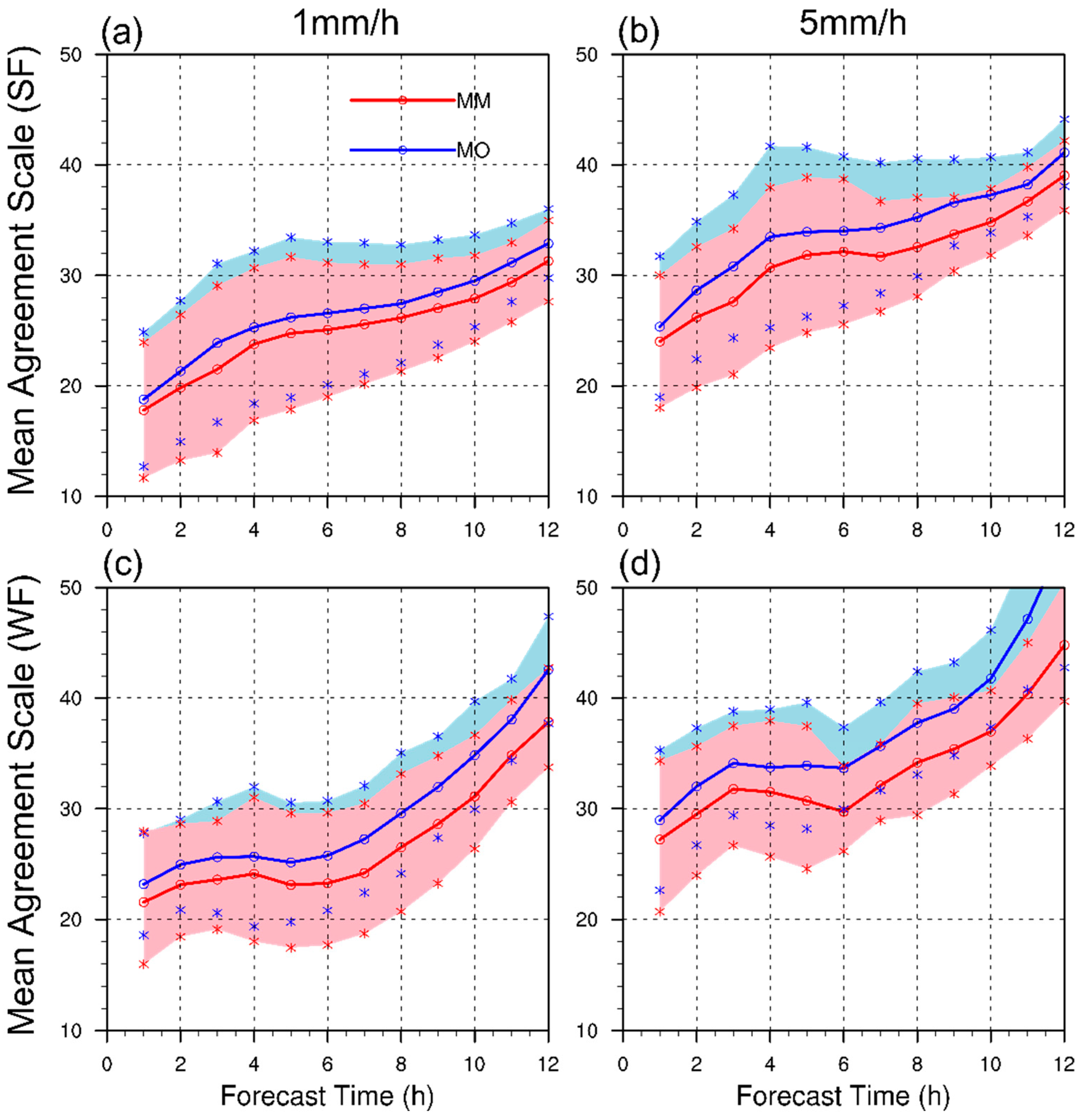
3.2. Spatial Predictability and Spread–Skill Relationship

In this section, the spatial predictability of precipitation forecasts is investigated across convective regimes via EAS in an attempt to provide a better understanding of regime-dependent predictability over the YHRV. Both S_mm and S_mo [15,32] are considered separately to assess the spatial spread–skill for the CSEF derived from flow-dependent ICPs in combination with LBPs. The 1 h precipitation with pre-defined precipitation thresholds (1 mm/h to represent light precipitation events and 5 mm/h to represent stronger events) was used for calibration.

Figure 4 displays the case- and time-averaged spatial distribution of S_mm (Figure 4a–d) and S_mo (Figure 4e–h) for different precipitation thresholds (Figure 4a,c,e,g for 1 mm/h and Figure 4b,d,f,h for 5 mm/h) and different convective regimes (Figure 4a,b,e,f for SF and Figure 4c,d,g,h for WF). Overall, the EAS is larger near the center of convection and gradually increases with decreasing precipitation. This indicates that the EAS method behaved as expected in this study [15]. Additionally, the EAS values of the main EAS centers at higher latitudes under SF are generally lower than those at lower latitude under WF, revealing a higher spatial predictability. This finding is similar to those of Dey et al. [32] and Chen et al. [16], who found that EAS is higher for large coverage precipitation events than for small coverage events. Although we employed a different classification method in this study, the SF (WF) cases were found to correspond well with the larger (smaller) precipitation (see Figure 3) events as in Dey et al. [32] and Chen et al. [16].

Considering the overall spatial spread–skill relationship (Figure 5), S_mm is generally lower than S_mo in the convective region. As shown by the large-area negative bias for both SF and WF, this indicates the under-dispersion issues and is consistent with the findings of Chen et al. [16]. Moreover, the difference between S_mm and S_mo is generally larger for the WF events than for the SF events, especially in mountainous regions. This indicates that the uncertainties for warm-sector convective events are more difficult to estimate than those for typical convective events dominated by the Meiyu front [68], and that the SF events are generally better predicted.

To further investigate the temporal characteristics of the spatial spread–skill, Figure 6 illustrates the evolution of the domain-averaged S_mm and S_mo and their standard deviations for SF (top row of Figure 6) and WF events (bottom row of Figure 6) over 12 h. In general, the domain-averaged mean S_mm is smaller than the domain-averaged S_mo in both regimes for the same lead time, which indicates under-dispersion of the CSEF [16,32], with the evolution trend being steeper under WF than under SF. This suggests that it is desirable to preserve some information in the post-processing processes. The evolution trend of deviation for S_mm and S_mo has a larger range for SF events at early lead times (1–5 h) and for WF events at later lead times (6–12 h), especially for the higher precipitation threshold (Figure 6b,d). This can be explained by the upscale growth of initial error. As documented in previous studies, the flow-dependent initial error can grow rapidly in moist regions driven by moisture dynamics [11,12,69]. Specifically, the rapid displacement of individual cells driven by large-scale forced air ascent around the Meiyu front promotes the upscale error growth of initial small errors [44] and can lead to higher variation of EAS while reaching saturation within early lead time. On the contrary, warm-sector events, which are generally driven by local factors (such as orographic, radiative, or cold-pool factors) [57,66], can lead to consistent local error growth [43,69]. Thus, the EAS shows a larger variation with time, posing challenges for the forecasting of such events.

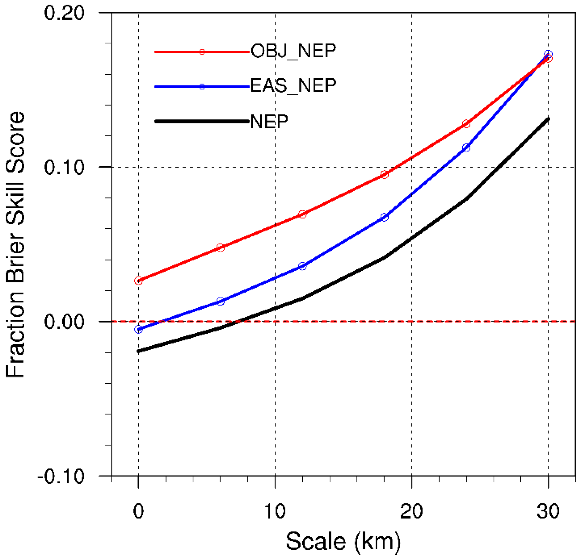
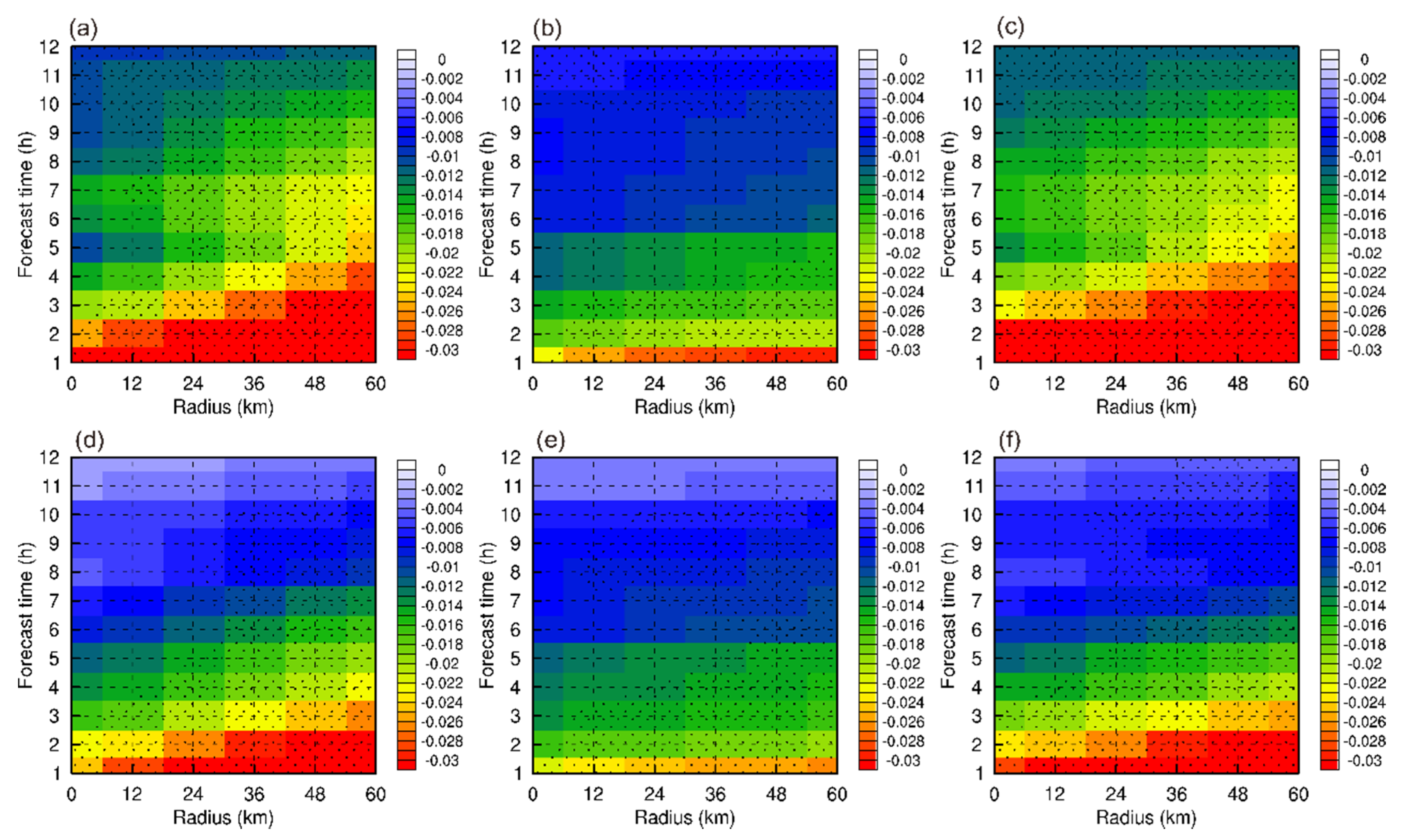
3.3. Verification of Probability Forecasts

Since the regime-dependent spread–skill relationship was found to be highly relevant to the spatial predictability, with a lower spread–skill being associated with lower predictability (i.e., a higher EAS in moist areas), convective events with a lower spatial predictability are associated with a lower grid-based probability. Except for the decay at the maximum probability value (where most ensemble members matched well), the traditional NEP underestimates the probability of precipitation in the small region with the spatial filter. Therefore, in order to achieve regime-dependent predictability in the YHRV (as discussed in Section 3.2) as a result of the growth of nonlinear convective-scale error, the OBJ_NEP method was developed and verified using both idealized experiments and ensemble outputs from WRF-EnKF systems.

3.3.1. Idealized Experiment

First, an idealized experiment was conducted to obtain a better understanding of the advantages and disadvantages of each probabilistic method (GP, NEP, EAS_NEP, and OBJ_NEP). Under a highly idealized condition, two independent events were simulated over the YHRV region (Figure 5a): the first event (OBS1) occurred at a higher latitude and over a larger area, and could be predicted by most ensemble members (greater overlaps) in the CSEF with allowable spatial error, representing the approximate condition of SF (Figure 4a); the second event (OBS2) had a smaller area and occurred at a lower latitude between Tapie Mountain, Huang Mountain, and Mubu Mountain, representing the approximate condition under WF with a lower predictability (only three of the 20 ensemble members capture the cell). At most times, such idealized conditions will not occur. Therefore, the predictive ability of the ensemble members will not be as good (poor) for the former (later) conditions. Both the ensemble members and observations were depicted as simple binary geometric objects with different sizes, representing the binary convection forecasts with a certain precipitation threshold [15].

For OBS1, GP gave higher probabilities, exceeding 60% at the maximum center (Figure 7a), while NEP (Figure 7b), EAS_NEP (Figure 7c), and OBJ_NEP (Figure 7c) had more overlap with OBS1 than GP, indicating that these methods were more effective at representing spatial uncertainties, as expected [26]. Specifically, among the three fraction-based methods, EAS_NEP was the most able to retain the maximum center.

For OBS2, for which there are only a few predictable members, GP exhibits lower probabilities (only exceeding 10–20%). Under these circumstances, the EAS is so large that the probabilistic forecasts are almost filtered out for NEP (Figure 8b) and EAS_NEP (Figure 8c). However, the newly proposed OBJ_NEP method (Figure 8d) shows a better description of OBS2, retaining the smaller forecast objects with a linear dependence between the influence radius and the objects’ size.

To assess the performance of different probabilistic forecasting approaches, plots of the fractions Brier skill score (FBSS) of different probabilistic forecasts as a function of spatial influence scale were created over the inner domain (Figure 8; LBCs excluded). The observation probabilities were generated at each spatial scale, and the GP was used as the reference forecast in Equation 7. Generally, the three fraction-based methods outperform GS, except for NEP and EAS_NEP at spatial scales lower that 6 km. Compared with other approaches, the FBSS curve for OBJ_NEP implies obvious advantages. The OBJ_NEP method effectively shows both maximum centers and spatial uncertainties for OBS1 and retains the small-area probabilities for OBS2. In conclusion, OBJ_NEP combines the advantage of GP for retaining the small-area information and the advantage of EAS_NEP for employing an adaptive radius to each grid.

3.3.2. WRF-EnKF CSEF Experiment

To further verify the effectiveness of OBJ_NEP in ‘real’ case studies, probabilistic methods were objectively compared using outputs from WRF-EnKF (Section 2.2). The radius for EAS_NEP was obtained from the S_mm in Section 3.2 (range from 4 to 64 km), while the NEP was calculated using a medium radius of 32 km to avoid substantial decay at maximum probability centers. For OBJ_NEP, the radius range was also chosen to be between 4 and 64 km, i.e., corresponding to that of EAS_NEP. Bootstrap confidence intervals at the the 90% level for the difference between each spatial-based method and the GP were computed using 1000 replications to assess the statistical significance. A relatively low confidence level was chosen due to the limited number of cases for each subset, and follows the choice of Johnson and Wang [53].

Plots of FBS as a function of horizontal scale and forecast lead time were created for precipitation thresholds of 1 mm/h and 5 mm/h under SF and WF, respectively (Figure 9). The corresponding probability of observation was generated for spatial scales of 0, 12, 24, 36, 48, and 60 km. In general, all of the spatial-based methods showed clear advantages over the traditional GP method, with most of the areas passing the 85% significance level. These advantages are basically related to early lead times with larger spatial scales, due to the fact that the dispersion for ensemble members is generally lower at early lead times, when the spatial-based probability captures more spatial uncertainties (this could also explain the advantages at larger scales) without apparent decay at high-confidence probabilistic centers. However, at later lead times, with the consistent growth of initial error characterized by moist convection and large-scale flow [70], the ensemble members gradually evolve in different directions, leading to lower probabilistic values. Under such circumstances, the effect of added uncertainties extracted with spatial-based methods is clearly reduced [31].

Specifically, EAS_NEP (Figure 9b,e) shows the lowest skill at early lead time compared with NEP and OBJ_NEP. This can be explained by the lower EAS value computed among ensemble members (as depicted in Figure 6, the EAS generally increased with time). Since this research only focused on uncertainties induced by IC and LBCs, the EAS_NEP should have better skill at early lead times computed from CSEF outputs with consideration of model uncertainties [31]. At later lead times, EAS_NEP has higher skill (especially for strong precipitation events with a threshold of 5 mm/h, Figure 9e). This is due to the fact that, at later lead times with lower probability (owing to the upscale error growth), the EAS could effectively retain the probabilities of potentially well-handled events with the application of a smaller radius and adopt a larger radius for poorly-handled events. Additionally, for weaker precipitation events (1 mm/h), EAS_NEP generally shows a lower FBS (Figure 9b) since such incidents are generally excessively widespread in our analysis domain (as indicated in Figure 1b), which leads to a strong constraint of probabilistic skills for EAS_NEP.

The new method, OBJ_NEP (Figure 9c,f), generally obtained a higher FBS, with most areas passing the 90% significance test. During the entire forecast, OBJ_NEP showed an advantage over NEP (Figure 9a,d) at small scales (less than 36 km) for both weak and strong precipitation events. This is due to the effective retaining of smaller-scale forecasting objects with an adaptive object-selective radius, as well as the sufficient representation of spatial uncertainties for larger-scale objects.

For the WF events (Figure 10), the overall advantages of the three spatial-based methods over GP were much weaker than those for the SF events (Figure 9). This can be explained by the lower predictability and under-dispersion issues of the CSEF (see Figure 4 and Figure 5). Additionally, the variation in skill between the spatial-based approaches is similar to that for SF events, further demonstrating the effectiveness of OBJ_NEP.

Furthermore, the AUC score was analyzed as a function of forecast lead time (Figure 11) in order to evaluate the discriminatory ability of GP, NEP, and the two mutative-scale methods. Generally, except for GS at later forecast lead times (Figure 11c,d), the AUC scores for both probabilistic forecasts were greater than 0.7, indicating “useful” forecasts [17]. Moreover, the AUC scores decreased with time, representing the decrease of predictability with consistent error growth.

Regarding the variation of the convective regime, the AUC scores under SF were generally higher (lower) than those under WF within 1–2 h (2–12 h), highlighting the lower predictability of convection under WF. This result is in accordance with the evolution of EAS (Figure 6) and with previous studies [61,71]. It was also observed that the AUC score of GS was clearly lower under WF than under SF, and that the spatial-based methods solved the decay to similar degrees, implying the necessity to apply such methods during the post-processing of CSEFs, especially under WF conditions.

As with the FBS, both of the three spatial-based approaches showed advantages over GS. The associated differences in probabilistic forecast were statistically significant at almost all lead times in both SF and WF regimes, except for SF events with a precipitation threshold of 1 mm/h. Additionally, the three spatial-based methods all led to an eventual divergence with GS, again highlighting that the spatial-based post-processing method can be used to increase the probabilistic forecast skill [17,31].

4. Discussion and Conclusions

This study investigated the regime-dependent spatial predictability and spread–skill relationship in terms of the ensemble agreement scale (EAS) [15,32] over the Yangtze and Huai river valleys (YHRV) using WRF-EnKF convective-scale ensemble forecasts (CSEFs). Furthermore, an object-based probabilistic approach was proposed to fully utilize the spatial-based method as a supplement to the NEP [17] and EAS_NEP [31]. Since CSEFs have been more frequently implemented in recent years, these two goals can aid the better understanding of spatial-based post-processing methods. The contribution of our study to these two goals is as follows:

(1)

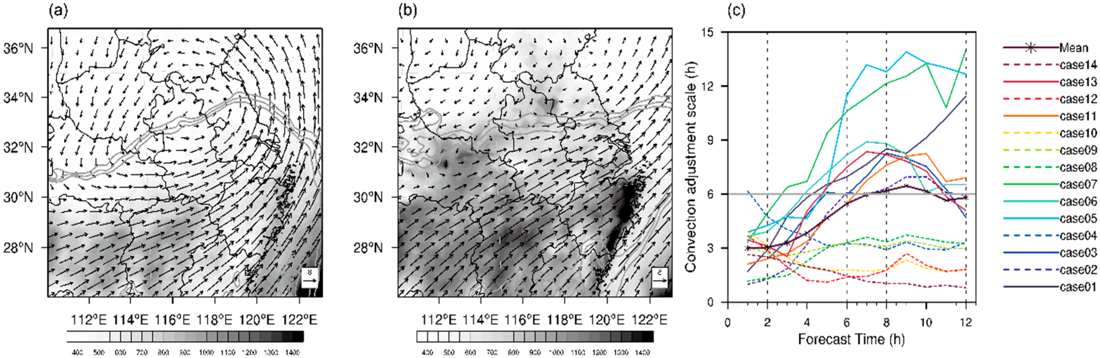
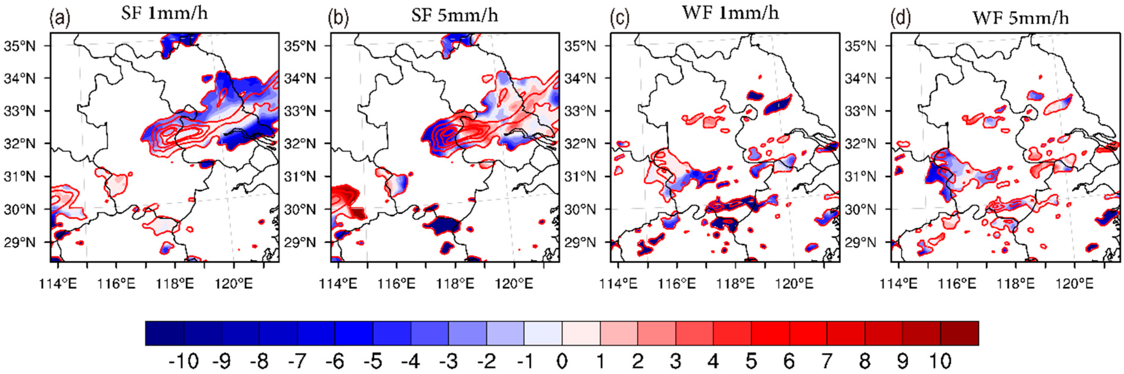
Using the convective adjustment timescale proposed by Done et al. [60] to distinguish convective regimes as strong forcing (SF) and weak forcing (WF) events over the YHRV;

(2)

Applying the EAS proposed by Dey et al. [15,32] to assess the spatial predictability and spread–skill under different convective regimes;

(3)

Offering a new probabilistic forecast approach using an object-based method, fully considering regime-dependent predictability;

(4)

Verifying the effectiveness of the new probabilistic forecast approach in both idealized and true events using the fraction Brier score (FBS) and area under curve (AUC) score.

Our results show that the precipitation characteristics are regime-dependent over the YHRV in the warm season. Convective events under SF were found to generally develop along the Meiyu front, in accordance with Sun and Zhang [36]. However, events under WF were found to mainly develop at lower latitudes around Tapie, Huang, and Mubu mountains (i.e., the warm sector of the YHRV [68]).

Additionally, the associated spatial predictability and spread–skill relationship were also found to be regime-dependent. Regarding the spatial predictability, WF events showed less predictability than SF events, as the EASs in the moist area are generally smaller under SF. These findings are consistent with Dey et al. [32] and Chen et al. [16], thus supporting the effectiveness of the EAS employed in this study. Regarding the spread–skill relationship, both SF and WF events showed under-dispersion issues [11,16], suggesting the need to employ a spatial-based approach to post-processing processes of CSEFs. Moreover, divergence was induced by the time variation of EAS between SF and WF, with the WF (SF) phase having a higher (lower) growth rate and a wider (narrower) trend of deviation among each subset. This can be explained by the dynamics of nonlinear upscale error growth [43,71].

Fully considering regime-dependent features, a new spatial-based probabilistic method (OBJ_NEP) based on a combination of object- and fraction-based methods was proposed to aid the understanding of the post-processing of CSEFs implemented in the YHRV. This new method was assessed using a highly idealized scenario in which a precipitation event with larger (smaller) coverage occurred at higher (lower) latitudes in the YHRV. Although location bias was present, the ensemble members appropriately captured the larger-coverage event; however, only a few members captured the smaller-coverage event. The results show that OBJ_NEP captures both the large-coverage and small-coverage events, while NEP and EAS_NEP do not capture the small-coverage event due to spatial filtering. Further comparison between these probabilistic methods for a ‘real’ scenario using the FBS demonstrated that OBJ_NEP has advantages over NEP at a smaller scale during almost the entire forecast range for both high- and low-impact precipitation events. This advantage is more notable under WF, when severe weather is rare and typically occurs over smaller spatial and temporal scales, revealing that the effective retaining of higher-value and smaller-scale probabilistic information is important. This conclusion could be further supported by the implementation of EAS_NEP, as this model shows more skill under WF with high-impact events than that under SF [17]. Additionally, although only small differences in AUC score were observed among the three spatial-based approaches, NEP, EAS_NEP, and OBJ_NEP all had significantly higher AUC scores than GP.

The results of this study further showed that EAS_NEP does not have superior object verification compared to the traditional NEP method. This may be due to the fact that CSEFs used in this study have lower dispersion than that used in Blake et al. [32] due to OSSE configuration, which leads to a restraint of EAS, especially for early forecast lead times. In future research, we plan to apply and compare the three fraction-based probabilistic approaches, NEP, EAS_NEP, and OBJ_NEP using the 2018 CAPS (Center for Analysis and Prediction of Storms) Spring Forecast Experiments. The products from these experiments have a 3-km grid spacing over the CONUS domain, with ICPs (derived from GSI-EnKF radar assimilation), LBPs (derived from NCEP short-range ensemble forecast products), and a multi-physics configuration, and can provide a more reasonable ensemble spread over a sufficiently large domain.

References

1. Peralta, C.; Ben Bouallègue, Z.; Theis, S.E.; Gebhardt, C.; Buchhold, M. Accounting for initial condition uncertainties in COSMO-DE-EPS. J. Geophys. Res. Atmos. 2012, 117. [Google Scholar] [CrossRef]
2. Nuissier, O.; Joly, B.; Vié, B.; Ducrocq, V. Uncertainty of lateral boundary conditions in a convection-permitting ensemble: A strategy of selection for Mediterranean heavy precipitation events. Nat. Hazards Earth Syst. Sci. 2012, 12, 2993. [Google Scholar] [CrossRef]
3. Harnisch, F.; Keil, C. Initial Conditions for Convective-Scale Ensemble Forecasting Provided by Ensemble Data Assimilation. Mon. Weather Rev. 2015, 143, 1583–1600. [Google Scholar] [CrossRef]
4. Caron, J.-F. Mismatching Perturbations at the Lateral Boundaries in Limited-Area Ensemble Forecasting: A Case Study. Mon. Weather Rev. 2013, 141, 356–374. [Google Scholar] [CrossRef]
5. Tennant, W. Improving initial condition perturbations for MOGREPS-UK. Q. J. R. Meteorol. Soc. 2015, 141, 2324–2336. [Google Scholar] [CrossRef]
6. Vié, B.; Nuissier, O.; Ducrocq, V. Cloud-Resolving Ensemble Simulations of Mediterranean Heavy Precipitating Events: Uncertainty on Initial Conditions and Lateral Boundary Conditions. Mon. Weather Rev. 2011, 139, 403–423. [Google Scholar] [CrossRef]
7. Bouttier, F.; Vié, B.; Nuissier, O.; Raynaud, L. Impact of Stochastic Physics in a Convection-Permitting Ensemble. Mon. Weather Rev. 2012, 140, 3706–3721. [Google Scholar] [CrossRef]
8. Zhang, F.; Bei, N.; Rotunno, R.; Snyder, C.; Epifanio, C.C. Mesoscale Predictability of Moist Baroclinic Waves: Convection-Permitting Experiments and Multistage Error Growth Dynamics. J. Atmos. Sci. 2007, 64, 3579–3594. [Google Scholar] [CrossRef]
9. Selz, T.; Craig, G.C. Upscale Error Growth in a High-Resolution Simulation of a Summertime Weather Event over Europe. Mon. Weather Rev. 2015, 143, 813–827. [Google Scholar] [CrossRef]
10. Surcel, M.; Zawadzki, I.; Yau, M.K. A Study on the Scale Dependence of the Predictability of Precipitation Patterns. J. Atmos. Sci. 2015, 72, 216–235. [Google Scholar] [CrossRef]
11. Sun, Y.Q.; Zhang, F. Intrinsic versus Practical Limits of Atmospheric Predictability and the Significance of the Butterfly Effect. J. Atmos. Sci. 2016, 73, 1419–1438. [Google Scholar] [CrossRef] [Green Version]
12. Zhang, X. Multiscale Characteristics of Different-Source Perturbations and Their Interactions for Convection-Permitting Ensemble Forecasting during SCMREX. Mon. Weather Rev. 2019, 147, 291–310. [Google Scholar] [CrossRef]
13. Romine, G.S.; Schwartz, C.S.; Berner, J.; Fossell, K.R.; Snyder, C.; Anderson, J.L.; Weisman, M.L. Representing Forecast Error in a Convection-Permitting Ensemble System. Mon. Weather Rev. 2014, 142, 4519–4541. [Google Scholar] [CrossRef] [Green Version]
14. Schwartz, C.S.; Romine, G.S.; Smith, K.R.; Weisman, M.L. Characterizing and Optimizing Precipitation Forecasts from a Convection-Permitting Ensemble Initialized by a Mesoscale Ensemble Kalman Filter. Weather Forecast. 2014, 29, 1295–1318. [Google Scholar] [CrossRef] [Green Version]
15. Dey, S.R.A.; Plant, R.S.; Roberts, N.M.; Migliorini, S. Assessing spatial precipitation uncertainties in a convective-scale ensemble. Q. J. R. Meteorol. Soc. 2016, 142, 2935–2948. [Google Scholar] [CrossRef]
16. Chen, X.; Yuan, H.; Xue, M. Spatial spread–skill relationship in terms of agreement scales for precipitation forecasts in a convection-allowing ensemble. Q. J. R. Meteorol. Soc. 2018, 144, 85–98. [Google Scholar] [CrossRef]
17. Schwartz, C.S.; Sobash, R.A. Generating Probabilistic Forecasts from Convection-Allowing Ensembles Using Neighborhood Approaches: A Review and Recommendations. Mon. Weather Rev. 2017, 145, 3397–3418. [Google Scholar] [CrossRef]
18. Wang, X.; Bishop, C.H. A Comparison of Breeding and Ensemble Transform Kalman Filter Ensemble Forecast Schemes. J. Atmos. Sci. 2003, 60, 1140–1158. [Google Scholar] [CrossRef]
19. Wang, X.; Bishop, C.H.; Julier, S.J. Which Is Better, an Ensemble of Positive–Negative Pairs or a Centered Spherical Simplex Ensemble? Mon. Weather Rev. 2004, 132, 1590–1605. [Google Scholar] [CrossRef]
20. Wang, Y.; Tascu, S.; Weidle, F.; Schmeisser, K. Evaluation of the Added Value of Regional Ensemble Forecasts on Global Ensemble Forecasts. Weather Forecast. 2012, 27, 972–987. [Google Scholar] [CrossRef]
21. Zhang, H.; Chen, J.; Zhi, X.; Wang, Y. A Comparison of ETKF and Downscaling in a Regional Ensemble Prediction System. Atmosphere 2015, 6, 341–360. [Google Scholar] [CrossRef]
22. Weidle, F.; Wang, Y.; Smet, G. On the Impact of the Choice of Global Ensemble in Forcing a Regional Ensemble System. Weather Forecast. 2016, 31, 515–530. [Google Scholar] [CrossRef]
23. Gilleland, E.; Ahijevych, D.; Brown, B.G.; Casati, B.; Ebert, E.E. Intercomparison of Spatial Forecast Verification Methods. Weather Forecast. 2009, 24, 1416–1430. [Google Scholar] [CrossRef]
24. Mittermaier, M.; Roberts, N.; Thompson, S.A. A long-term assessment of precipitation forecast skill using the Fractions Skill Score. Meteorol. Appl. 2013, 20, 176–186. [Google Scholar] [CrossRef]
25. Johnson, A.; Wang, X. Object-Based Evaluation of a Storm-Scale Ensemble during the 2009 NOAA Hazardous Weather Testbed Spring Experiment. Mon. Weather Rev. 2013, 141, 1079–1098. [Google Scholar] [CrossRef]
26. Roberts, N.M.; Lean, H.W. Scale-Selective Verification of Rainfall Accumulations from High-Resolution Forecasts of Convective Events. Mon. Weather Rev. 2008, 136, 78–97. [Google Scholar] [CrossRef]
27. Mittermaier, M.; Roberts, N. Intercomparison of Spatial Forecast Verification Methods: Identifying Skillful Spatial Scales Using the Fractions Skill Score. Weather Forecast. 2010, 25, 343–354. [Google Scholar] [CrossRef]
28. Dey, S.R.A.; Leoncini, G.; Roberts, N.M.; Plant, R.S.; Migliorini, S. A Spatial View of Ensemble Spread in Convection Permitting Ensembles. Mon. Weather Rev. 2014, 142, 4091–4107. [Google Scholar] [CrossRef] [Green Version]
29. Clark, A.J.; Gao, J.; Marsh, P.T.; Smith, T.; Kain, J.S.; Correia, J.; Xue, M.; Kong, F. Tornado Pathlength Forecasts from 2010 to 2011 Using Ensemble Updraft Helicity. Weather Forecast. 2013, 28, 387–407. [Google Scholar] [CrossRef] [Green Version]
30. Zhu, K.; Yang, Y.; Xue, M. Percentile-based neighborhood precipitation verification and its application to a landfalling tropical storm case with radar data assimilation. Adv. Atmos. Sci. 2015, 32, 1449–1459. [Google Scholar] [CrossRef]
31. Blake, B.T.; Carley, J.R.; Alcott, T.I.; Jankov, I.; Pyle, M.E.; Perfater, S.E.; Albright, B. An Adaptive Approach for the Calculation of Ensemble Gridpoint Probabilities. Weather Forecast. 2018, 33, 1063–1080. [Google Scholar] [CrossRef]
32. Dey, S.R.A.; Roberts, N.M.; Plant, R.S.; Migliorini, S. A new method for the characterization and verification of local spatial predictability for convective-scale ensembles. Q. J. R. Meteorol. Soc. 2016, 142, 1982–1996. [Google Scholar] [CrossRef] [Green Version]
33. Davis, C.; Brown, B.; Bullock, R. Object-Based Verification of Precipitation Forecasts. Part I: Methodology and Application to Mesoscale Rain Areas. Mon. Weather Rev. 2006, 134, 1772–1784. [Google Scholar] [CrossRef] [Green Version]
34. Davis, C.A.; Brown, B.G.; Bullock, R.; Halley-Gotway, J. The Method for Object-Based Diagnostic Evaluation (MODE) Applied to Numerical Forecasts from the 2005 NSSL/SPC Spring Program. Weather Forecast. 2009, 24, 1252–1267. [Google Scholar] [CrossRef] [Green Version]
35. Gallus, W.A. Application of Object-Based Verification Techniques to Ensemble Precipitation Forecasts. Weather Forecast. 2010, 25, 144–158. [Google Scholar] [CrossRef] [Green Version]
36. Sun, J.; Zhang, F. Impacts of Mountain–Plains Solenoid on Diurnal Variations of Rainfalls along the Mei-Yu Front over the East China Plains. Mon. Weather Rev. 2012, 140, 379–397. [Google Scholar] [CrossRef]
37. Ding, Y.; Chan, J.C. The East Asian summer monsoon: An overview. Meteorol. Atmos. Phys. 2005, 89, 117–142. [Google Scholar]
38. Luo, Y.; Qian, W.; Zhang, R. Gridded hourly precipitation analysis from high-density rain gauge network over the Yangtze-Huai rivers basin during the 2007 Meiyu season and comparison with CMORPH. J. Hydrometeorol. 2013, 14, 1243–1258. [Google Scholar] [CrossRef]
39. Martin, W.J.; Xue, M. Sensitivity Analysis of Convection of the 24 May 2002 IHOP Case Using Very Large Ensembles. Mon. Weather Rev. 2006, 134, 192–207. [Google Scholar] [CrossRef] [Green Version]
40. Li, H.; Cui, X.; Zhang, D.-L. Sensitivity of the initiation of an isolated thunderstorm over the Beijing metropolitan region to urbanization, terrain morphology and cold outflows. Q. J. R. Meteorol. Soc. 2017, 143, 3153–3164. [Google Scholar] [CrossRef]
41. Keil, C.; Heinlein, F.; Craig, G.C. The convective adjustment time-scale as indicator of predictability of convective precipitation. Q. J. R. Meteorol. Soc. 2014, 140, 480–490. [Google Scholar] [CrossRef]
42. Johnson, A.; Wang, X.; Carley, J.R.; Wicker, L.J.; Karstens, C. A comparison of multiscale GSI-based EnKF and 3DVar data assimilation using radar and conventional observations for midlatitude convective-scale precipitation forecasts. Mon. Weather Rev. 2015, 143, 3087–3108. [Google Scholar] [CrossRef]
43. Flack, D.L.A.; Gray, S.L.; Plant, R.S.; Lean, H.W.; Craig, G.C. Convective-Scale Perturbation Growth across the Spectrum of Convective Regimes. Mon. Weather Rev. 2018, 146, 387–405. [Google Scholar] [CrossRef]
44. Skamarock, W.C.; Klemp, J.B.; Dudhia, J.; Gill, D.O.; Barker, D.M.; Duda, M.G.; Huang, X.-Y.; Wang, W.; Powers, J.G. A Description of the Advanced Research WRF Version 3, NCAR Technical Note; National Center for Atmospheric Research: Boulder, CO, USA, 2008. [Google Scholar]
45. Grasso, L.; Lindsey, D.T.; Lim, K.-S.S.; Clark, A.; Bikos, D.; Dembek, S.R. Evaluation of and Suggested Improvements to the WSM6 Microphysics in WRF-ARW Using Synthetic and Observed GOES-13 Imagery. Mon. Weather Rev. 2014, 142, 3635–3650. [Google Scholar] [CrossRef]
46. Grell, G.A.; Dévényi, D. A generalized approach to parameterizing convection combining ensemble and data assimilation techniques. Geophys. Res. Lett. 2002, 29, 38-1–38-4. [Google Scholar] [CrossRef]
47. Hong, S.-Y.; Noh, Y.; Dudhia, J. A New Vertical Diffusion Package with an Explicit Treatment of Entrainment Processes. Mon. Weather Rev. 2006, 134, 2318–2341. [Google Scholar] [CrossRef] [Green Version]
48. Mlawer, E.J.; Taubman, S.J.; Brown, P.D.; Iacono, M.J.; Clough, S.A. Radiative transfer for inhomogeneous atmospheres: RRTM, a validated correlated-k model for the longwave. J. Geophys. Res. D Atmos. 1997, 102, 16663–16682. [Google Scholar] [CrossRef] [Green Version]
49. Chou, M.-D.; Suarez, M.J. A solar radiation parameterization (CLIRAD-SW) for atmospheric studies. NASA Tech. Memo. 1999, 15, 48. [Google Scholar]
50. Whitaker, J.S.; Hamill, T.M. Ensemble Data Assimilation without Perturbed Observations. Mon. Weather Rev. 2002, 130, 1913–1924. [Google Scholar] [CrossRef]
51. Hagedorn, R.; Hamill, T.M.; Whitaker, J.S. Probabilistic Forecast Calibration Using ECMWF and GFS Ensemble Reforecasts. Part I: Two-Meter Temperatures. Mon. Weather Rev. 2008, 136, 2608–2619. [Google Scholar] [CrossRef]
52. Hagedorn, R.; Buizza, R.; Hamill, T.M.; Leutbecher, M.; Palmer, T.N. Comparing TIGGE multimodel forecasts with reforecast-calibrated ECMWF ensemble forecasts. Q. J. R. Meteorol. Soc. 2012, 138, 1814–1827. [Google Scholar] [CrossRef]
53. Johnson, A.; Wang, X. A Study of Multiscale Initial Condition Perturbation Methods for Convection-Permitting Ensemble Forecasts. Mon. Weather Rev. 2016, 144, 2579–2604. [Google Scholar] [CrossRef]
54. Gasperoni, N.A.; Xue, M.; Palmer, R.D.; Gao, J. Sensitivity of Convective Initiation Prediction to Near-Surface Moisture When Assimilating Radar Refractivity: Impact Tests Using OSSEs. J. Atmos. Ocean. Technol. 2013, 30, 2281–2302. [Google Scholar] [CrossRef]
55. Madaus, L.E.; Hakim, G.J. Constraining Ensemble Forecasts of Discrete Convective Initiation with Surface Observations. Mon. Weather Rev. 2017, 145, 2597–2610. [Google Scholar] [CrossRef]
56. Anderson, J.L.; Anderson, S.L. A Monte Carlo Implementation of the Nonlinear Filtering Problem to Produce Ensemble Assimilations and Forecasts. Mon. Weather Rev. 1999, 127, 2741–2758. [Google Scholar] [CrossRef]
57. Tong, M.; Xue, M. Ensemble Kalman Filter Assimilation of Doppler Radar Data with a Compressible Nonhydrostatic Model: OSS Experiments. Mon. Weather Rev. 2005, 133, 1789–1807. [Google Scholar] [CrossRef] [Green Version]
58. Zhang, F.; Snyder, C.; Sun, J. Impacts of Initial Estimate and Observation Availability on Convective-Scale Data Assimilation with an Ensemble Kalman Filter. Mon. Weather Rev. 2004, 132, 1238–1253. [Google Scholar] [CrossRef]
59. Liu, J.Y.; Tan, Z.M.; Zhang, Y. Study of the three types of torrential rains of different formation mechanism during the Meiyu period. Acta Meteorol. Sin. 2012, 70, 452–466. [Google Scholar]
60. Done, J.M.; Craig, G.C.; Gray, S.L.; Clark, P.A.; Gray, M.E.B. Mesoscale simulations of organized convection: Importance of convective equilibrium. Q. J. R. Meteorol. Soc. 2006, 132, 737–756. [Google Scholar] [CrossRef] [Green Version]
61. Done, J.M.; Craig, G.C.; Gray, S.L.; Clark, P.A. Case-to-case variability of predictability of deep convection in a mesoscale model. Q. J. R. Meteorol. Soc. 2012, 138, 638–648. [Google Scholar] [CrossRef]
62. Flack, D.L.A.; Plant, R.S.; Gray, S.L.; Lean, H.W.; Keil, C.; Craig, G.C. Characterisation of convective regimes over the British Isles. Q. J. R. Meteorol. Soc. 2016, 142, 1541–1553. [Google Scholar] [CrossRef]
63. Surcel, M.; Zawadzki, I.; Yau, M.K.; Xue, M.; Kong, F. More on the Scale Dependence of the Predictability of Precipitation Patterns: Extension to the 2009–13 CAPS Spring Experiment Ensemble Forecasts. Mon. Weather Rev. 2017, 145, 3625–3646. [Google Scholar] [CrossRef]
64. Schwartz, C.S.; Kain, J.S.; Weiss, S.J.; Xue, M.; Bright, D.R.; Kong, F.; Thomas, K.W.; Levit, J.J.; Coniglio, M.C.; Wandishin, M.S. Toward Improved Convection-Allowing Ensembles: Model Physics Sensitivities and Optimizing Probabilistic Guidance with Small Ensemble Membership. Weather Forecast. 2010, 25, 263–280. [Google Scholar] [CrossRef]
65. Brier, G.W. The Statistical Theory of Turbulence and the Problem of Diffusion in the Atmosphere. J. Atmos. Sci. 1950, 7, 283–290. [Google Scholar] [CrossRef]
66. Wandishin, M.S.; Mullen, S.J. Multiclass ROC Analysis. Weather Forecast. 2009, 24, 530–547. [Google Scholar] [CrossRef]
67. Marzban, C. The ROC Curve and the Area under It as Performance Measures. Weather Forecast. 2004, 19, 1106–1114. [Google Scholar] [CrossRef]
68. Chen, Y.; Chan, Y.; Chen, T.; He, H. Characteristics analysis of warm-sector rainstorms over the middle-lowers reaches of the Yangtze River. Meteorol. Mon. 2016, 42, 724–731. (In Chinese) [Google Scholar]
69. Hohenegger, C.; Schar, C. Atmospheric Predictability at Synoptic Versus Cloud-Resolving Scales. Bull. Am. Meteorol. Soc. 2007, 88, 1783–1794. [Google Scholar] [CrossRef]
70. Nielsen, E.R.; Schumacher, R.S. Using Convection-Allowing Ensembles to Understand the Predictability of an Extreme Rainfall Event. Mon. Weather Rev. 2016, 144, 3651–3676. [Google Scholar] [CrossRef]
71. Klasa, C.; Arpagaus, M.; Walser, A.; Wernli, H. On the Time Evolution of Limited-Area Ensemble Variance: Case Stud. with the Convection-Permitting Ensemble COSMO-E. J. Atmos. Sci. 2019, 76, 11–26. [Google Scholar] [CrossRef]
Figure 1. (a) Configuration of model domain. The red square indicates the inner domain and the black dots show the distribution of the simulated sounding datasets. (b) Terrain height (m) within the inner domain. Blue circles show the coverages of the seven radar sites.
Atmosphere 10 00490 g001
Figure 2. Ensemble-mean case-averaged 850 hPa wind vector (m/s), equivalent potential temperature (344–348 K, 2 K interval, indicative of the location of the Meiyu front) and convective available potential energy (white to black scale, J/Kg) for the (a) strong forcing (SF) and (b) weak forcing (WF) cases. (c) The convective adjustment timescale ( τ c ) averaged over all areas with a rainfall higher than 0.5 mm/h as a function of forecast time (in hours) for 14 heavy rainfall events.
Atmosphere 10 00490 g002
Figure 3. Spatial distributions of 12 h accumulated precipitation (mm) averaged from (a,c) the true state and (b,d) the control forecasts over lead times of 0–12 h for (a,b) SF events and (c,d) WF events.
Atmosphere 10 00490 g003
Figure 4. Case-averaged spatial distribution of (ad) Smm and (eh) Smo averaged over the 1–12 h lead time for (a,b,e,f) SF events and (c,d,g,h) WF events, with precipitation thresholds of (a,c,e,g) 1 mm/h and (b,d,f,h) 5 mm/h. The red contours show the case-averaged 12 h accumulated precipitation which is indicative of moist areas.
Atmosphere 10 00490 g004
Figure 5. Case-averaged spatial distribution of [Smm–Smo] averaged over the 1–12 h lead time for (a,b) SF events and (c,d) WF events, with precipitation thresholds of (a,c) 1 mm/h and (b,d) 5 mm/h. The red contours show the case-averaged 12 h accumulated precipitation which is indicative of moist areas.
Atmosphere 10 00490 g005
Figure 6. Variations of case- and domain-averaged Smm (red line) and Smo (blue line) for (a,b) SF events and (c,d) WF events, with precipitation thresholds of (a,c) 1 mm/h and (b,d) 5 mm/h. The shaded areas represent the standard deviations of different events within certain categories; the red and blue shaded areas represent Smm and Smo, respectively.
Atmosphere 10 00490 g006
Figure 7. Probabilistic forecasts for an idealized experiment for (a) GP, (b) NEP, (c) EAS_NEP, (d) OBJ_NEP. The black contours represent observations.
Atmosphere 10 00490 g007
Figure 8. Graphs of Fractions Brier Skill Score (FBSS) as a function of spatial scale (km) for the NEP (black curve), EAS_NEP (blue curve), and OBJ_NEP (red curve) approaches for the idealized experiment. GP was used as the reference forecast.
Atmosphere 10 00490 g008
Figure 9. Differences between the fractional Brier score (FBS) of (a,d) NEP and GP, (b,e) EAS_NEP and GP, and (c,f) OBJ_NEP and GP with precipitation thresholds of (top) 1 mm/h and (bottom) 5 mm/h under SF. The dotted areas show the 90% bootstrap confidence intervals.
Atmosphere 10 00490 g009
Figure 10. Differences between the fractional Brier score (FBS) of (a,d) NEP and GP, (b,e) EAS_NEP and GP, and (c,f) OBJ_NEP and GP with precipitation thresholds of (top) 1 mm/h and (bottom) 5 mm/h under WF. The dotted areas show the 90% bootstrap confidence intervals.
Atmosphere 10 00490 g010
Figure 11. Graphs of area under curve (AUC) scores as a function of forecast lead time for GP (black line), NEP (gray line), EAS_NEP (blue line), and OBJ_NEP (red line) with a precipitation threshold of (left column) 1 mm/h and (right column) 5 mm/h, under (a,b) SF and (c,d) WF. Solid dots show the 85% bootstrap confidence intervals for differences between each fraction-based method and GP.
Atmosphere 10 00490 g011