Article

Prediction of Air Temperature in the Polish Western Carpathian Mountains with the ALADIN-HIRLAM Numerical Weather Prediction System

1
Faculty of Physics and Applied Computer Science, AGH-University of Science and Technology, 30-059 Krakow, Poland
2
Institute of Meteorology and Water Management, National Research Institute, IMGW-PIB Branch of Krakow, 30-215 Krakow, Poland
3
Institute of Geography and Spatial Management, Jagiellonian University, 30-387 Krakow, Poland
*
Author to whom correspondence should be addressed.
Atmosphere 2019, 10(4), 186; https://doi.org/10.3390/atmos10040186
Submission received: 5 January 2019 / Revised: 25 March 2019 / Accepted: 2 April 2019 / Published: 5 April 2019
(This article belongs to the Section Meteorology)

Abstract

:
Prediction of spatial and temporal variability of air temperature in areas with complex topography is still a challenge for numerical weather prediction models. Simulation of atmosphere over complex terrain requires dense and accurate horizontal and vertical grids. In this study, verification results of three configurations of the Aire Limitée Adaptation Dynamique Développement International High-Resolution Limited Area Model (ALADIN-HIRLAM) numerical weather prediction (NWP) system, using two different horizontal and vertical resolutions and applied to the Polish Western Carpathian Mountains, are presented. One model of the ALADIN-HIRLAM NWP system is tested in two horizontal and vertical resolutions. Predicted air temperatures are compared with observations from stations located in different orographies. A comparison of model results with observations was conducted for three cold season intervals in 2017 and 2018. Statistical validation of model output demonstrates better model representativeness for stations located on hill and mountain tops compared to locations in valley bottoms. A comparison of results for two topography representations (2 × 2 km and 1 × 1 km) showed no statistically significant differences of root mean square error (RMSE) and bias between model results and observations.

1. Introduction

Increasing knowledge about physical atmospheric processes contributes to improvement of the numerical models used for weather forecasting. Tests of new model configurations show that weather prediction for regions with complex topography constitutes a challenging task for the development of numerical weather forecasting (NWF) systems. One internationally coordinated activity is the Transport and Exchange Processes in the Atmosphere over Mountains Experiment (TEAMx) [1]. Regions with highly complex relief are important, not only because of the impact on weather formation, but also the occurrence of processes like katabatic flows and strong temperature inversions caused by stable stratification of the air volume within the valleys. Those processes have a significant impact on air quality, as they stimulate an increased concentration of air pollutants and the formation of smog episodes.
The Aire Limitée Adaptation Dynamique Développement International (ALADIN) High Resolution Limited Area Model (HIRLAM) system is a numerical weather prediction (NWP) system developed by the international ALADIN and HIRLAM consortiums for operational weather forecasting and research purposes [2,3]. The ALADIN-HIRLAM NWP system is based on a code that is shared with the Integrated Forecast System (IFS) global model developed by the European Centre for Medium-Range Weather Forecasts (ECMWF) and the Action de Recherche Petite Echelle Grande Echelle (ARPEGE) global numerical weather prediction model used for operational weather forecasting at Météo-France. The system provides a multitude of high-resolution limited-area model (LAM) configurations. Several configurations in the ALADIN consortium are precisely validated and prepared to be used for operational weather forecasting at the 16 partner institutes. These configurations are called the ALADIN canonical model configurations (CMCs). Currently there are three canonical model configurations: the ALADIN baseline CMC, the Application of Research to Operations at Mesoscale (AROME) CMC, and the ALADIN–AROME (ALARO) CMC. The HIRLAM consortium prepared its own model configuration of AROME, named the HIRLAM ALADIN Regional/Mesoscale Operational NWP in Europe AROME (HARMONIE–AROME), which is used for operational short-range weather forecasts in 10 countries in Europe.
Reliable weather forecasting for such regions may require models of subkilometer spatial resolution. Meteo France is running the AROME operational model with a resolution of 1.3 km [4]. The first results of the preoperational high-resolution AROME model (named AROME Airport) were presented by Hagelin et al. [5]. A rapidly updated forecast was run with 500 m resolution for nowcasting over Paris Charles de Gaulle Airport (CDG) to increase the safety of airport operations. The results of AROME Airport were compared with the operational configuration of the AROME model using the forecasts from AROME Airport starting every hour. The forecasts from AROME Airport delivered improved data compared to the operational version, in particular for wind speed for runs from all forecast hours. ALADIN and HIRLAM consortium members are testing new configurations of sub-km models. For example, the Danish Meteorological Institute, which belongs to the HIRLAM consortium, presented some promising results of the HARMONIE-AROME model with a resolution of 750 m [6]. Changing the resolution of the numerical weather forecast model to the regional scale (i.e., a few hundred meters) is necessary for its verification. Tests of verification of the high-resolution model were presented by Amodei et al. [7]. A regional Brier probability score was used to compare the results from the high-resolution model with those from the low-resolution model in terms of the forecast of rainfall and wind gusts, with application of the observations from surface stations. The method was based on a comparison of the frequency from the forecast with observed events in the neighborhood of each measurement point. High-resolution forecasts of small-scale events are usually correct, but forecasts of these events can be slightly shifted in space and time from observations. Forecasts of events shifted in space and time are penalized twice, because of false alarm and nondetection, which is called double penalty. The adopted strategy reduced the impact of the double penalty, greatly affecting the high-resolution model compared with models at lower resolution.
Poland is one of the European countries with relatively poor air quality, especially during the cold part of the year [8]. Most affected are areas with complex topography where the natural dispersion conditions are often very poor, due to the local weather phenomena mentioned above, especially thermal inversions. The Polish Western Carpathian Mountains represent such a region and were chosen as the study area. The aim of the paper was to evaluate the performance of the operational AROME model in the study region and to verify the hypothesis that in mountain areas, the increased resolution in the ALADIN-HIRLAM NWP system would significantly improve the accuracy of air temperature forecasts (at the level of 2 m above the ground). The AROME model is used by the Polish Institute of Meteorology and Water Management, National Research Institute (IMWM-NRI). Three configurations of the nonoperational ALADIN-HIRLAM NWP system (AROME 1 km × 1 km, ALARO nonhydrostatic (NH) 1 km × 1 km, and HARMONIE-AROME 2 km × 2 km) were used for verification of the above hypothesis. The verification of model forecast results was achieved by comparison with measurements from 19 meteorological stations located in the Western Carpathian Mountains.
The present study consists of four sections. The first section includes a presentation of the context of the issue and a formulation of the research aim. Section 2 contains a brief description of the analyzed region, data and methods used for forecast verification, descriptions of the ALADIN consortium and ALADIN-HIRLAM NWP system, and the representativeness of stations in the model domains. Section 3 shows the results obtained with the AROME CMC operational model and a comparison of the results from different configurations of ALADIN consortium models. Section 4 contains the conclusions.

2. Data and Methodology

2.1. Study Area

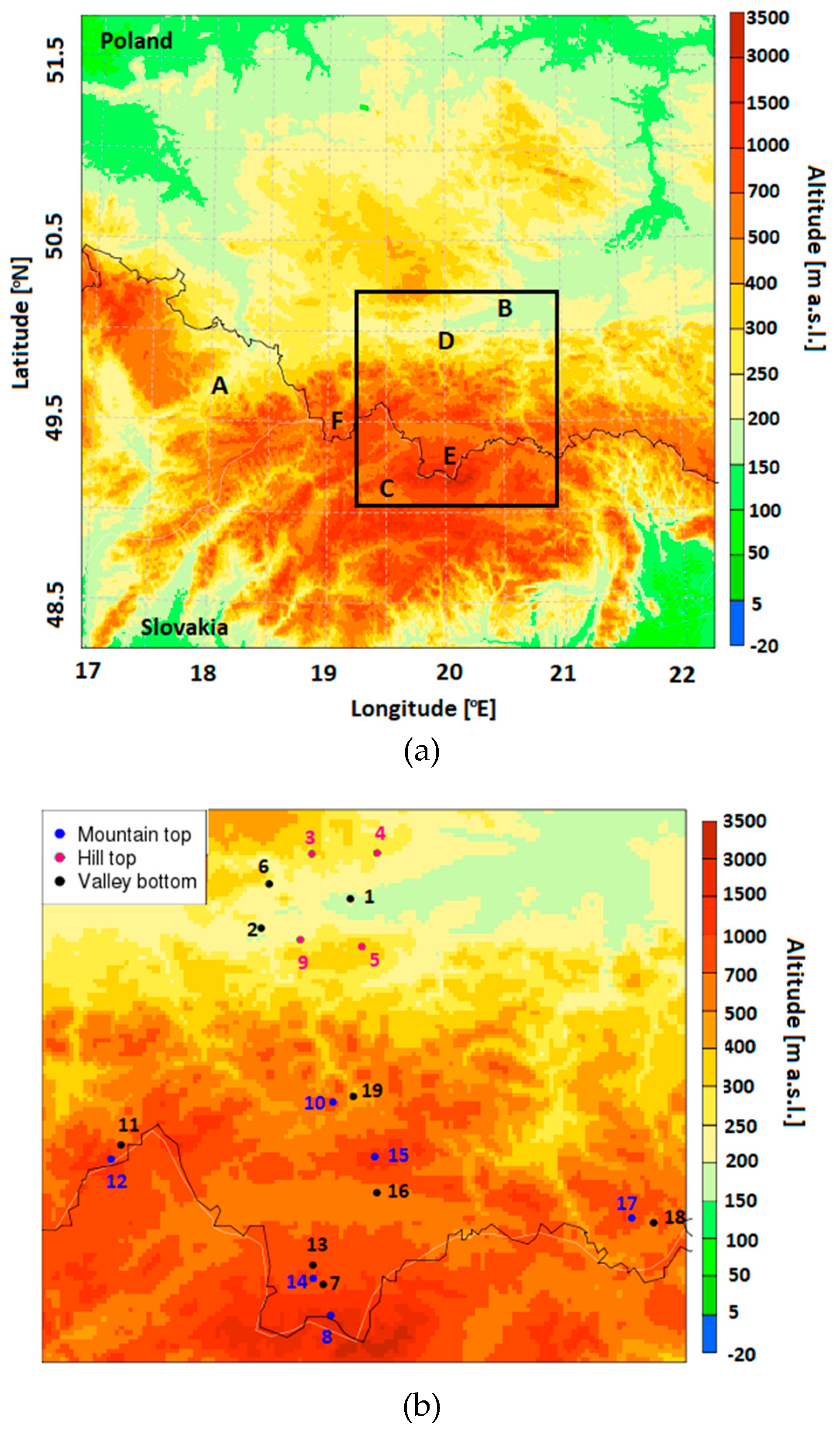
The Polish Western Carpathian Mts. are the northernmost and westernmost parts of the Carpathians, a mountain range located in eight European countries: Austria, the Czech Republic, Hungary, Poland, Romania, Serbia, Slovakia, and Ukraine. The Polish part covers about 6% of the area of the country (1.96 million hectares) and extends from the Moravian Gate (marked as A in Figure 1a) in the west to the Ukrainian Carpathians (beyond the range of Figure 1) in the east, and from the chain of basins in the north (located in the Carpathian Foredeep; B) to the Slovakian Carpathians in the south (C). The altitude varies from 200 to 300 m a.s.l. in the Carpathian Foothills (D) to over 2000 m a.s.l. in the highest range of the whole Carpathians, the Tatra Mts., (E) with the highest peak being Gerlach (2655 m a.s.l., located in Slovakia; the highest Polish peak of the Tatra Mts. is Rysy, 2499 m a.s.l.). The Tatra Mts. are the only part of the Carpathians with typical alpine, high mountain landscape. Farther to the north is the main part of the Polish Western Carpathians, the Beskidy Mts. (divided further into several ranges), with altitudes exceeding 1000 m a.s.l., and the highest peak, Babia Góra Mt., at 1725 m a.s.l., is located in the Beskid Żywiecki Mts. (F). A characteristic feature of the Beskidy Mts.’ relief is the presence of deeply incised valleys, as relative heights reach 400–700 m. The mountain peaks are most often forested and not favorable for settlement. Therefore, human activity is concentrated in the valleys. It is the opposite in the Carpathian Foothills, which extend along the Beskidy Mts. from west to east. They consist of hills with relatively wide and flat hilltops where settlements and transportation infrastructure are located, while the valleys are left unused and often forested. The climatic conditions are very diverse due to the large differences in altitude and complex relief. Mean annual air temperature in the period 1951–2006 varied from 8.0 °C in Kraków (northern border of the foothills) to 5.3 °C in Zakopane (foot of the Tatra Mts.) and −0.6 °C at Kasprowy Wierch Mt. (a peak in the Tatra Mts. at 1987 m a.s.l.). Mean annual precipitation sums varied from 667 mm in Kraków to 1115 mm in Zakopane and 1754 mm at Kasprowy Wierch Mt. [9,10]. Vertical climatic zones are best developed in the Tatra Mts., from a forest zone at the foot of the mountain up to bare rock zone at the highest peaks, but the climatic zonality is also well seen in most of the Beskidy Mt. ranges [11]. Particular weather features of the Polish Western Carpathians include foehn winds [12], air temperature inversions, and the highest mean annual number of days with thunderstorms (up to 34 days in the Tatra Mts.) compared to other regions of Poland [13,14]. The Carpathian valleys show large spatial diversity of local climate, forming a sequence of temperature–humidity vertical zones [15].

2.2. Measurement Data

The study was focused on the cold part of the year (September to April), when heating season takes place. This is linked to the fact that the vertical lapse rate in that part of the year is often decisive for air pollution dispersion, due to the formation of air temperature inversions. Therefore, the study concentrated on the air temperature spatial distribution in the area with diversified relief, where air pollution problems are the greatest, and the application of data from the stations located in the valleys and at the hilltops. The air temperature data from the measurements were available for two uneven periods: 1 January to 3 April 2017 and 1 September 2017 to 30 April 2018. In order to eliminate the effects of various sample sizes, studies on the variability of air temperature (at 2 m above the ground) for the Polish Western Carpathian Mts. were carried out for three intervals: winter/spring, 1 January to 30 April 2017 and 1 January to 30 April 2018, and autumn/winter, 1 September to 31 December 2017. Additionally, the division of subperiods was linked to the fact that for each subperiod, the number of stations from which data were available was different, and merging the data into one sample would eliminate 6 stations from the 19 studied.
Air temperature measurements from 19 meteorological stations or measurement points were used to verify the model forecast. The stations/measurement points are located in both concave and convex land forms (i.e., in valleys and at the tops of hills or mountains) so as to represent the diversity of local climate generated by the complex relief, as described in Section 2. From 19 stations/measurement points mentioned, 13 were owned and maintained by the IMWM-NRI (10 automatic stations and 3 synoptic stations). Five measurement points were located in the vicinity of Kraków and belonged to Jagiellonian University (JU). Basic information about the stations/measurement points is presented in Table 1. Measurement points 1–4 and 6 were located outside the Carpathians but very close to their northern border and, therefore, they were included in the analysis. Figure 1b presents the locations of meteorological stations/measurement points used in the study.
Air temperature measurements at the IMWM-NRI stations were realized following the standards of the World Meteorological Organization (WMO). Measurements of air temperature at the points administered by JU were realized in accordance with WMO guidelines [16], and the technical details can be found in Bokwa et al. [17]. The stations/measurement points were divided into two groups: (1) representing valley bottoms (Nos. 1, 2, 6, 7, 11, 13, 16, 18, and 19), and (2) representing hill and mountain tops (Nos. 3, 4, 5, 8, 9, 10, 12, 14, 15, and 17). Further analysis was conducted separately for those two groups in order to study the performance of the modeled air temperature forecast in relation to local environmental conditions. The stations/measurement points represented the main types of relief of the Polish Western Carpathians: high mountains (8); areas at the foot of high mountains (7, 14); mountain tops in the Beskidy Mts. (10, 12, 15, and 17); valley bottoms in the Beskidy Mts. (11, 13, 16, 18, and 19); hill tops in the Carpathian Foothills (5, 9); and valley bottoms in the basins along the northern border of the Carpathians (1, 2, and 6). Measurement points 3 and 4 represented convex landforms comparable to 5 and 9 but were located north of the Carpathian Foredeep and belonged to the area upland of Central Poland.

2.3. Model Configurations

The first model configuration of the ALADIN system was ALADIN, running from 1998 to 2013. After the 2013 model, ALADIN was replaced with ALARO and AROME configurations. Currently, AROME CMC and ALARO CMC are used operationally in IMWM-NRI, together with the CY40T1 ALARO CMC hydrostatic model, with a horizontal resolution of 4 × 4 km. The latter is run with a 16-point-wide coupling zone and a 3 h coupling with ARPEGE CY42. There are four operational forecasts per day starting at 00:00, 06:00, 12:00, and 18:00 UTC with respective forecast ranges of 66, 66, 66, and 60 h. The model has been validated by the ALADIN team at IMWM-NRI [18].
The ARPEGE global model has been used operationally at Meteo-France since 1992. The horizontal resolution ranges from 7.5 km over Europe to 36 km over other areas, and the model uses 105 vertical levels, the lowest level at a height of 10 m up to the highest, defined by pressure equal to 0.1 hPa. The model uses an incremental 4D-Var data assimilation system, which runs every 6 h followed by 6 h forecasts. “The control variables are vorticity and unbalanced variables for divergence, temperature, surface pressure and humidity. The background error variances are derived from a data assimilation ensemble and are updated at every cycle” [19]. During the analyzed time a change was made in the ARPEGE configuration. The surface scheme was changed from Interaction Sol-Biosphère-Atmosphère (ISBA) to Surface externalisee (SURFEX) in December 2017, which could have an influence on forecasting.
Forecast results of ALARO CMC are used to prepare lateral boundary coupling for the nonhydrostatic model CY40T1 AROME CMC (AROME CMC 2 km) with a horizontal resolution of 2 × 2 km and 60 vertical levels. AROME CMC 2 km is run four times per day with 30 h forecast. The location of the lowest model level is at 10 m above ground level, and the model top is located at 65 km above ground level. Detailed information concerning the height of the lowest model levels up to 3 km altitude for two resolutions, 60 and 105, are included in Appendix A.
In the present study, three models were tested: AROME CMC with two horizontal and vertical resolutions, HARMONIE-AROME, and ALARO nonhydrostatic (ALARO NH), which together provided four options for further analysis (Table 2). In the case of the ALARO NH model, lateral/boundary conditions were taken from ARPEGE with a horizontal resolution of 15.2 × 15.2 km. For other configurations, lateral/boundary conditions were taken from ALARO 4 × 4 km.
Due to ongoing work on the assimilation of surface data in the ALARO model in the ALADIN Poland group, data assimilation was not used in this research, and models were run in dynamical adaptation mode. HARMONIE-AROME and AROME CMC 2 km had the same domain, with a horizontal resolution of 2 × 2 km and 60 vertical levels. The length of the forecast for the AROME CMC 2 km and HARMONIE-AROME models was 30 h. The size of the model domain for AROME CMC (AROME CMC 1 km) and ALARO NH with a resolution of 1 × 1 km was significantly smaller than the domain of AROME CMC 2 km. The definitions of horizontal and vertical grids for AROME CMC 2 km and HARMONIE-AROME were the same. The horizontal and vertical grids of AROME CMC 1 km and ALARO NH were determined by the same method. Due to the longer calculation time for the forecast for models with 1 × 1 km resolution and 105 vertical levels, the forecast length was 18 h. The two resolution domains tested in the present study are shown in Figure 1.
In the present study, initial/boundary data from 12:00 UTC for each forecast day were used. AROME CMC 2 km was run operationally in IMWM-NRI, and AROME CMC 1 km, ALARO NH, and HARMONIE-AROME were launched in the trial version. Verification of forecast results for the AROME CMC 2 km model was performed for forecasts between the 6th and 29th hour (i.e., from 18:00 to 17:00 UTC) each day from 1 January to 30 April 2017 and 1 September 2017 to 30 April 2018. Comparisons of observations with forecast results of HARMONIE-AROME, ALARO NH, and AROME CMC 1 km were made for the shorter period of 1 January to 16 February 2017. That period was chosen for tests because of the occurrence of low air temperatures at 2 m a.g.l. measured at all mentioned stations (below −20 °C).
The length of forecast for HARMONIE-AROME was 30 h, including 6-h spin-up. Verification of forecast results was performed for 24-h periods (i.e., from 18:00 to 17:00 UTC) for the period 1 January to 16 February 2017. Due to problems with the availability of lateral/boundary archive files, it was not possible to obtain predictions for all days representing the above period. Comparisons of observations with two limited-area AROME CMC 2 km and HARMONIE-AROME models were made for 39 of the 47 days.
The range of forecasts for 2 km-scale AROME CMC 1 km and ALARO NH models was 18 h. Comparisons of observations with kilometer-scale models were made for the common time period (from the 6th to 18th forecast hour). The verification period for the three models was from 1 January to 16 February 2017 (data for AROME CMC 1 km and ALARO NH were available for 31 of the 47 days).
The first 6 h of model forecast represented model spin-up, therefore they were omitted from all analyses.
HARMONIE-AROME is a configuration of AROME prepared by the HIRLAM consortium. The main differences between the models concern the dynamics and turbulence. HARMONIE-AROME uses the same nonhydrostatic dynamical [20] core as AROME, based on the fully compressible Euler equations. The differences in the dynamics between AROME and HARMONIE-AROME are connected to the use of the Stable Extrapolation Two-Time-Level Scheme (SETTLS) used for numerical integration [21] and application of vertical nesting through Davies relaxation to assure stability of the integrations. Additionally, HARMONIE–AROME, contrary to AROME, uses the Stable Extrapolation Two-Time-Level Scheme (HARATU) turbulence scheme, while representation of the turbulence in AROME is based on prognostic turbulent kinetic energy (TKE) combined with a diagnostic mixing length [22,23]. The HARATU scheme also uses a prognostic equation for turbulent kinetic energy (TKE) and numerical implementation of TKE equations on “half” model levels (“full” model levels in AROME).
The diagnostic temperature at 2 m in AROME was calculated using a prognostic surface boundary layer scheme [24].
To describe the microphysics, AROME and HARMONIE-AROME models use the three-class ice parameterization (ICE3) package, and the difference between the parameterization of microphysics for the models is that HARMONIE, to improve model performance under cold conditions, uses the option “OCND2” [25] and the Kogan autoconversion scheme. The radiation schemes used in AROME and HARMONIE-AROME are almost the same; one difference is in shortwave radiation parameterization, where the cloud liquid optical properties scheme is used [26,27]. The shortwave radiation scheme (Morcrette radiation scheme from ECMWF) contains six spectral intervals (0.185–0.25, 0.25–0.44, 0.44–0.69, 0.69–1.1, 1.1–2.38, and 2.38–4.00 µm). The longwave Rapid Radiative Transfer Model (RRTM) radiation scheme is divided by 16 spectral bands between 3.33 and 1000 µm.
ALARO NH uses the same nonhydrostatic dynamic core as AROME and HARMONIE-AROME; some differences between these models are in surface, turbulence, convection, microphysics, and radiation scheme. Parameterization of processes occurring in the surface in ALARO is through the ISBA surface scheme. Because ALARO is provided for use in mesoscale resolution for parameterization of moist deep convection, the Modular Multiscale Microphysics and Transport (3MT) scheme is used [28]. Parameterization of clouds is provided by the cloud system resolving model (CSRM). The CRSM scheme relies on convective drafts that are fully resolved by the model dynamics, and all the condensation is computed by the cloud scheme. The microphysics scheme in ALARO works with six species: dry air, water vapor, suspended liquid and ice cloud water, rain, and snow. A comparison of the models’ assumptions and features is presented in Table 3.

2.4. Representation of Meteorological Stations/Measurement Points in Model Domains

One of the main problems in weather forecasting for areas with variable topography is achieving the best possible reconstruction of analyzed landforms in the model. Therefore, the representation of meteorological stations/measurement points in model grids was thoroughly analyzed in order to determine for each station the model grid point that would be the closest to the real location of a station, in both horizontal and vertical coordinates.

2.4.1. Domain of AROME Canonical Model Configuration (CMC) 2 km and HARMONIE-AROME

Model grid points representing meteorological stations were determined in a few steps. First, for each station, the model grid point located closest to the station was assigned. However, good representation in the horizontal dimension was not always accompanied by good agreement in altitude. In particular, the altitude of more than half of the model grid points chosen was significantly different (by over 100 m) from the altitude of matching stations/points. Therefore, in the second step, for each such point, neighboring model grid points up to a distance of two nodes along the axis of the ordinate and the abscissa were found, and their altitudes were compared with the corresponding station/point altitude. The final choice of a grid point representing a particular station in the model was based on an analysis of surrounding landforms. The grid point had to represent the same landform as the station (i.e., a hill/mountain top or valley bottom). In the last step, it was verified whether the correction of grid points positively influenced the reliability of the forecast. Forecast results for AROME CMC 2 km were compared with measurements for the period February to March 2018, and the values of root mean square error (RMSE) and bias of air temperature at 2 m showed improvement in four cases (stations/points 8, 9, 12, and 15) out of seven tested. Therefore, only for those four stations/points were corrected grid points chosen. Table 4 shows the final grid points set for domains with two resolutions, 2 × 2 km and 1 × 1 km, and Figure 1b presents the locations of meteorological stations against the background of an orography map of AROME CMC 2 km. Table 4 also has information about the horizontal distance between selected grid points and stations. Mean values of horizontal distance between selected grid points and stations were comparable, 1.66 km for grids with 2 × 2 km resolution and 1.96 km for grids with 1 × 1 km resolution. Maximum horizontal distance was measured for synoptic station Kasprowy Wierch, and large differences were caused by a complex topography of high mountains in the analyzed region and maximum reduction of the vertical height difference between grid points and the station. The minimum horizontal distance was 0.17 km and 0.09 km for grids with 2 × 2 km and 1 × 1 km resolution, respectively.
The mean value of absolute height difference for the model domain with 2 × 2 km resolution was 72 ± 74 m. The maximum height difference was computed for station 10 (306 m). The lowest height difference was 2 m for stations 1 and 12.

2.4.2. Domain of AROME CMC 1 km and ALARO Nonhydrostatic (NH) Models

The same procedure as described for the model with 2 × 2 km resolution was repeated for the 1 × 1 km resolution domain, but the threshold of height difference above which the correction was performed was 10 m. First, grid points for altitude correction were checked at the horizontal distance of one node, then the grid points at the distance of two nodes, until the reduction of altitude difference was below the threshold. Table 4 presents altitudes of the meteorological stations/measurement points used in the study and corresponding model grid points for the 1 × 1 km domain. The range of absolute height difference for the model domain with 1 × 1 km resolution was significantly smaller; the maximum difference of height was 142 m for station 10 (the difference in height for the grid with 2 × 2 km resolution was 306 m). The minimum difference in height for points in the grid to real altitude was in the range of ±1 m (for station 7, the difference was close to 0 m). The mean value of absolute height difference for all stations for the model domain with 1 × 1 km resolution was 18 ± 35 m.

2.5. Forecast Evaluation

The analyzed period includes three shorter time intervals: winter/spring, 1 January to 30 April 2017 and 1 January to 30 April 2018; and autumn/winter, 1 September to 31 December 2017. Measurement data of air temperature at 2 m a.g.l. from all stations with a time resolution of 1 h were compared with model forecasts run periodically at 12:00 UTC. The observation database contained gaps for the analyzed periods, therefore the length of the analyzed data was shorter than the length of analyzed time intervals; stations with gaps of more than 50% of data were omitted from the analysis. Information about analyzed periods and number of stations used in the comparison are included in Table 5.
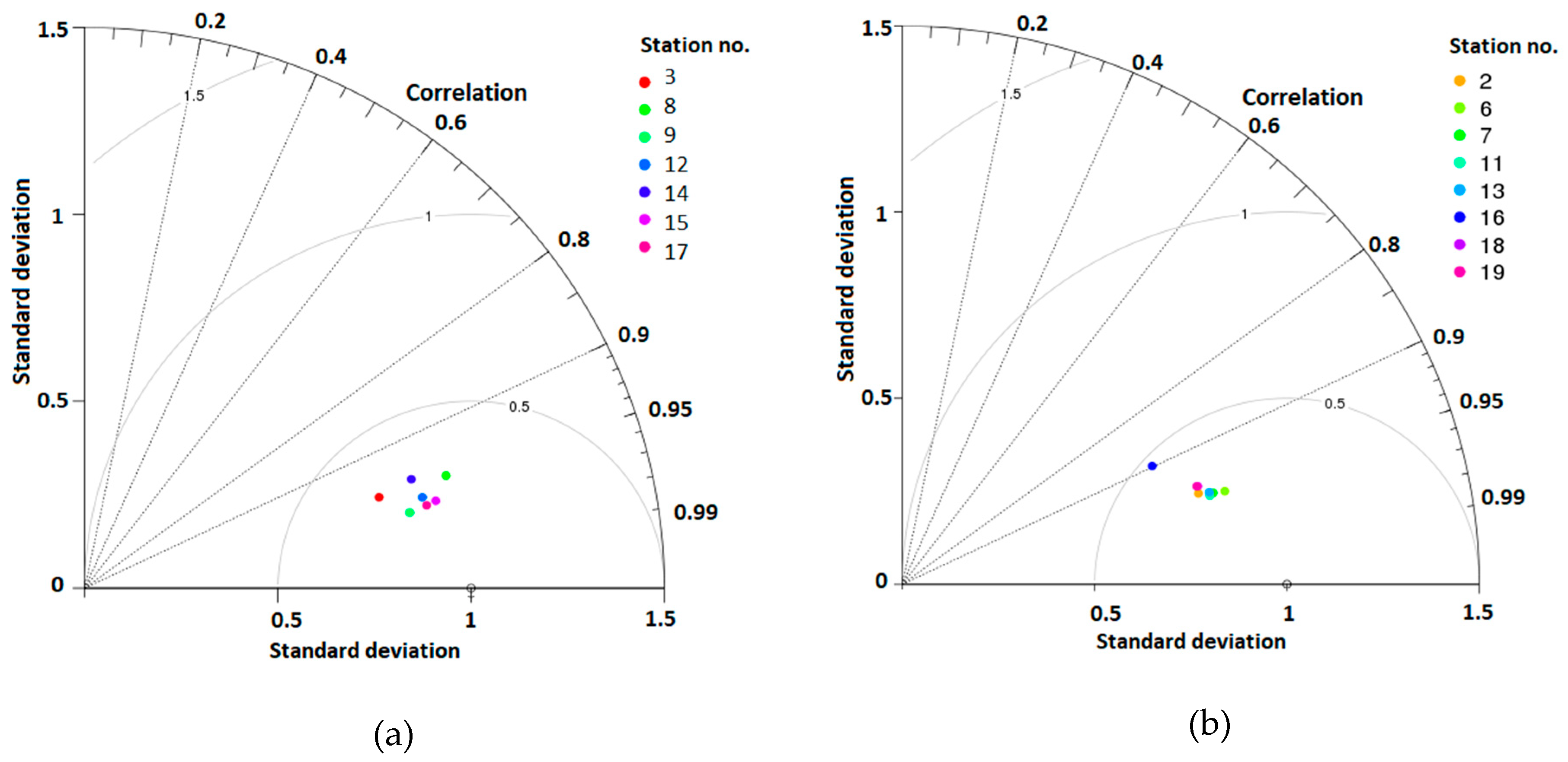
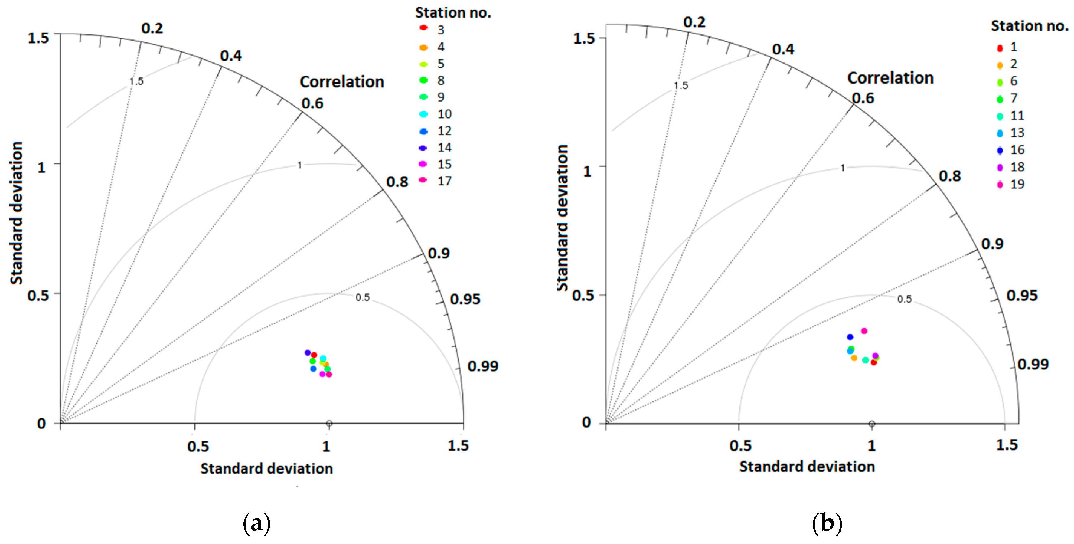
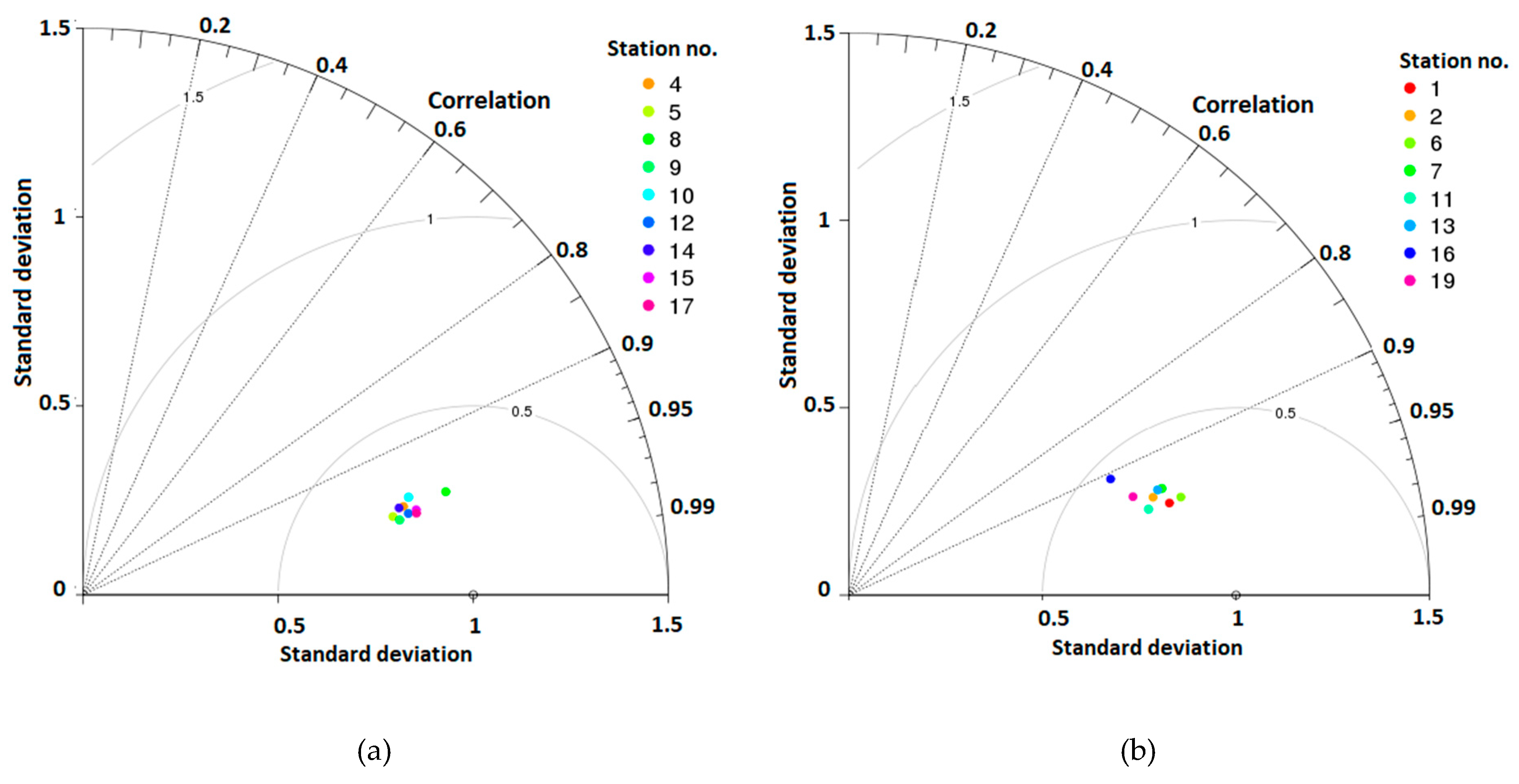
Due to the significant differences in daily temperature ranges between stations located in the valley bottoms and tops, stations were divided into two groups. The value of root mean square error (RMSE), difference (bias), and forecast accuracy were determined on the basis of differences between observation and forecast for each hour and separately for minimum and maximum daily air temperature. Forecast accuracy was calculated for three temperature difference ranges: ±1, ±2, and ±5 °C. The accuracy for a given range specified what percentage of forecast hours were different between forecast and observation below a specified range. In order to make a multifaceted assessment of the quality of the simulation, the results of model verification were graphically presented using a Taylor diagram [31]. This chart allowed us to show three measures commonly used for quality assessment: standard deviation, Pearson’s correlation coefficient, and centered pattern RMS difference.
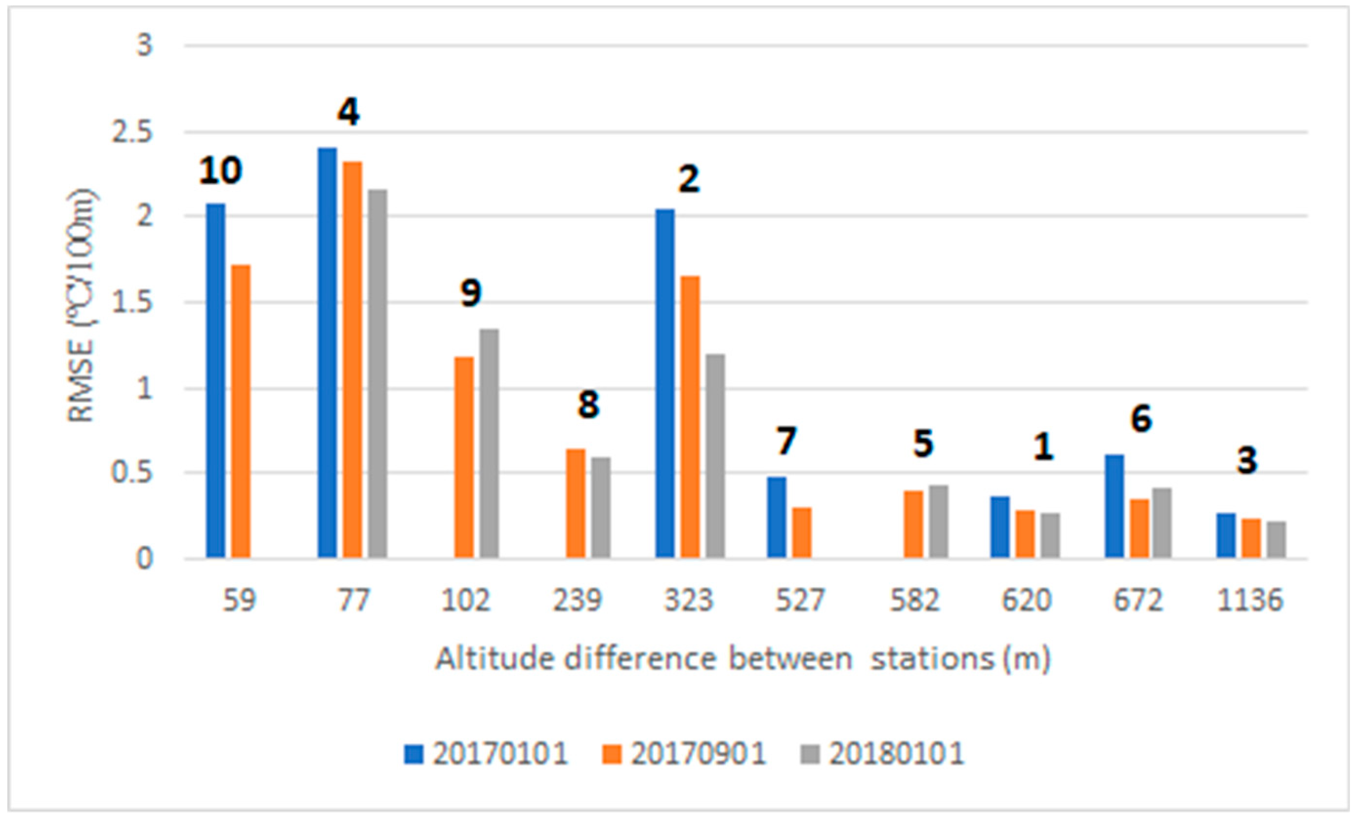
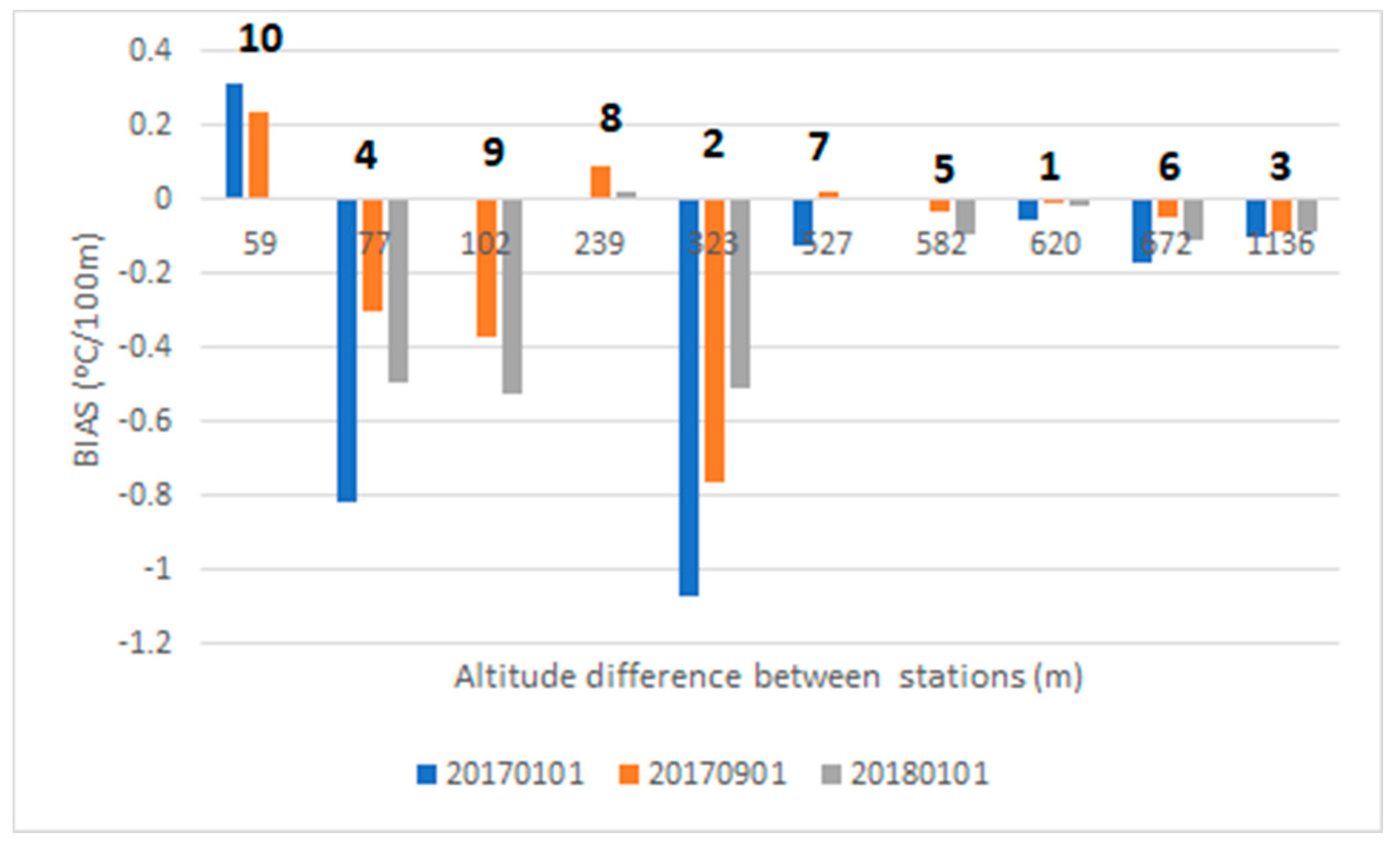
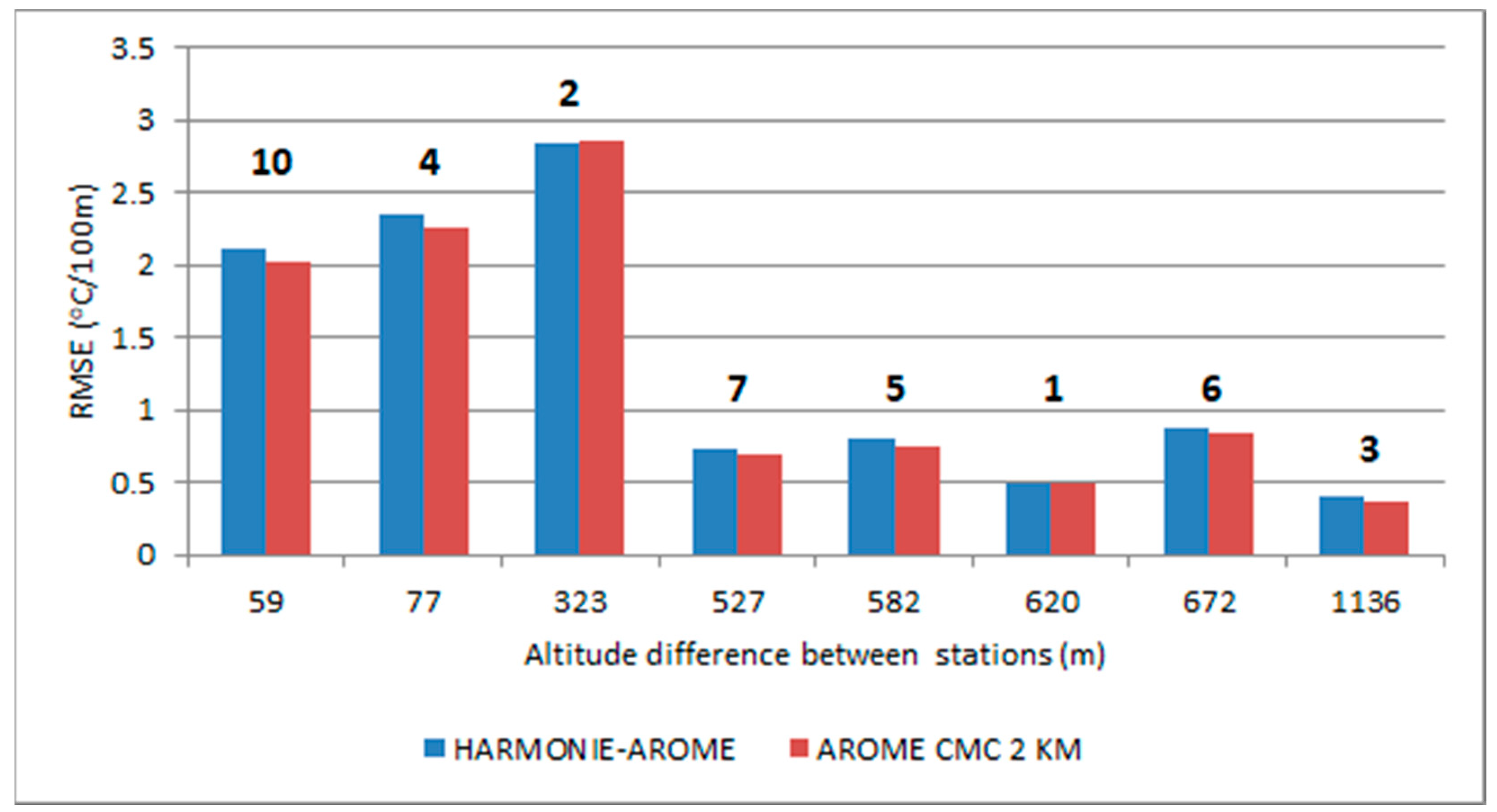
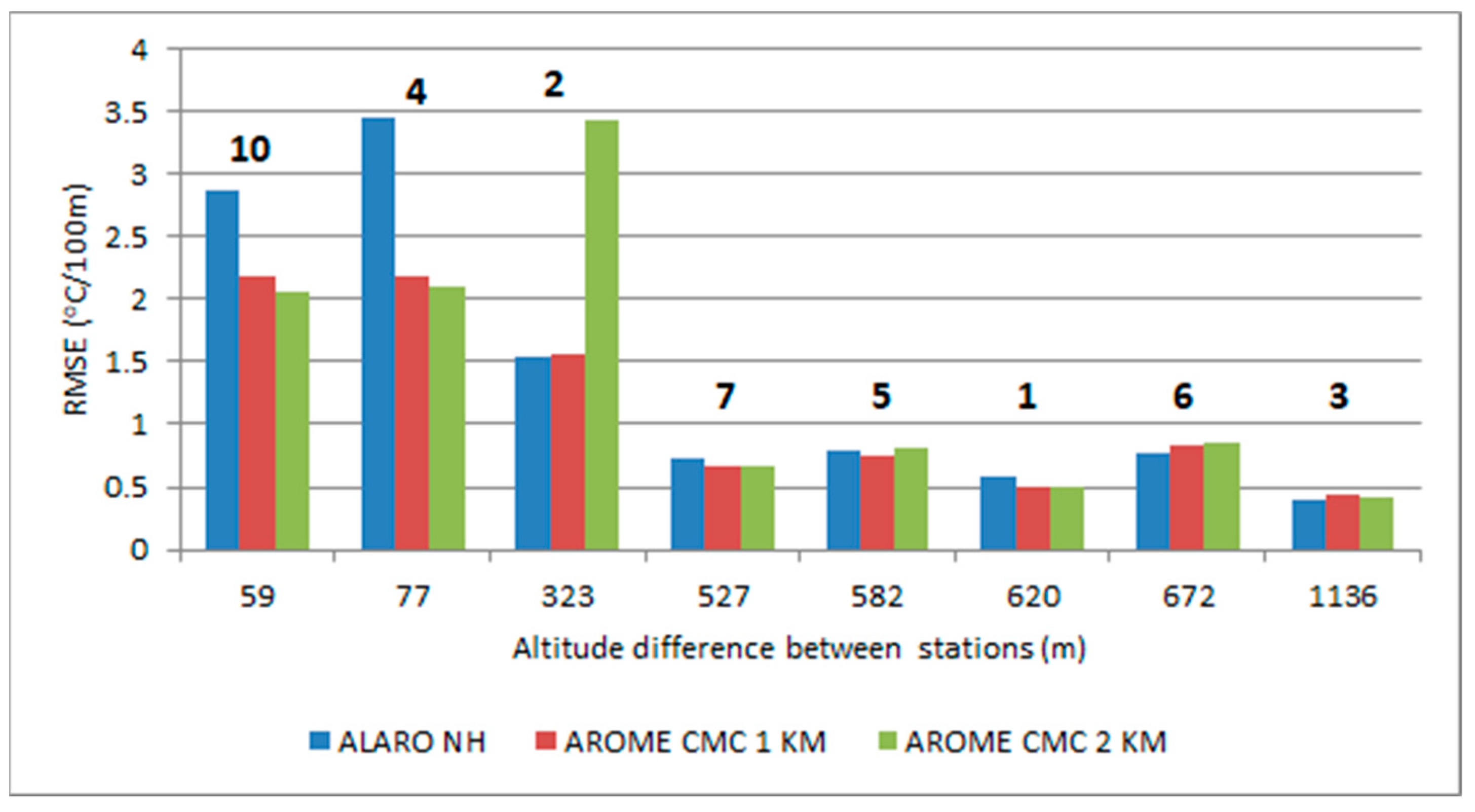
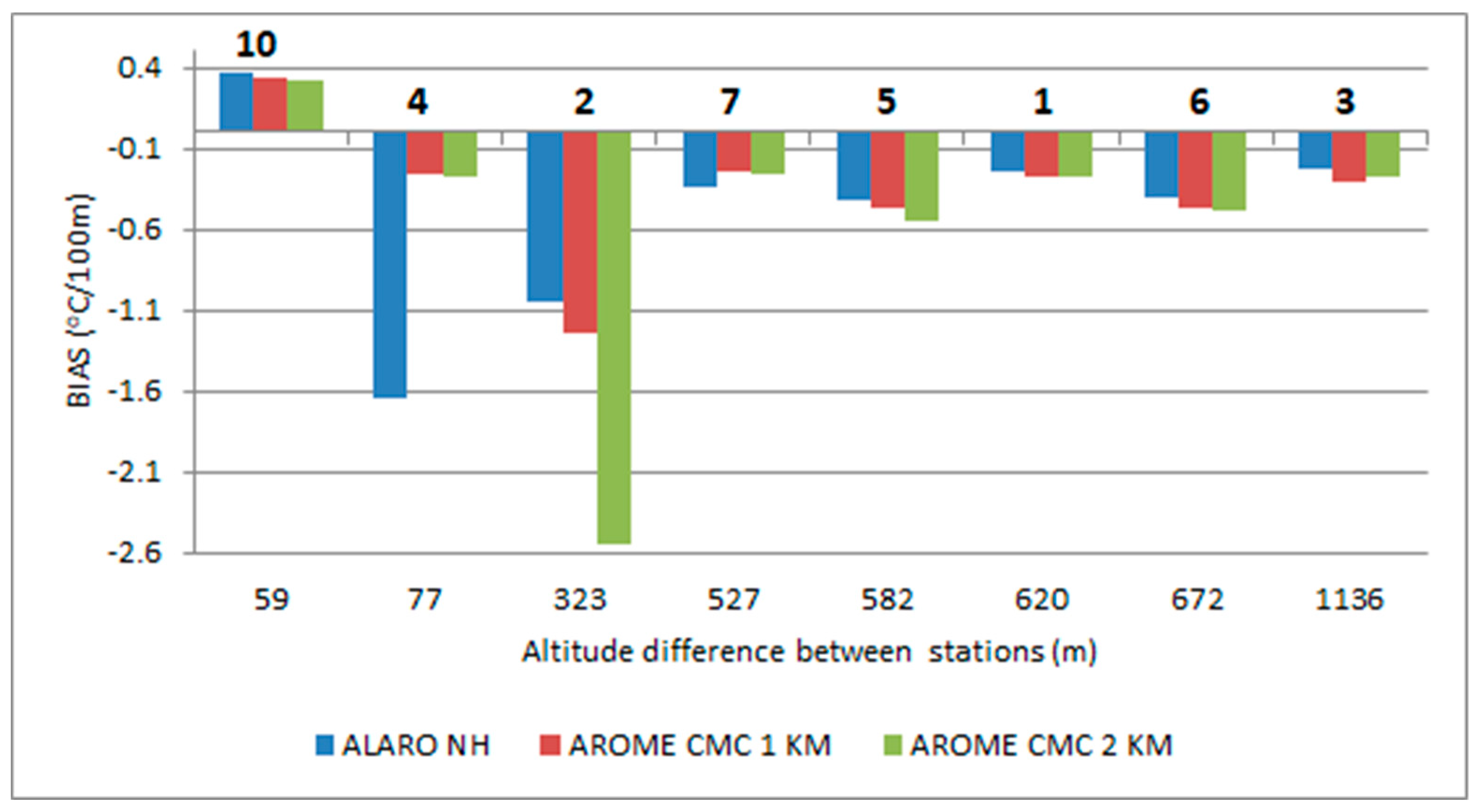
Additionally, for all tested models, predicted vertical temperature gradients were examined for all verified time periods. The value of the vertical temperature gradient determined the state of atmospheric stability, which in turn affected the possibility of smog episodes occurring. Ten pairs of neighboring stations were created to calculate vertical temperature gradients. Detailed information of station pairs for model grids with 1 × 1 km and 2 × 2 km horizontal resolution are presented in Table 6.
The representation of difference in altitude between station pairs in the model domain with 1 × 1 km horizontal resolution was significantly better than that for the model domain with 2 × 2 km resolution (RMSE value for both domains was 55 m for kilometric resolution and 160 m for higher resolution).
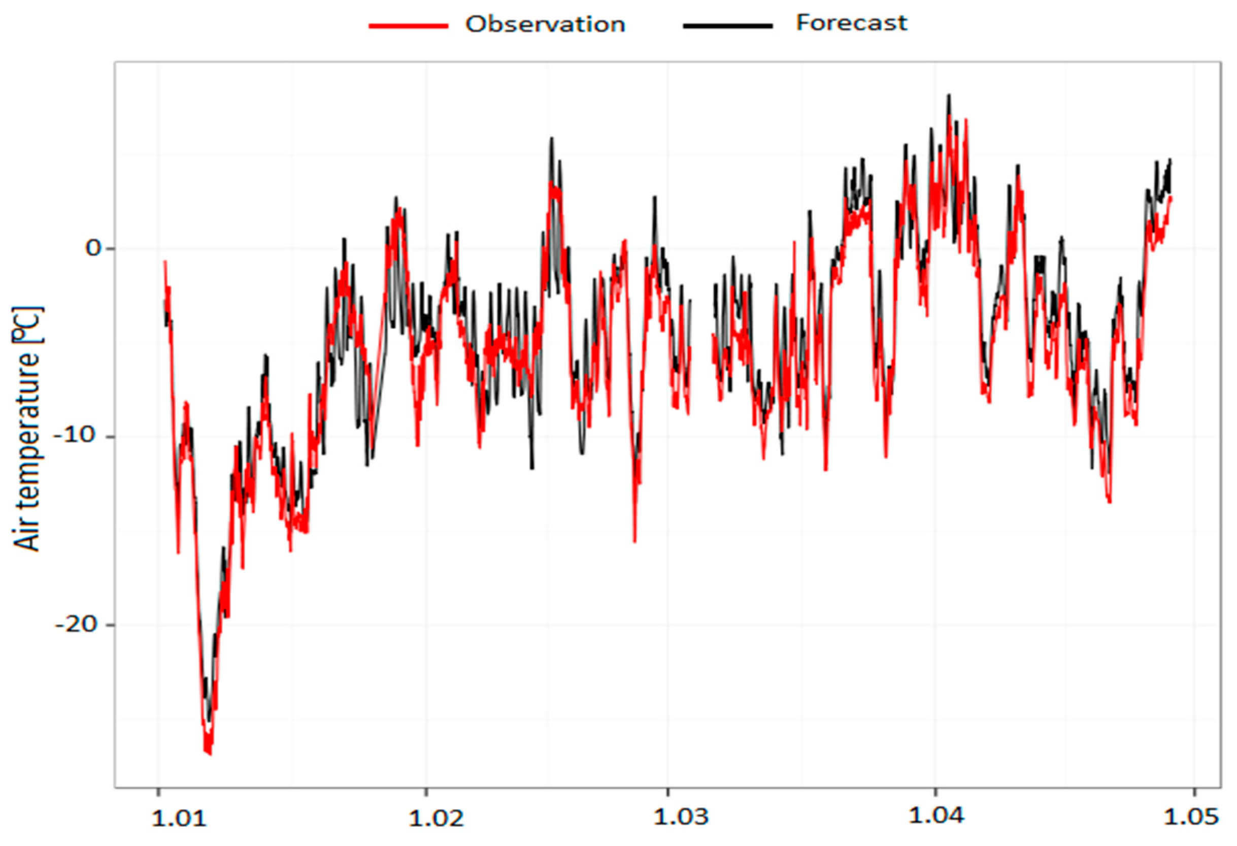
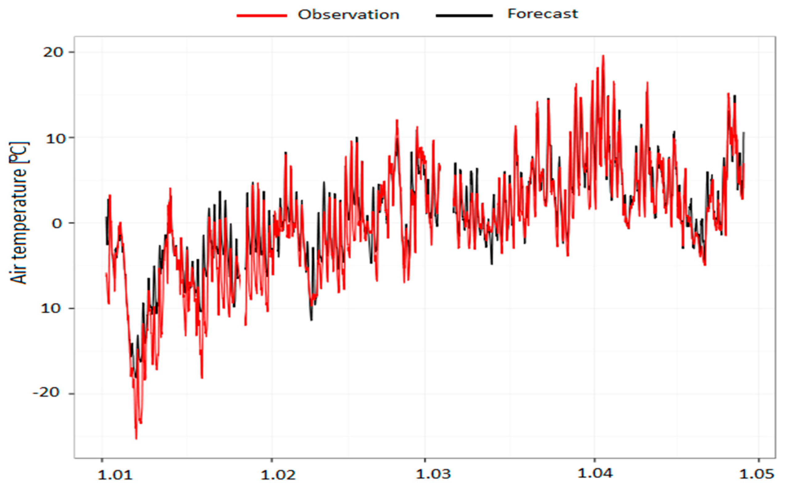
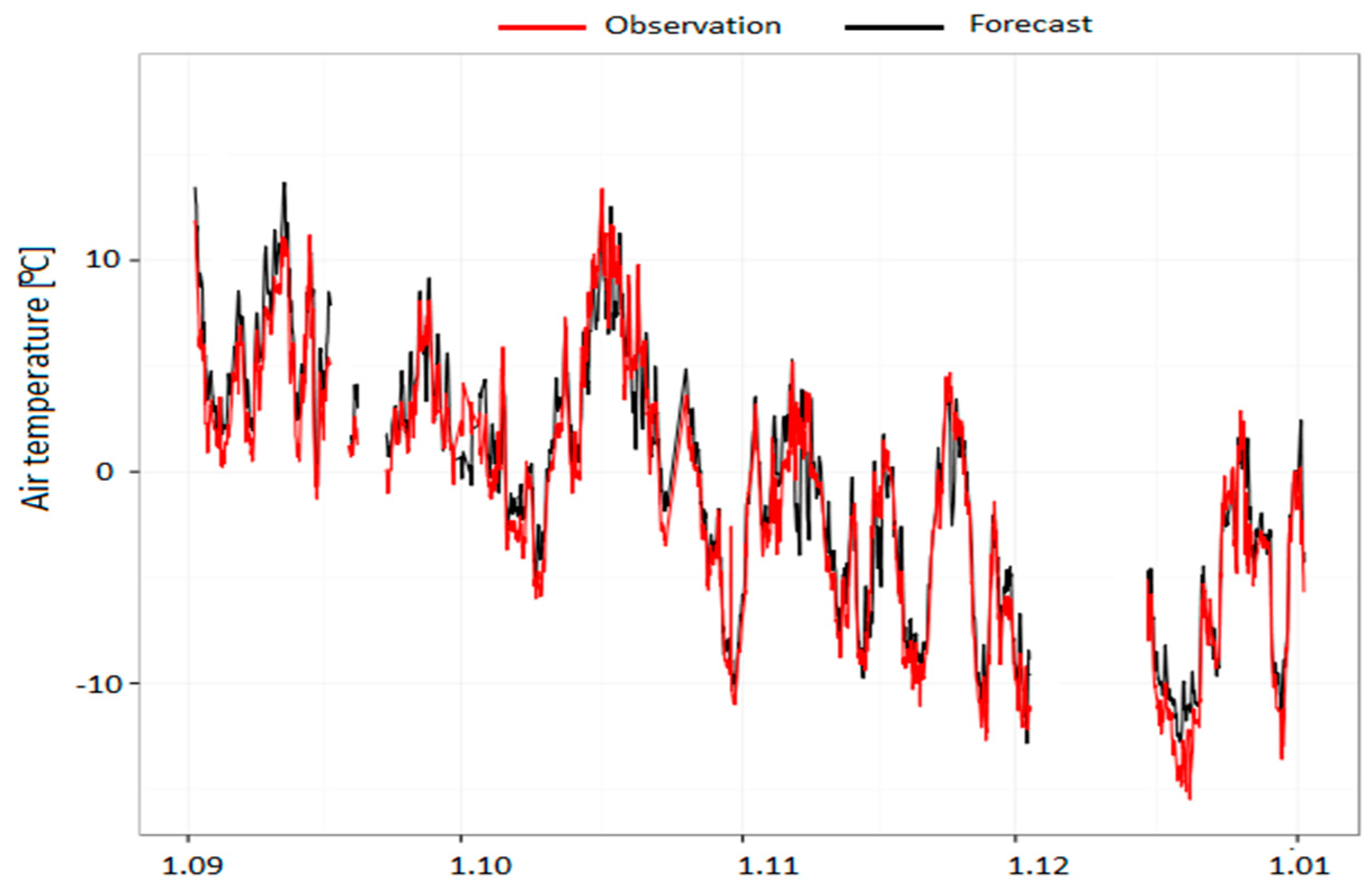
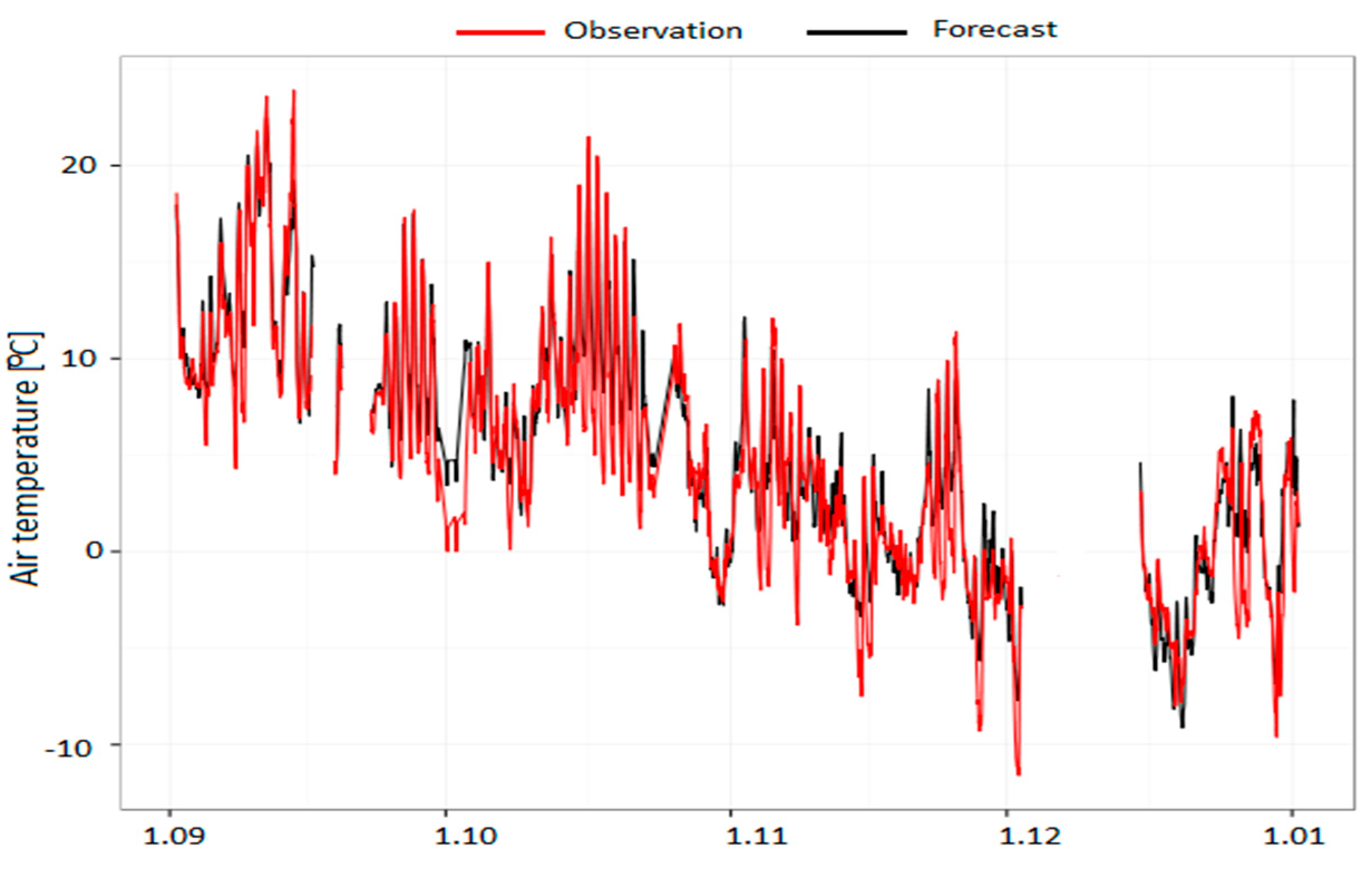
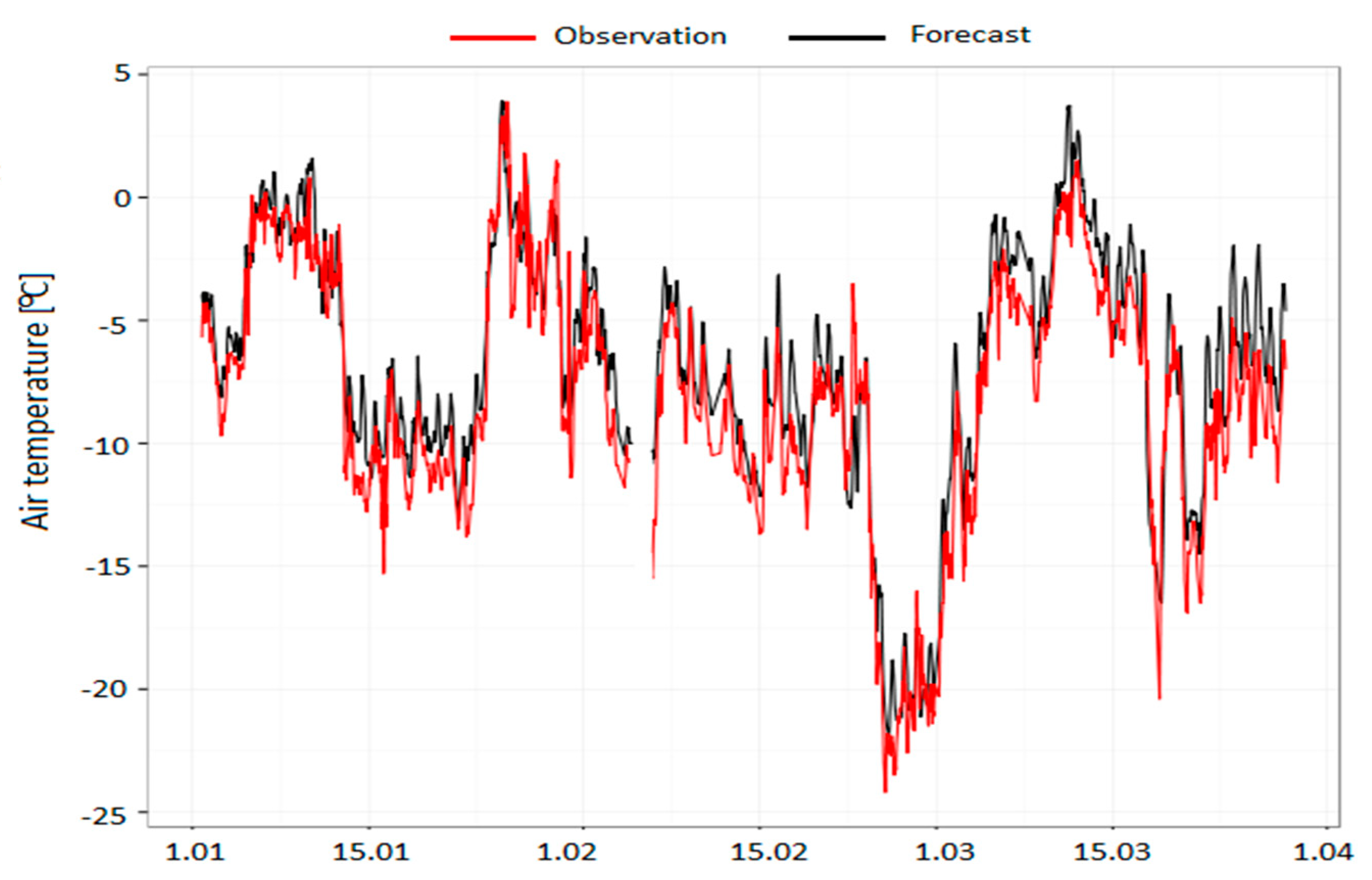
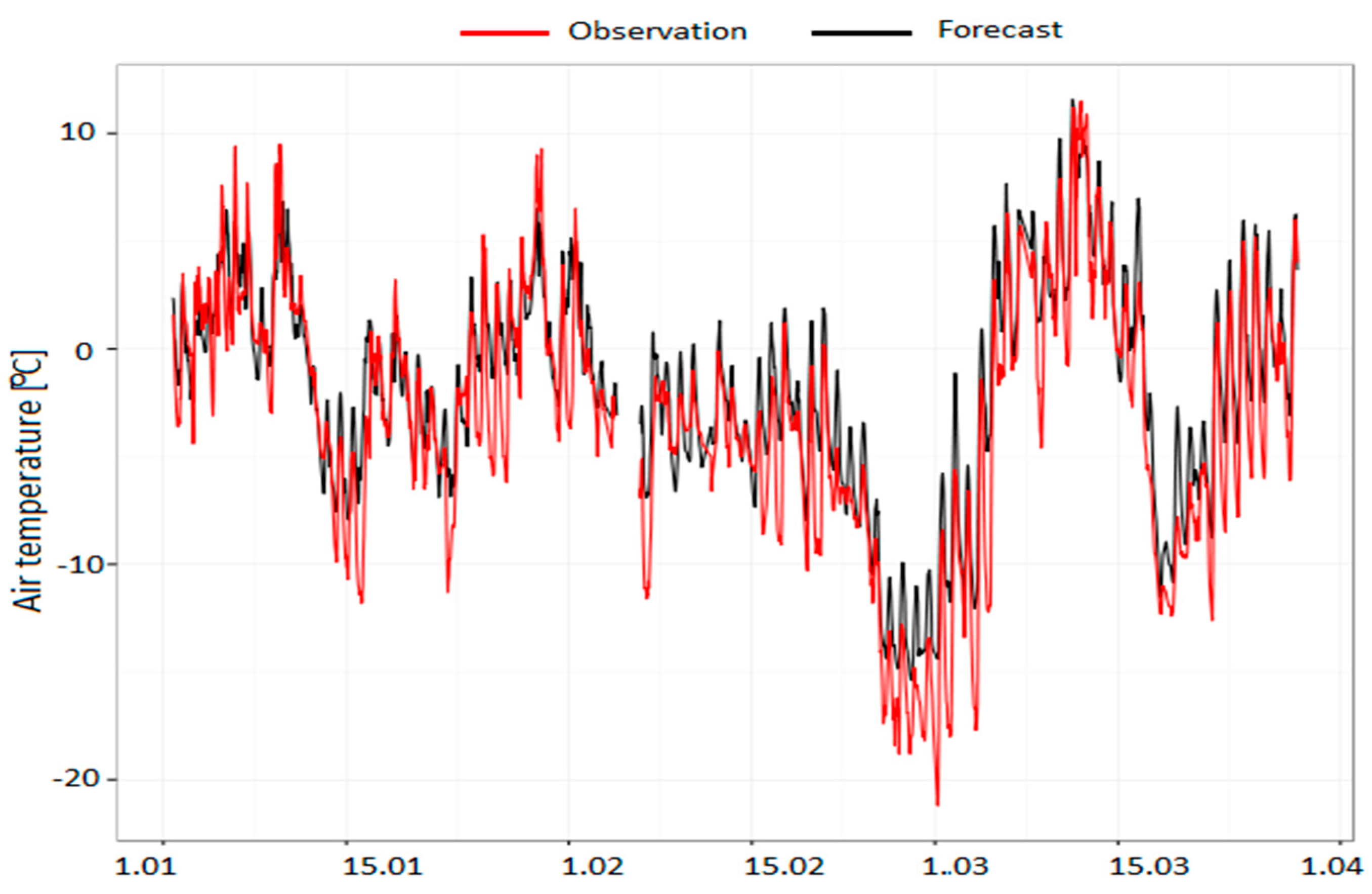
The model performance was also presented as air temperature courses, with 1 h time resolution, separately for the Kasprowy Wierch Mt. (representing hilltops) and Zakopane (representing valleys), for all three subperiods. Both stations were chosen to represent relief variability of the study area because of the large altitude difference between the stations, limited anthropogenic impact on the natural environment, and relatively small differences between actual and model station altitudes. Additionally, as shown in Table 7, Table 8 and Table 9, statistical parameters for both stations were close to the mean values for the whole study area.

3. Results

Our comparison of air temperature forecasts with observations consisted of (i) results of verification of AROME CMC 2 km for three time intervals: winter/spring, 1 January to 30 April 2017 and 1 January to 30 April 2018; and autumn/winter, 1 September to 31 December 2017 (Section 3.1); (ii) a comparison of observations with two limited-area models: AROME CMC 2 km and HARMONIE-AROME, both with resolution of 2 × 2 km, for verification period 1 January to 16 February 2017 (data for 39 days were available) (Section 3.2); and (iii) a comparison of observations with two kilometric scale models, AROME CMC 1 km and ALARO NH, and operational model AROME CMC 2 km. As models differed with length of forecast, only common time periods (6th to 18th forecast hour) were used for verification. The verification period for the two kilometric scale models was 1 January to 16 February 2017, and data for 31 days were available.

3.1. Evaluation of AROME 2 km

During all three subperiods, following the classification of Niedźwiedź [32], atmospheric circulation conditions can be considered as close to the average pattern. That pattern can be characterized with conditions that are controlled mainly by the atmospheric circulation. As shown by Ustrnul [33], in the study area during the cold part of the year, the differences between standard autumn (September to November) and winter (December to February) were negligible, on average. Advection of air masses from the west prevailed, linked to the activity of both cyclonic and anticyclonic centers of atmospheric pressure. During the standard spring (March to May), no synoptic situation type was prevalent (i.e., all types had similar frequency). However, a typical feature for Central Europe is high variability of the circulation patterns from year to year.

3.1.1. Winter/Spring Period, 1 January to 30 April 2017

For the first analyzed period, stations 1 (Wandy Bridge), 4 (Kocmyrzów), 5 (Chorągwica), and 10 (Luboń Wielki) were not included in the analysis because of their significant data gaps.
Results of the comparison representing the first winter/spring period are presented in Table 7. Values of RMSE and bias for the analyzed period, daily values of air temperature extremes, and forecasting accuracy for three ranges of temperature differences were presented separately for stations located in valley bottoms and tops. Mean values of most statistical indicators showed that the forecast of air temperature was better for mountain/hill tops than for valley bottoms. One exception was accuracy with a difference range of ±1 °C, for which the parameters for both groups were comparable (tops, 39.8 ± 6.7 %; valleys, 40.9 ± 2.5 %). Forecast accuracy for ranges ±2 °C and ±5 °C was higher for mountain/hill tops.
Lower forecast accuracy for valley stations (ranges ±2 °C and ±5 °C) was probably caused by underestimation of minimal temperatures in the valleys predicted by the model compared to the mountain/hill tops.
This study points out that RMSE value in some cases is not a sufficient indicator to assess forecast quality. The station with the highest RMSE value (No. 3) had better accuracy in the range ±1 °C compared to selected stations with lower RMSE. Compatibility of diurnal temperature range from the model and from the measurements for stations located at the tops was better than that for stations in the valleys, which was caused by better compatibility of forecast minimum air temperature. Mean values of RMSE minimum daily temperature for stations located at the tops were significantly lower than those for stations in valleys. The difference between RMSE values for minimum and maximum daily air temperature for six out of eight analyzed stations (2, 7, 13, 16, 18, and 19) was greater than one. The maximum difference between RMSE values for minimum and maximum daily temperatures was measured for station 16 (difference of 3.29 °C). The minimum difference between RMSE values for minimum and maximum daily observations was 0.16 °C for mountain station 17. Differences in mean RMSE and bias values for maximum daily air temperature between stations located at tops and in valleys were small. Contrary to top stations, the RMSE values for minimum daily air temperature for all valley stations were higher than the values for maximum daily air temperature. The RMSE values for minimum daily air temperature for three mountain stations were lower than the values for maximum daily air temperature.
Additional information is provided by the Taylor diagram presented in Figure 2. Points representing forecast compliance for valley stations were less spread out than points corresponding to forecast errors for stations located at the tops. This indicated that the forecasts for valley stations for all measurement points were similar, with the exception of station 16, for which the forecast error was much larger. The large spread of points corresponding to stations located at the tops indicated their large diversity.
Time series of air temperature for the valley station at Zakopane and the station at the top of Kasprowy Wierch are presented in Figure 3 and Figure 4.
Based on surface pressure charts prepared by IMWM-NRI, two high-pressure system periods on 7–9 and 27–31 January 2017 over the analyzed area were separated. An analysis of those periods indicated higher error of numerical weather prediction for valley stations compared to hill/mountain top stations. The minimum temperature values for those periods were overestimated by as much as 10 °C, which affected the RMSE value representing the whole analyzed period.

3.1.2. Autumn/Winter Period, 1 September to 31 December 2017

In the second analyzed period, observation data from all stations were used for verification. Results of the comparison representing the autumn/winter period are presented in Table 8. The analyzed period differed significantly from the first winter/spring period. Mean values of all statistical indicators pointed out better compatibility of the forecast for autumn/winter. Mean values of forecast accuracy for three ranges between a group of valleys and tops were comparable. Analyzing values of RMSE and bias separately for hill/mountain tops and valley bottoms, we can conclude that there was no statistically significant difference between the above parameters characterizing both groups. Mean values of RMSE and bias for extreme daily air temperature for stations located at valleys and tops showed that forecast compliance for the maximum temperature was comparable for both groups. More significant differences were seen for daily minimum air temperature: the average RMSE value for stations located at the tops was lower than the value for stations in valleys. The difference between RMSE values for minimum and maximum daily air temperature for three valley stations (7, 16, and 19) was greater than 1 °C. During the previous analyzed period, the difference in RMSE value for extreme daily temperatures was also higher for the stations mentioned above.
Taylor diagrams in Figure 5 for two groups of stations also showed that the quality of air temperature forecast was comparable for all stations. Points representing forecast compliance for stations located at tops were less spread out than points corresponding to forecast error for stations located in valley bottoms. The highest RMSE value for points at top stations was measured for station 10 (Luboń Wielki). The forecast for station 10 also had the lowest accuracy in the range ±1 °C compared to all stations.
Figure 6 and Figure 7 present time series of air temperature for valley station Zakopane and the station at the top of Kasprowy Wierch.
While the diurnal amplitude and synoptic variability of temperature calculated for mountain top stations followed the observations, at the valley station in Zakopane, for two periods (middle of October and second part of November) corresponding to high-pressure system situations, the minimum diurnal temperatures forecast was overestimated compared to the observations.

3.1.3. Winter/Spring Period, 1 January to 30 April 2018

For the last analyzed period, stations 2 and 18 were not included in the analysis because they had significant data gaps. Results of the comparison for stations located in various landforms representing the second winter/spring period are presented in Table 9. Mean RMSE values for all periods and extreme daily values and forecast accuracy for stations located in valleys and at tops were comparable with the values for the first analyzed winter/spring period. The forecast error for the autumn/winter period was significantly lower than for both winter/spring periods. The difference in RMSE values for minimum and maximum daily temperature for five of eight valley stations was greater than 1 °C (stations 2, 7, 13, 16, and 19). Stations mentioned above in the first analyzed period also had a difference in RMSE values greater than 1 °C. The maximum difference of RMSE values for daily extreme temperatures was measured for station 16 (difference of 3.04 °C). Lower RMSE values for minimum daily temperature than for maximum daily temperature for five mountain stations pointed out better compatibility of forecasted minimum than maximum daily temperature for these stations (4, 5, 9, 12, and 14).
Taylor diagrams presented in Figure 8 point out that the forecast results are better for mountain/hill top than valley stations.
Figure 9 and Figure 10 present time series of modeled and measured values of air temperature at 2 m a.g.l. for the stations in Zakopane and at Kasprowy Wierch Mt. As in the previous winter/spring season, the minimum temperatures for valley stations were often overestimated, which was noticeable in the temperature course for the Zakopane station.
In the period between the end of February and the beginning of March 2018, the southern part of Poland was under the influence of Arctic air. The air mass was transformed into a continental one. In parallel, there was an inflow of Arctic air from the east of the continent. At most of the analyzed stations, very low minimum temperatures were measured. The difference between forecast and measured minimum air temperatures for valley stations was as high as 10 °C. Differences between observed and forecast minimum temperatures for stations located at the tops were smaller than for stations in valley bottoms. The analysis of the forecast cloudiness observed for the synoptic stations at Kraków and Zakopane did not show major differences that would significantly affect the reduction of outgoing longwave radiation.
The comparison of all three subperiods presented above showed relatively good agreement between the model data and measurements and a general similarity between the periods distinguished. However, there were some differences in the statistical parameters for stations representing different landforms. For hilltop stations, mean RMSE values for all periods and for minimum daily air temperature showed better agreement between forecast and observations than valley stations. As those features can be found for all three periods, it can be assumed that they were typical for the study area. The largest problem with air temperature prediction in the valleys was related to the influence of high-pressure systems, which was shown using cases of synoptic conditions; a more thorough statistical analysis was not possible because the available sample was too small.

3.1.4. Temperature Gradient Analysis for AROME 2 km

The RMSE values of temperature gradient calculated based on differences between pairs of neighboring stations were analyzed. Since some stations were not included in the analysis for individual time periods (lack of data), some station pairs were also excluded. For the period 1 January to 30 April 2017, stations pairs 5, 8, and 9 were excluded, and for 1 January to 30 April 2018, stations 7 and 10 were excluded. RMSE values for predicted temperature gradients are presented in Figure 11. Figure 11 and Figure 12 show the numbers of station pairs used for temperature gradient analysis.
Obtained RMSE values of temperature gradients were in the range between 0.3 and 2.5 °C/100 m. The highest RMSE values were observed for pairs with the least altitude difference (Figure 11). The bias between observed and predicted gradients by the model had a similar pattern (Figure 12).
It was also noticeable that the temperature gradient predicted by the model was underestimated for most of the station pairs (negative bias values). A possible explanation for such an effect can be uncertainty of station altitude reproduced in the model domain. We can conclude that the prediction of temperature gradient based on station pairs having altitude differences greater than 500 m was fairly accurate (RMSE < 0.5 °C/100 m, bias < 0.1 °C/100 m), thus the possibility of a smog episode can be reliably predicted by the model using such station pairs.

3.2. Comparison of Observations with AROME CMC 2 km and HARMONIE-AROME

In order to improve the quality of numerical prediction for areas with a large diversity of relief, HARMONIE-AROME model tests were performed.
A comparison of observations with two models was performed for the period 1 January to 16 February 2017, which can be evaluated as representative for winter time. According to the calendar of T. Niedźwiedź [33], on 15 days (32% of the days in that period) there were synoptic situations with advection from the west, but no longer periods with the same situation. The advection direction changed every few days. There was a period of a few days with anticyclonic-type atmospheric circulation and no advection, and a smog episode occurred at that time (26–29 January 2017). On 18 days of the period, polar maritime air masses came into the study area, while on 22 days there were polar continental air masses. The period 1 January to 16 February 2017 presented typical conditions of the transitional climate of Central Europe, with large variability of the synoptic situation and frequent changes in advection conditions, which was the reason for frequent changes in weather conditions.
Both models had the same size domain and resolution (2 × 2 km). The verified period was relatively short, therefore only bias and RMSE values were calculated for stations. Data for stations 1, 4, and 5 had many gaps and, therefore, were not included in the analysis. A comparison of observations with models is presented in Table 10. The analysis of RMSE and bias values for the remaining stations, assuming a significance level of 5%, indicated that the differences between the models was statistically insignificant. Stations with the highest and lowest RMSE in both groups (valley bottoms and hill and mountain tops) were the same for both models. The test for the winter period for HARMONIE-AROME pointed out that differences in dynamics and turbulence scheme had no significant impact on improvement of the forecast air temperature at a height of 2 m above ground level compared to the results of AROME CMC 2 km.
Air temperatures from selected stations were used to compare air temperature gradients between pairs of ground stations. For the period 1 January to 16 February 2017, station pairs 8 and 9 were excluded because they had a small amount of data. A comparison of RMSE values for predicted temperature gradients between two models (HARMONIE-AROME and AROME CMC 2 km) presented in Figure 13 pointed out that forecast accuracy for both models was similar.
Bias values for predicted temperature gradients shown in Figure 14 were also comparable between HARMONIE-AROME and AROME CMC 2 km. A significantly higher value for station pair no. 2 was caused by high underestimation of altitude difference between stations (difference in model domain was 50 m, while real altitude difference was 323 m).

3.3. Comparison of Observation with Kilometric Scale Models AROME CMC 1 km, ALARO NH, and AROME CMC 2 km

The previously described test compared the performance of two kilometric scale models to the operational AROME CMC 2 km model used by the Polish group of ALADIN for routine forecast calculation for the analyzed area. If we increase the model resolution and number of vertical levels, we can expect that local dynamic processes like katabatic flow and temperature inversion in the valleys will be better reproduced by the model because of better topography representation, and the denser computational grid can better reproduce small-scale phenomena. For the short winter period, tests of AROME CMC 1 km and ALARO NH (both with 105 vertical levels) were run.
Below are presented the results of the comparison of the AROME CMC 2 km operational model and the two kilometric scale models, AROME CMC and ALARO NH for the period 1 January to 16 February 2017. Data for stations 1, 4, and 5 were not included in the analysis because of many gaps. Table 11 presents the RMSE values and bias error of forecast. RMSE values for all stations were very similar. Despite the fact that AROME CMC 1 km had more vertical levels and better horizontal resolution, differences between the AROME CMC 2 km operational model and the new version were insignificant. Analyzing RMSE values and bias error separately for hill/mountain tops and valley bottoms, we can conclude that differences between models were within the limits of single standard deviation of mean value. The lowest RMSE value for hill/mountain stations was obtained in AROME CMC 1 km, while better forecasting for stations in valley bottoms was obtained by ALARO NH.
Observations of air temperature from selected stations were used for verification of temperature gradients; stations pairs 8 and 9 were excluded because they had a small amount of data. Figure 15, containing plots of RMSE values for predicted temperature gradients, pointed out that for altitude difference greater than 500 m, the differences between kilometric scale models and the model with a bigger resolution were small. There was significantly better forecast compliance for kilometric scale models compared with AROME CMC 2 km for station pair No. 2, which was caused by better representation of altitude difference in the model domain. Predicted air temperature gradients for pairs with altitude differences less than 100 m were similar for AROME CMC 2 km and AROME CMC 1 km.
Figure 16 presents bias values for predicted temperature gradients for three model configurations. Bias for pairs with altitude difference greater than 500 m were comparable, and were slightly underestimated up to −0.6 °C/100 m.

4. Conclusions

One of the aims of this paper was to evaluate the performance of the operational AROME CMC 2 km model, used by IMWM-NRI in the region of the Polish Western Carpathian Mts. The analysis of the results for three time periods (two winter/spring and one autumn/winter) indicates much better compatibility of forecasts for AROME CMC 2 km for hilltop stations than for valley ones. Bigger forecast error is caused by overestimation of the minimum temperatures, particularly visible for stations located in the valley bottoms. The largest differences between forecast and observed minimum temperatures for stations in valleys occurred when the analyzed area was under the influence of strong high-pressure systems. During such synoptic situations, cold air pools often form in the valley bottoms as a result of atmospheric calm or very weak winds and katabatic flows. Therefore, air temperature reaches much lower values than in areas located at a similar altitude but in an open, flat environment. Significant overestimation of the minimum temperature for stations in the valleys indicates errors in the prediction of thermal stratification of atmosphere inside the valleys. The air temperature forecast of AROME CMC 2 km for stations at the tops is better than the forecasts for stations in the valleys. Particularly large differences in forecast error between stations in the valleys and those at the tops occur in the winter season. Despite the problems with forecasting minimum temperatures in the valleys, it has been demonstrated that based on temperature gradients calculated on the basis of station pairs having an altitude difference greater than 500 m, it is possible to reliably predict thermal inversions leading to the formation of smog episodes in the valleys.
The second aim of the paper was to verify the hypothesis that in mountain areas, the increased resolution of the ALADIN-HIRLAM NWP system would significantly improve the accuracy of the air temperature forecast at 2 m above the ground. A comparison of the results of the AROME CMC 2 km operational model with the HARMONIE-AROME model, which uses other turbulence and dynamics, showed no significant improvement in forecast air temperature for stations at the tops and in the valleys. A comparison of the results of the AROME CMC 2 km operating model with a resolution of 1 × 1 km and more vertical levels (105) did not show significant improvement in forecast temperature as well. One possible reason could be that there were still not enough vertical levels representing air masses in the valleys. It can be improved by redistributing the lowest model levels in future studies. Accurate representation of the vertical profiles of atmosphere is strongly dependent on the amount and location of vertical levels. However, previous studies pointed out that a more important factor for properly forecasting the spatial variability of air temperature in areas with variable topography is horizontal resolution rather than vertical [34,35]
Further works should be aimed at comparing other meteorological parameters affecting thermal stratification in valleys and conducting a deeper analysis of modelling systems to identify the parameters and physical processes affecting the quality of thermal stratification forecasts for areas with complex topography. Analysis of forecasted temperature gradients calculated using pairs of hilltop/valley stations points out that for pairs with an altitude difference greater than 500 m, the temperature gradient prediction is significantly better (RMSE < 0.5 °C/100 m, bias < 0.1 °C/100 m) compared to pairs with a smaller altitude difference.

Author Contributions

The experiment was conceptualized by P.S., A.B., B.B., and M.Z.; Methodology, A.B., B.B., and M.Z.; software, P.S., B.B.; validation, P.S.; formal analysis, P.S., A.B., and M.Z.; investigation, P.S., B.B., and M.Z.; resources, all coauthors; data curation, P.S., A.B., and B.B.; writing—original draft preparation, all coauthors; writing—review and editing, all coauthors; visualization, P.S.; supervision, A.B., B.B., and M.Z.; project administration, P.S.

Funding

This research was partly funded by the EU Project POWR.03.02.00-00-I004/16 (PS) and Ministry of Science and Higher Education subsidy, project no. 16.16.220.842-B02. This research has been partly supported by IMWM-NRI, grant number DS.-M10/2018.

Acknowledgments

We are grateful to both anonymous reviewers for their detailed and constructive comments on the content of the manuscript. The comments allowed us to improve significantly the overall quality of the manuscript.

Conflicts of Interest

The authors declare no conflict of interest.

Appendix A

Table A1. Height of lowest model levels up to 3 km altitude for 60 and 105 vertical levels used in forecast.
105 Vertical Levels60 Vertical Levels
Number of Vertical LevelHeight of Vertical Level (km a.g.l.)Number of Vertical LevelHeight of Vertical Level (km a.g.l.)
10.00910.01
20.02920.035
30.05130.072
40.07540.124
50.150.196
60.12960.289
70.1670.405
80.19480.546
90.23290.714
100.273100.91
110.318111.134
120.367121.387
130.42131.67
140.479141.983
150.542152.327
160.611162.701
170.686173.105
180.767
190.855
200.951
211.054
221.166
231.285
241.414
251.552
261.7
271.857
282.025
292.202
302.39
312.588
322.796
333.014

References

  1. Serafin, S.; Adler, B.; Cuxart, J.; Wekker, S.; Gohm, A.; Grisogono, B.; Kalthoff, N.; Kirshbaum, D.; Rotach, M.; Schmidli, J.; et al. Exchange Processes in the Atmospheric Boundary Layer Over Mountainous Terrain. Atmosphere 2018, 9, 102. Available online: https://www.mdpi.com/2073-4433/9/3/102 (accessed on 15 March 2019). [CrossRef]
  2. Termonia, P.; Fischer, C.; Bazile, E.; Bouyssel, F.; Brožková, R.; Bénard, P.; Bochenek, B.; Degrauwe, D.; Derková, M.; Khatib, R.; et al. The ALADIN System and its Canonical Model Configurations of cycles CY40T1 and CY41T1. Geosci. Model Dev. 2018, 11, 257–281. Available online: https://www.geosci-model-dev.net/11/257/2018/gmd-11-257-2018.pdf (accessed on 15 March 2019). [CrossRef]
  3. Bengtsson, L.; Andrae, U.; Aspelien, T.; Batrak, Y.; Calvo, J.; Rooy, W.; Gleeson, E.; Hansen-Sass, B.; Homleid, M.; Hortal, M.; et al. The HARMONIE–AROME Model Configuration in the ALADIN–HIRLAM NWP System. AMS 2017, 145, 1919. Available online: https://journals.ametsoc.org/doi/full/10.1175/MWR-D-16-0417.1 (accessed on 15 March 2019). [CrossRef]
  4. Brousseau, P.; Seity, Y.; Ricard, D.; Leger, J. Improvement of the forecast of convective activity from the AROME-France system. Q. J. R. Meteorol. Soc. 2016, 142, 2231–2243. Available online: https://rmets.onlinelibrary.wiley.com/doi/abs/10.1002/qj.2822 (accessed on 15 March 2019). [CrossRef]
  5. Hagelin, S.; Auger, L.; Brovelli, P.; Dupont, O. Nowcasting with the AROME Model: First Results from the High-Resolution AROME Airport. AMS 2014, 29, 773–787. Available online: https://journals.ametsoc.org/doi/full/10.1175/WAF-D-13-00083.1 (accessed on 15 March 2019). [CrossRef]
  6. Yang, X. Configuration of sub-km Harmonie-nowcasting ensemble, Geophysical Research Abstracts. In Proceedings of the EGU General Assembly, EGU 2018, Vienna, Austria, 4–13 April 2018; EGU2018-16337. Available online: https://meetingorganizer.copernicus.org/EGU2018/EGU2018-16337.pdf (accessed on 15 March 2019).
  7. Amodei, M.; Sanchez, I.; Stein, J. Verification of the French operational high-resolution model AROME with the regional Brier probability score. Meteorol. Appl. 2015, 22, 731–745. Available online: https://rmets.onlinelibrary.wiley.com/doi/10.1002/met.1510 (accessed on 15 March 2019). [CrossRef] [Green Version]
  8. Czarnecka, M.; Nidzgorska-Lencewicz, J. Impact of weather conditions on winter and summer air quality. Int. Agrophys. 2011, 25, 7–12. Available online: http://www.old.international-agrophysics.org/en/issues.html?stan=detail&vol=25&numer=1&paper=900&i=2 (accessed on 15 March 2019).
  9. Bokwa, A.; Wypych, A.; Ustrnul, Z. Climate Changes in the Vertical Zones of the Polish Carpathians in the Last 50 Years. In The Carpathians: Integrating Nature and Society Towards Sustainability, Environmental Science and Engineering; Kozak, J., Ed.; Springer-Verlag: Heidelberg/Berlin, Germany, 2013; pp. 89–110. Available online: https://link.springer.com/chapter/10.1007/978-3-642-12725-0_8 (accessed on 15 March 2019).
  10. Wypych, A.; Ustrnul, Z.; Schmatz, D.R. Long-term variability of air temperature and precipitation conditions in the Polish Carpathians. J. Mt. Sci. 2018, 15, 237–253. Available online: https://link.springer.com/article/10.1007/s11629-017-4374-3 (accessed on 15 March 2019). [CrossRef]
  11. Hess, M. Piętra klimatyczne w polskich Karpatach Zachodnich. Zesz. Nauk. UJ Pr. Geogr. 1965, 105, 11. [Google Scholar]
  12. Ustrnul, Z. Influence of foehn winds on air-temperature and humidity in the Polish Carpathians. Theor. Appl. Climatol. 1992, 45, 43–47. Available online: https://link.springer.com/article/10.1007/BF00865992 (accessed on 15 March 2019). [CrossRef]
  13. Dąbrowska, K.; Guzik, M. Atlas of the Tatra Mountains—Abiotic Nature; Tatrzański Park Narodowy: Zakopane, Poland, 2015. [Google Scholar]
  14. Ustrnul, Z.; Wypych, A.; Henek, E.; Czekierda, D.; Walawender, J.; Kubacka, D.; Pyrc, R.; Czernecki, B. Meteorlogical Hazard Atlas of Poland; Instytut Meteorologii i Gospodarki Wodnej & Wydawnictwo Attyka: Kraków, Poland, 2014. [Google Scholar]
  15. Niedźwiedź, T. Temperatura i wilgotność powietrza w warunkach rzeźby pogórskiej Karpat (na przykładzie doliny Raby koło Gaika-Brzezowej). Zesz. Nauk. UJ Pr. Geogr. 1973, 32, 7–88. [Google Scholar]
  16. Oke, T.R. Initial Guidance to Obtain Representative Meteorological Observations at Urban Sites; WMO Report No. 81, WMO/TD No. 1250; WMO: Geneva, Switzerland, 2004; Available online: https://library.wmo.int/pmb_ged/wmo-td_1250.pdf (accessed on 15 March 2019).
  17. Bokwa, A.; Hajto, M.J.; Walawender, J.P.; Szymanowski, M. Influence of diversified relief on the urban heat island in the city of Kraków, Poland. Theor. Appl. Climatol. 2015, 122, 365–382. Available online: https://link.springer.com/article/10.1007/s00704-015-1577-9 (accessed on 15 March 2019). [CrossRef] [Green Version]
  18. Szczęch-Gajewska, M.; Bochenek, B.; Kolonko, M.; Jerczyński, M.; Woyciechowska, J.; Sekula, P. ALADIN in Poland. In Proceedings of the 39th EWGLAM and 24rd SRNWP Meeting, Reading, UK, 2–5 October 2017; Available online: http://srnwp.met.hu/Annual_Meetings/2017/download/monday/posters/poster-EWGLAM2017.pdf (accessed on 15 March 2019).
  19. Chambon, P.; Meunier, L.; Guillaume, F.; Piriou, J.; Roca, R.; Mahfouf, J. Investigating the impact of the water-vapour sounding observations from SAPHIR on board Megha-Tropiques for the ARPEGE global model. Q. J. R. Meteorol. Soc. 2015, 141, 1769–1779. Available online: https://rmets.onlinelibrary.wiley.com/doi/full/10.1002/qj.2478 (accessed on 15 March 2019). [CrossRef]
  20. Bénard, P.; Vivoda, J.; Mašek, J.; Smolíková, P.; Yessad, K.; Smith, C.; Brožková, R.; Geleyn, J.-F. Dynamical kernel of the Aladin-NH spectral limited-area model: Revised formulation and sensitivity experiments. Q. J. R. Meteor. Soc. 2010, 136, 155–169. Available online: https://rmets.onlinelibrary.wiley.com/doi/abs/10.1002/qj.522 (accessed on 15 March 2019). [CrossRef] [Green Version]
  21. Hortal, M. The development and testing of a new two-timelevel semi-Lagrangian scheme (SETTLS) in the ECMWF forecast model. Q. J. R. Meteor. Soc. 2002, 128, 1671–1687. Available online: https://rmets.onlinelibrary.wiley.com/doi/10.1002/qj.200212858314 (accessed on 15 March 2019). [CrossRef]
  22. Cuxart, J.; Bougeault, P.; Redelsberger, J.-L. A turbulence scheme allowing for mesoscale and large-eddy simulations. Q. J. R. Meteor. Soc. 2000, 126, 1–30. Available online: https://rmets.onlinelibrary.wiley.com/doi/10.1002/qj.49712656202 (accessed on 15 March 2019). [CrossRef]
  23. Bougeault, P.; Lacarrere, P. Parameterization of orography induced turbulence in a meso-beta-scale model. Mon. Weather Rev. 1989, 117, pp. 1870–1888. Available online: https://journals.ametsoc.org/doi/abs/10.1175/1520-0493%281989%29117%3C1872%3APOOITI%3E2.0.CO%3B2 (accessed on 15 March 2019).
  24. Masson, V.; Seity, Y. Including atmospheric layers in vegetation and urban offline surface schemes. J. Appl. Meteorol. Climatol. 2009, 48, 1377–1397. Available online: https://journals.ametsoc.org/doi/10.1175/2009JAMC1866.1 (accessed on 15 March 2019). [CrossRef]
  25. Müller, M.; Homleid, M.; Ivarsson, K.I.; Køltzow, M.A.; Lindskog, M.; Midtbø, K.H.; Andrae, U.; Aspelien, T.; Berggren, L.; Bjørge, D. AROME-MetCoOp: A Nordic convective-scale operational weather prediction model. Weather Forecast. 2017, 32, 609–627. Available online: https://journals.ametsoc.org/doi/full/10.1175/WAF-D-16-0099.1 (accessed on 15 March 2019). [CrossRef]
  26. Nielsen, K.P.; Gleeson, E.; Rontu, L. Radiation sensitivity tests of the HARMONIE 37h1 NWP model. Geosci. Model Dev. 2014, 7, 1433–1449. Available online: https://www.geosci-model-dev.net/7/1433/2014/gmd-7-1433-2014.html (accessed on 15 March 2019). [CrossRef] [Green Version]
  27. Masson, V.; Le Moigne, P.; Martin, E.; Faroux, S.; Alias, A.; Alkama, R.; Belamari, S.; Barbu, A.; Boone, A.; Bouyssel, F.; et al. The SURFEXv7.2 land and ocean surface platform for coupled or offline simulation of earth surface variables and fluxes. Geosci. Model Dev. 2013, 6, 929–960. Available online: https://www.geosci-model-dev.net/6/929/2013/ (accessed on 15 March 2019). [CrossRef] [Green Version]
  28. Gerard, L.; Piriou, J.-M.; Brožková, R.; Geleyn, J.-F.; Banciu, D. Cloud and precipitation parameterization in a meso-gammascale operational weather prediction model. Mon. Weather Rev. 2009, 137, 3960–3977. Available online: https://journals.ametsoc.org/doi/full/10.1175/2009MWR2750.1 (accessed on 15 March 2019). [CrossRef]
  29. Lopez, P. Implementation and validation of a new prognostic large-scale cloud and precipitation scheme for climate and data assimilation purposes. Q. J. R. Meteor. Soc. 2002, 128, 229–257. Available online: https://rmets.onlinelibrary.wiley.com/doi/pdf/10.1256/00359000260498879 (accessed on 25 March 2019). [CrossRef]
  30. Pergaud, J.; Masson, V.; Malardel, S.; Couvreux, F. A parameterization of dry thermals and shallow cumuli for mesoscale numerical weather prediction. Bound.-Lay. Meteorol. 2009, 132, 83–106. Available online: https://www.umr-cnrm.fr/IMG/pdf/pergaud_etal_2009.pdf (accessed on 15 March 2019). [CrossRef]
  31. Taylor, K.E. Summarizing multiple aspects of model performance in a single diagram. J. Geophys. Res. 2001, 106, 7183–7192. Available online: https://agupubs.onlinelibrary.wiley.com/doi/abs/10.1029/2000JD900719 (accessed on 15 March 2019). [CrossRef] [Green Version]
  32. Niedźwiedź, T. Kalendarz Typów Cyrkulacji Atmosfery Dla Polski południowej [Calendar of Atmospheric Circulation Types for Southern Poland]; Silesia University, Chair of Climatology: Sosnowiec, Poland, 2018; a computer file; Available online: http://www.kk.wnoz.us.edu.pl/nauka/kalendarz-typow-cyrkulacji/ (accessed on 15 March 2019).
  33. Ustrnul, Z. Warunki Cyrkulacyjne [Atmospheric Circulation Conditions]. In Klimat Krakowa w XX w. [Climate of Kraków in the 20th Century]; Matuszko, D., Ed.; Institute of Geography and Spatial Management, Jagiellonian University: Kraków, Poland, 2007; pp. 21–40, (in Polish with English summary); ISBN 978-83-88424-28-1. Available online: https://denali.geo.uj.edu.pl/publikacje.php?id=000112 (accessed on 25 March 2019).
  34. Billings, B.; Grubišic’, V.; Borys, R. Maintenance of a Mountain Valley Cold Pool: A Numerical Study. AMS 2006, 134, 2266–2278. Available online: https://journals.ametsoc.org/doi/10.1175/MWR3180.1 (accessed on 15 March 2019). [CrossRef]
  35. Chen, Y.; Ludwig, F.; Street, R. Stably Stratified Flows near a Notched Transverse Ridge across the Salt Lake Valley. AMS 2004, 43, 1308–1328. Available online: https://journals.ametsoc.org/doi/pdf/10.1175/1520-0450%282004%29043%3C1308%3ASSFNAN%3E2.0.CO%3B2 (accessed on 15 March 2019). [CrossRef]
Figure 1. (a) Altitude (m a.s.l.) within the domain of ALARO-NH and AROME CMC 1 km models with 1 km × 1 km resolution, and (b) locations of meteorological stations/measurement points on the background of orography map for 1 km × 1 km domain of AROME CMC 1 km and ALARO NH models. Analyzed area is marked with a black frame. Explanation of the letters in Fig. 1a can be found in the text of the Section 2.1. Numbers in fig. 1b as in Table 1.
Atmosphere 10 00186 g001
Figure 2. Taylor diagram for forecast air temperature for (a) mountain and hill peaks and (b) valley bottoms for the period 1 January to 30 April 2017.
Atmosphere 10 00186 g002
Figure 3. Measured and modeled values of air temperature (2 m above the ground) at Kasprowy Wierch station for the period 1 January to 30 April 2017 for AROME CMC 2 km.
Atmosphere 10 00186 g003
Figure 4. Measured and modeled values of air temperature (2 m above the ground) at Zakopane station for the period 1 January to 30 April 2017 for AROME CMC 2 km.
Atmosphere 10 00186 g004
Figure 5. Taylor diagram for forecast air temperature for (a) mountain and hill peaks and (b) valley bottoms for the period 1 September to 31 December 2017.
Atmosphere 10 00186 g005
Figure 6. Measured and modeled values of air temperature (2 m above the ground) at Kasprowy Wierch station for the period 01 September to 31 December 2017 for AROME CMC 2 km.
Atmosphere 10 00186 g006
Figure 7. Measured and modeled values of air temperature (2 m above the ground) at Zakopane station for the period 01 September to 31 December 2017 for AROME CMC 2 km.
Atmosphere 10 00186 g007
Figure 8. Taylor diagram for forecast air temperature for (a) mountain and hill peaks and (b) valley bottoms for the period 1 January to 30 April 2018.
Atmosphere 10 00186 g008
Figure 9. Measured and modeled values of air temperature (2 m above the ground) at Kasprowy Wierch station for the period 1 January to 30 April 2018 for AROME CMC 2 km.
Atmosphere 10 00186 g009
Figure 10. Measured and modeled values of air temperature (2 m above the ground) at Zakopane station for the period 1 January to 30 April 2018 for AROME CMC 2 km.
Atmosphere 10 00186 g010
Figure 11. RMSE values for predicted temperature gradients for three analyzed periods.
Atmosphere 10 00186 g011
Figure 12. Bias values for predicted temperature gradients for three analyzed periods.
Atmosphere 10 00186 g012
Figure 13. RMSE values for predicted temperature gradients for HARMONIE-AROME and AROME CMC 2 km.
Atmosphere 10 00186 g013
Figure 14. Bias values for predicted temperature gradients for HARMONIE-AROME and AROME CMC 2 km.
Atmosphere 10 00186 g014
Figure 15. RMSE values for predicted temperature gradients for two kilometric scale resolution models (AROME CMC 1 km and ALARO NH) and operational AROME CMC 2 km as reference.
Atmosphere 10 00186 g015
Figure 16. Bias values for predicted temperature gradients for two kilometric scale resolution models (AROME CMC 1 km and ALARO NH) and operational AROME CMC 2 km as reference.
Atmosphere 10 00186 g016
Table 1. Meteorological stations/measurement points used in the study. JU, Jagiellonian University; IMWM-NRI, Institute of Meteorology and Water Management, National Research Institute.
No.NameLatitudeLongitudeAltitude (m a.s.l.)Manager of the StationLand Form
1Wandy Bridge50.05320.049197JUValley bottom
2Jeziorzany49.99619.775211JUValley bottom
3Garlica Murowana50.14219.931270JUHill top
4Kocmyrzów50.14320.132299JUHill top
5Chorągwica49.95920.083436JUHill top
6Balice50.08319.8237IMWM-NRIValley bottom
7Zakopane49.29419.96855IMWM-NRIValley bottom
8Kasprowy Wierch49.23319.9821991IMWM-NRIMountain top
9Libertow49.97319.895314IMWM-NRIHill top
10Luboń Wielki49.65319.9921022IMWM-NRIMountain top
11Korbielów49.56919.348650IMWM-NRIValley bottom
12Pilsko49.54119.3181270IMWM-NRIMountain top
13Nowe Bystre49.33219.929800IMWM-NRIValley bottom
14Gubałówka49.30619.931123IMWM-NRIMountain top
15Turbacz49.54520.1181240IMWM-NRIMountain top
16Łopuszna49.47420.124568IMWM-NRIValley bottom
17Jaworzyna Krynicka49.41820.8951112IMWM-NRIMountain top
18Krynica49.40820.961585IMWM-NRIValley bottom
19Mszana Dolna49.66420.054440IMWM-NRIValley bottom
Table 2. Configurations of models used in the study. AROME, Application of Research to Operations at Mesoscale; CMC, canonical model configuration; HARMONIE, Limitée Adaptation Dynamique Développement International (ALADIN) High-Resolution Limited Area Model (HIRLAM) Regional/Mesoscale Operational Numerical Weather Prediction (NWP) in Europe AROME; ALARO NH, ALADIN-AROME nonhydrostatic.
Model NameHorizontal ResolutionNumber of Vertical LevelsLateral/Boundary ConditionsDimension of DomainTime Step (s)Length of Forecast
AROME CMC 2 km (operational model)2 km × 2 km60ALARO CMC 4 km × 4 km810 × 81051.4230 h
HARMONIE-AROME2 km × 2 km60ALARO CMC 4 km × 4 km810 × 8107530 h
AROME CMC 1 km1 km × 1 km105ALARO CMC 4 km × 4 km389 × 3893018 h
ALARO NH1 km × 1 km105ARPEGE 15.2 km × 15.2 km389 × 3893018 h
Table 3. Physics schemes used in tests of ALADIN HIRLAM system.
Parameterization SchemeModel Name
AROME CMC [2]HARMONIE-AROME CMC [3]ALARO Nonhydrostatic (ALARO NH) [2]
DynamicsNonhydrostatic ALADIN [20]Non-hydrostatic ALADIN, Stable Extrapolation Two-Time-Level Scheme (SETTLS) [20,21]Nonhydrostatic ALADIN [20]
TurbulencePrognostic turbulent kinetic energy (TKE) combined with diagnostic nixing length [22,23]HARMONIE
with Regional Atmospheric
Climate Model (RACMO) Turbulence (HARATU) [3]
Third Order moments Unified
Condensation And N-dependent Solver (TOUCANS)
RadiationLongwave Rapid Radiative Transfer Model (RRTM) radiation scheme, Morcrette shortwave radiation scheme from European Centre for Medium-Range Weather Forecasts (ECMWF)Longwave RRTM radiation scheme, Morcrette shortwave radiation scheme from ECMWF, liquid optical properties scheme [26]Actif Calcul de RAyonnement et NÉBulosité (ACRANEB2)
MicrophysicsThree-class parameterization (ICE3)Three-class ice parameterization (ICE3) with option “OCND2“ [25], and Kogan autoconversion schemeLopez [29]
Shallow convectionPergaud, J., Masson, V., Malardel, S., and Couvreux, F., 2009 (PMMC09) [30]PMMC09TOUCANS
Deep convection--Modular Multiscale Microphysics and Transport (3MT) [28]
CloudsStatistical cloud schemeStatistical cloud schemeCloud system resolving model (CSRM)
Surface schemeSURFEX [27]SURFEX [27]Interaction Sol-Biosphère-Atmosphère (ISBA)
Table 4. Comparison of altitudes of meteorological stations/measurement points used in the study and horizontal distances between grid points and stations for AROME CMC 2 km and HARMONIE-AROME (both with 2 km × 2 km resolution) and for AROME CMC 1 km and ALARO NH (with 1 km × 1 km resolution).
Station No.Station/Point Altitude (m a.s.l.)Grid with 2 km × 2 km ResolutionGrid with 1 km × 1 km Resolution
Grid Point Altitude (m a.s.l.)Height Difference (Real– Model)Horizontal Distance between Grid Point and Station (km)Grid Point Altitude (m a.s.l.)Height Difference (Real–Model)Horizontal Distance between Grid Point and Station (km)
119719521.6719250.09
2211215−41.62221−100.87
3270279−90.85271−12.64
4299273261.6029630.98
5436351852.16384523.82
6237260−231.32243−60.49
7855881−260.7185501.83
8199118521396.2882005−143.91
9314301132.22315−13.85
1010227163061.428801420.64
11650730−800.17656−60.24
121270126823.051277−72.89
13800945−1450.35802−23.62
1411239951280.87111762.95
1512401147933.32123550.78
16568604−360.5756621.92
1711129701420.611032803.25
18585658−731.5558410.71
19440409311.18446−61.76
Data in bold signifies stations/points with corrected locations of grid points.
Table 5. Number of stations used in analyses for particular subperiods and data coverage.
Analyzed PeriodData Coverage (%)Number of Stations
1 January to 30 April 201793.815
1 September to 31 December 201779.419
1 January to 30 April 201864.817
Table 6. Station pairs used for vertical temperature gradient analysis.
Pair No.Number of Top StationsNumber of Valley StationsReal Altitude Difference (m)Altitude Difference in Model Domain with 2 km × 2 km Resolution (m)Altitude Difference in Model Domain with 1 km × 1 km Resolution (m)
11211620538621
2141332350315
38711369711150
496774172
51019582307434
61516672543669
71718527312448
851239156192
94110278104
1032596450
Table 7. Verification of air temperature forecast for the period 1 January to 30 April 2017.
Station No.RMSE Value (°C)Bias Value (°C)Accuracy of Forecast (%)Max. Daily TemperatureMin. Daily Temperature
±1 °C±2 °C±5 °CBias (°C)RMSE (°C)Bias (°C)RMSE (°C)
Hill and mountain tops
32.700.7341.569.692.4−0.632.332.423.72
81.940.9029.969.999.40.191.931.322.08
91.870.2745.574.398.2−0.192.040.801.86
121.610.2150.878.899.5−0.311.680.611.52
142.120.0042.170.297.5−0.411.980.361.78
151.861.1335.973.598.70.551.551.582.07
171.931.1433.070.599.30.741.701.401.86
Mean value2.00 ± 0.310.63 ± 0.4339.8 ± 6.772.4 ± 3.197.8 ± 2.3−0.01 ± 0.481.89 ± 0.251.22 ± 0.642.13 ± 0.67
Valley bottoms
22.660.5738.765.993.1−0.742.342.413.64
62.360.8641.371.194.30.472.161.933.04
72.441.0945.368.093.30.151.752.413.45
112.080.0841.273.497.4−0.851.991.232.45
132.230.5841.767.496.2−0.831.942.073.07
164.081.6736.160.086.00.292.633.775.92
182.740.9542.667.992.20.012.192.273.79
192.811.3040.266.691.90.572.182.423.80
Mean value2.68 ± 0.580.89 ± 0.4640.9 ± 2.567.5 ± 3.793.0 ± 3.2−0.12 ± 0.562.15 ± 0.252.31 ± 0.673.64 ± 0.96
Data in bold signifies stations/points with highest and lowest RMSE value in each group.
Table 8. Verification of air temperature forecast for period 1 September to 31 December 2017.
Station No.RMSE Value (°C)Bias Value (°C)Accuracy of Forecast (%)Max. Daily TemperatureMin. Daily Temperature
±1 °C±2 °C±5 °CBias (°C)RMSE (°C)Bias (°C)RMSE (°C)
Hill and mountain tops
31.67−0.2848.477.399.7−1.262.050.871.97
41.59−0.8451.081.099.71.412.08−0.431.25
51.41−0.2264.087.999.2−1.412.430.361.20
81.620.6646.283.399.00.162.271.321.88
91.36−0.5957.386.5100.0−1.101.860.081.15
102.141.5422.257.399.41.282.041.702.08
121.30−0.1767.088.699.6−0.541.430.401.11
141.77−0.2057.281.897.7−0.461.790.181.56
151.310.6756.688.399.90.291.280.931.38
171.420.9047.786.499.90.561.281.151.69
Mean value1.55 ± 0.240.19 ± 0.6852.1 ± 11.882.3 ± 8.899.4 ± 0.6−0.42 ± 0.871.85 ± 0.380.64 ± 0.631.53 ± 0.34
Valley bottoms
11.55−0.6552.280.899.7−1.031.910.131.46
21.69−0.4046.178.499.71.462.140.561.69
61.54−0.2252.081.499.7−0.381.450.421.76
72.000.6650.674.997.70.221.382.042.89
111.61−0.6942.777.799.9−1.371.850.441.71
131.81−0.1441.376.498.8−1.081.671.112.22
162.170.4045.472.696.3−0.661.671.632.91
181.56−0.1952.281.699.8−0.771.680.881.95
192.080.2253.482.198.4−0.441.621.453.36
Mean value1.78 ± 0.23−0.11 ± 0.4348.4 ± 4.378.4 ± 3.298.9 ± 1.2−0.82 ± 0.411.71 ± 0.220.93 ± 0.652.22 ± 0.63
Data in bold signifies stations/points with highest and lowest RMSE value in each group.
Table 9. Verification of air temperature forecast for the period 1 January to 30 April 2018.
Station No.RMSE Value (°C)Bias Value (°C)Accuracy of Forecast (%)Max. Daily TemperatureMin. Daily Temperature
±1 °C±2 °C±5 °CBias (°C)RMSE (°C)Bias (°C)RMSE (°C)
Hill and mountain tops
41.62−0.0346.879.499.5−0.882.050.651.52
51.840.6645.373.299.1−0.222.261.291.86
81.911.2333.570.199.40.361.701.992.44
91.580.1447.080.999.8−0.421.690.751.64
102.852.3015.439.694.11.682.452.442.83
121.560.4952.281.399.60.021.780.851.61
141.990.9839.368.698.90.622.141.341.93
152.011.3435.468.299.10.541.751.912.30
172.051.5035.464.899.00.861.891.802.21
Mean value1.93 ± 0.370.96 ± 0.6938.9 ± 10.369.6 ± 1298.7 ± 1.70.28 ± 0.721.97 ± 0.261.45 ± 0.592.04 ± 0.41
Valley bottoms
11.690.2846.078.299.30.001.570.791.89
21.970.4542.474.798.10.681.892.042.96
61.690.4945.676.499.40.351.661.242.06
72.441.3936.063.395.00.401.912.733.51
111.930.0940.471.098.4−0.411.851.092.40
132.220.9437.766.396.3−0.241.862.363.20
163.051.4232.863.391.50.291.853.294.90
192.581.2437.761.894.00.672.012.573.83
Mean value2.20±0.440.79±0.4939.8±4.469.4±6.196.5±2.60.05±0.431.83±0.132.01±0.833.09±0.94
Data in bold signifies stations/points with highest and lowest RSME value in each group.
Table 10. Comparison of observations with HARMONIE-AROME model and AROME CMC 2 km operational model.
Station No.AROME CMC 2 kmHARMONIE-AROME
RMSE (°C)Bias (°C)RMSE (°C)Bias (°C)
Hill and mountain tops
33.652.103.782.41
83.392.193.412.30
92.221.312.331.58
102.941.623.021.77
121.960.161.88−0.06
142.53−0.222.47−0.15
152.081.072.020.98
172.111.142.201.20
Mean value2.61±0.601.17±0.802.64±0.641.25±0.91
Valley bottoms
23.521.903.632.24
62.170.402.110.14
73.151.873.272.18
112.661.132.641.23
132.971.822.971.90
165.923.826.074.10
183.792.363.982.62
194.062.844.263.15
Mean value3.53 ± 1.072.02 ± 0.973.62 ± 1.132.20 ± 1.12
Data in bold signifies stations/points with highest and lowest RMSE value in each group.
Table 11. Comparison of ALARO NH and AROME CMC 1 km kilometric scale models and AROME CMC 2 km operational model.
Station No.ALARO NHAROME CMC 1 kmAROME CMC 2 km
RMSE (°C)Bias (°C)RMSE (°C)Bias (°C)RMSE (°C)Bias (°C)
Hill and mountain tops
33.311.813.892.243.922.31
82.941.523.712.633.532.28
91.910.051.870.861.971.02
102.57−0.411.920.462.410.89
122.46−0.991.550.071.85−0.35
143.55−1.952.65−1.332.53−0.84
151.99−0.341.740.221.720.65
172.020.011.570.491.680.72
Mean value2.60 ± 0.58−0.04 ± 1.162.36 ± 0.890.70 ± 1.172.45 ± 0.800.83 ± 1.03
Valley bottoms
23.191.603.822.053.842.13
62.73−1.212.09−1.002.03−0.25
72.591.322.661.112.971.50
112.480.543.041.762.611.09
132.671.403.402.612.971.93
164.712.385.713.375.953.58
183.341.663.401.713.481.78
193.381.544.282.624.192.73
Mean value3.14 ± 0.681.15 ± 1.013.55 ± 1.031.78 ± 1.243.50 ± 1.131.81 ± 1.06
Data in bold signifies stations/points with highest and lowest RMSE value in each group.

