1. Introduction
The world has been experiencing extreme weather phenomena [
1,
2] driven by climate change [
3,
4,
5,
6], which is fuelled by rising CO
2 in the atmosphere [
7]. Therefore, reducing CO
2 emissions has become a paramount policy in most developed countries [
8,
9,
10,
11]. In the European Union (EU), transport is responsible for about a quarter of the total CO
2 emissions, of which 71.7% come from road transportation [
12]; thus, a reduction in road vehicles’ emissions has a significant impact on overall CO
2 emissions. The EU Green Deal [
13] aims to achieve a 90% reduction in greenhouse gas emissions from transport by 2050, compared with 1990. Achieving this goal will not be easy, as the rate of emission reductions has slowed, and current projections put the decrease in transport emissions by 2050 at only 22% [
14].
The EU policies focus on introducing more stringent CO
2 emission targets for new vehicles [
15], which aim to cut CO
2 emissions from new passenger cars and light commercial vehicles (vans). However, the real impact of those policies depends on the rate of replacement of old diesel and petrol vehicles by new zero-emission vehicles, but this can take decades, especially in countries with lower purchasing power [
16].
Therefore, approaches to reducing the emissions of existing diesel and petrol vehicles can still be relevant and useful to address the main goals of the EU’s green deal. In urban areas, there are avoidable CO
2 emissions, which are caused by the constant stopping and starting at intersections regulated by passive traffic lights with fixed timing cycles [
17,
18]. One way to potentially reduce these CO
2 emissions is to replace passive traffic lights with smart systems, designed to optimise CO
2 emissions [
19].
In the literature, which is reviewed in
Section 2, there are numerous studies that describe and evaluate smart traffic routing strategies to improve traffic flows at intersections [
20,
21,
22,
23,
24,
25,
26,
27,
28]. Some of these studies use vehicle to infrastructure (V2I) communications [
26,
29] or vehicle to vehicle (V2V) communications [
28]; while these approaches have a great potential to optimize traffic flows, they are currently impractical, due to the necessity of installing specific hardware/software in millions of old vehicles. Moreover, the optimization algorithms in these studies are generally focused on reducing waiting times and increasing average speed, while the reduction in CO
2 emissions comes as a consequence of better traffic flow. Also, the traffic patterns and vehicle behaviour are often oversimplified [
18,
30], hence not representing real-life traffic patterns and emissions.
Most studies conclude that smart traffic lights can improve traffic flows and reduce CO
2 emissions. However, it is not straightforward to transpose the results from these studies to our case study (a small city intersection), due to the differences in intersection types, different traffic characteristics, and the oversimplification of vehicle dynamics. Moreover, the driving style has a significant impact on emissions [
31] but it is usually ignored or simplified in most studies.
From this body of knowledge, a research gap has been identified: currently, there are no studies that simulate, with realistic driving patterns and accurate calculation of CO2 emissions, the effects of feasible, emission-oriented smart routing strategies for intersections of small cities, considering their specific traffic profiles. Therefore, the main research question that this article addresses is as follows: considering the lower densities of traffic patterns in small cities, would a practicable emission-oriented smart algorithm be able to significantly reduce the CO2 emissions at intersections?
To answer this research question, this work tries to find out whether deploying smart traffic lights at intersections in small cities can contribute to a relevant reduction in CO
2 emissions in the vicinity of these intersections. It also aims to study the potential gains in average speed and waiting time (stopped at the intersection), which determine the total time spent in traffic and therefore impact people’s well-being. The work focuses on small cities, as their traffic profiles and driving patterns are very different from those of heavily congested cities currently addressed by most similar studies [
32]. The findings of this study can be important to justify the adoption of smart traffic lights in small cities.
The research methodology adopted to deal with the research question is a quantitative modelling method tested by computational simulation, tailored to the specific characteristics of a typical intersection in a small Portuguese city, using representative traffic profiles, accurate vehicle kinematics, realistic driver behaviour, and a precise estimation of CO2 emissions. Furthermore, the smart routing algorithm is designed from the start to optimize CO2 emissions rather than traffic flow, and it does not rely on any V2V or V2I communications, which require the installation of new hardware/software in vehicles.
All in all, the main contributions of this article are
We propose a novel microscopic traffic simulation framework, designed to simulate realistic vehicle kinematics and driver behaviour, and accurately estimate CO2 emissions.
We propose a smart routing algorithm for traffic lights, especially designed to optimize CO2 emissions at intersections.
We evaluate the impact of this algorithm on reducing CO2 emissions and improving traffic flow, by simulating its behaviour and outcomes with different traffic profiles.
2. Literature Review
Using smart traffic lights to improve road traffic flows at intersections has been extensively studied in the literature [
20,
21,
22,
23,
24,
25,
26,
27,
28,
29]. Most studies aim to optimize the delay and speed of traffic flows, but the impact on CO
2 emissions is not always thoroughly investigated.
Wiering [
30] proposed reinforcement learning algorithms to optimize traffic light control. Experimental results from the simulation showed that these algorithms reduced average waiting times by 25% in crowded traffic, compared to manually designed non-adaptive controllers. However, the traffic patterns used in the simulation were not realistic (all cars were equal and travelled at the same speed) and the impact on CO
2 emissions was not studied.
In [
26], the authors proposed an adaptive traffic signal system based on vehicle to infrastructure (V2I) communications, which optimizes the duration of the cycle’s green phases dynamically. Results show that delay may be decreased by 28%, and CO
2 emissions may be 6.5% lower, when compared with the classical pretimed method.
Tielert [
29] assessed the potential of a Traffic-Light-to-Vehicle Communication (TLVC) application to reduce CO
2 emissions, with a focus on optimal gear shifting. A single-vehicle analysis presented significant gains in terms of emissions, but a wider road-network simulation showed a reduction in fuel consumption of only up to 8%.
Ferreira [
19] evaluated the impact of Virtual Traffic Light (VTL), an “infrastructureless” traffic control system based solely on Vehicle-to-Vehicle (V2V) communication, and the simulation results show a reduction in CO
2 emissions reaching nearly 20% in high-density traffic conditions.
Pandit [
33] proposed an algorithm called oldest arrival first (OAF), which can reduce the delays under light and medium vehicular traffic loads, as compared with three other methods: a vehicle-actuated traffic signal controller, Webster’s algorithm [
34], and a fixed-time algorithm. However, under heavy vehicular traffic load, the gains of the OAF algorithm are marginal, and nothing is said about CO
2 emissions.
Younes [
35] proposed an intelligent traffic light controlling (ITLC) algorithm, which considers the real-time traffic characteristics of the competing traffic flows to schedule the traffic light cycle. Moreover, an arterial traffic light (ATL) controlling algorithm is also proposed, which can coordinate intelligent traffic lights installed at each road intersection, to generate an efficient traffic schedule for the entire road network. Experimental results revealed that the ITLC algorithm increases the traffic flow by 30% compared with the online algorithm (OAF). The ATL can improve traffic flows in arterial streets by 70% more than the passive independent traffic light scheduling system, but the impact on CO
2 emissions is not investigated.
Jereb [
18] studied the CO
2 emissions at a busy intersection in the city of Celje, Slovenia. The conclusion was that most of the CO
2 is produced while waiting and in the accelerating phase in front of traffic lights; traversing the intersection without stopping uses significantly less fuel. The study also points out that the CO
2 emissions would significantly decrease in a hypothetical best-case scenario without any stops. However, the traffic model was simplified with several assumptions that makes it highly unrealistic. Moreover, the best-case scenario is not feasible, and the article therefore does not present a practical optimized scenario.
In [
36], an efficient traffic light scheduling algorithm (SmartLight) is described, which targets several typologies of road intersections. The performance evaluation of this algorithm demonstrates good performance and shows significant reduction in the average waiting delay time of traveling vehicles compared to the ITLC and ETLSA algorithms.
On the whole, considering the literature, there is no doubt that smart traffic lights can improve traffic flow and reduce CO2 emissions. However, these studies suffer from a high degree of heterogeneity concerning the research methodology, the type of road intersection that is studied, the traffic patterns that have been tested, the goal and logic of the optimization algorithm, the drivers’ behaviour, the type of vehicles involved, and the outcomes of the studies. This heterogeneity makes it harder to compare studies, generalize from them, or use their findings in different scenarios.
3. Methodology
The research work followed a quantitative approach tested by computational simulation to study a typical small-city intersection, using representative traffic profiles. A simulation framework has been proposed and developed specifically for this work (described in
Section 4).
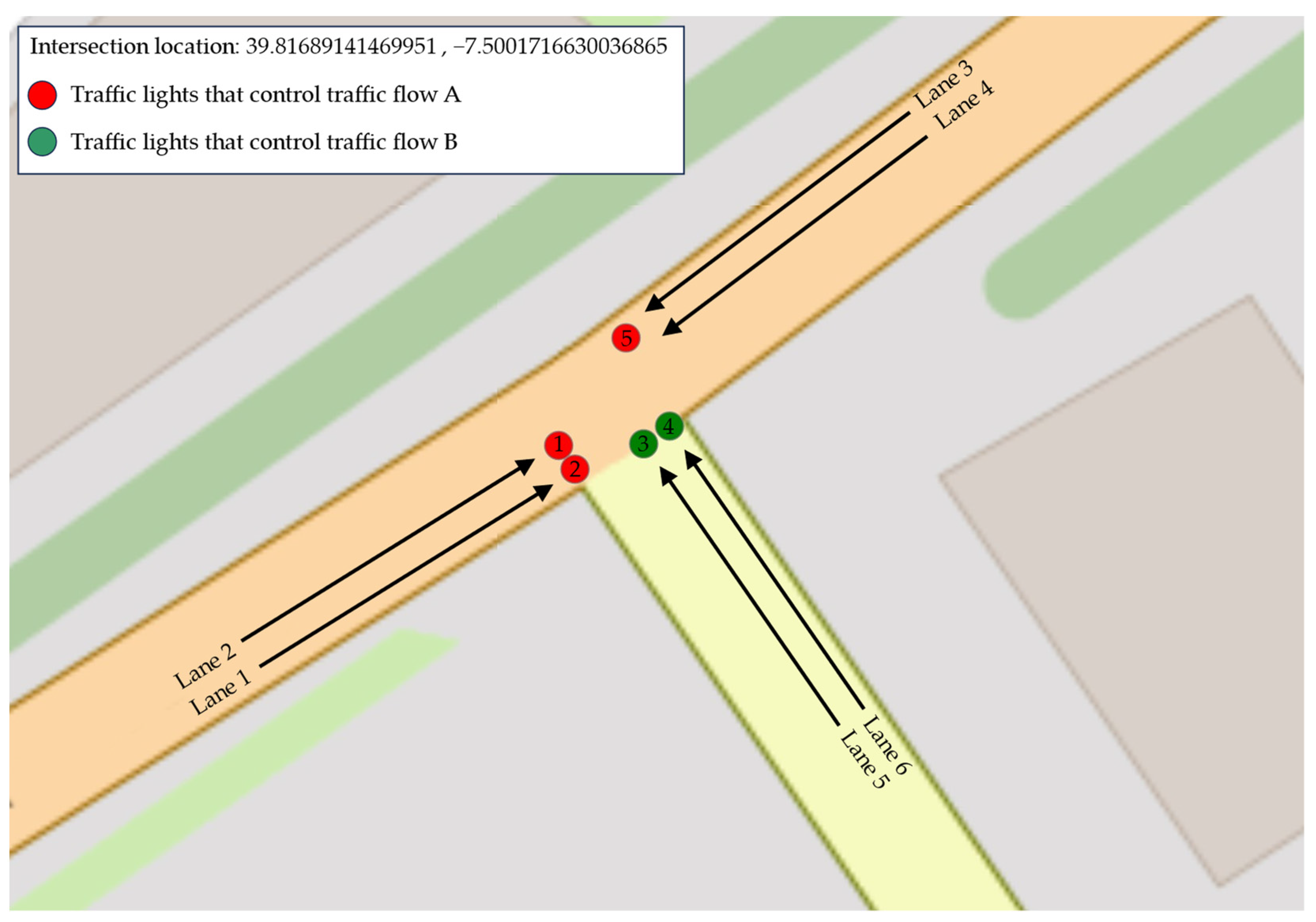
The simulation refers to a specific intersection in Castelo Branco, a small Portuguese city, with six inbound lanes, as can be seen in
Figure 1. This intersection has been chosen for the simulation because it is a key intersection that regulates traffic to/from the city centre.
The traffic profiles used in the simulation were created in the traffic profile creator tool, from base statistical parameters, gathered from the direct observation of traffic at the intersection. Four different traffic profiles were generated, with a time frame of one hour each:
A normal traffic profile corresponds to the regular traffic observed on weekdays, during the middle of the morning (10 a.m. to 12 a.m.) and afternoon (2 p.m. to 5 p.m.).
A high traffic profile corresponds to the traffic observed on weekdays, in the first hours of the morning (8 a.m. to 10 a.m.) and end of afternoon (5 p.m. to 7 p.m.).
A low traffic profile corresponds to the traffic observed in the early morning (from 6 a.m. to 8 a.m.) and night (from 8 p.m. to 11 p.m.).
A very low traffic profile corresponds to the traffic observed during the night, from 11 p.m. of one day to 6 a.m. of the next day.
To define the base statistical parameters for these profiles, each lane was observed for one hour during the profile time span, and the traffic was registered and classified. As an example,
Table 1 contains the statistical parameters observed at the intersection that were used to generate the normal traffic profile. There are no categories for battery electric vehicles (BEVs) or hybrid vehicles (HVs), because currently the percentage of BEV and HV vehicles in Portugal is so low that for the purpose of this study they can be ignored.
Then, each traffic profile was simulated by a passive routing strategy (fixed timing cycle), which mimics the existing traffic light system, and by a smart routing algorithm, especially designed to optimize CO2 emissions. The CO2 emissions, average speed, and waiting time for each simulation were registered and compared. The final step of the work was the assessment of the gains obtained with the smart routing algorithm, for different traffic densities, daily patterns, and a whole year of traffic.
Both the reliability and validity of the findings strongly depend on the overall reliability and accuracy of the simulator. For this reason, the simulator makes use of well-known and proven mathematical modelling (thoroughly described in
Section 4) of the energy that is required for specific vehicle kinematics and real-world data about the fuel that are needed to generate that amount of energy, considering the fuel type and vehicle class and mass. Moreover, the simulator has been tested with a single vehicle of each class, for different dynamic profiles, and the reported fuel consumption is consistent with expected reasonable values.
4. The Simulation Framework
This section describes the simulation framework, which has been developed specifically for this work. Although some well-established simulators such as VISSIM [
37] or SUMO [
38] could be used for the simulation, it was decided to build a new simulator from scratch. The main reason for this decision is that we wanted to have absolute control of every aspect of the simulation, including the different vehicles’ characteristics and kinematics, precise CO
2 emission estimation, and simulation of diverse driving styles. The goal was to create a simulator able to accurately reflect the reality of the traffic and driving styles at the target intersection.
The traffic simulation framework implements a microscopic model, a type of traffic model that describes traffic at the level of individual vehicles and their interaction with each other and the road infrastructure [
39]. The framework supports predefined traffic profiles, different types of vehicles, different driver behaviour models, and a set of rules that determine when vehicles accelerate, decelerate, brake, and change lanes.
The framework has been developed from the ground up to simulate a simple specific use case. However, a few design requirements were established to allow the framework to scale up to more complex scenarios and use cases if needed. These requirements include
The framework should be able to run on any typical general-purpose device.
The framework should be easy to deploy as a web-based application.
The framework should use open and free programming stacks.
The framework should include a visual interface, with the individual elements shown on a map.
These requirements led to the choice of popular and mature web technologies, such as HTML, JavaScript, Open Street Maps, and Leaflet. This technology stack allows the framework to run on any device with a modern browser and Internet connectivity.
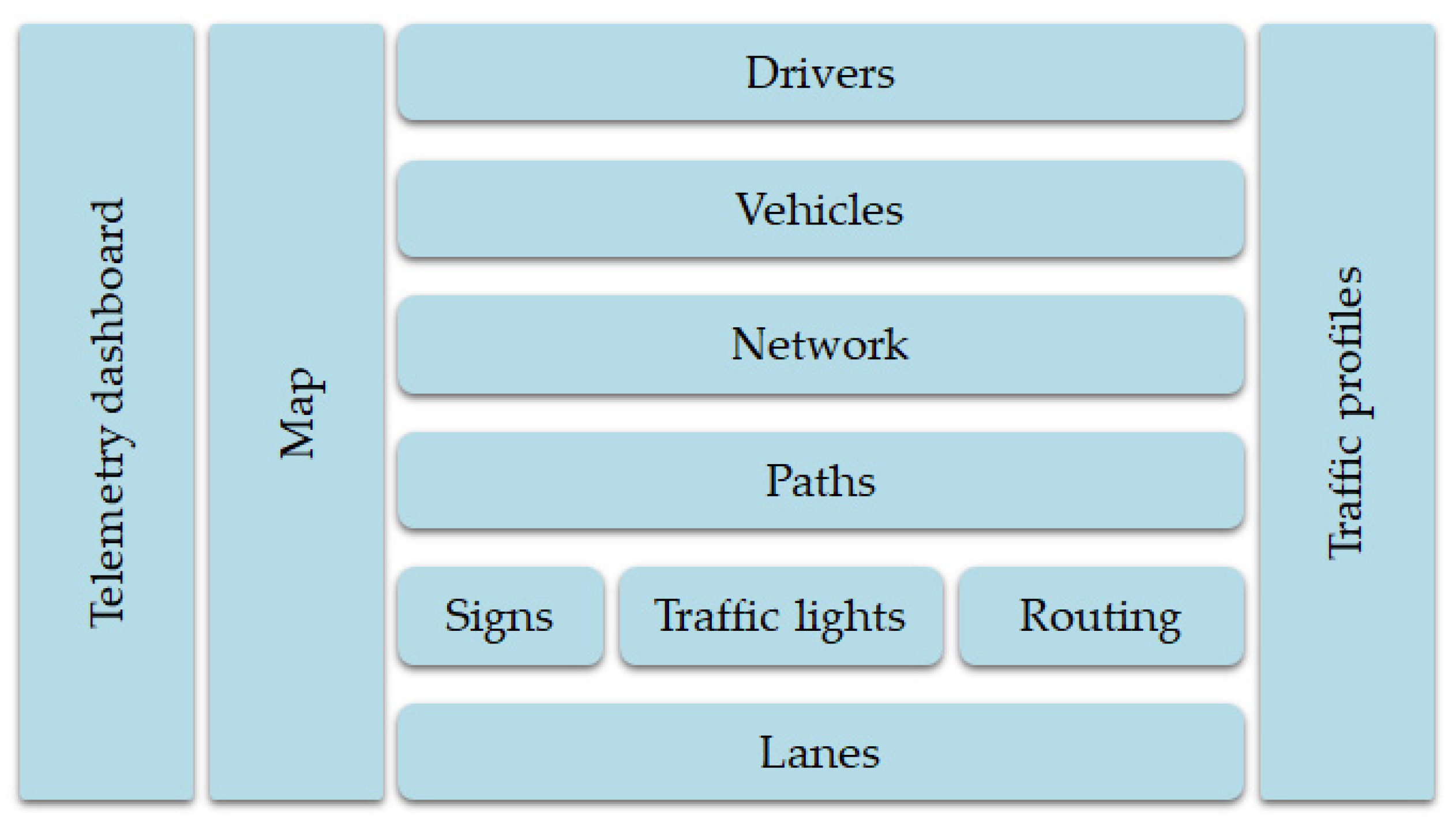
The framework has been designed as a layered architecture, using JavaScript object-oriented programming, with specific classes for each layer. This architecture can be seen in
Figure 2.
The main components of the framework are
Lanes: segments of road represented by polylines, for a single line of vehicles.
Traffic lights: an element that controls the flow of traffic from one lane to another.
Routing: how traffic lights are controlled.
Paths: how lanes are interconnected.
Network: the set of paths that can be travelled by vehicles.
Vehicles: individual vehicles, each one with its own characteristics, that can travel across the network.
Drivers: a model that tries to mimic individual and diverse driving styles.
Map: a graphical representation of the network, traffic lights, and vehicles.
Telemetry dashboard: a dashboard to visualize the statistics of the simulation.
Traffic profiles: pre-recorded traffic profiles that can be injected into the simulator, to test the results of different routing strategies.
4.1. Lanes, Paths, and Traffic Lights
A lane is a segment of road represented by a polyline of GPS points, where a single line of vehicles may travel in an ordered way. A lane allows only one traffic flow in a single direction; to simulate roads that allow multiple parallel traffic flows, a different lane is required for each traffic flow.
Lanes are implemented as objects of a JavaScript class. The lane path is represented as an array of GPS points that form a polyline, where the vehicles travel. The polyline resolution is variable and defined by code; in this case, the minimum distance between adjacent points is 10 cm, to allow for smooth curvatures. Lanes also have information about their slope (road inclination), which is a very important factor to determine fuel consumption and therefore CO2 emissions.
Lanes have a fixed speed limit and slope for all their points; to simulate a road segment with different speed limits or slopes, several lanes must be interconnected one after the other. Each lane keeps a record of the vehicles travelling inside that lane, and their position as well. The lane class has methods to determine what is ahead of each vehicle, and its distance and speed, if applicable. These methods are crucial to govern the movement of each vehicle in the lane.
The lane class also has methods to obtain telemetry data, which include the number of vehicles in the lane, the number of vehicles waiting for the traffic flow to resume (for example, when a traffic light is red), and the cost of stopping the traffic flow in the lane—this will be explained later in another section.
A path is a sequence of interconnected lanes that can be travelled by a vehicle. There are several different ways to interconnect lanes into a path:
Direct connection between two lanes: In this case, the end of one lane connects to the start of the other lane, without any traffic control in the transition. Vehicles move from one lane to the other lane without hindrance, except for a possible different speed limit in the next lane.
Connection through a traffic light system: In this case, the end of a lane connects to the next lane through a traffic light system. Vehicles must observe the colour of the traffic light before entering the next lane.
Connection through a stop or priority sign: In this case, vehicles enter the next lane, not at its beginning but at a specific position in the lane. Before entering the lane, vehicles must comply with the control sign, either a stop sign or a priority sign—either explicit or implicit—such as when entering a roundabout.
Paths can also create branches: at the end of one lane, traffic can be routed to several different lanes, according to a parameterised probability distribution. Different lanes can merge into a single lane as well. The network layer comprises all the paths in the simulation, from where the statistical information is gathered.
Traffic lights are implemented as a class, which thereby determines how the vehicles behave when approaching an intersection controlled by traffic lights. Traffic lights have a visual representation on the map as well: red, yellow, or green circles, which help to visualize how vehicles behave at traffic lights.
This class has two versions: one that implements the fixed time cycle system that is currently deployed at the intersection and another version, which implements the smart routing algorithm.
4.2. Vehicles and CO2 Emissions’ Estimation
The vehicle JavaScript classes model the behaviour of vehicles, from kinematics to CO2 emissions, and are the most important classes in the simulator. The class structure is based on a superclass called classVehicle that models the characteristics that are common to all the vehicles. This superclass has a set of properties that are defined in the class constructor, which include
carLength: car length in meters; this is used for modelling the space that the vehicle takes in the lane.
carWeight: car weight in kg, which is used to calculate the energy needed to accelerate the vehicle and therefore the fuel consumption and CO2 emissions.
initialCarSpeed: initial car speed in m/s (the speed of the vehicle when it is inserted into a lane).
hasStartStop: a true/false flag that indicates whether the vehicle is equipped with a start–stop system.
carAcceleration: the maximum acceleration capability of the vehicle in m/s2.
noGasAcceleration: the vehicle deceleration in m/s2 (negative value) if no pressure is applied on the acceleration pedal.
lowBrakingAcceleration: car deceleration in m/s2 (negative value) in a soft braking.
mediumBrakingAcceleration: car deceleration in m/s2 (negative value) in a normal braking.
hardBrakingAcceleration: car deceleration in m/s2 (negative value) in a strong braking.
fullBrakingAcceleration: car deceleration in m/s2 (negative value) in an emergency braking.
Besides these common characteristics, seven subclasses were created to model different types of vehicles and fuel: smallPetrolCarClass, smallDieselCarClass, bigPetrolCarClass, bigDieselCarClass, mediumVanClass, bigVanClass, and busClass. As a result of a direct observation of the intersection, these different vehicle types are the most prevalent in normal city traffic. A different icon is associated with each vehicle type, to create a visual distinction on the map.
Each one of these classes has a different method to calculate the fuel consumption and CO2 emissions, because these calculations depend on the type of fuel and type of vehicle. The next section describes how CO2 emissions are calculated.
One crucial feature of the simulator is the estimation of fuel consumption and emitted CO
2 by each vehicle, in its different operation modes, e.g., accelerating, decelerating, braking, idling, or cruising. This estimation is based on the concept of vehicle specific power (VSP) [
40], which can be described as the instantaneous tractive power per unit vehicle mass.
The VSP parameter reflects most of the dependence of vehicle emissions on driving conditions; thus, it has been extensively used to estimate second-by-second emissions and fuel consumption, given the roadway grade (slope), vehicle speed, acceleration, or deceleration [
41]. One major advantage of using the VSP as the fundamental parameter for emission models is that it is calculated independently from the type of vehicle, type of fuel, or even the vehicle weight. Therefore, VSP allows significant comparisons to be made between data from different dynamometer driving cycles, vehicles, and emission models; hence, it is widely used in vehicle emission models, such as EPA’s MOVES model [
42].
The VSP is expressed as W/kg (or kW/metric ton) and calculated with Equation (1).
: vehicle-specific power in W/kg
: vehicle velocity in m/s
: vehicle acceleration in m/s2
: road slope in percentage
This formula is based on [
40] (p. 55), excluding the headwind effect, which is not considered in the simulator, because the wind factor is not relevant to the goal of this study. The VSP is a general parameter for every vehicle; therefore, it is calculated in the Vehicle JavaScript super class. The VSP parameter is dynamic over the course of time and must be calculated as vehicles change acceleration and speed. The frequency of VSP calculation is parameterizable in the framework; in this use case, it is calculated with a frequency of 10 Hz, i.e., using 100 ms time slots.
Fuel consumption and CO
2 emissions are then calculated for each time slot, using the methodology of CONOX project task 1 [
43] (p. 15), which describes a model to calculate emissions from the VSP parameter and vehicle characteristics, based on real-world driving measurements. According to this model, the instantaneous fuel consumption (in grams per hour) can be estimated with Equation (2).
: fuel consumption in g/h
: factors that depend on vehicle type
: vehicle mass in kg
Factors A, B, and C depend on the type of car and fuel. This framework uses the generic data to be used per vehicle segment or for average diesel and gasoline vehicles, as suggested by the CONOX report [
43] (p. 15).
Table 2 shows the values for the three factors, for each vehicle type of the framework.
Finally, having computed the fuel consumption, the last step is to calculate the CO
2 emissions for each time slot. This is performed by converting the consumed fuel mass to CO
2 emissions—assuming that most of the carbon in the fuel is converted to CO
2. The conversion factors are based on [
44] (p. 7) and are, respectively, 3.163 kg of CO
2 per kg of diesel and 3.171 kg of CO
2 per kg of petrol.
4.3. Driver Behaviour and Traffic Profiles
Since its inception, one major design requirement for the simulator was that it should model realistic vehicle kinematics, especially in the way of how real drivers behave. To accomplish this, four different driving style dimensions were identified, which model the main aspects of driver behaviour. These dimensions are described as the following properties:
securityDistanceToObjectAhead: typical security distance that the driver keeps to the object ahead (other vehicle, traffic light) in meters.
reactionTime: Typical reaction time of the driver, in seconds; an example is when a traffic light turns green or when a stopped car ahead starts moving. This property is crucial to mimic the inertial effect observed in a lane of stopped vehicles, when the first vehicle starts moving.
driverAggressivity: A value from 0 to 1, which models the way of how the driver uses the performance capabilities of the car (acceleration and braking). A value of 1.0 means that the driver uses the full acceleration and braking power of the vehicle.
speedLimitComplianceFactor: A value around 1 that represents how the driver respects the speed limits. A value of 1.0 means that the driver scrupulously respects the speed limit; 1.1 means that they exceed the limit by 10%; 0.9 means that they drive 10% below the speed limit.
In a simulation, each vehicle can be associated with a different, unique driver profile. This profile can be created randomly within a normal distribution around a typical value, which results from the direct observation of typical driver behaviour at the intersection.
This randomness, combined with the diversification of the vehicle’s characteristics, means that the probability of having two vehicles exhibiting the same behaviour is kept very low. This uniqueness not only tries to replicate the randomness that is observed in real traffic, but also ensures that there are no unexpected simulation effects of having several vehicles exhibiting the same behaviour.
To test and compare different routing strategies in the same conditions, the framework allows creating and testing traffic profiles. A traffic profile is a file associated with a lane, which defines when a vehicle enters that lane, its type and characteristics, and the driver profile as well.
The traffic profile files are generated using a specific tool of the framework, which creates a profile file from a set of statistical characteristics obtained from the real traffic patterns observed at the intersection. The tool generates a random distribution of vehicles of different types, different characteristics, and a random driver profile for each vehicle. This randomness ensures that each vehicle has a unique, individual behaviour, thus avoiding the eventual unexpected effects of having a set of vehicles with the same behaviour in the lane. Moreover, the direct observation of the intersection revealed this kind of randomness in the real traffic.
The tool that generates the traffic profiles requires the following parameters: estimated number of vehicles per hour, total time of the profile, average entry speed into the lane, and burstiness, which determines how the vehicles are distributed along time. Higher values of burstiness mean that the vehicles have a high probability to pack in groups of several vehicles. The tool also requires the probability for each type of vehicle, thus enabling the creation of profiles with a very different distribution of vehicle types.
4.4. Data Collection
Data collection is made at the vehicle level: each vehicle object registers its fuel consumption, CO
2 emissions, velocity, waiting time (when it stops at a traffic queue), and travelled distance. Data are then gathered at lane, path, and network levels. The consolidated data are then shown to the user on a simple dashboard, which exhibits the total number of vehicles in the simulation, the total travelled distance, the average speed, the total waiting time, the average CO
2 emissions by vehicle, and the total CO
2 emissions of the simulation.
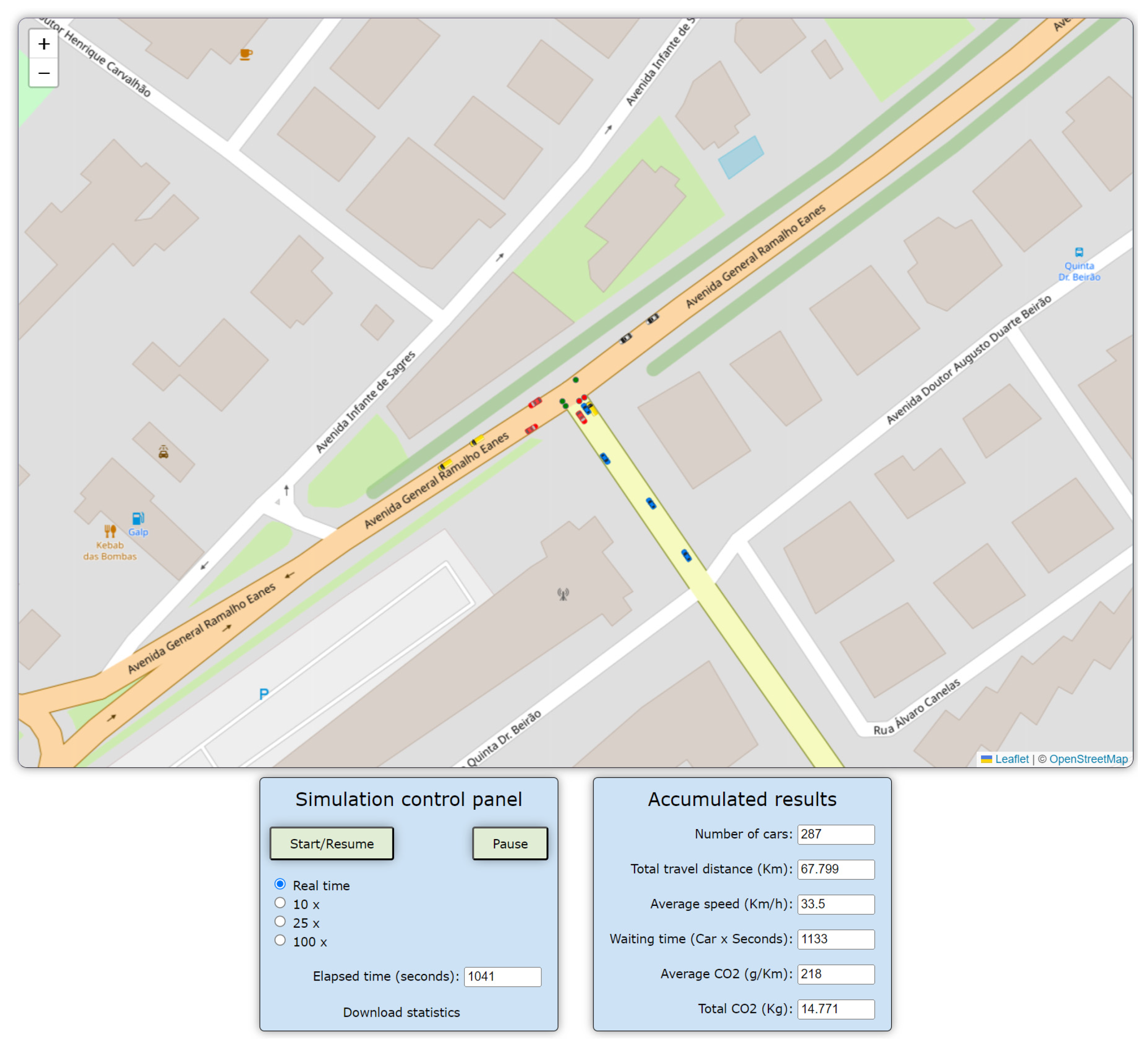
Figure 3 shows the overall graphical interface of the simulator.
Videos are also available online [
45,
46] that show the simulator in operation.
5. Simulation Results
The current traffic light system is a basic passive system, which runs a fixed sequence of states, with a predetermined allowance time for each traffic flow. This sequence, which is shown in
Table 3, has been directly observed at the intersection and then coded into the traffic light class. After state 5, the system restarts at state 0.
As can be seen in
Table 3, states 0 and 3 are the most important states (those that allow traffic to flow between lanes). The other states prepare the traffic flow transition (states 1 and 4) and block all the traffic for some seconds to avoid collisions (states 2 and 5).
The simulation was run ten times, and the average values were gathered, because the simulation results are not always the same, even with the same traffic profiles. This happens because there is a path in the network where vehicles can choose one of two different lanes, and this choice is random and made at run-time. Therefore, each simulation is slightly different, and the results are marginally different as well.
Table 4 shows the results for the normal traffic profile, with the current traffic light system:
These average values are the base reference for the results obtained with the smart algorithm. The average CO2 emission per vehicle (318.6 g/km) is higher than anticipated, but it can be explained by the high number of vehicles that need to accelerate from a stop, a condition that is not favourable for fuel economy and CO2 emissions.
5.1. The Base Active Algorithm
Even using the most efficient and optimized algorithms for vehicle routing, internal combustion engine (ICE) vehicles will always have to burn fuel and emit CO2 when crossing the intersection. Therefore, it is useful to estimate what would be the best possible achievable reduction in CO2 for this scenario, to have a reference that active algorithms can be compared with.
The best possible results would be achieved if all the vehicles could traverse the intersection without being blocked by a red traffic light. Of course, this scenario is not feasible in the real world, but it can be simulated, by running the two concurrent traffic flows one at a time and keeping the respective traffic lights always green. This was performed, and the combined results for the CO2 emissions were 193 g/km, which means that the maximum reduction in emissions that an optimized algorithm can obtain is about 39%. However, this limit would only be achievable if the traffic flows were perfectly nonconcurrent and synchronized, something which is highly improbable in the real world.
One design requirement for the active routing algorithm is that it can only use information able to be gathered by a real system, using cameras or other sensors, so that it can be deployed in the real world if needed. Therefore, the algorithm only has access to the number of cars that are approaching the intersection, their position, and their speed; all these data can be obtained by cameras. The algorithm has no access to the category of a vehicle, its fuel type, or other vehicle-specific characteristics. The vehicle visibility is also confined to the 150 m of each lane near the intersection.
The base active algorithm follows a typical approach that decides based on the estimated costs of all the options. In this use case, there are two major traffic flows, and the algorithm is continuously computing the cost of stopping each traffic flow. When the cost of keeping the stopped traffic flow blocked is higher than the cost of stopping the active traffic flow, a switch in the traffic lights is initiated. The cost of each traffic flow is calculated with Equation (3).
: vehicle speed in m/s
: constants
The J and K constants are used to model the weight given to the simple presence of a vehicle (constant J) and to its kinetic energy (constant K) to the overall cost. As a matter of fact, from the CO2 emission perspective, the cost of blocking a lane with moving vehicles is expected to be higher than blocking a lane with stopped or slow vehicles, because stopping moving vehicles wastes kinetic energy that needs to be restored later by burning fuel when the vehicles re-accelerate.
The algorithm has safeguards to prevent a traffic flow being blocked or allowed for an unreasonable amount of time. Hence, both traffic flows are enforced with a minimum allowed time of 10 s and a maximum allowed time of 180 s, values that were considered reasonable. These limits have priority over the decision based on costs.
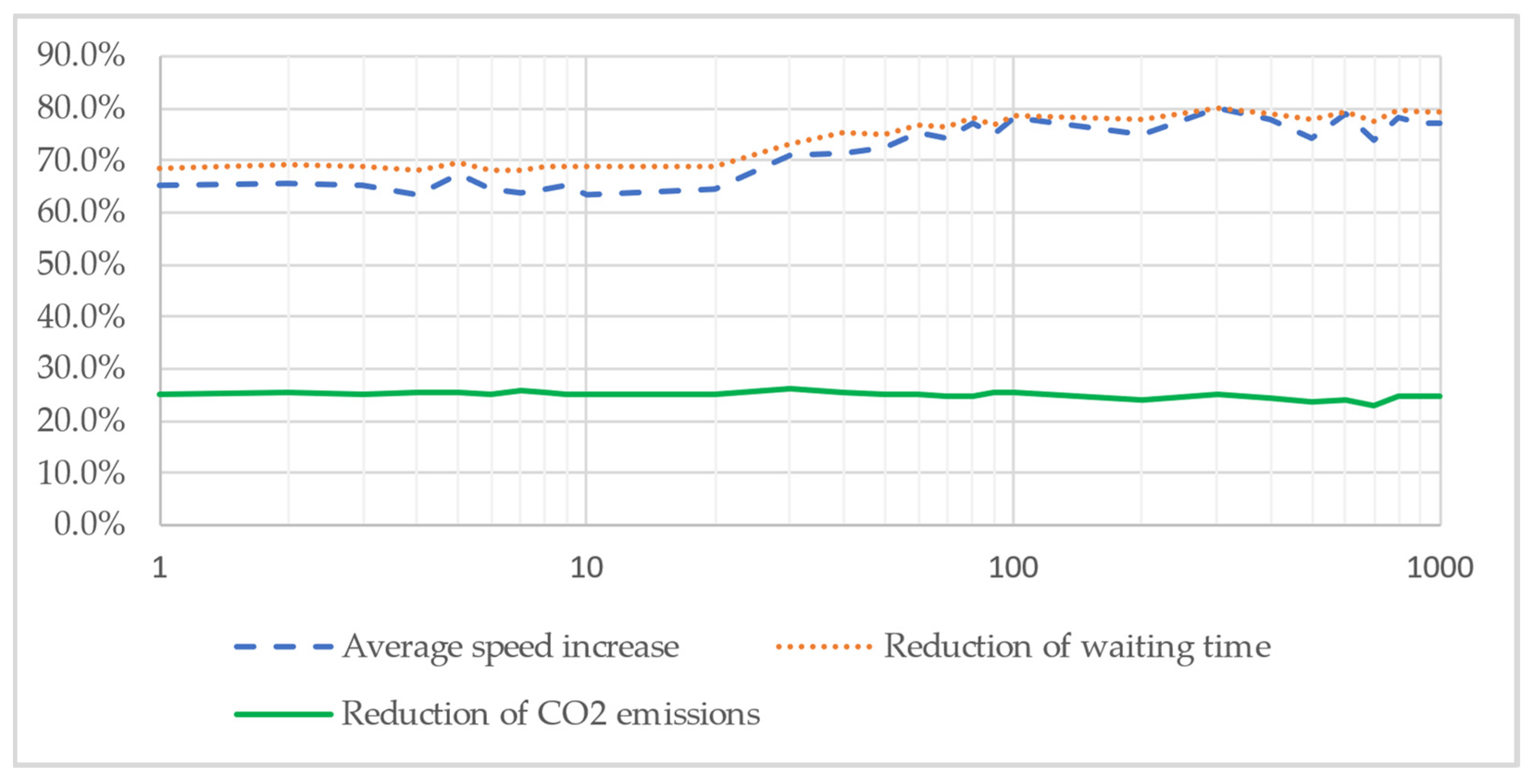
This algorithm was tested, keeping the constant K = 1 and varying J from 1 to 1000, in logarithmic steps. A low value of J means that the cost depends almost exclusively on the vehicles’ speed whereas a high value of J means that the cost depends mostly on the number of vehicles in the traffic flow, regardless of their speed. The results of this testing stage can be observed in
Figure 4.
The outcomes from the simulation include results that were expected, such as a substantial reduction in CO2 emissions (between 23% and 26%), but also some unexpected results, such as the extraordinary improvements (up to 80%) in waiting time and average speed. Another unexpected aspect of the simulation is that the effect of constant J in the CO2 emissions is almost insignificant; as a matter of fact, the CO2 emissions’ reduction does decline as J increases, but the difference is very small. This means that the results depend mostly on the number of cars in a traffic flow, rather than their speed.
However, the constant J does have a relevant effect on average speed and waiting time. As can be seen in
Figure 4, between J = 20 and J = 100, there is a steady improvement in both indicators, about 10% in waiting time and 15% in average speed. Values of J higher than 100 do not improve waiting time or average speed, but have a small negative impact on CO
2 emissions; thus, the optimal value for J is around 100.
5.2. Enhancing the Algorithm
As described in the previous section, the weight of vehicles’ speed in the cost formula had a small impact in the overall CO2 emission results. This is somehow counter-intuitive, so this issue was further investigated. The real-time observation of the results of the cost formula with the traffic flow and vehicle behaviour gave an insight into the reasons for this unexpected result. As a matter of fact, the problem is that both traffic flows use the same cost formula, but a moving vehicle in a blocked lane should not have the same cost as a moving vehicle in an allowed lane, as the former will almost certainly have to stop, because switching the traffic lights takes some time.
Therefore, the cost formula was changed to increase the weight of vehicles’ speed, but only in the traffic flow that is allowed at that time. This was carried out by changing the K constant from 1 to 30; this value was considered as the optimal one, after experimenting with several values. After this tweak, the results for CO
2 emissions improved by 2.8% more, the awaiting time by 1.3% more, and average speed by 5.8% more. These results are shown in
Table 5.
Another potential improvement that was investigated is related to the safeguard periods, the small periods of time with both traffic flows blocked (all the lights red), designed to prevent collisions should a vehicle not comply with the yellow light. In passive systems, this safeguard is crucial to avoid accidents, but active systems can be aware of the vehicles’ behaviour at the intersection; thus, this safeguard can be safely bypassed if the traffic flow, which is being blocked, is already stopped at the yellow light or if there are no vehicles near the intersection in the lanes being blocked.
Thus, the algorithm has been tweaked to bypass the safeguard periods when it is safe do it, and the results are substantial: CO
2 emissions improved by 3.8% more, the waiting time by 3.4%, and the average speed by 10.4%.
Table 5 shows the overall results for each stage of the algorithm.
The CO2 emissions’ improvement is significant, if we consider that the maximum improvement possible for this traffic profile is 39%, and only if the traffic flows were nonconcurrent, something that is highly unrealistic.
5.3. Results with Other Traffic Profiles
In the previous section, results were obtained from several rounds of testing, always with the normal traffic profile, which inserts 566 vehicles per hour in the intersection. However, traffic patterns vary throughout the day; thus, it is important to test the algorithm with traffic profiles with lower and higher vehicles’ densities.
Three other traffic profiles were generated from direct observation of the intersection in key moments: a very low traffic profile (56 vehicles per hour), a low traffic profile (566 vehicles per hour), and a high traffic profile (1679 vehicles per hour).
Table 6 shows the results of the simulation with these different traffic profiles. It also contains the results with the normal traffic profile, which had been previously obtained. The passive routing and the smart routing are identified in the titles by the P and S prefixes, respectively.
Observing the results, some aspects stand out:
As expected, as the traffic density increases, all the indicators get worse, both in passive and smart routing.
The smart algorithm achieves substantial gains in speed, waiting time, and CO2 emissions in all the traffic profiles.
The lower the traffic density, the higher the gains.
5.4. Simulating a Whole Day of Traffic
The final tests simulated a whole day of traffic, from 0H00 to 23H59, with variable traffic density throughout the day. Two different daily profiles were tested: a weekend profile, which has normal traffic during the day, and a weekday profile, which has three periods of high-density traffic (early morning, midday, and late afternoon). The simulation results can be seen in
Table 7. The passive routing and the smart routing are identified in the titles by the P and S prefixes, respectively.
The gains achieved by the smart routing algorithm for the weekday are not as good as those of the normal traffic profile; this can be explained by the influence of the three periods of high traffic density. Not surprisingly, results for the weekend profile are better, almost reaching those of the low traffic profile. As a matter of fact, the CO2 reduction (−40%) equals the same result of the “very low” profile.
These simulations for a whole day give an insight on the total daily reduction in CO2 emissions that can be achieved by a smart routing algorithm. In this case, the potential reduction is 381 kg for a weekday and 362 kg for a weekend day.
5.5. Effects on Other Road Users
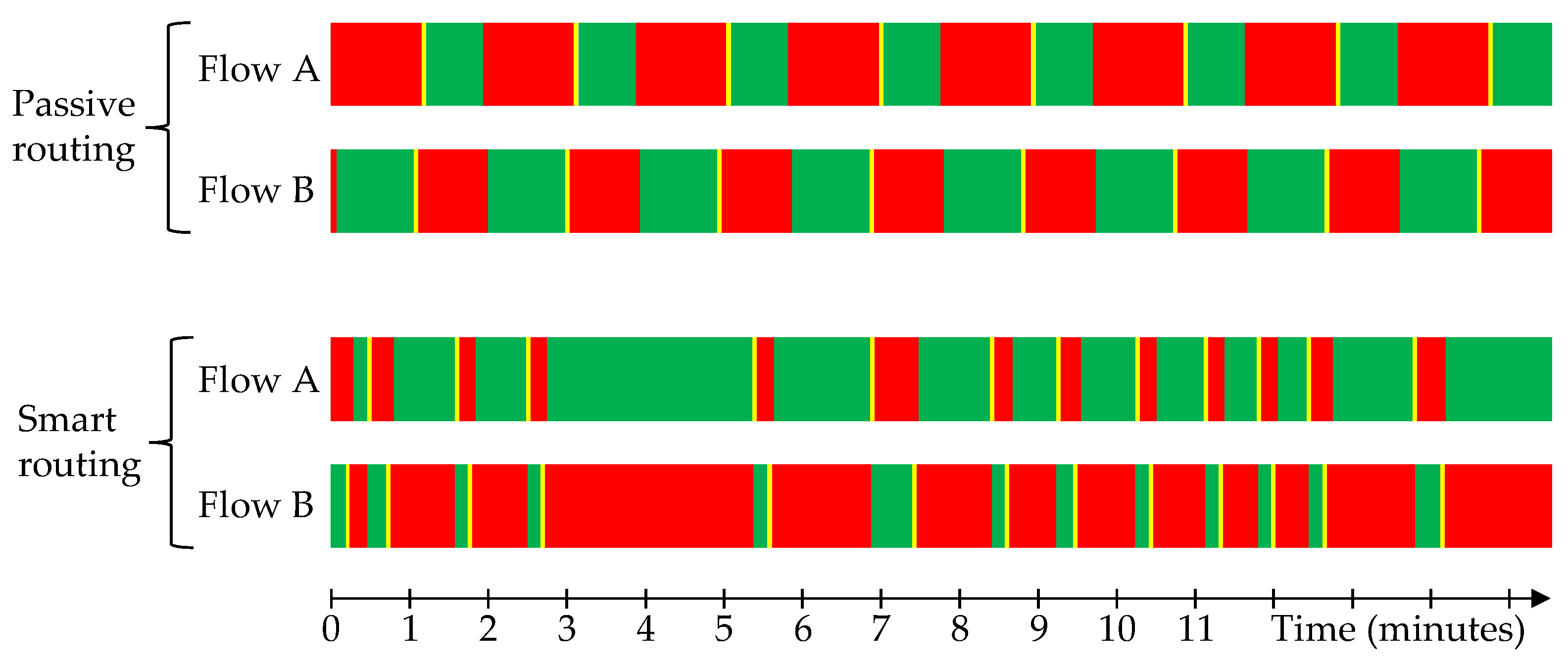
Changing the traffic light timings from a fixed cycle to a dynamic cycle means that the duration of the red and green phases is no longer predictable or balanced, as it is actively determined by the traffic dynamics.
Figure 5 shows a snapshot of 15 min of traffic routing with both strategies, which illustrates how the cycle timings generated by the smart routing algorithm can be irregular and unbalanced.
This variability and unpredictability could affect other users who share the same infrastructure, such as pedestrians. There are two crosswalks at the intersection, concurrent with each traffic flow, and pedestrians can only use them when the traffic flow is stopped, so they are affected by the frequency and duration of the red phase of the respective traffic flow.
To investigate the effects of the smart routing algorithm on pedestrians, the cycle times were recorded using the normal traffic profile, and two indicators were calculated: the average waiting time until pedestrians can use the crosswalk (assuming that pedestrians arrive at the crosswalk at arbitrary times) and the average time window to cross it. The results are shown in
Table 8; the passive routing and the smart routing are identified in the titles by the P and S prefixes, respectively.
As can be observed in
Table 8, both the indicators for crosswalk B were improved by the smart routing algorithm, with a substantial reduction in waiting time. However, at crosswalk A, both indicators have worsened: the waiting time is just slightly longer, but the average crossing window has been significantly reduced. This can be a problem at intersections with a high number of pedestrians (which is not the case here), but the algorithm can be parameterized to impose larger time windows for pedestrians. However, limiting the algorithm’s freedom will have an impact on its performance regarding optimization of CO
2 emissions.
Other road users who could be affected by the intelligent algorithm are cyclists. There are no dedicated lanes for cyclists at this location, so modelling their behaviour is challenging, as they usually move erratically in traffic, especially when the flow of traffic is at a standstill. However, the results from the simulations show that the average waiting time for any vehicle is substantially reduced, regardless of the type of vehicle or lane. This means that an arbitrary vehicle (including users that do not produce CO2 such as cyclists) has a high probability of benefiting from the smart traffic routing algorithm. This is explained by the fact that this optimization problem is not a “zero sum game”; the gains are obtained mostly by eliminating the inefficiencies of the traditional fixed cycle traffic lights and not by delaying other vehicles.
6. Conclusions
The microscopic traffic simulation framework proposed in this work can be very useful to simulate realistic vehicle kinematics and driver behaviour, and to estimate CO2 emissions accurately.
The simulation with different traffic profiles shows that deploying smart traffic lights at a single intersection can reduce CO2 emissions by 32% to 40% in the vicinity of the intersection, depending on the traffic density. These figures are very close to the maximum possible gains; for example, the 32% reduction with the normal traffic profile is very close to the maximum possible reduction, which is 39% in optimal conditions, i.e., nonconcurrent traffic flows. However, nonconcurrent traffic flows are implausible in the real world.
In addition to reducing CO
2 emissions, drivers can also benefit directly from smart traffic routing. Indeed, as CO
2 emissions are directly proportional to the quantity of fuel that is burned, a reduction in fuel consumption between 32% and 40% is also expected. The simulation also highlights other advantages for drivers: an increase in the average speed between 60% and 101% and a reduction in waiting time from 53% to 95%, depending on the traffic density. These relative gains are substantial, but the absolute values are even more impressive: for example, in the normal traffic profile, the average waiting time drops from 25 s to just 4 s. These results are better than those obtained in the studies described in the
Section 2; however, the type of intersection and traffic profiles are different from study to study; hence, comparing these results is questionable.
The annual absolute figures, obtained by extrapolating the daily results to a full year, are noteworthy: less 136 tons of CO2 emissions, less 32,000 h of waiting time, and less 55,000 litres of fuel consumed, which at current local prices cost about EUR 98,000. Therefore, regarding the main research question of this work, the conclusion is that it is worth deploying smart traffic lights in small cities to reduce CO2 emissions and improve traffic flow.
The use of the simulator in this case study shows that it can be a useful tool for simulating realistic vehicle kinematics and driver behaviour and, consequently, to help define smart routing algorithms for traffic lights. This will directly contribute to improving traffic flow and to optimize CO2 emissions at intersections. This type of tools and results can help city-level decision makers with mobility policies in small cities or environmental impact researchers to make optimized and efficient decisions, not only in terms of managing traffic flows but also to reduce their environmental impact.
Future Work
This work focused on the simulation of a single intersection of a small city. The results for a single intersection are already conclusive, but even better results are expected when several linked intersections are simulated together, and the smart routing algorithm uses scattered data and coordinates all the traffic lights at those intersections. Therefore, one path for further research would be to simulate a wider area of the city, or even the whole city.
Another approach that is worth exploring is using artificial intelligence methodologies to control smart traffic lights. The tools that were developed in this work can be easily tweaked to generate and simulate thousands of random traffic patterns to make a large dataset that can be used to train a machine learning model. The next step is to investigate whether an artificial intelligence model can outperform the smart algorithm developed in this work.


