Study of a Square Single-Phase Natural Circulation Loop Using the Lattice Boltzmann Method


DIME—Department of Mechanical Engineering, Energy, Management, and Transportation, Division of Thermal Engineering and Environmental Conditioning, University of Genoa, Via All’Opera Pia 15-A, 16145 Genova, Italy
*
Author to whom correspondence should be addressed.
Appl. Mech. 2023, 4(3), 927-947; https://doi.org/10.3390/applmech4030048
Submission received: 26 May 2023
/
Revised: 24 July 2023
/
Accepted: 10 August 2023
/
Published: 28 August 2023
(This article belongs to the Special Issue Applied Thermodynamics: Modern Developments (2nd Volume))
Abstract
:Natural circulation loops are thermohydraulic circuits used to transport heat from a source to a sink in the absence of a pump, using the forces induced by the thermal expansion of a working fluid to circulate it. Natural circulation loops have a wide range of engineering applications such as in nuclear power plants, solar systems, and geothermic and electronic cooling. The Lattice Boltzmann Method was applied to the simulation of this thermohydraulic system. This numerical method has several interesting features for engineering applications, such as parallelization capabilities or direct temporal convergence. A 2D model of a single-phase natural circulation mini-loop with a small inner diameter was implemented and tested under different operation conditions following a double distribution function approach (coupling a lattice for the fluid and a secondary lattice for the thermal field). An analytical relationship between the Reynolds number and the modified Grashof number was used to validate the numerical model. Two regimes were found for the circulation, a laminar regime for low Reynolds numbers and a non-laminar regime characterized by a traveling vortex near the heater and cooler’s walls. Both regimes did not present flux inversion and are considered stable. The recirculation of the fluid can explain some of the heat transfer characteristics in each regime. Changing the Prandtl number to a higher value affects the transient response, increasing the temperature and velocity oscillations before reaching the steady state.
1. Introduction
Natural circulation loops (NCLs) are engineering systems used to transport heat from a source to a sink by the motion of a working fluid induced by the thermal expansion. It is interesting because this kind of thermal circuit can work without a pump or a recirculation system [1]. NCLs find application in several fields such as electronic cooling, geothermic cooling, solar systems, and nuclear power plants [2]. The working fluid can be in a single phase (e.g., water in the liquid phase or air in the gas phase) or have two phases. In the rest of this work, the focus will be on a single-phase NCL.
Some analytical relationships can predict the flow characteristics of the loops under selected operational parameters such as geometric dimension, fluid properties, source, and sink characteristics for laminar regimes [3] and transition or turbulent regimes [4]. These relationships have been validated by comparison with experimental data from laboratories around the world. The stability of an NCL is a primordial problem because, under some operational parameters and loop geometries, the flow direction can be inverted, and the system flow can become chaotic [5], an undesirable situation for critical engineering applications that require predictable heat flux removal. In recent years, experimental works have found that localized pressure losses can stabilize the loops [6], and it was also found that an NCL with a small inner diameter is stable and can work connected in parallel [7,8] with small disturbances even if the power provided to one parallel loop changes.
Previous works have evaluated the performance of rectangular-shaped, single-phase NCLs with end heat exchangers mainly by developing analytical models, simulations, or experiments. One early computational work used a one-dimensional model (Rao, 2002 [9]). This model considers the temperature profiles along the end heat exchangers, which work in counterflow (heater and heat sink). Later, finite element method simulations were developed by Rao et al., 2005 [10]. They developed a one-dimensional model (including equations for the end heat exchangers) to test the effect of different thermal excitation functions on the time to reach the steady state. They found that the maximum and minimum temperature values during the transient response are equal, but there was a delay in the circuit response, this delay changes for each excitation simulated (ramp, step, and exponential). This one-dimensional approach allows for the calculation of a longitudinal temperature profile along the NCL pipes. Additional studies focused on dynamic and total pressure variation (Rao et al., 2008) [11]. A single-phase CO2 NCL with end heat exchangers has been investigated in a steady state using finite differences and the one-dimensional model developed by Kumar and Gopal in 2009 [12], who validated their approach by comparing the results with analytic expressions for the temperature and volume flow rate.
Yadav et al., 2012 [13], simulated a rectangular NCL with end heat exchangers using a CFD model. They propose a nondimensional correlation for the Reynolds number and the modified Grashof number in the turbulent regime (7000 < Re < 360,000). Later, Yadav et al., in 2014 [14], performed a simulation with different tilt angles and found that the tilt angle increases the mass flow rate and decreases the heat exchange. Moreover, they also found that a higher operating pressure reduces the time to reach the steady state. They corroborated the Swapnalee and Vijayan empirical correlation for the turbulent regime [3] as well as the previously proposed computational correlation [15] (valid from 27,000 < Re < 180,000). Both correlations have small changes but take the same functional form. Cheng et al., in 2018 [16], using a 3D CFD model, simulated the transient response of a single-phase NCL, evaluating the mass flow rate and energy generation. They used Vijayan’s correlation [3,17] for the laminar regime (originally proposed for imposed heat flux at the heater) with a good fit for the tested Reynolds numbers (lower than 100). The simulation showed a temperature gradient on the heat exchanger walls, generating an asymmetric condition. Recently, a study on the jump in the heat transfer coefficient by tilting the square NCL (single and coupled) was conducted using 2D and 3D numerical models, with a simplified geometrical model (Dass and Gedupudi, 2021) [18].
In the above papers, the numerical simulation employed the classic techniques of CFD. In this paper, to study a single-phase NCL, the Lattice Boltzmann Method (LBM) was adopted.
The LBM is a numerical method characterized by a mesoscopic approach [19,20], a middle point between the macroscopical approach of Navier–Stokes-based models (e.g., finite element methods) and a microscopic approach (e.g., molecular dynamics methods). The LBM considers the evolution of the probability density function by discretizing the Boltzmann equation. Macroscopic variables (local density, momentum, and temperature) are calculated by integrating the density function over the discretized velocity space. This method is highly parallelizable via its local algorithmic rules. It can handle multi-physics simulations by considering different lattices simultaneously, i.e., one lattice for the fluid density and momentum and a second lattice for the temperature field, and some other lattices if phenomena such as neutral particle transport or chemical species transport are of interest [21]. The simplest LBM, called Bhatnagar–Gross–Krook (BGK), is characterized by a single-relaxation-time collision operator [22] and can reproduce the Navier–Stokes equation for semi-incompressible flows at low Mach numbers, but the model is limited to isothermal flows.
Different upgrades of the LBM have been developed to account for thermal effects, as was presented in the recent review by Sharma et al., 2020 [23]. Various approaches exist for simulating heat transfer with LBM, including multispeed models, double distribution function (DDF) models, and hybrid models that combine LBM for solving the Navier–Stokes equation and another method (like finite differences) for solving the energy equation. Multispeed models involve an expanded velocity base, allowing for the direct calculation of internal energy as the third-order moment of the density distribution function. On the other hand, the DDF approach employs two lattices to describe the density and the thermal field. Internal energy conservation is achieved by introducing a second distribution with its corresponding Boltzmann transport equation. This approach offers the advantage of preserving the local characteristic of the algorithm (thereby enabling parallelization capabilities). DDF addresses stability issues and maintains the simplicity of the BGK collision scheme, although more complex collision models, like multiple relaxation time (MRT) or entropic models, can also be implemented. A comparison between hybrid and DDF methods was presented by Feng et al. in 2018 [24].
Shan presented one of the earliest works utilizing LBM to simulate Rayleigh–Bernard convection in 1997 [25]. This work adopted a DDF approach involving a passive advection–diffusion equation for the thermal field. Notably, this thermal component does not contribute to the momentum equation but is influenced by a body force, modeled using Boussinesq approximation. However, this approach does not consider effects like viscous heat or compression work. The model was validated with theoretical and experimental results. Guo et al., 2002 [26], proposed a DDF model based on a simplified Shan and Shen approach, specifically focusing on natural convection in a cavity. D’Orazio and Succi, 2004 [27], simulated natural convection within a 2D channel using a DDF approach for the thermal energy density. They introduced a term directly into the Boltzmann equation to account for viscous heating and new thermal boundary conditions. The model proved to be applicable for scenarios involving significant temperature differences. In 2010, Mohamad and Kuzmin [28] analyzed three strategies for incorporating the force term into LBM-BGK. They test these strategies in the context of natural convection within a cavity and found that all three schemes yielded comparable results. Huang et al., in 2011 [29], demonstrated that different thermal field lattices (D2Q4, D2Q5, and D2Q9) can provide similar outcomes in simulating natural convection. Similarly, in complex boundary scenarios, Li et al. in 2017 [30] showcased the advantageous behavior of the D2Q5 lattice, which even outperformed the D2Q9 scheme. This advantage is particularly evident in cases involving curved geometries.
The LBM approach can simulate variable transport coefficients (viscosity and thermal diffusivity) in natural convection [31]. By implementing a regularization scheme for the advection–diffusion process of the thermal field (i.e., where non-equilibrium higher-order moments are filtered, retaining only the first-order non-equilibrium moment to contribute to diffusion) it becomes feasible to mitigate numerical noise and enhance the robustness of the DDF-LBM [32]. Choi and Kim present a comparative study of diverse LBM methods for studying natural convection in a cavity [33]. DDF has proven effective in various applications, including modeling the natural circulation of nanofluids within a cavity with curved boundaries [34], simulating the natural convection of ferrofluids within a linear heated cavity [35], studying natural circulation driven by active blocks [36], analyzing turbulent Rayleigh–Bernard convection within a channel [37], and investigating natural circulation in a cavity using a low-Prandtl-number fluid [38].
Almost all the cited works have primarily concentrated on bidimensional models. However, the scope should extend to implementing three-dimensional models based on DDF-MRT for natural convection, as showcased by Li et al. [39]. While this is not an exhaustive overview of thermal LBM variants, we offer a selection of examples underscoring the practicality of the thermal LBM based on a DDF approach. A complete review of the thermal LBM can be found in [23,40,41]. Although this method has found successful applications in simulating natural circulation in cavities and channels, only a few prior studies from our research group have approached the NCL simulation using LBM. Previous investigations have examined the effect of distinct heater–cooler configurations on the time required to reach the steady state [42] and have explored the effects that emerged from varying the fluid Prandtl number [43]. The latter study observed a divergence between simulations and the analytical model for laminar flow for high Reynolds numbers. In the present work, we first endeavored to characterize the thermohydraulic behavior of the NCL and delved into the study of the loop under different flow regimes.
This work aimed to present a single-phase NCL characterized by a small diameter, simulated using the LBM, and to investigate its thermo-hydrodynamic characteristics under various operational conditions. Furthermore, the model’s validity was established through a comparison with the analytical model proposed by Cheng et al. [4] for the temperature distribution along the loop and the relationship between the Reynolds number at steady state and the modified Grashof number. The empirical correlation between the Nusselt and Reynolds numbers was also employed to validate the simulated heat transfer performance. Our findings reveal the presence of at least two thermohydraulic regimes. The transition regime initiates at Reynolds numbers exceeding 320. While this value might appear low in comparison to the conventional turbulent transition Reynolds number, it aligns with the analysis made by Swapnalee and Vijayan [3]. They highlighted that closed NCLs exhibit the transition regime at lower Reynolds numbers than those for straight pipes.
2. Materials and Methods
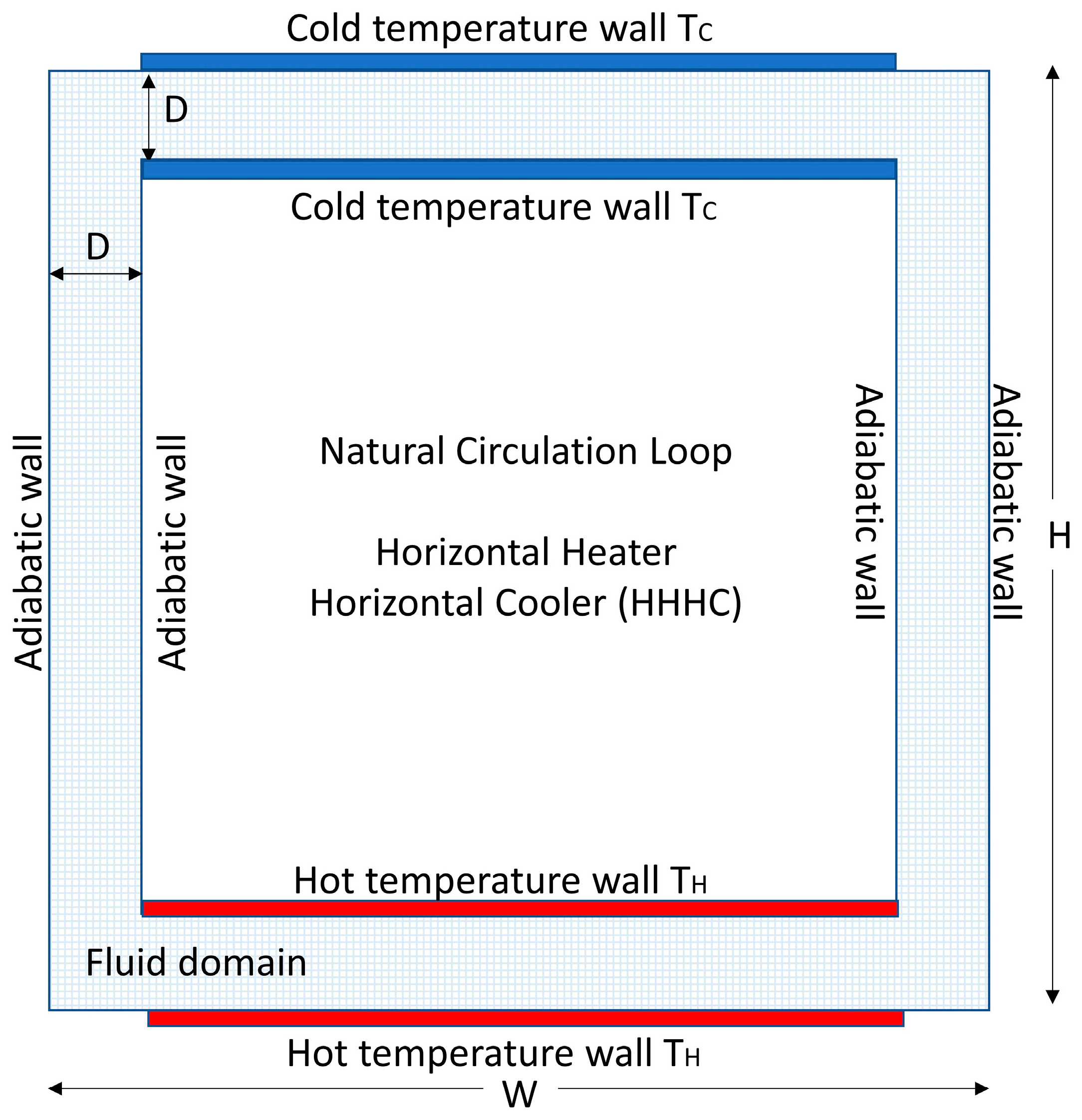
Figure 1 shows a schematic representation of the simulated loop and the main geometrical parameters considered. The width () and height () of the loop are set to the same value (0.250 m), while the internal tube diameter () is 0.010 m. The numerical model considers a square mini-loop with imposed heater and cooler temperatures ( and , respectively). The geometric proportions are similar to the experimental mini-loops researched in [4,7,8]. The heater and the heat sink are located in a horizontal configuration; this type of NCL is known as an HHHC (horizontal heater, horizontal cooler). The HHHC configuration is interesting because it is symmetric, both flow directions are possible (clockwise and anti-clockwise), and analytical expressions to validate the model results are available in the literature. Details about the LBM implementation are given in Section 2.1.
The Rayleigh number () was varied from 103 to 107 to observe the thermohydraulic behavior of the loop considering the velocity of the fluid into the channel (Reynolds number), the heat transfer characteristics (Nusselt number), and the thermal field (characterized by the temperature difference between the two vertical legs and the modified Grashof number). Even if the bulk results consider a computational fluid with a Prandtl number equal to one, some runs were made to observe the effect of changing the Prandtl number of the fluid.
2.1. Numerical Model Thermal Lattice Boltzmann Method
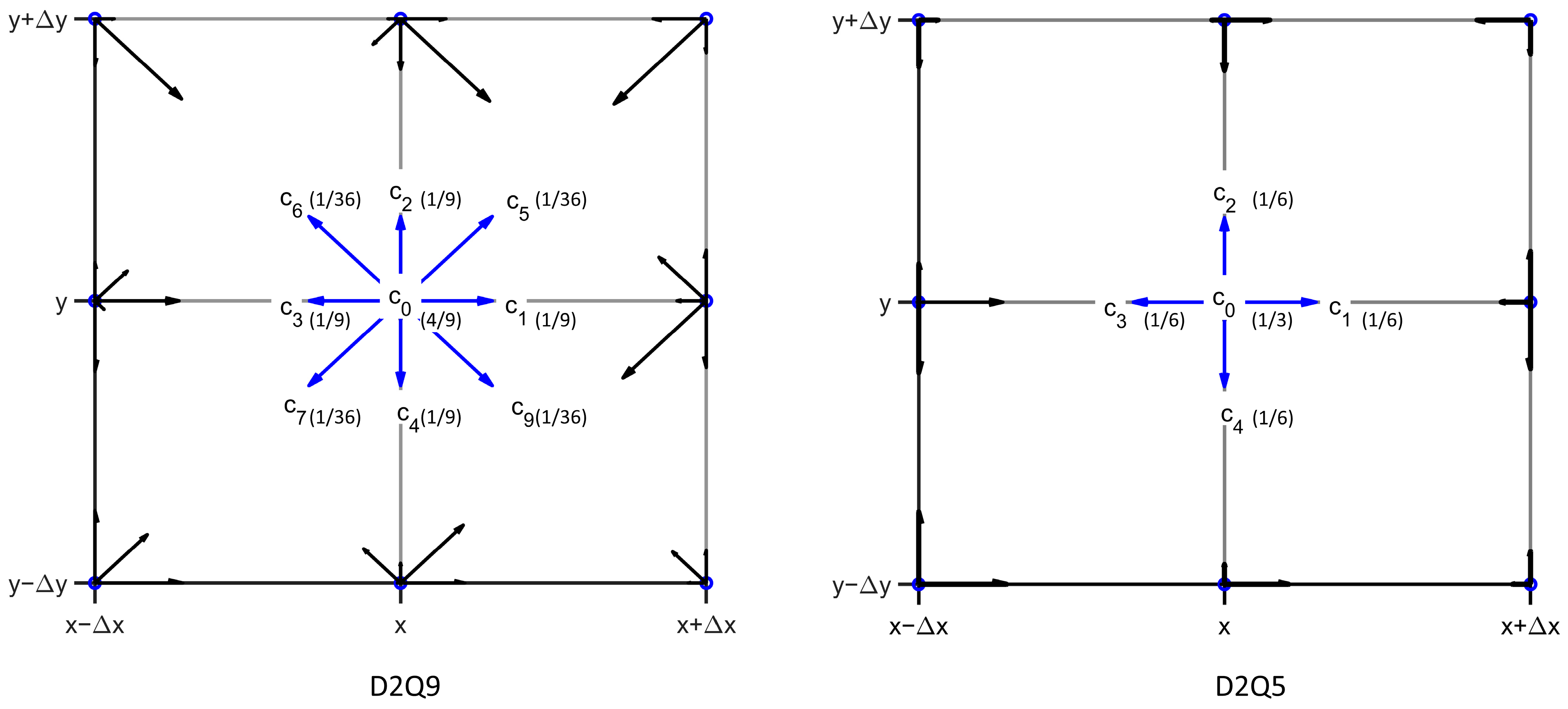
The geometry described in Figure 1 is modeled using a uniform square lattice. Multiblock allocation strategy is used to optimize memory usage, dividing the loop into four domains: heater, cooler, and the two adiabatic vertical legs A and B, i.e., the empty central nodes are excluded. The diameter is considered uniform along the two vertical legs, and cooler and heater sections. A bidimensional model of the HHHC single-phase NCL is implemented using the DDF approach proposed by He and Luo [44]. Figure 2 represents a D2Q9 lattice for the density and momentum field and a D2Q5 lattice for the temperature field. To obtain the target temperature field, it is enough to use the D2Q5 lattice, i.e., D2Q4 and D2Q9 give similar results, but the D2Q5 lattice is more stable [29]. In particular, the equilibrium distribution for both populations (density distribution functions) is Maxwellian and truncated to a second-order distribution (Taylor expansion), reproducing the conservation rules of mass, momentum, and thermal energy.
An alternative approach to thermal LBM simulations can be attempted by using a single multispeed lattice with a higher-order velocity discretization (e.g., D2Q17) that allows the calculation of higher-order moments. Note that the D2Q9 lattice is limited to second-order moments, and the third-order moment is necessary to obtain the energy field. Including additional velocity vectors adds complexity to the computational scheme; moreover, it breaks the algorithm’s local calculation property and degrades the LBM parallelism (one of the main advantages of using LBM). However, the multispeed approach can be suitable for Rayleigh Bernard’s natural convection simulations, including “viscous heating, heat conduction, and linear and non-linear acoustic effects” [45]. A second alternative for thermal LBM simulations is based on regularized schemes (i.e., equilibrium distribution function expanded to third-order) and non-Boussinesq approximations; this alternative has been recently developed [24] and tested with large temperature differences and Rayleigh numbers.
The general physical equations for the fluid are the Navier–Stokes equation, Equation (1), the continuity equation, Equation (2), and the temperature advection–diffusion or energy equation, Equation (3). In these equations represents the macroscopical velocity, the body-force term, the kinematic viscosity, the thermal conductivity, the fluid density, the temperature, and the time.
Instead of directly discretizing and simulating those equations, the LBM uses the discretized Lattice Boltzmann Equation (LBE) for the corresponding populations of the two lattices (local probability density functions and ). The LBE is presented in Equation (4) for the density-momentum, and Equation (5) for the energy field. The LBE represents a balance between the transport and collision processes between statistical distributions of the fluid molecules; the LBM is not a pure microscopic method (like simulating the dynamic of every single molecule) or a macroscopic method (considering the bulk fluid dynamics), and it is denoted as a mesoscopic method. Solving the LBE mesoscopic equations (Equations (4) and (5)) is analogous to solving the macroscopic fluid, Equations (1)–(3).
The LBE solution algorithm is divided into streaming and collision steps. The left-hand side of Equations (4) and (5), used for the streaming step, represents the transport of the populations between the nodes of the lattice at position and after each timestep . The right-hand side of these equations, used for the collision step, represents the collision process, which in this case, uses the BGK approximation that relaxes the population ( or ) to an equilibrium population ( or , respectively). The collision process is characterized by a relaxation time linked to the viscosity (Equation (6)) and a relaxation time linked to thermal diffusivity (Equation (7)). Additionally, the external force is included in the term and in our case represents the buoyancy force due to the thermal expansion of the fluid, meaning that this term is used to couple the two LBE equations.
The equilibrium function for the hydrodynamic field and the thermal field are presented in Equations (8) and Equation (9), respectively. The sound speed of each lattice is a propagation constant; for D2Q9 and D2Q5. Note that D2Q5 was selected to simulate the advection–diffusion of the thermal field due to its demonstrated robustness and accuracy compared to D2Q9 [30]. The velocity base and the corresponding weights for each lattice are presented in Figure 2.
For the thermal field, the equilibrium function couples with the hydrodynamic field through the velocity field . For a complete two-way physical coupling, the thermal field affects the hydrodynamic field by the force term in Equation (10). The Boussinesq hypothesis is used to model the force term (Equation (10)); a small change in the density has only an effect on the buoyancy force term, and thus it is possible to use a force term proportional to the temperature and control the strength of this effect by a proportional constant [25].
Macroscopic quantities are calculated using the integral moments of the density functions and . For the calculus of the density and momentum, the zero-order moment (Equation (11)) and first-order moments (Equation (12)) of are used, respectively. The temperature corresponds to the zero-order moment of (Equation (13)). The velocity field calculated from (Equation (12)) entered into Equation (9), and thus affecting the temperature distribution. On the other hand, the temperature affects the flux by calculating as presented in Equation (10) using the zero-order moment of previously used (Equation (13)) to calculate the thermal field ; through this interaction between both fields, the model can be considered two-way coupled. On the other hand, a single-way coupling can be used to simulate chemical species transport, i.e., the passive field (chemical species concentration) does not affect the flux.
The described model is suitable for low-Reynolds-number thermal flow simulations. Under some conditions, such as reducing the Prandtl number, the Reynolds number can be over 1000, generating convergence issues. However, considering the validation data and relationships reported by [3], the range of interest for this work remains in the low-Reynolds-number zone, and viscosity filters or other turbulence models are not necessary.
2.2. Boundary Conditions
A non-slip boundary condition (bounce-back) was implemented along all the loop walls for the hydrodynamic distribution. This boundary condition simulates a wall halfway between the wet and solid nodes. The implementation is simple, and the algorithm reflects the upcoming populations to the wall [46]. The behavior of this kind of BC induces the parabolic Poiseuille velocity profile at a low Reynolds number—a laminar regime.
The boundary conditions for the temperature field are composed of adiabatic walls at the vertical legs and fixed temperature walls at the heater and heat sink. The adiabatic condition is achieved by extrapolating the temperature in the neighbor nodes to remove the temperature gradient at the wall. The constant temperature boundary condition at the cooler and heater constitutes a Dirichlet-type boundary condition for the secondary (or thermal) distribution. The Dirichlet boundary condition was used to impose a fixed temperature on the corresponding walls of the simulation domain. Specifically, it ensures that the sum of the distribution functions () equals the desired temperature (). Depending on node positions, certain values of the probability density function could be determined during the streaming step. Subsequently, the remaining population values can be calculated using the equilibrium distributions by applying flux conservation principles. For further information on this implementation, we refer readers to [28,47] for more comprehensive details and insights. Some other possible schemes have been recently proposed to implement such boundary conditions using a single-node approach for the treatment of curved boundaries [48]; however, evaluating the accuracy or stability of these alternative boundary condition is beyond the scope of this study.
2.3. Initial Condition
A uniform density was established for all the computational domains. The LBM operates under the assumption of small density variations within the incompressible regime.
The initial velocity field can be established as zero, and after some time, the symmetry breaks, and the fluid starts to flow in one direction (either clockwise or counterclockwise). Alternatively, an initial low-velocity field can establish a flow direction and accelerate the convergence to the steady state.
The initial temperature field can be established using various approaches:
- Set the cooler temperature for all the domains.
- Set a temperature average for all domains.
- Set the heater temperature for the heater pipe, the cooler temperature for the cooler pipe, and a gradient field in the vertical legs.
The first two options are useful for testing the thermal boundary conditions at the cooler and heater; meanwhile, the third option reduces the convergence time to a steady state. The second condition was selected to perform the simulations. The thermohydraulic behavior at the steady state under the three listed initial conditions is analogous. Eventually, all the conditions converge to the same steady state. Consequently, the choice of the initial condition exerted minimal influence on the overall findings presented in this study.
To control the main fluid flow direction, three distinct strategies can be implemented:
- Introduce a slight offset in positioning the heater (or cooler) to disrupt loop symmetry.
- Create an initial temperature difference between the vertical legs.
- Impose a small initial velocity in a specific direction.
The third condition was adopted to conduct the numerical experiments. All three strategies were tested, successfully establishing a preferred flow direction. However, it is interesting to note that the third strategy does not alter the loop symmetry. Indeed, both flow directions remain possible. In particular, for high Rayleigh numbers, circulation occurs in both directions due to the initial fluid circulation complexity. The modest initial velocity does not necessarily fix the flow direction.
2.4. Units
The correspondence between computational units, also named Lattice Units (LU), and physical units in LBM is not straightforward. The difficulty in establishing a correspondence is because the computational length and time scales are linked through the relaxation parameter, including an additional free parameter into the unit conversion; conversion factors between the lattice units and the physical units must be carefully adopted. A different approach, based on normalized quantities and dimensionless groups, was adopted; in this way, the LBM results and the physical units are directly comparable [49].
The following quantities were considered in the physical analysis: The temperature normalization is implemented using for the heater and for the heat sink [50]. A given Prandtl () number characterizes the fluid in the loop. The ratio between the momentum (Equation (6)) and thermal diffusivity (Equation (7)) in the implemented LBM can be expressed as shown in Equation (14) to define .
The Reynolds number at steady state , Equation (15), is referenced to the pipe diameter and a representative velocity of the fluid in the loop named (representing the root mean square velocity in the cross-section of the pipes).
Rayleigh number (Ra), Equation (16), is referred to the temperature difference between the heat source and the heat sink , the vertical height of the loop , the gravity and the thermophysical properties of the fluid ( coefficient of expansion, thermal conductivity, and fluid viscosity). is an input parameter that is fixed before the simulation starts.
Modified Grashof number is defined in Equation (17). Note that this number differs from the Grashof number defined in Equation (16) because it considers the average temperature difference between the hot and cold legs () as the thermal gradient that determines the thermohydraulic behavior and considers the pipe diameter as a relevant characteristic dimension. However, this number cannot be determined a priori but can be determined after the steady state is reached, performing an average on the thermal field of each vertical leg.
The local Nusselt number , Equation (18), and average Nusselt number , Equation (19), can be evaluated utilizing the gradient of the thermal field.
Considering M, the number of lattice nodes in the heater direction, the wall temperature , the neighbor nodes temperature and , and N number of cells in the perpendicular direction y. is calculated by a first-order finite difference scheme FD1 (Equation (20)) or a more accurate second-order scheme FD2 approximation (Equation (21)).
2.5. Stability and Convergence
The convergence of the system to the steady state is determined by calculating when the relative standard deviation of the Nusselt number is below a given threshold (up to 10−16). When this condition is reached, the simulation is finished. Additionally, the convergence of the temperature difference between the hot and cold legs () and Reynolds number was studied. In the laminar regime, these quantities converge. The simulations do not present computational instabilities or divergences in the tested Rayleigh number range.
The resolution effects on flow conditions were investigated, calculating under the same operation conditions. The following spatial resolution values were tested: 500 (diverge), 1000, 2000, 4000, 8000, and 10,000 grid points per meter. It was noted that converges for a resolution up to 4000; thus, 40 mesh points per pipe diameter were used in the simulations, i.e., 1000 × 1000 lattice.
During the simulations, the relaxation time of each lattice (fluid and thermal) were adjusted to obtain the desired Prandtl number. Some important parameters are listed in Table 1, including imposed global Rayleigh number (, the imposed temperature difference between heater and heat sink (), geometric ratios such as diameter to total loop length () and width to height ratio (), viscosity () and thermal diffusivity (), reference velocity (), and Prandtl number; these values were adjusted to obtain feasible results and ensure convergency and stability. It is important to note that the optimal parameter selection may vary depending on the specific flow scenario and research objectives. A combination of physical insights, numerical stability considerations, and validation against experimental or analytical results is typically employed to ensure accurate and reliable simulations [46,47,49]. The main considerations that provide a framework for selecting parameters in Lattice Boltzmann simulations are based on the physical considerations (to simulate a desired phenomenon adequately), grid resolution (to resolve relevant length scales), lattice model, relaxation time (to adjust the velocity of the distribution function to approximate the equilibrium distribution), boundary conditions (such as non-slip walls or adiabatic or thermal walls), time step (small enough to capture flow features), and finally, the validation method (contrasting the simulations with experimental or analytical results).
2.6. Computational Considerations
The NCL model was implemented in C++ using the parallel Lattice Boltzmann library PALABOS [51]. The routine was tested in an Intel® Xeon® Platinum 8260 CPU, 2.40 GHz, workstation, using an MPI (message passing interface) protocol for the parallel running on 48 cores. The maximum calculus velocity was approximately 250 MSUPS (Mega Site Updates Per Second) for a resolution of 10,000 grid points/m and 200 MSUPS for the simulations with 4000 grid points/m.
3. Results
3.1. Laminar Regime
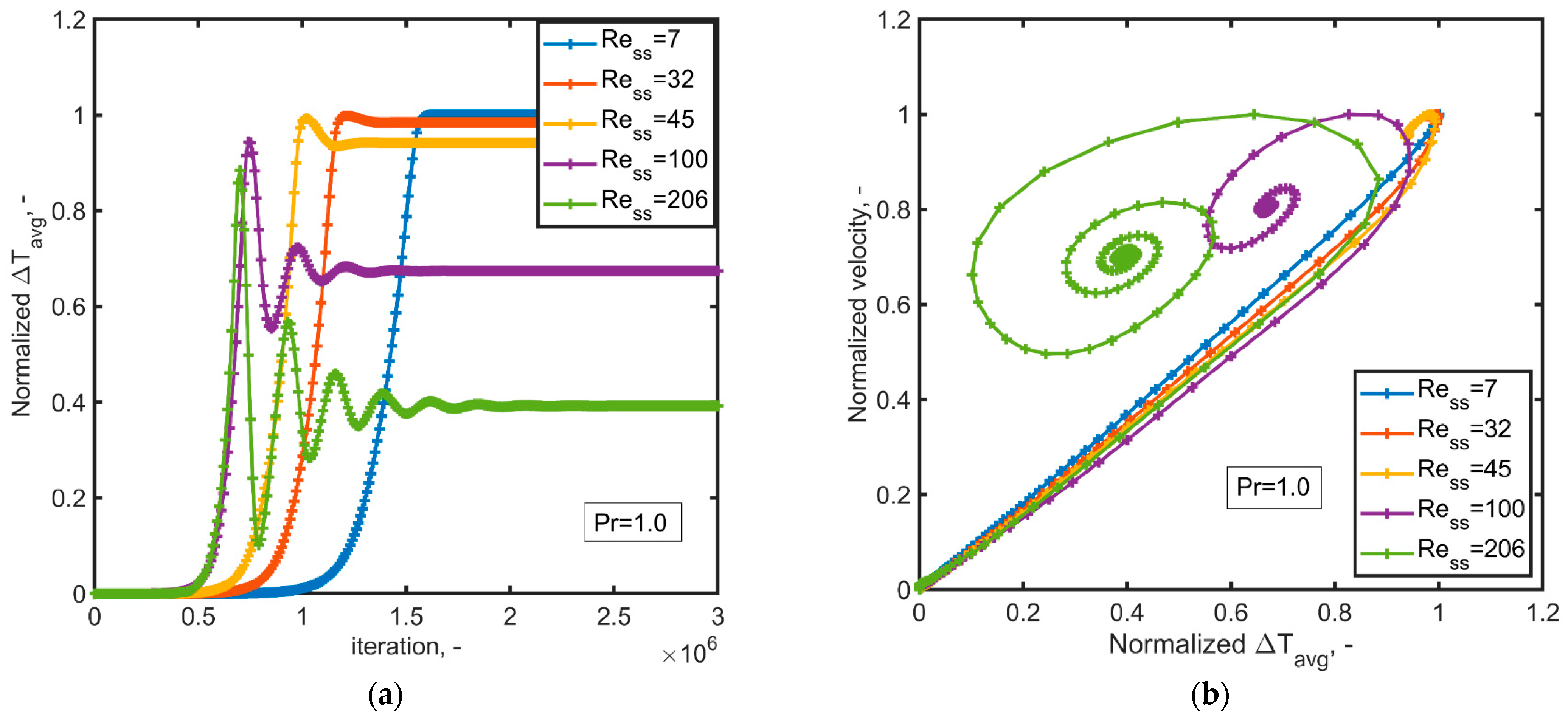
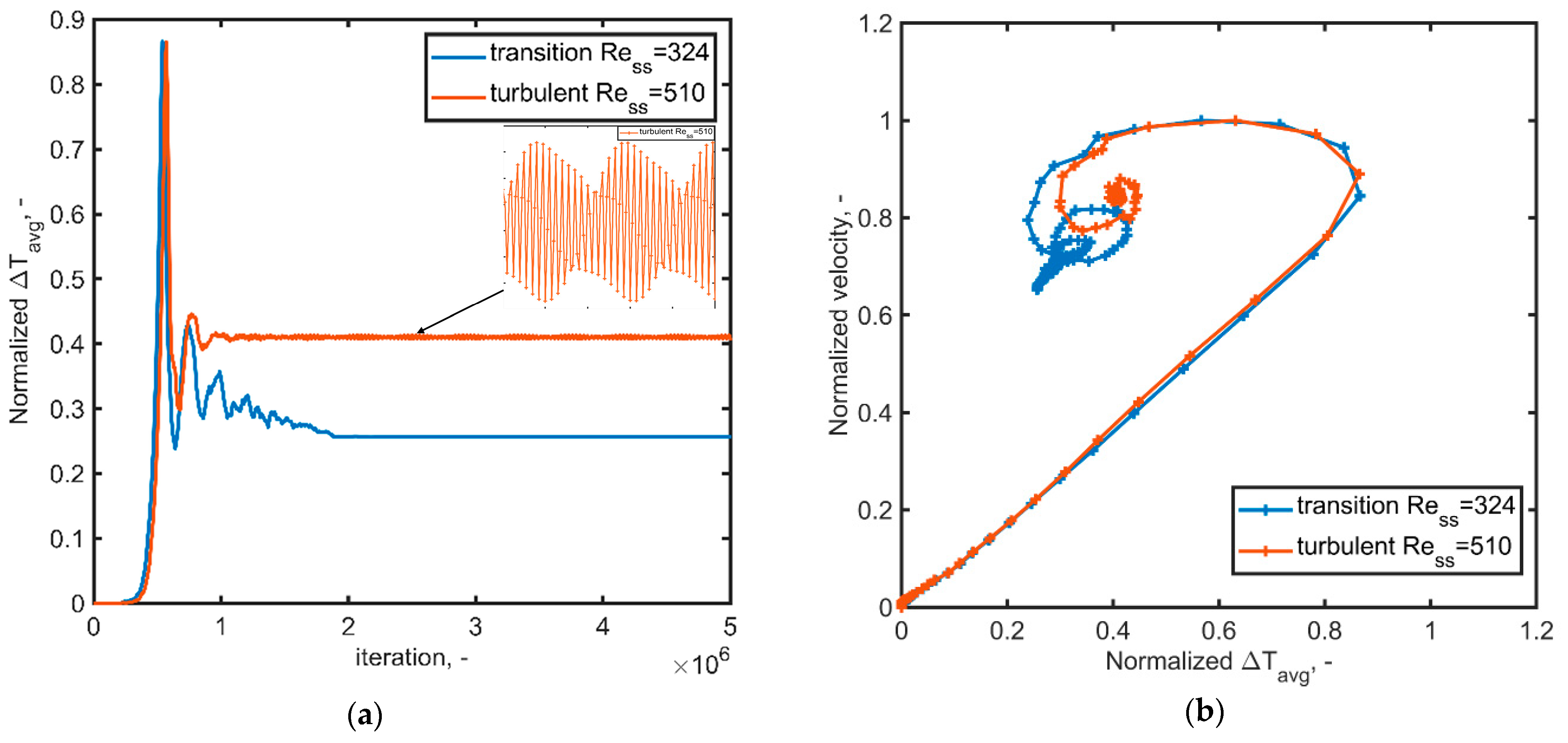
The convergence to the steady state of the circuit is illustrated in Figure 3a. This figure presents the normalized temperature difference between the adiabatic vertical legs at different time step iterations. For higher (and ) values, the time from the rest state to the onset of natural convection was shorter, and the achieved normalized temperature difference between the legs decreased. The transient stage exhibits fewer oscillations for low (and ) due to the slower fluid motion, allowing the heater and cooler to more effectively alter the fluid temperature during its circulation. This pattern aligns with the findings of Cheng et al. [4], even though their work presents an “absolute” increment of . Moreover, the transient behavior aligns with previous findings by Garibaldi and Misale [52] for mini loops with small inner diameters: the amplitude of oscillations increases with higher heating power. As highlighted in [8], the efficiency decreases with an increase in the Rayleigh number. Figure 3b presents a phase diagram comparing the simultaneous convergence of the temperature difference and velocity. Notably, an increase in the phase difference between velocity and temperature oscillations was observed for higher Reynolds numbers.
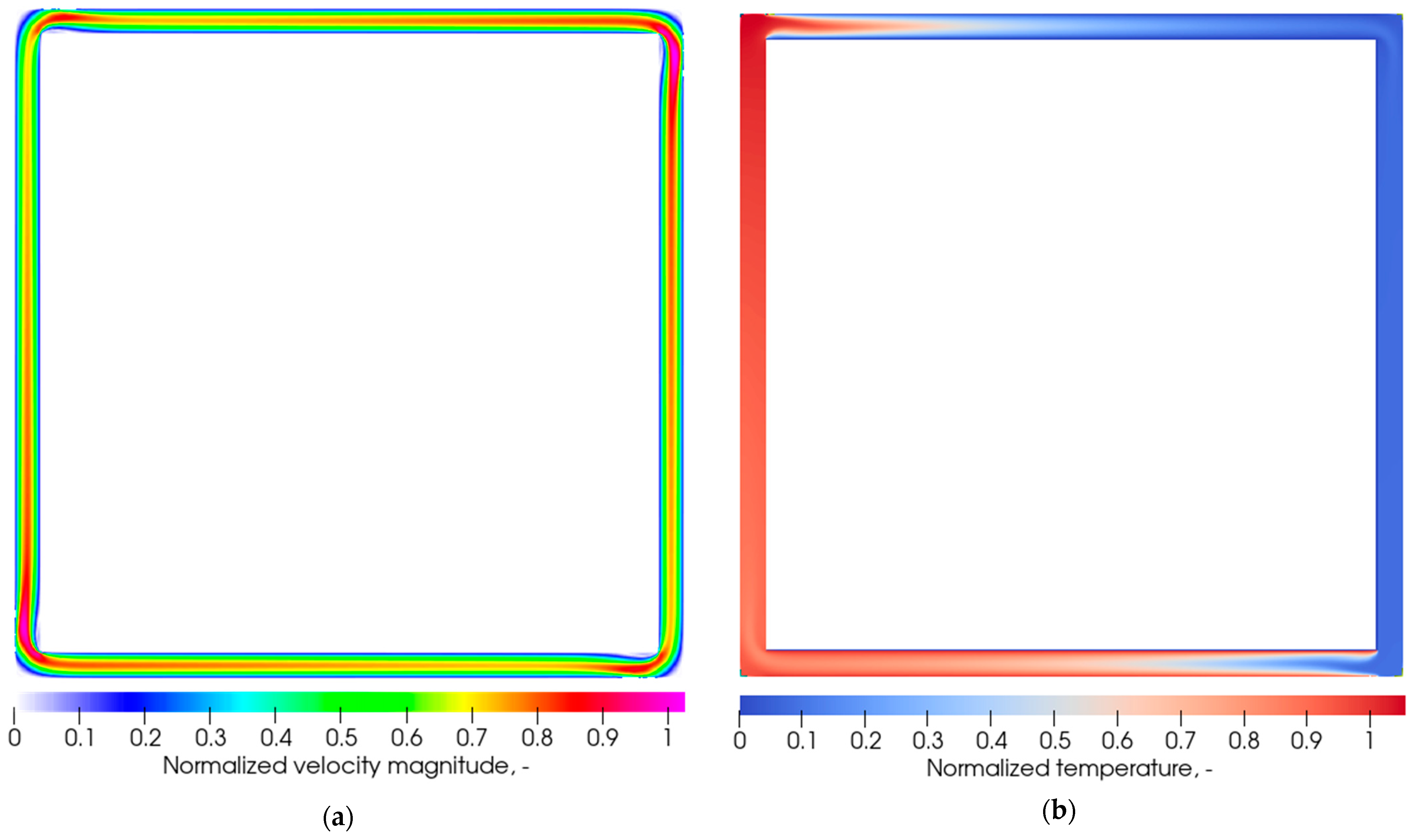
Figure 4a depicts the characteristic behavior of the NCL at a low Reynolds number (). The cross-sectional velocity field was characterized by a parabolic profile, devoid of vorticity. The temperature field presented in Figure 4b exhibited minimal temperature variation along the vertical legs. As was expected, the fluid temperature increased in the heater and decreased in the heat sink.
The current LBM approach is validated using the model proposed by Cheng et al. [4] for a single-phase NCL with fixed temperatures at the heat sink and heat source. This Cheng et al. model has been experimentally corroborated for Reynolds numbers below 100 () [4]. Built on a one-dimensional analysis of the loop in the laminar regime, the model employs the Boussinesq approximation to account for buoyancy effects arising from the fluid’s thermal expansion. It does not incorporate axial heat conduction, viscous dissipation, or changes in fluid physical properties due to temperature effects. Both heat source and heat sink temperatures are held constant. Under these premises, they derived the relationship presented in Equation (22) for the Reynolds number at steady state and the modified Grashof number (Equation (17)) and the dimensionless geometrical factor that accounts for frictional effects, as outlined in Equation (23). Importantly, it is possible to show that this model is equivalent to the model proposed in [3,17] in an NCL with a heat flux boundary condition at the heater.
The geometrical parameter accounts for local and concentrated losses considering the frictional coefficient (calculated using ) and the local resistance coefficient .
The LBM results reproduced the theoretical model for low Reynolds numbers [43]. The LBM results for high Reynolds numbers show a small deviation from Equation (22).
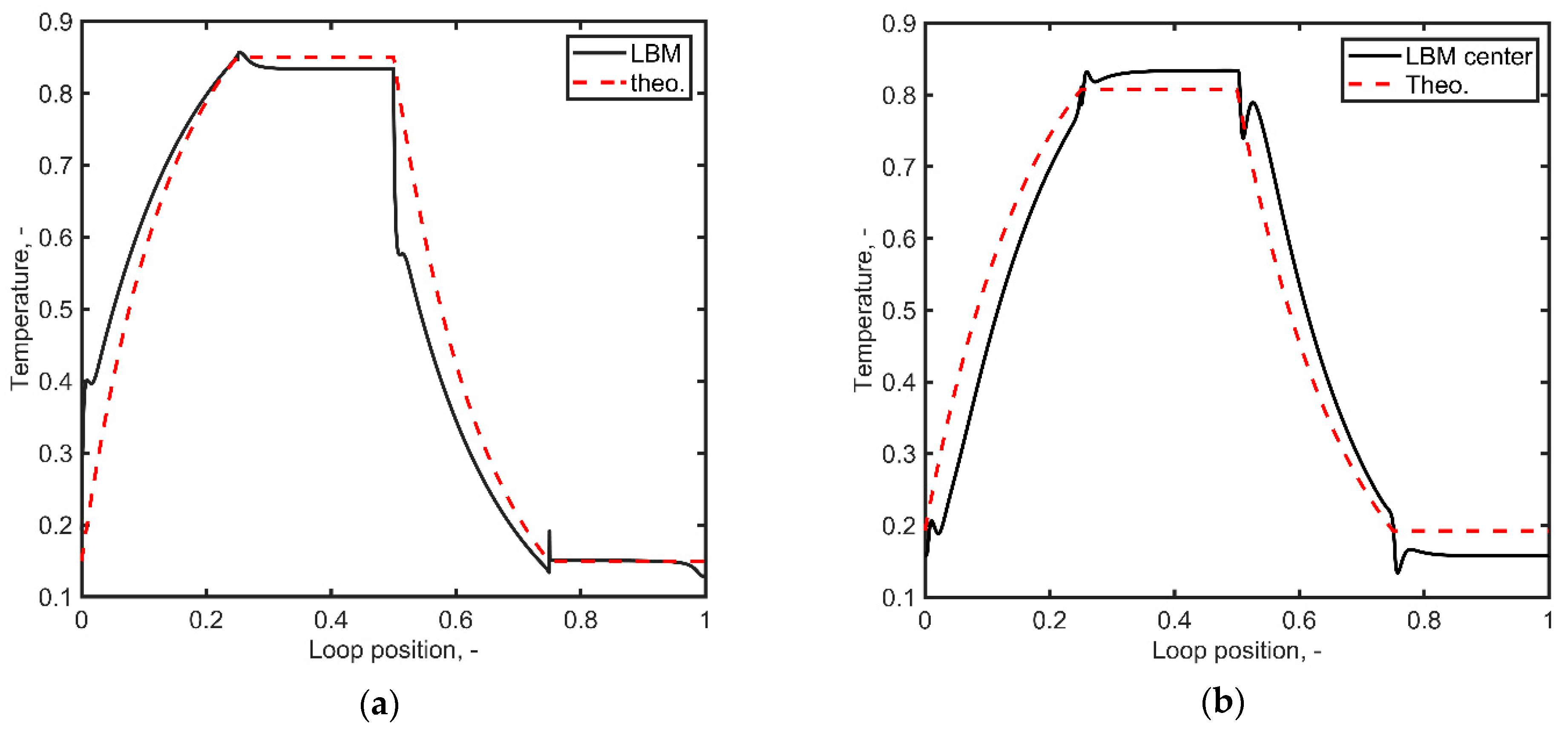
The analytical model allows for temperature calculations for each section of the circuit. Figure 5 displays a comparison between the one-dimensional theoretical model and the LBM results, focusing on low Reynolds numbers indicative of the laminar regime. It is important to observe that Figure 5 delineates four distinct sections correlating with the normalized loop position axis, specifically the vertical leg A (from 0 to 0.25), heater (from 0.25 to 0.50), vertical leg B (from 0.50 to 0.75), and cooler (from 0.75 to 1). Figure 5a showcases the average temperature of each cross-section, while Figure 5b illustrates the temperature at the center of the tube. Both the one-dimensional and LBM outcomes exhibit a similar shape, yet certain differences arise, particularly when evaluating the average temperature of each cross-section, i.e., these differences were less pronounced when the temperature at the center of the tube was considered. The contrast between the center temperature and the cross-sectional average indicates the significance of the axial temperature distribution, predominantly in the initial portion of each pipe. The diffusion of the temperature field contributes to a more uniform temperature profile, with a smaller effect on the longitudinal temperature profile. The theoretical model results depicted in Figure 5 were presented in detail in [4], where dimensionless temperature distributions were derived based on the governing equations for the heater, pipes, and cooler under steady state conditions. The temperature distribution within the vertical legs follows an exponential form.
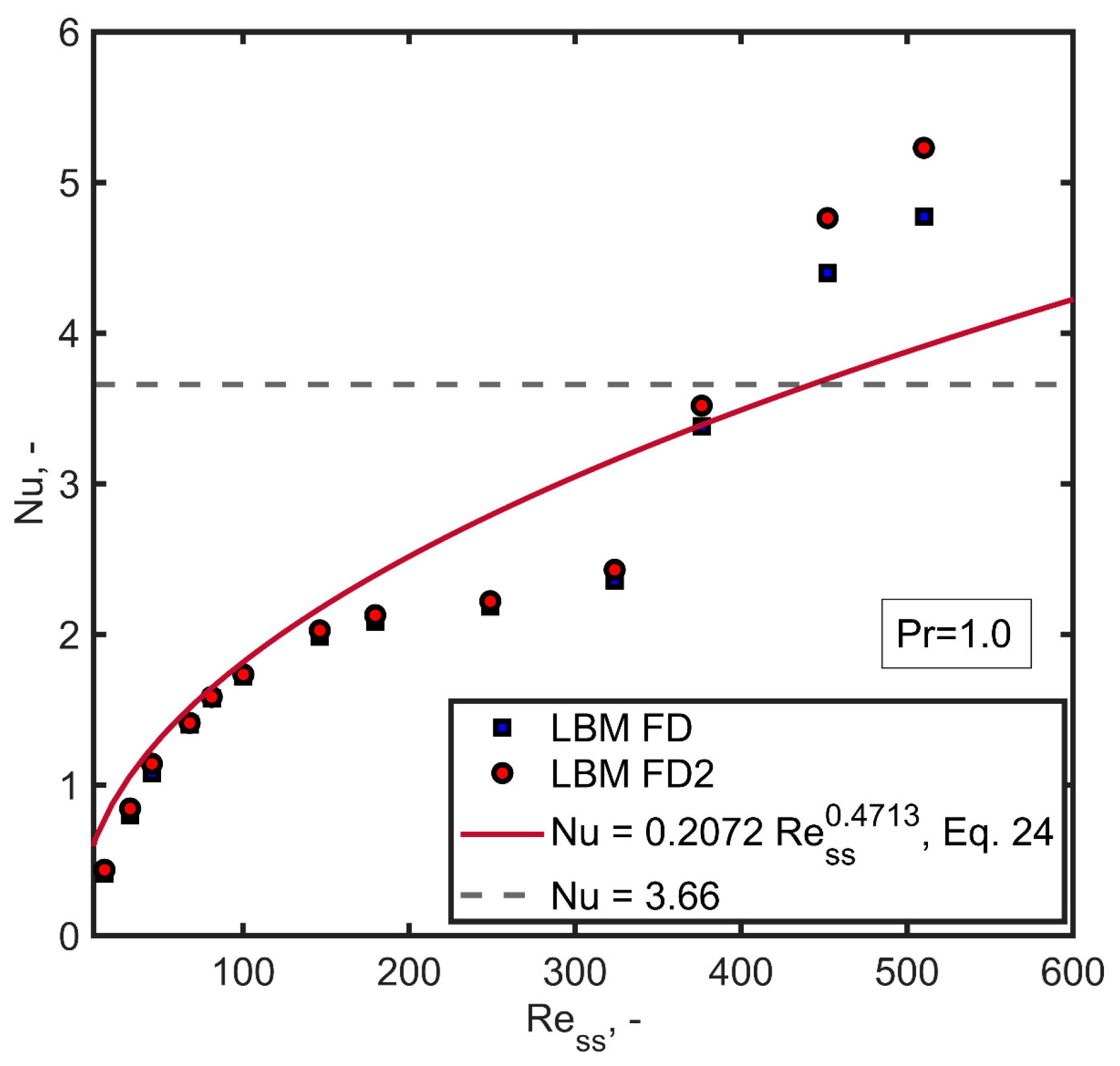
The Nusselt (Nu) number is used to describe convective heat transfer characteristics of the system. The computation of the average Nusselt number along the heater through LBM involves the utilization of Equation (20) (FD) or Equation (21) (FD2). Figure 6 provides a comparative analysis between the computed average Nusselt number along the heater and the empirical correlation proposed by Cheng et al. as outlined in Equation (24) [4]. Clearly, the commonly accepted simplistic expression for the heat transfer of a developed (laminar) flow in a pipe fails to capture the heat transfer characteristics along the loop. Both the empirical equation and the simulations underscore that the heat transfer exhibits lower values (below 3.66) within the laminar regime, which subsequently amplifies with the Reynolds number while showcasing a non-linear dependency.
The observed discrepancy between Equation (24) and the numerical outcomes underscores the pronounced influence of the fluid dynamic regime on convective heat transfer; note the sudden increase in the Nusselt number for a . While Equation (24) is based on empirical data derived from laminar flow conditions, it might not comprehensively capture the convective heat transfer trends observed in our numerical simulations where the fluid flow potentially undergoes a transition to a turbulent regime. In turbulent flow, recirculation and complex flow patterns enhance convective heat transfer due to increased fluid mixing and motion, resulting in higher heat transfer rates compared to laminar flow. Future investigations will focus on incorporating turbulence models and conducting experimental studies to validate the numerical results under transition and turbulent flow conditions and gain deeper insights into the distinct flow regimes.
The LBM results align with Equation (24) for Reynolds numbers below 200. From this threshold up to the critical Reynolds number that determines the transition to non-laminar flow ( around 320), the exponent of Equation (24) experienced a decline. Subsequently, a distinct Nusselt number correlation emerged, characterized by a more substantial increase.
3.2. Transition to a Non-Laminar Regime
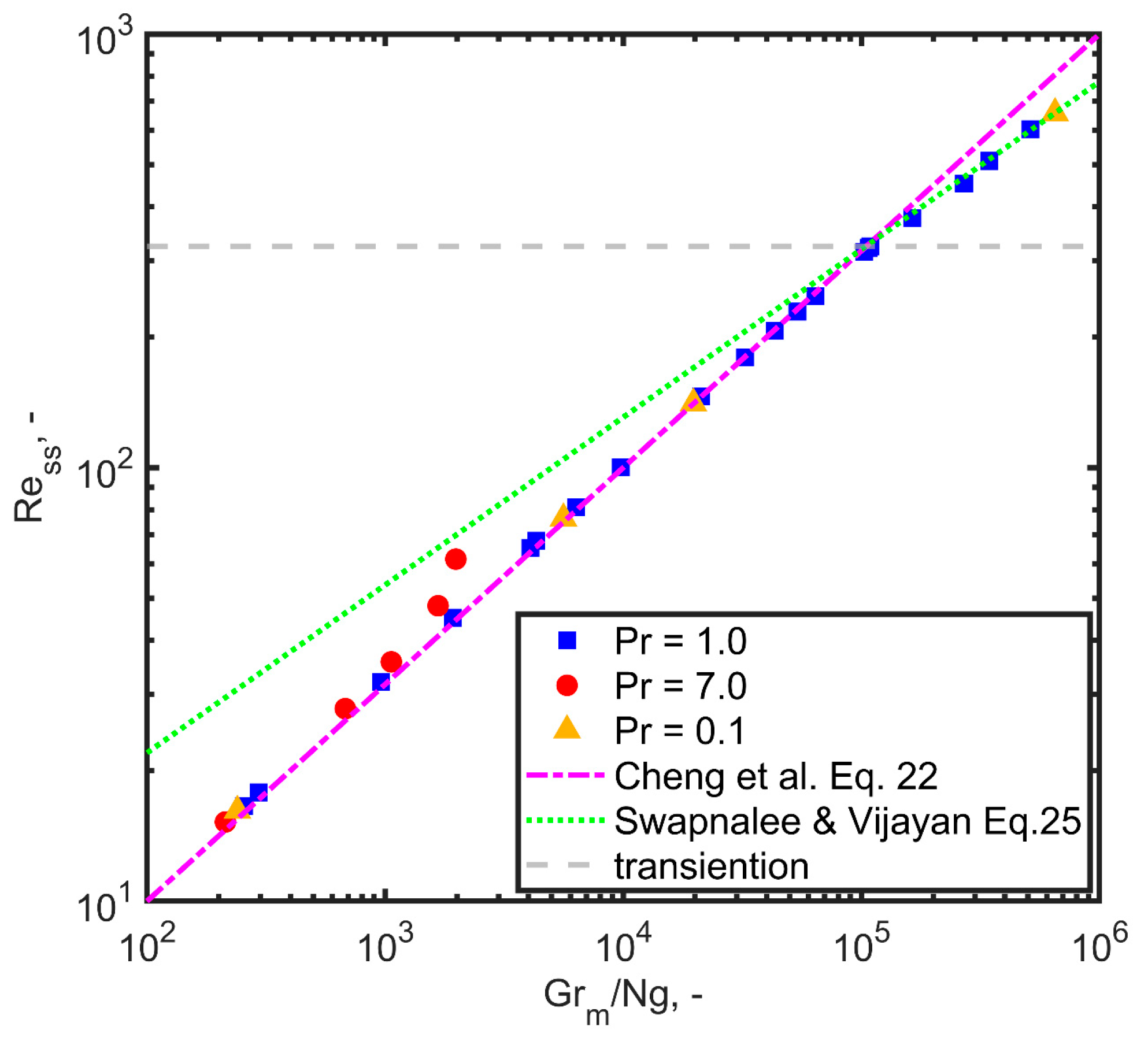
The applicability of the theoretical model (Equation (22)) is confined to the laminar regime. However, our investigation revealed the emergence of a non-laminar flow pattern for values of around 105, equivalent to a steady state Reynolds number () of around 320. This transition is evident in the logarithmic chart depicted in Figure 7, where there was a noticeable alteration in the slope close to this threshold (). It is important to observe that this change in slope correlates with the sudden increase in the Nusselt number exhibited in Figure 6.
The transitions region in closed loops with the HHHC configuration is expected to occur at Reynolds number values lower than the accepted threshold for straight pipes, as noted by various authors, including Creveling et al. [53] (), Hallinan and Viskanta [54] (), and Swapnalee and Vijayan [3] (). These latter scholars proposed an alternative friction factor, characterized by for the turbulent regime, and for the transition regime. Incorporating this friction law leads to a change in the exponent within Equation (22), as demonstrated in Equation (25). The rationale underlying the adoption of this friction law for the transition regime is shown in Figure 7.
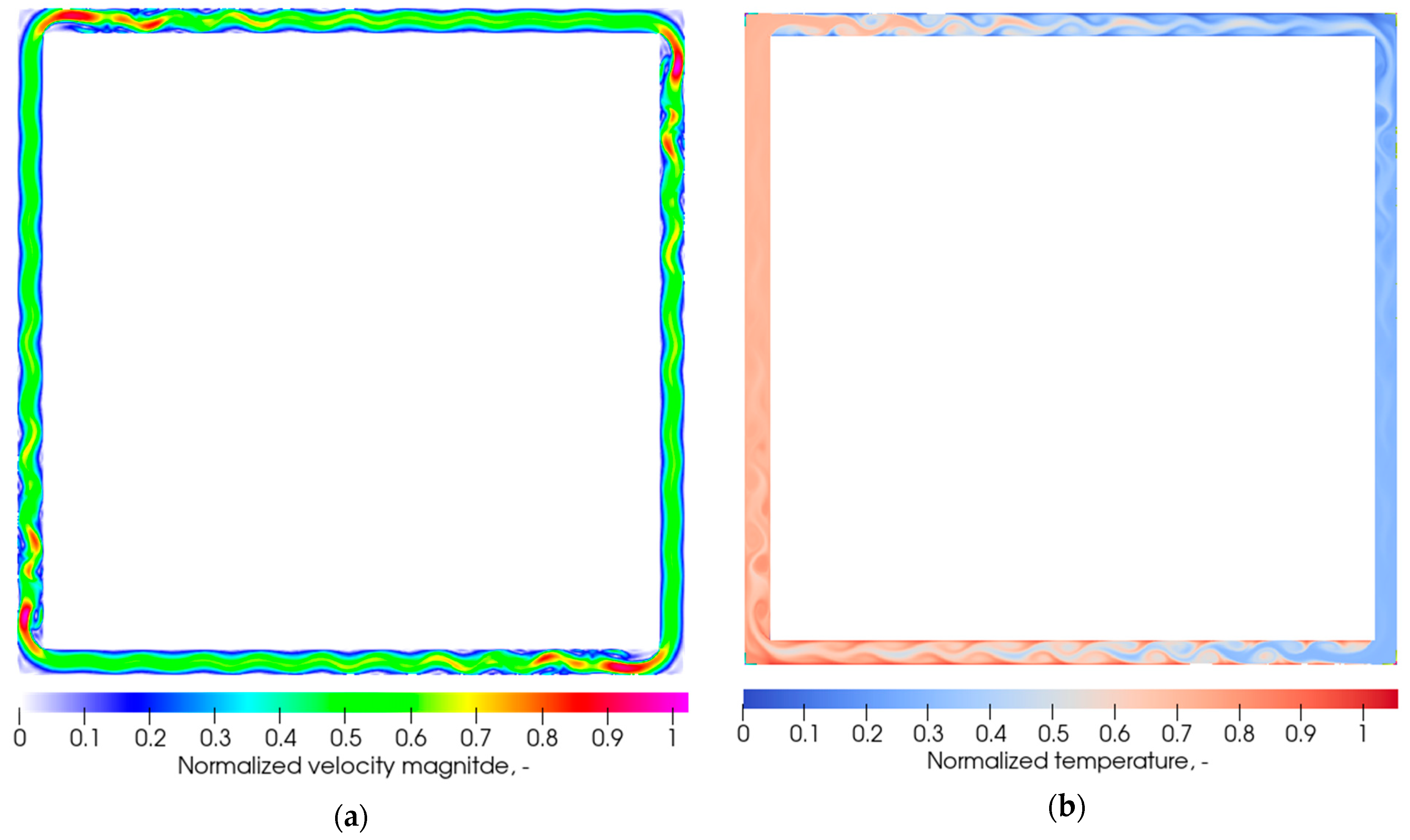
The transition in the flow regime becomes evident in the velocity and thermal fields, as illustrated in Figure 8. This transition was characterized by vortices forming near the walls, which enhances convective heat transfer by facilitating fluid recirculation along the heater and heat sink pipes. These vortices traveled in the same direction as the mean flux and remained near the walls. Additionally, a discernible alteration was observed in the transient response of the circuit. Figure 9 depicts an example of the transient temperature response near the threshold of the transition regime () and the non-laminar regime (). During the temperature oscillations near the transition regime threshold, certain eddies became visible; however, the system eventually reached a steady state characterized by laminar flow after a certain period.
Conversely, for higher Reynolds numbers, the system did not reach a true steady state condition; instead, temperature oscillations persisted around a central value, as shown in Figure 9. A detail of this pseudo-steady state behavior is provided in the figure. The flow and thermal pattern remained consistent with those depicted in Figure 8. Lastly, the phase diagrams in Figure 9b detail these two examples. In the case of , the system experienced an abrupt change in dynamics after a series of oscillations, eventually converging to a steady state. In contrast, at , the slight oscillations around the pseudo-steady state temperature induced corresponding fluctuations in the velocity flow.
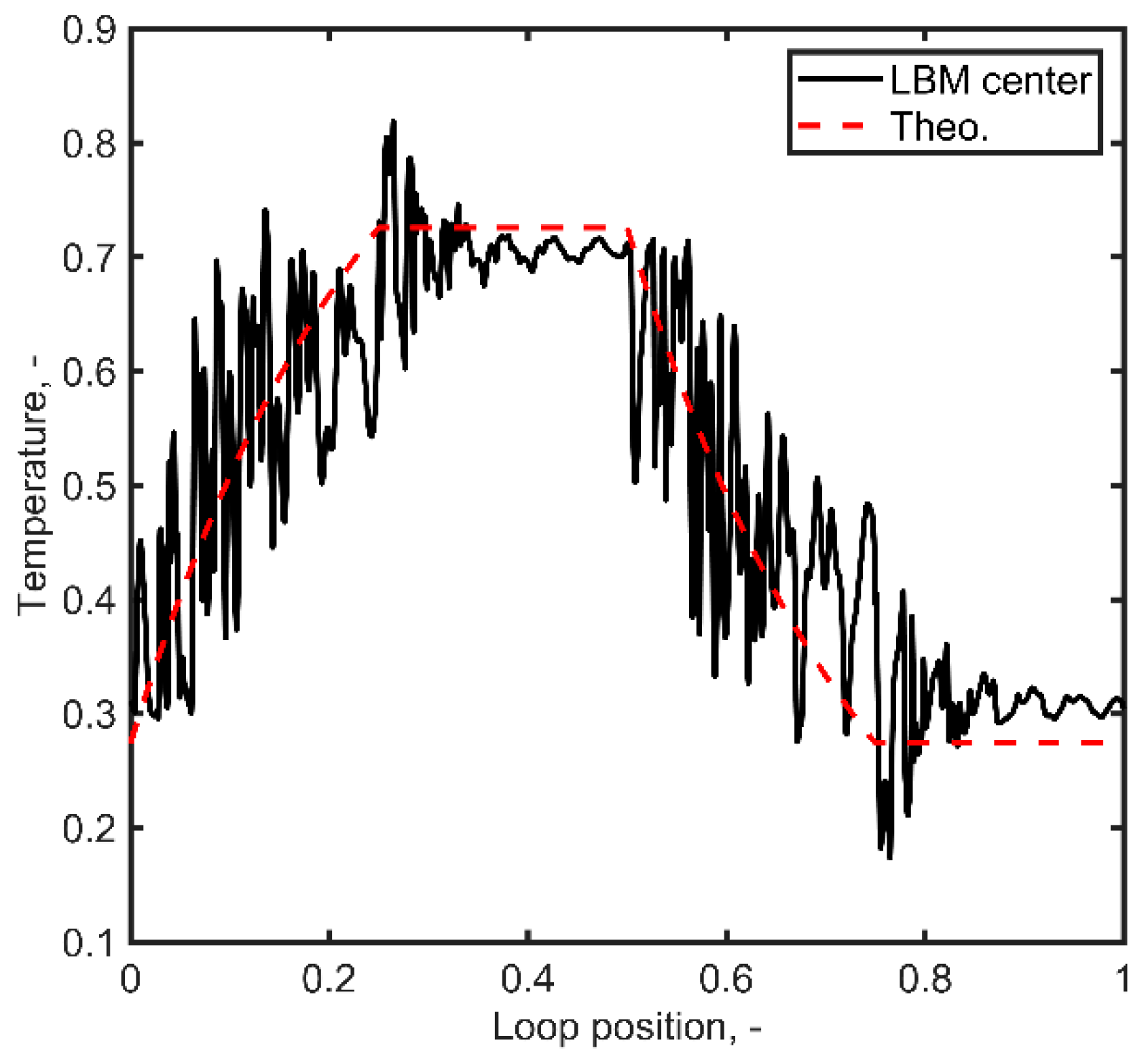
The presence of vorticity significantly influenced the temperature distribution along the circuit, particularly in the non-laminar regime near the walls of the heater and heat sink, as well as in the initial section of the vertical legs (see Figure 10). The temperature profile at the center of the tube exhibited substantial oscillations. Notably, the temperature profile predicted by the one-dimensional model only loosely resembled the LBM results. This discrepancy might be attributed to vorticity, a three-dimensional phenomenon that cannot be adequately captured within the constraints of a one-dimensional model. Our 2D approach, as observed, effectively captured the principal characteristics of the one-dimensional model proposed in [4], particularly under steady state conditions and laminar flow. The transition to non-laminar flow triggered a noticeable alteration in the friction factor, as suggested in [3]. This agreement between our simulation outcomes and the established one-dimensional model reaffirms the accuracy and reliability of our 2D approach in replicating the fundamental traits of the system in laminar flow conditions. This underscores the robustness of our computational methodology in modeling the thermohydraulic behavior of the single-phase NCL. However, we acknowledge the necessity for further investigation and refinements to address the limitations, including aspects like fluid selection and 3D modeling, to more accurately represent real-world scenarios and explore the transition to turbulent flow.
The occurrence of this non-laminar regime at a relatively low Reynolds number, which is below the conventionally accepted critical values of 2000 for transition and 2300 for the turbulent regime, remains unknown, and more research is necessary to probe if it is a physical phenomenon or is solely a numerical artifact. Nevertheless, several hypotheses that potentially elucidate this behavior include the following:
- The presence of acute bends and corners in the geometry could introduce flow obstacles that trigger the observed deviations from laminar behavior.
- The simplified geometrical model might induce local pipe diameter changes at corners, potentially causing fluid expansion and contraction and consequently influencing the flow pattern.
- Fluid acceleration induced by the Boussinesq force, particularly at the heater and heat sink, could contribute to altering the flow characteristics.
- Furthermore, the presence of vorticity, a fundamentally three-dimensional phenomenon, might be roughly approximated using the bidimensional model employed in this study.
Addressing the underlying causes of this non-laminar regime deserves further investigation and may shed light on whether these hypothesized factors contribute to the observed behavior or if other mechanisms are at play.
The number of mesh points used in the simulations (40 along the pipe diameter) may prove insufficient to fully capture the boundary layer, particularly during the transition regime for high Reynolds numbers. Nevertheless, for the laminar regime, the convergence of the results with this mesh resolution was observed, and the cross-sectional velocity profile exhibited a parabolic profile, indicating a developed flow with a boundary layer near half the pipe diameter. However, the results for the transition region, where turbulence was observed, may be under-resolved. It is well-known that turbulence is inherently a three-dimensional phenomenon that two-dimensional or one-dimensional models do not adequately describe. Hence, our findings should be considered as an initial numerical approximation that attest to the presence of a laminar flow limit and the existence of a transition regime. Future studies should incorporate three-dimensional models, coupled with adaptive LBM stencil strategies near the walls, incorporation of turbulence models, and experimentation with different fluids to reproduce the transition regime in the laboratory. The need to refine the LBM numerical approach emerges from the previous considerations, with the imperative for accurate three-dimensional models featuring a high mesh resolution to capture minute turbulences. Of course, the computational load increases considerably with those LBM upgrades.
It is necessary to consider that the presence of eddies does not inherently indicate a fully turbulent regime, with the subsequent energy cascade from the large eddies to the small ones. Indeed, our results do not invalidate the applicability ranges of Equation (22). Instead, our results underline the importance of conducting experiments at higher Reynolds values. This presents a challenge, as reaching and maintaining single-phase conditions at high Rayleigh numbers is intricate. Selecting an adequate working fluid, characterized by a low Prandtl number, might be a viable strategy to overcome this hurdle and extend the exploration into higher Reynolds regimes. A notable limitation of this study involves the selection and modeling of the working fluids. In most cases, a Prandtl value of was employed, which is indeed close to the value of air () and may not be representative of practical applications scenarios. To address this concern, we have included supplementary outcomes using to investigate the impact of a higher Prandtl number. As a result, the selected values encompass fluids of interest, such as water or molten salts. However, further studies should explore a broader range of Prandtl number values relevant to specific applications. The limitations associated with fluid selection and the use of fixed thermophysical properties are acknowledged, emphasizing the importance of considering more comprehensive fluid models and varying Prandtl numbers to enhance the applicability of the results. This study will pave the way for future research exploring a wider range of Prandtl numbers for greater realism and applicability.
Utilizing the LBM in this study provides valuable contributions and insights that complement previous research on NCLs. Its parallelization capabilities, direct temporal convergence, ability to handle coupled fluid flow and heat transfer, and capturing complex flow phenomena all contribute to a more comprehensive understanding of the system’s behavior. The study of this kind of system using LBM enhances the existing knowledge in the field and offers a unique perspective on the thermohydraulic behavior of NCLs. Moreover, future studies could benefit from implementing a multi-physics LBM simulation that includes, in addition to the present model, a coupled lattice representing a secondary species dispersal (i.e., nanoparticles) and possible sedimentation during the NCL operation.
The practical relevance of this research lies in developing valuable simulation tools to analyze and predict the behavior of single-phase NCLs under various operational conditions. The accurate representation of the thermohydraulic characteristics of NCLs through our 2D approach can be a useful tool for engineers and researchers in the field. By simulating the fluid dynamics and heat transfer phenomena within the loop, our model enables the evaluation of different operating scenarios and optimizing system performance without the need for costly and time-consuming experimental setups. Moreover, our results open avenues for further research that could enhance the practical applications of NCLs. Future studies may explore complex geometries, different working fluids, or even the inclusion of nanoparticle dispersions for advanced heat transfer applications.
4. Conclusions
In this study, a bi-dimensional Lattice Boltzmann Model based on double distribution functions was developed to simulate a square single-phase natural circulation loop with fixed temperatures at the heater and heat sink in a horizontal heater horizontal cooler configuration. This numerical approach is of significant interest due to the limitations of commonly applied one-dimensional models and experimental techniques, which provide limited insights into velocity profiles and temperature fields in these thermohydraulic circuits.
By validating the model using a theoretical approach and an empirical relationship for heat transfer, we observed that the predicted thermohydraulic behavior during laminar flow is consistent with that of the theoretical model and empirical data.
The Lattice Boltzmann Model employed in this study demonstrates that the modified Grashof number serves as a key parameter controlling the thermohydraulic regime at steady state. Unlike Rayleigh–Bernard natural circulation simulations, where the Rayleigh and Grashof number are predetermined, the modified Grashof number in our simulations is dependent on the temperature difference between the vertical legs after achieving a steady state.
Some key points that summarize the observed NCL behavior in the simulations are as follows:
- A higher modified Grashof number implies a higher flow rate and a higher Reynolds number at a steady state (). An extensive simulation campaign corroborated the non-linear relationship between these quantities predicted by the theory, and a validity threshold limit for the laminar relationships was found (approximately, ).
- Higher values of the Reynolds number can be reached with a lower Prandtl number fluid.
- The non-laminar regime can be simulated directly without turbulence models (such as LES) for Reynolds numbers below 1000.
- More oscillations in the temperature field and a longer convergence time were observed for a higher Prandtl number fluid.
- The one-dimensional analytical model roughly describes the temperature distribution along the loop. On the other hand, the one-dimensional model oversimplifies the system and does not consider complex flow patterns or heat conduction in the transverse direction or corner effects. We found slight deviations from the one-dimensional model predictions, mainly at the beginning of each pipe section.
- Heat transfer characteristics can be obtained by calculating local and average Nusselt numbers using the temperature field at the heater (or cooler). The average Nusselt numbers are similar and comparable with the empirical relationship for Reynolds numbers below 200.
Interestingly, our simulations revealed the existence of a non-laminar flow regime with heat transfer characteristics differing from those predicted by the theoretical model and empirical data. The transition to this regime was observed at a Reynolds number near 300. Traveling vorticities near the walls of the heater and heat sink were observed during the simulations. Considering that the data presented in the literature (used for validation) are limited to steady state Reynold numbers below 100, the transition regime was not observed experimentally or expected for mini-loops. However, the observed deviations from the laminar behavior (modeled by Cheng et al. [4]) can be described by applying the modified friction factor proposed for the transient regime by Swapnalee and Vijayan [3].
Future studies should address the open problem of incorporating more details in the NCL geometry and changes in the physical properties during the simulations. For instance, exploring the optimal geometric configuration that enhances heat transfer would be of great value. Extending the model to include three-dimensional geometries and more complex circuits would allow capturing further complexities of natural circulation loop behavior.
In summary, the developed Lattice Boltzmann Model provides a detailed understanding of (single-phase) natural circulation loop thermohydraulic behavior. The findings from this study contribute to advancing natural circulation loop simulations and establish a foundation for future research aimed at optimizing heat transfer and exploring more complex configurations.
Author Contributions
Conceptualization, J.A.B. and M.M.; methodology, J.A.B. and M.M.; software, J.A.B.; validation, J.A.B., A.M. and M.M.; writing—original draft preparation, J.A.B.; writing—review and editing, A.M. and M.M.; visualization, J.A.B. and M.M.; supervision, M.M.; project administration, M.M.; funding acquisition, M.M. The paper was partially based on J.A.B.’s Ph.D. thesis [55]. All authors have read and agreed to the published version of the manuscript.
Funding
This research was funded by Ministero dell’Istruzione, dell’Universita e della Ricerca (MIUR, Italy), grant number PRIN-2017F7KZWS.
Data Availability Statement
The data presented in this study are available on request from the corresponding author.
Conflicts of Interest
The authors declare no conflict of interest.
References
- Misale, M. Overview on Single-Phase Natural Circulation Loops. In Proceedings of the International Conference on Advances in Mechanical & Automation Engineering, Rome, Italy, 7–8 June 2014; p. 13. [Google Scholar]
- Basu, D.N.; Bhattacharyya, S.; Das, P.K. A Review of Modern Advances in Analyses and Applications of Single-Phase Natural Circulation Loop in Nuclear Thermal Hydraulics. Nucl. Eng. Des. 2014, 280, 326–348. [Google Scholar] [CrossRef]
- Swapnalee, B.T.; Vijayan, P.K. A Generalized Flow Equation for Single Phase Natural Circulation Loops Obeying Multiple Friction Laws. Int. J. Heat Mass Transf. 2011, 54, 2618–2629. [Google Scholar] [CrossRef]
- Cheng, H.; Lei, H.; Zeng, L.; Dai, C. Theoretical and Experimental Studies of Heat Transfer Characteristics of a Single-Phase Natural Circulation Mini-Loop with End Heat Exchangers. Int. J. Heat Mass Transf. 2019, 128, 208–216. [Google Scholar] [CrossRef]
- Pilkhwal, D.S.; Ambrosini, W.; Forgione, N.; Vijayan, P.K.; Saha, D.; Ferreri, J.C. Analysis of the Unstable Behaviour of a Single-Phase Natural Circulation Loop with One-Dimensional and Computational Fluid-Dynamic Models. Ann. Nucl. Energy 2007, 34, 339–355. [Google Scholar] [CrossRef]
- Misale, M.; Frogheri, M. Influence of Pressure Drops on the Behavior of a Single-Phase Natural Circulation Loop: Preliminary Results. Int. Commun. Heat Mass Transf. 1999, 26, 597–606. [Google Scholar] [CrossRef]
- Misale, M.; Bocanegra, J.A.; Borelli, D.; Marchitto, A. Experimental Analysis of Four Parallel Single-Phase Natural Circulation Loops with Small Inner Diameter. Appl. Therm. Eng. 2020, 180, 115739. [Google Scholar] [CrossRef]
- Misale, M.; Bocanegra, J.A.; Marchitto, A. Thermo-Hydraulic Performance of Connected Single-Phase Natural Circulation Loops Characterized by Two Different Inner Diameters. Int. Commun. Heat Mass Transf. 2021, 125, 105309. [Google Scholar] [CrossRef]
- Rao, N.M.; Mishra, M.; Maiti, B.; Das, P.K. Effect of End Heat Exchanger Parameters on the Performance of a Natural Circulation Loop. Int. Commun. Heat Mass Transf. 2002, 29, 509–518. [Google Scholar] [CrossRef]
- Rao, N.M.; Maiti, B.; Das, P.K. Dynamic Performance of a Natural Circulation Loop with End Heat Exchangers under Different Excitations. Int. J. Heat Mass Transf. 2005, 48, 3185–3196. [Google Scholar] [CrossRef]
- Rao, N.M.; Maiti, B.; Das, P.K. Pressure Variation in a Natural Circulation Loop with End Heat Exchangers. Int. J. Heat Mass Transf. 2005, 48, 1403–1412. [Google Scholar] [CrossRef]
- Kiran Kumar, K.; Ram Gopal, M. Steady-State Analysis of CO2 Based Natural Circulation Loops with End Heat Exchangers. Appl. Therm. Eng. 2009, 29, 1893–1903. [Google Scholar] [CrossRef]
- Yadav, A.K.; Ram Gopal, M.; Bhattacharyya, S. CFD Analysis of a CO2 Based Natural Circulation Loop with End Heat Exchangers. Appl. Therm. Eng. 2012, 36, 288–295. [Google Scholar] [CrossRef]
- Yadav, A.K.; Ram Gopal, M.; Bhattacharyya, S. Transient Analysis of Subcritical/Supercritical Carbon Dioxide Based Natural Circulation Loops with End Heat Exchangers: Numerical Studies. Int. J. Heat Mass Transf. 2014, 79, 24–33. [Google Scholar] [CrossRef]
- Yadav, A.K.; Ram Gopal, M.; Bhattacharyya, S. CO2 Based Natural Circulation Loops: New Correlations for Friction and Heat Transfer. Int. J. Heat Mass Transf. 2012, 55, 4621–4630. [Google Scholar] [CrossRef]
- Cheng, H.; Lei, H.; Dai, C. Thermo-Hydraulic Characteristics and Second-Law Analysis of a Single-Phase Natural Circulation Loop with End Heat Exchangers. Int. J. Therm. Sci. 2018, 129, 375–384. [Google Scholar] [CrossRef]
- Vijayan, P.K. Experimental Observations on the General Trends of the Steady State and Stability Behaviour of Single-Phase Natural Circulation Loops. Nucl. Eng. Des. 2002, 215, 139–152. [Google Scholar] [CrossRef]
- Dass, A.; Gedupudi, S. Numerical Investigation on the Heat Transfer Coefficient Jump in Tilted Single-Phase Natural Circulation Loop and Coupled Natural Circulation Loop. Int. Commun. Heat Mass Transf. 2021, 120, 104920. [Google Scholar] [CrossRef]
- Succi, S. The Lattice Boltzmann Equation for Fluid Dynamics and Beyond; Numerical Mathematics and Scientific Computation; Clarendon Press: Oxford, UK, 2001; ISBN 10:0198503989. [Google Scholar]
- Succi, S.; Benzi, R.; Massaioli, F. A Review of the Lattice Boltzmann Method. Int. J. Mod. Phys. C 1993, 4, 409–415. [Google Scholar] [CrossRef]
- Wang, Y.; Xie, M.; Ma, Y. Analysis of the Multi-Physics Approach Using the Unified Lattice Boltzmann Framework. Ann. Nucl. Energy 2020, 143, 107500–107513. [Google Scholar] [CrossRef]
- Bhatnagar, P.L.; Gross, E.P.; Krook, M. A Model for Collision Processes in Gases. I. Small Amplitude Processes in Charged and Neutral One-Component Systems. Phys. Rev. 1954, 94, 511–525. [Google Scholar] [CrossRef]
- Sharma, K.V.; Straka, R.; Tavares, F.W. Current Status of Lattice Boltzmann Methods Applied to Aerodynamic, Aeroacoustic, and Thermal Flows. Prog. Aerosp. Sci. 2020, 115, 100616. [Google Scholar] [CrossRef]
- Feng, Y.-L.; Guo, S.-L.; Tao, W.-Q.; Sagaut, P. Regularized Thermal Lattice Boltzmann Method for Natural Convection with Large Temperature Differences. Int. J. Heat Mass Transf. 2018, 125, 1379–1391. [Google Scholar] [CrossRef]
- Shan, X. Simulation of Rayleigh-Bénard Convection Using a Lattice Boltzmann Method. Phys. Rev. E 1997, 55, 2780–2788. [Google Scholar] [CrossRef]
- Guo, Z.; Shi, B.; Zheng, C. A Coupled Lattice BGK Model for the Boussinesq Equations. Int. J. Numer. Methods Fluids 2002, 39, 325–342. [Google Scholar] [CrossRef]
- D’Orazio, A.; Succi, S. Simulating Two-Dimensional Thermal Channel Flows by Means of a Lattice Boltzmann Method with New Boundary Conditions. Future Gener. Comput. Syst. 2004, 20, 935–944. [Google Scholar] [CrossRef]
- Mohamad, A.A.; Kuzmin, A. A Critical Evaluation of Force Term in Lattice Boltzmann Method, Natural Convection Problem. Int. J. Heat Mass Transf. 2010, 53, 990–996. [Google Scholar] [CrossRef]
- Huang, H.-B.; Lu, X.-Y.; Sukop, M.C. Numerical Study of Lattice Boltzmann Methods for a Convection–Diffusion Equation Coupled with Navier–Stokes Equations. J. Phys. A Math. Theor. 2011, 44, 055001. [Google Scholar] [CrossRef]
- Li, L.; Mei, R.; Klausner, J.F. Lattice Boltzmann Models for the Convection-Diffusion Equation: D2Q5 vs. D2Q9. Int. J. Heat Mass Transf. 2017, 108, 41–62. [Google Scholar] [CrossRef]
- Zhang, X.R.; Cao, Y. A Lattice Boltzmann Model for Natural Convection with a Large Temperature Difference. Prog. Comput. Fluid Dyn. Int. J. 2011, 11, 269. [Google Scholar] [CrossRef]
- Zhang, R.; Fan, H.; Chen, H. A Lattice Boltzmann Approach for Solving Scalar Transport Equations. Phil. Trans. R. Soc. A. 2011, 369, 2264–2273. [Google Scholar] [CrossRef]
- Choi, S.-K.; Kim, S.-O. Comparative Analysis of Thermal Models in the Lattice Boltzmann Method for the Simulation of Natural Convection in a Square Cavity. Numer. Heat Transf. Part B Fundam. 2011, 60, 135–145. [Google Scholar] [CrossRef]
- Sheikholeslami, M.; Gorji-Bandpy, M.; Seyyedi, S.M.; Ganji, D.D.; Rokni, H.B.; Soleimani, S. Application of LBM in Simulation of Natural Convection in a Nanofluid Filled Square Cavity with Curve Boundaries. Powder Technol. 2013, 247, 87–94. [Google Scholar] [CrossRef]
- Kefayati, G.H.R. Natural Convection of Ferrofluid in a Linearly Heated Cavity Utilizing LBM. J. Mol. Liq. 2014, 191, 1–9. [Google Scholar] [CrossRef]
- Naffouti, T.; Zinoubi, J.; Sidik, N.A.C.; Maad, R.B. Applied Thermal Lattice Boltzmann Model for Fluid Flow of Free Convection in 2-D Enclosure with Localized Two Active Blocks: Heat Transfer Optimization. J. Appl. Fluid Mech. 2016, 9, 419–430. [Google Scholar] [CrossRef]
- Wei, Y.; Dou, H. Turbulent Rayleigh–Bénard Convection Scaling in a Vertical Channel Using the Lattice Boltzmann Method. Heat Transf. 2016, 106, 45–52. [Google Scholar]
- Wahba, M.A.; Abdelrahman, A.A.; El-Sahlamy, N.M.; Rabbo, M.F.A. Double SRT Thermal Lattice Boltzmann Method for Simulating Natural Convection of Low Prandtl Number Fluids. Int. J. Eng. Sci. 2017, 6, 21–35. [Google Scholar] [CrossRef]
- Li, Z.; Yang, M.; Zhang, Y. Lattice Boltzmann Method Simulation of 3-D Natural Convection with Double MRT Model. Int. J. Heat Mass Transf. 2016, 94, 222–238. [Google Scholar] [CrossRef]
- Li, L.; Wan, Y.; Lu, J.; Fang, H.; Yin, Z.; Wang, T.; Wang, R.; Fan, X.; Zhao, L.; Tan, D. Lattice Boltzmann Method for Fluid-Thermal Systems: Status, Hotspots, Trends and Outlook. IEEE Access 2020, 8, 27649–27675. [Google Scholar] [CrossRef]
- Che Sidik, N.A.; Aisyah Razali, S. Lattice Boltzmann Method for Convective Heat Transfer of Nanofluids—A Review. Renew. Sustain. Energy Rev. 2014, 38, 864–875. [Google Scholar] [CrossRef]
- Bocanegra, J.A.; Marchitto, A.; Misale, M. Thermal Performance Investigation of a Mini Natural Circulation Loop for Solar PV Panel or Electronic Cooling Simulated by Lattice Boltzmann Method. Int. J. EQ 2022, 5, 1–12. [Google Scholar] [CrossRef]
- Bocanegra, J.A.; Misale, M. Lattice Boltzmann Model of a Square Natural Circulation Loop with Small Inner Diameter: Working Fluid Effects. In Proceedings of the 39th Heat Transfer Conference (UIT 2022), Gaeta, Italy, 20–22 June 2022. [Google Scholar]
- He, X.; Luo, L.-S. Lattice Boltzmann Model for the Incompressible Navier–Stokes Equation. J. Stat. Phys. 1997, 88, 927–944. [Google Scholar] [CrossRef]
- Frapolli, N.; Chikatamarla, S.S.; Karlin, I.V. Multispeed Entropic Lattice Boltzmann Model for Thermal Flows. Phys. Rev. E 2014, 90, 043306. [Google Scholar] [CrossRef] [PubMed]
- Kruger, T.; Kusumaatmaja, H.; Kuzmin, A.; Shardt, O.; Silva, G.; Viggen, E.M. The Lattice Boltzmann Method, Principles and Practice; Graduate Texts in Physics; Springer: Cham, Switzerland, 2017; ISBN 978-3-319-44647-9. [Google Scholar]
- Mohamad, A.A. Lattice Boltzmann Method, 1st ed.; Springer: London, UK, 2011; ISBN 978-1-4471-6099-1. [Google Scholar]
- Chen, Y.; Wang, X.; Zhu, H. A General Single-Node Second-Order Dirichlet Boundary Condition for the Convection–Diffusion Equation Based on the Lattice Boltzmann Method. Symmetry 2023, 15, 265. [Google Scholar] [CrossRef]
- Baakeem, S.S.; Bawazeer, S.A.; Mohamad, A.A. A Novel Approach of Unit Conversion in the Lattice Boltzmann Method. Appl. Sci. 2021, 11, 6386. [Google Scholar] [CrossRef]
- Jahanshaloo, L.; Sidik, N.A.C.; Fazeli, A.; H.A., M.P. An Overview of Boundary Implementation in Lattice Boltzmann Method for Computational Heat and Mass Transfer. Int. Commun. Heat Mass Transf. 2016, 78, 1–12. [Google Scholar] [CrossRef]
- Latt, J.; Malaspinas, O.; Kontaxakis, D.; Parmigiani, A.; Lagrava, D.; Brogi, F.; Belgacem, M.B.; Thorimbert, Y.; Leclaire, S.; Li, S.; et al. Palabos: Parallel Lattice Boltzmann Solver. Comput. Math. Appl. 2021, 81, 334–350. [Google Scholar] [CrossRef]
- Garibaldi, P.; Misale, M. Experiments in Single-Phase Natural Circulation Miniloops With Different Working Fluids and Geometries. J. Heat Transf. 2008, 130, 104506. [Google Scholar] [CrossRef]
- Creveling, H.F.; De Paz, J.F.; Baladi, J.Y.; Schoenhals, R.J. Stability Characteristics of a Single-Phase Free Convection Loop. J. Fluid Mech. 1975, 67, 65–84. [Google Scholar] [CrossRef]
- Hallinan, K.P.; Viskanta, R. Heat Transfer from a Vertical Tube Bundle under Natural Circulation Conditions. Int. J. Heat Fluid Flow 1985, 6, 256–264. [Google Scholar] [CrossRef]
- Bocanegra, J.A. Lattice Boltzmann Method: Applications to Thermal Fluid Dynamics and Energy Systems. Ph.D. Thesis, University of Genoa, Genoa, Italy, 2021. [Google Scholar]
Figure 1.
Simulated setup sketch.

Figure 2.
Representation of the two lattices composed of interconnected nodes; every single node has some vectors representing the populations of the two density functions. (left) D2Q9 Hydrodynamic lattice for populations; (right) D2Q5 thermal lattice for populations. The blue vectors represent the discrete velocity base , and the numbers between parenthesis represent the associated weights .

Figure 3.
Transient response of the NCL simulated by LBM for different Reynolds numbers and a Prandtl number of 1.0. (a) vs. time; (b) phase diagram of normalized velocity vs. normalized .
Figure 3.
Transient response of the NCL simulated by LBM for different Reynolds numbers and a Prandtl number of 1.0. (a) vs. time; (b) phase diagram of normalized velocity vs. normalized .

Figure 4.
Thermohydraulic response of the loop at low Reynolds number at steady state (). (a) Normalized velocity magnitude; (b) normalized thermal field.
Figure 4.
Thermohydraulic response of the loop at low Reynolds number at steady state (). (a) Normalized velocity magnitude; (b) normalized thermal field.

Figure 5.
Dimensionless temperature distribution along the NCL . (a) Temperature average over the cross-sections; (b) temperature at the tube center.
Figure 5.
Dimensionless temperature distribution along the NCL . (a) Temperature average over the cross-sections; (b) temperature at the tube center.

Figure 6.
LBM Nusselt number for the heater vs. Reynolds number at steady state, calculated by finite differences, FD Equation (20) and FD2 Equation (21), compared with the empirical correlation Equation (24).
Figure 6.
LBM Nusselt number for the heater vs. Reynolds number at steady state, calculated by finite differences, FD Equation (20) and FD2 Equation (21), compared with the empirical correlation Equation (24).

Figure 7.
Description of the thermohydraulic behavior of the NCL by the relationship between and , including Equation (22) by Cheng et al. [4] and Equation (25) for the transition regime proposed by Swapnalee and Vijayan [3].

Figure 8.
Thermohydraulic response of the loop at a high Reynolds number at steady state (). (a) Normalized velocity magnitude; (b) normalized thermal field.
Figure 8.
Thermohydraulic response of the loop at a high Reynolds number at steady state (). (a) Normalized velocity magnitude; (b) normalized thermal field.

Figure 9.
Transient response of the NCL at the transition regime () and the non-laminar regime (). . (a) Temperature oscillations; (b) phase diagram.
Figure 9.
Transient response of the NCL at the transition regime () and the non-laminar regime (). . (a) Temperature oscillations; (b) phase diagram.

Figure 10.
Dimensionless temperature distribution along the NCL. Temperature at the tube center .


Table 1.
Main simulation parameters.
| Parameter | Range | Parameter | Range |
|---|---|---|---|
| , - | 10,000 to 20,000,000 | , LU | 0.0000632456 to 0.0126491 |
| , LU | 1.0 | , LU | 0.000632456 to 0.126491 |
| , - | 1/100 | , LU | 0.001 |
| , - | 1 | , - | 0.1 to 7.0 |
Disclaimer/Publisher’s Note: The statements, opinions and data contained in all publications are solely those of the individual author(s) and contributor(s) and not of MDPI and/or the editor(s). MDPI and/or the editor(s) disclaim responsibility for any injury to people or property resulting from any ideas, methods, instructions or products referred to in the content. |
© 2023 by the authors. Licensee MDPI, Basel, Switzerland. This article is an open access article distributed under the terms and conditions of the Creative Commons Attribution (CC BY) license (https://creativecommons.org/licenses/by/4.0/).
Share and Cite
MDPI and ACS Style
Bocanegra, J.A.; Marchitto, A.; Misale, M. Study of a Square Single-Phase Natural Circulation Loop Using the Lattice Boltzmann Method. Appl. Mech. 2023, 4, 927-947. https://doi.org/10.3390/applmech4030048
AMA Style
Bocanegra JA, Marchitto A, Misale M. Study of a Square Single-Phase Natural Circulation Loop Using the Lattice Boltzmann Method. Applied Mechanics. 2023; 4(3):927-947. https://doi.org/10.3390/applmech4030048
Chicago/Turabian StyleBocanegra, Johan Augusto, Annalisa Marchitto, and Mario Misale. 2023. "Study of a Square Single-Phase Natural Circulation Loop Using the Lattice Boltzmann Method" Applied Mechanics 4, no. 3: 927-947. https://doi.org/10.3390/applmech4030048