Dynamics of the Isotropic Star Differential System from the Mathematical and Physical Point of Views

Abstract

The following differential quadratic polynomial differential system  $\frac{dx}{dt}=y-x, \frac{dy}{dt}=2y-\frac{y}{\gamma -1}\left(2-\gamma y-\frac{5\gamma -4}{\gamma -1}x\right),$ when the parameter $\gamma \in (1,2]$ models the structure equations of an isotropic star having a linear barotropic equation of state, being $x=m\left(r\right)/r$ where $m\left(r\right)\ge 0$ is the mass inside the sphere of radius r of the star, $y=4\pi r^2\rho$ where $\rho$ is the density of the star, and $t=ln(r/R)$ where R is the radius of the star. First, we classify all the topologically non-equivalent phase portraits in the Poincaré disc of these quadratic polynomial differential systems for all values of the parameter $\gamma \in \mathbb{R}\setminus \left\{1\right\}$. Second, using the information of the different phase portraits obtained we classify the possible limit values of $m\left(r\right)/r$ and $4\pi r^2\rho$ of an isotropic star when r decreases.

1. Introduction and the Main Results

The structure equations of an isotropic star having a linear barotropic equation of state are

$$\begin{array}{c}\dot{x}=y-x=p(x,y),\hfill \\ \dot{y}=2y-\frac{y}{\gamma -1}\left(2-\gamma y-\frac{5\gamma -4}{\gamma -1}x\right)=q(x,y),\hfill \end{array}$$

(1)

where the parameter $\gamma$ varies in the interval $(1,2]$, and the dot denotes the derivative with respect to the variable $t=ln(r/R)$ being R the radius of the star. Therefore, from the physical point of view, we are interested in the solutions defined in the interval $t\in (-\infty ,0)$. Here $x=m\left(r\right)/r$ where $m\left(r\right)\ge 0$ is the mass inside the sphere of radius r of the star, $y=4\pi r^2\rho$ being $\rho$ the density of the star. For more details on this differential system (1) see [1,2,3], and for additional information on the isotropic stars see [4,5,6,7,8].

The objective of this paper is double. First, we study the phase portraits of the quadratic systems (1) modeling the structure equations of an isotropic star having a linear barotropic equation of state from a mathematical point of view, i.e., for all the values of parameter $\gamma \in \mathbb{R}\setminus \left\{1\right\}$ where the system is defined. These phase portraits are described in the Poincaré disc, in this way we control the orbits that escape or come from infinity, see Theorem 1. Second from the different phase portraits obtained, we classify the possible limit values of $m\left(r\right)/r$ and $4\pi r^2\rho$ of an isotropic star when r decreases, as far as we know this information on the behavior of the isotropic stars is new, see Theorem 2.

We remark that from the physics point of view and since $x>0$ and $y>0$ we are mainly interested in the dynamics of the differential system (1) in the positive quadrant $Q=\{(x,y)\in {\mathbb{R}}^2:x>0,y>0\}$ of ${\mathbb{R}}^2$.

Note, that the straight line $y=0$ is invariant because when $y=0$ we have that $\dot{y}=0$. Therefore, since $\dot{x}{|}_{x=0}=y$ the positive quadrant Q is positively invariant, i.e., orbits of system (1) can enter in the quadrant Q through the positive y-axis but never orbits of the quadrant Q can exit from Q.

On the other hand, the differential system (1) is a polynomial differential system of degree 2 because the maximum of the degrees of the polynomials $p(x,y)$ and $q(x,y)$ is 2. The polynomial differential systems of degree 2 are called simply quadratic systems and they have been intensively studied, see for instance the books [9,10,11] and the hundreds of references quoted therein.

The domain of the definition of the differential system (1) is the whole plane ${\mathbb{R}}^2$. The decomposition of ${\mathbb{R}}^2$ as a union of the orbits of system (1) is the phase portrait of the differential system (1). In particular, a phase portrait shows where each orbit is born and where each orbit dies, whether they are equilibrium points, or periodic orbits. In summary, a phase portrait provides all the qualitative information about the orbits of a differential system. For more information about the phase portraits of the planar differential systems see for instance [12].

The phase portraits of the polynomial differential systems in ${\mathbb{R}}^2$ are usually described in the so-called Poincaré disc. Roughly speaking the Poincaré disc is the unit closed disc ${\mathbb{D}}^2$ whose interior has been identified with the plane ${\mathbb{R}}^2$ and whose boundary, the circle ${\mathbb{S}}^1$ is identified with the infinity of ${\mathbb{R}}^2$. Note that in the plane ${\mathbb{R}}^2$ we can go to infinity in as many directions as points have the circle ${\mathbb{S}}^1$. For more details on the Poincaré disc see Chapter 5 of [12].

As usual two-phase portraits in the Poincaré disc ${\mathbb{D}}^2$ are topologically equivalent if there is a homeomorphism of ${\mathbb{D}}^2$ which sends orbits of the first phase portrait into orbits of the second phase portrait preserving or reversing the sense of all the orbits.

Our main results are described in the next two theorems.

Theorem 1.

The quadratic system (1) when γ varies in $\mathbb{R}\setminus \left\{1\right\}$ has 13 topologically non-equivalent phase portraits in the Poincaré disc. These are the phase portraits ${\gamma }_1$, ${\gamma }_2$, ${\gamma }_3$, ${\gamma }_6$, ${\gamma }_7$, ${\gamma }_8$, ${\gamma }_9$, ${\gamma }_{12}$, ${\gamma }_{13}$, ${\gamma }_{14}$, ${\gamma }_{15}$, ${\gamma }_{19}$ and ${\gamma }_{22}$ given in Figure 1.

Theorem 1 is proved in Section 2.

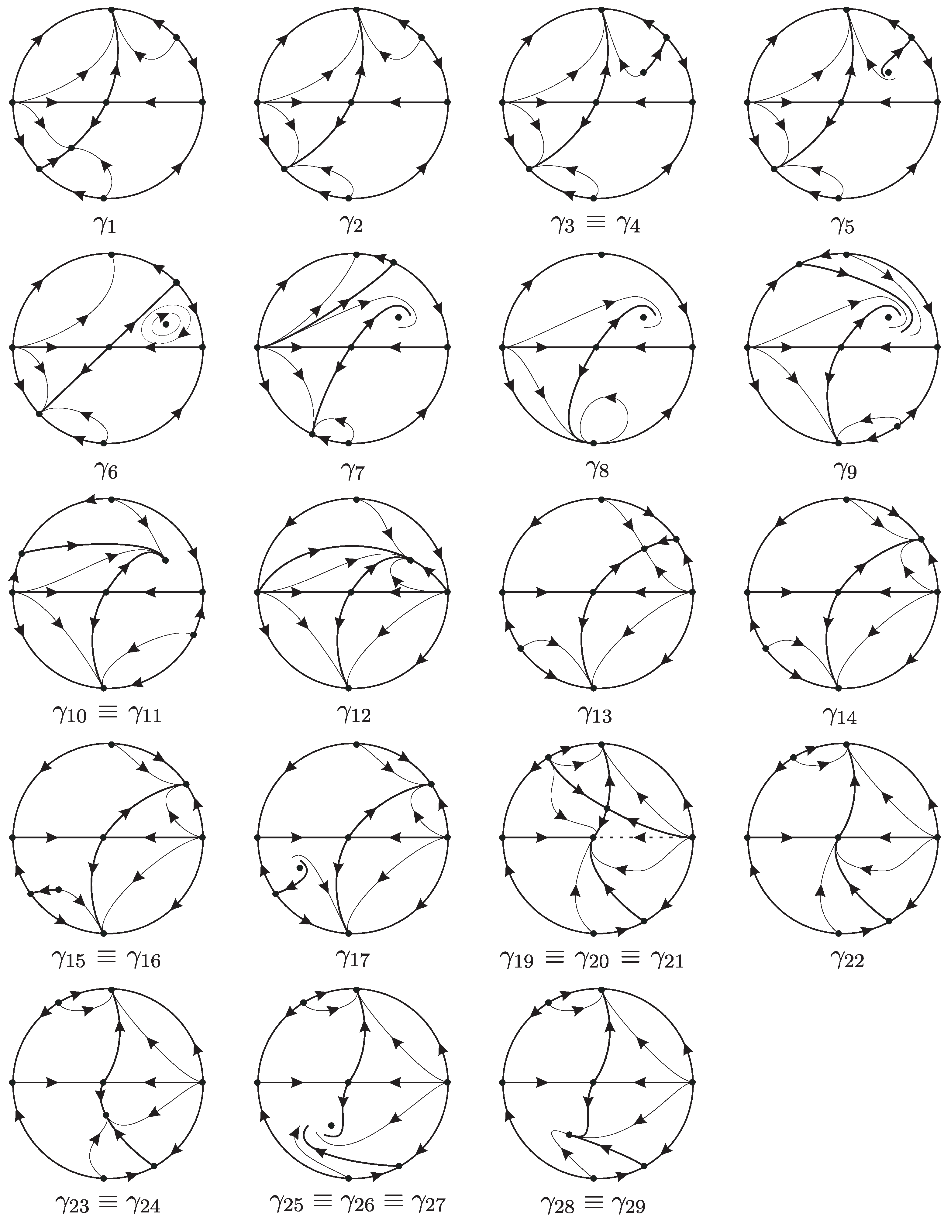
In Figure 1 phase portraits appear which are needed to complete the bifurcation diagram as described in the proof of Theorem 1.

Theorem 2.

The isotropic star having a linear barotropic equation of state modeled by the differential system (1) with $1<\gamma \le 2$ verifies that

(i) 

when $r\to 0$ there is a set of initial conditions of dimension two such that the orbits determined for these conditions satisfy that

$$\frac{m\left(r\right)}{r}\to \infty and4\pi r^2\rho \to 0;$$

(ii) 

There is another set of initial conditions of dimension two such that the orbits determined for these conditions when r tends to some finite value $r_0$ (which depends on the initial conditions) satisfy that

$$\frac{m\left(r\right)}{r}\to 0and4\pi r^2\rho \to k\ge 0,$$

where k can take any positive value when the initial conditions vary;

(iii) 

If

$$\frac{m\left(R\right)}{R}=4\pi R^2\rho =-\frac{2\left({\gamma }^2-2\gamma +1\right)}{{\gamma }^2+4\gamma -4},$$

then

$$\frac{m\left(r\right)}{r}=4\pi r^2\rho =-\frac{2\left({\gamma }^2-2\gamma +1\right)}{{\gamma }^2+4\gamma -4},$$

for all $r\in (0,R]$; finally

(iv) 

There is a set of initial conditions of dimension one such that he orbits determined by these initial conditions when $r\to 0$ satisfy that $m\left(r\right)/r$ and $4\pi r^2\rho$ tend to

$$-\frac{2\left({\gamma }^2-2\gamma +1\right)}{{\gamma }^2+4\gamma -4}.$$

Theorem 2 is proved in Section 3.

2. Proof of Theorem 1

Even the study of the bifurcation diagram of this system is very easy since it has just one parameter, we will make use of the Theory of Invariants developed by the Sibirskii school, and fully developed for quadratic systems in the book [9]. The invariants (and also the comitants) allow us to easily determine all the geometric features provided by the system in a methodic and consistent way. These geometric features may even exceed the most simple topological features to which later we will reduce the classification.

Each one of these geometric features is characterized using some of the following 16 invariant polynomials:

$$\left\{{\mu }_0,{\mu }_1,{\mu }_2,\mathbf{U},W_4,{\mathcal{T}}_3,{\mathcal{T}}_4,{\mathcal{F}}_1,\dots ,{\mathcal{F}}_4,B_1,B_2,B_3,\eta \right\}.$$

(2)

The invariants $B_1$ to $B_3$ can be found in page 14 of [13]. The rest of the invariants can be found on pages 121–128 of [9].

Apart from the geometric properties of the singularities, there may also exist bifurcations due to separatrix connections. If these connections are invariant straight lines or polynomial curves, they may also be determined by means of algebraic invariants. But they may also be of non-algebraic nature in which case, only an analytical and numerical study may detect them. Anyway, we will not meet any of them in this family.

The first important detail to be remarked of this system is that it is not defined for $\gamma =1$. Thus the bifurcation diagram will show a jump from cases with $\gamma <1$ to cases with $\gamma >1$ and no continuity or coherence must be expected from one to the other.

Next, we detect that invariants/comitants ${\mu }_0={\mu }_1$ are equal to zero which proves that two finite singularities have already escaped to infinity, and they will remain there for all the family. Moreover, for every $\gamma$ the straight line $y=0$ is invariant. For some values of $\gamma$ we may have more invariant straight lines. It is a known result that quadratic systems having an invariant straight line can have at most one limit cycle which is either stable or unstable [14], and that quadratic system having two invariant straight lines cannot have limit cycles [15]. Moreover, in this case, the systems have double multiplicity of the line at infinity since we may perturb the first equation by adding a linear factor as $x^{\prime }=(y-x)(1+\epsilon x)$. Since it is known that a quadratic system with two invariant lines cannot have limit cycles, the fact that there exists an invariant line plus a double line at infinity also voids the existence of limit cycles. The reason is that if such a system would have a limit cycle, the mentioned perturbation would produce the second straight line while conserving the limit cycle.

Since we already have ${\mu }_0={\mu }_1=0$, the next relevant comitant is

$${\mu }_2=\frac{\left({\gamma }^2+4\gamma -4\right)y\left(5\gamma x-4x+{\gamma }^{2}y-\gamma y\right)}{{(\gamma -1)}^4}$$

which if it vanishes (for some $\gamma$), will determine if a third singularity escapes to infinity.

We will also need the invariant $\eta =\frac{{\gamma }^2{(5\gamma -4)}^2}{{(\gamma -1)}^6}$ which if equal to zero, determines if two infinite singularities coalesce.

The comitant $\mathbf{U}=\frac{4{(\gamma -2)}^2{y}^2{(x-y)}^2{\left(5\gamma x-4x+{\gamma }^{2}y-\gamma y\right)}^2}{{(\gamma -1)}^6}=0$ tells (in this concrete system) that the two finite singularities coalesce.

And finally, the invariant ${\mathcal{T}}_4=\frac{(\gamma -3)\gamma {(5\gamma -4)}^2\left(3{\gamma }^2-4\right)}{{(\gamma -1)}^8}=0$ tells that one finite singularity is weak (if ${\mathcal{T}}_3\ne 0$), that is, the trace of its Jacobian matrix is zero. This may imply that either it is a weak focus (or a center if more invariants vanish) or it is a weak saddle. There are also invariants to distinguish all these possibilities, and even invariants to determine the level of weakness of the weak point. Anyway, since this system has just one parameter, once ${\mathcal{T}}_4=0$ the system is unique and the weak singularity is fully determined. If ${\mathcal{T}}_4={\mathcal{T}}_3=0$ then either there are two finite weak singularities, or there is a finite nilpotent singularity, or a linearly zero singularity also called intricate singularity in [9], or a singularity with trace zero has escaped to infinity (as it happens for ${\gamma }_8$ and ${\gamma }_{12})$.

Another interesting geometric feature to capture is whether the system has or does not have invariant straight lines. Sometimes these lines will not imply a separatrix connection and thus, breaking them will not produce a different phase portrait. However, at other times, on these lines, we will find separatrix connections and they must be included in the bifurcation diagram. The invariants/comitants that will help us to find those invariant straight lines are $B_1$, $B_2$ and $B_3$. Since $B_1=B_2=0$ for this family, we must just concentrate on $B_3$ which is

$$B_3=-\frac{3(5\gamma -4)\left(3{\gamma }^2-4\right)x^2{y}^2}{{(\gamma -1)}^4}.$$

We normally add one more invariant in every study which is $W_4$. This invariant detects the transition from a node to a strong focus when the invariant changes its sign. This does not produce a topological change in the phase portrait but for the quadratic systems bounds the regions where limit cycles may exist because if a quadratic system has a limit cycle this must surround a focus, see [16]. Since the fact that an antisaddle is a node or a focus may have some physical interest, we have preferred to include it.

In summary, extracting from the different invariant/comitants the equations that must be solved for obtaining the mentioned qualitative information are

$$\begin{array}{cc}\hfill {\gamma }^2+4\gamma -4=& 0,\hfill \\ \hfill \gamma (5\gamma -4)=& 0,\hfill \\ \hfill \gamma -2=& 0,\hfill \\ \hfill (\gamma -3)\gamma (5\gamma -4)(3{\gamma }^2-4)=& 0,\hfill \\ \hfill (5\gamma -4)(3{\gamma }^2-4)=& 0.\hfill \end{array}$$

(3)

Then easy computations determine that the bifurcations points are the values

$$\begin{array}{ccc}{\gamma }_2=-2(1+\sqrt{2}),\hfill & {\gamma }_6=-2\sqrt{3}/3,\hfill & {\gamma }_8=0,\hfill \\ {\gamma }_{12}=4/5,\hfill & {\gamma }_{14}=2(\sqrt{2}-1),\hfill & {\gamma }_{18}=1,\hfill \\ {\gamma }_{20}=2\sqrt{3}/3,\hfill & {\gamma }_{22}=2,\hfill & {\gamma }_{26}=3.\hfill \end{array}$$

(4)

We have enumerated them with even numbers and left some gaps in order to leave space for intermediate generic cases and the values where $W_4=0$. We have also assigned a place for the case $\gamma =1$ even knowing that the differential system is undefined there so as to maintain the coherence in the numeration between generic cases (odd) and singular (even).

The invariant

$$W_4={\gamma }^2{(3\gamma -5)}^2{(5\gamma -4)}^4\left({\gamma }^5-57{\gamma }^4+40{\gamma }^3+408{\gamma }^2-624\gamma +240\right)$$

only changes sign on the roots of the component of degree 5. We must solve it numerically. And now we add intermediate values between each singular values. So to obtain all the bifurcation diagram of this family.

$$\begin{array}{ccc}{\gamma }_1=-5,\hfill & {\gamma }_2=-2(1+\sqrt{2}),\hfill & {\gamma }_3=-4,\hfill \\ {\gamma }_4\approx -2.9649\dots ,\hfill & {\gamma }_5=-2,\hfill & {\gamma }_6=-2\sqrt{3}/3,\hfill \\ {\gamma }_7=-1/2,\hfill & {\gamma }_8=0,\hfill & {\gamma }_9=2/5,\hfill \\ {\gamma }_{10}=\approx 0.76\dots ,\hfill & {\gamma }_{11}=78/100,\hfill & {\gamma }_{12}=4/5,\hfill \\ {\gamma }_{13}=81/100,\hfill & {\gamma }_{14}=2(\sqrt{2}-1),\hfill & {\gamma }_{15}=84/100,\hfill \\ {\gamma }_{16}\approx 0.865822\dots ,\hfill & {\gamma }_{17}=9/10,\hfill & {\gamma }_{18}=1,\hfill \\ {\gamma }_{19}=93/100,\hfill & {\gamma }_{20}=2\sqrt{3}/3,\hfill & {\gamma }_{21}=3/2,\hfill \\ {\gamma }_{22}=2,\hfill & {\gamma }_{23}=21/10,\hfill & {\gamma }_{24}\approx 2.17019\dots ,\hfill \\ {\gamma }_{25}=5/2,\hfill & {\gamma }_{26}=3,\hfill & {\gamma }_{27}=5,\hfill \\ {\gamma }_{28}\approx 56.1619\dots ,\hfill & {\gamma }_{29}=60.\hfill \end{array}$$

(5)

Now using the program P4 (see [12]) we obtain a picture of every phase portrait and we describe briefly the bifurcations, explaining what has happened when we move from one case to another one. In fact, we additionally have verified that all the local phase portraits of the finite and infinite equilibrium points of the differential system (1) are the ones obtained by the program P4. Thus, the local phase portraits of the hyperbolic equilibrium points (i.e., the ones such that the eigenvalues of the linear part of the system evaluated on them have real part non-zero) have been computed with Theorem 2.15 of [12]. The local phase portraits of the semi-hyperbolic or also called semi-elemental equilibrium points (i.e., the ones such that one and only one of the eigenvalues of the linear part of the system evaluated on them is zero) have been computed with Theorem 2.19 of [12]. The local phase portraits of the nilpotent equilibrium points (i.e., the ones such that both eigenvalues of the linear part of the system evaluated on them are zero but the linear part is not identically zero) have been computed with Theorem 3.5 of [12].

We note that when a saddle-node or a nilpotent equilibrium is at infinity the Theorems 2.19 and 3.5 are not sufficient in order to determine the position of the sectors of these points with respect to the line.

Once we know all the local phase portraits of the finite and infinite equilibrium points in order to determine the global phase portraits in the Poincaré disc for the different values of the parameter $\gamma$ we only need to control where start and end the separatrices of the differential system. For the differential systems (1) the separatrices are all the orbits of the infinity, the finite equilibrium points and the separatrices of the hyperbolic sectors of the finite and infinite equilibrium points, for more details see Section 1.9 of [12]. The limit cycles, when they exist, also are separatrices but the differential systems (1) have no separatrices for the reason previously explained.

For ${\gamma }_1$ we see a saddle at the origin and a finite node. The infinite singularity $N_1=[1:0:0]$ is a saddle-node $\overline{\left(\genfrac{}{}{0pt}{}{1}{1}\right)}SN$ (see notation in Section 3.7 or Appendix A of [9]). There is another infinite singularity at $N_2=[0:1:0]$ which is an elemental node, and there is a third equilibrium point at infinity (on the first and third quadrant) $N_3$ which is also a $\overline{\left(\genfrac{}{}{0pt}{}{1}{1}\right)}SN$. The phase portrait is completely determined by the invariant straight line and the distribution of singularities.

For ${\gamma }_2$ we see that the finite node has coalesced with the infinite singularity $N_3$ producing a $\overline{\left(\genfrac{}{}{0pt}{}{2}{1}\right)}N$.

For ${\gamma }_3$ the infinite singularity $N_3$ ejects a node into the first quadrant and becomes again a $\overline{\left(\genfrac{}{}{0pt}{}{1}{1}\right)}SN$.

At ${\gamma }_4$ the node becomes a focus. So the phase portrait is equivalent to the previous one and also to the case ${\gamma }_5$.

At ${\gamma }_6$ the focus becomes weak. But also other invariants, such as ${\mathcal{F}}_1$, ${\mathcal{F}}_2$, and ${\mathcal{F}}_3{\mathcal{F}}_4$ become zero, and thus the singularity is a center. This forces the existence of a separatrix connection between the saddle at the origin and the singularity $N_3$. This connection is required to form the graphic that encloses all the periodic orbits surrounding the center. Moreover, the connection takes place in an invariant straight line. This system is known as $Vulp{e}_{17}$ in the classification [17]. This notation (for quadratic systems with centers) was introduced later in papers like [18].

At ${\gamma }_7$ the center becomes again a focus. Before it was a repellor and now it is an attractor.

At ${\gamma }_8$ the infinite singularity $N_3$ coalesces with $N_2$ producing a nilpotent singularity whose local phase portrait is formed by one elliptic and one hyperbolic sector separated by two parabolic sectors.

For ${\gamma }_9$ the infinite singularity breaks. The singularity $N_3$ is now in the second-fourth quadrant. Somehow, the singularity $N_3$ has transited over $N_1$ and this has required a higher multiplicity singularity.

At ${\gamma }_{10}$ the focus turns back into a node. So the phase portrait is equivalent to the previous one and also to the case ${\gamma }_{11}$.

At ${\gamma }_{12}$ the infinite singularity $N_3$ coalesces with $N_1$ producing an intricate singularity that forces the existence of two parallel invariant straight lines and one hyperbolic sector on each side of infinity. Even though this singularity may seem topologically equivalent (locally) to a semi-elemental saddle-node, it is not because the hyperbolic sectors would have to be in different semiplanes. Moreover, the number of directions arriving at the singularity clearly show their highest codimension.

For ${\gamma }_{13}$ the infinite singularity breaks. The singularity $N_3$ is now again in the third-first quadrant. For ${\gamma }_{14}$ the finite node coalesces again with $N_3$. $N_3$ is again a semi-elemental node of multiplicity 3.

For ${\gamma }_{15}$ the singularity $N_3$ ejects a node into the third quadrant.

At ${\gamma }_{16}$ the node turns back into a focus again. So the phase portrait is equivalent to the previous one and also to the case ${\gamma }_{17}$.

At ${\gamma }_{18}$ we have $\gamma =1$ and the system is undefined. No continuity and no coherence may be expected from what we had before and what we will meet after.

For ${\gamma }_{19}$ we must start describing the phase portrait from zero. We have a node at the origin and a saddle on the upper semiplane. The infinite singularity $N_1$ is a $\overline{\left(\genfrac{}{}{0pt}{}{1}{1}\right)}SN$ as well as $N_3$ which is at the second-fourth quadrant while $N_2$ is a node. We deploy the positive part of halfline $y=0$ with dashes to recall it is an invariant straight line, but it is not a separatrix.

For ${\gamma }_{20}$ we have again a finite weak singularity, but since the origin is a node, it cannot be a weak focus. So the saddle must be weak. Since there is no possibility of the existence of a loop formed by separatrices of this saddle, this produces no topological interest. So, this is equivalent to the previous case and ${\gamma }_{21}$ is also equivalent to ${\gamma }_{19}$.

For ${\gamma }_{22}$ the two finite singularities coalesce forming a semi-elemental saddle-node ${\overline{sn}}_{\left(2\right)}$ (see notation in Section 3.7 or Appendix A of [9]). For ${\gamma }_{23}$ the origin splits, it remains as a saddle and ejects a node into the lower halfplane.

At ${\gamma }_{24}$ the node turns back into a focus. So the phase portrait is equivalent to the previous one and also to the case ${\gamma }_{25}$.

For ${\gamma }_{26}$ we have again a finite weak singularity, and even both focus and saddle have the possibility to be weak, it happens that again the saddle is the weak singularity. Since there is no possibility of the existence of a loop formed by separatrices of this saddle, this produces no topological interest. So, this is equivalent to the previous case and ${\gamma }_{27}$ is also equivalent to ${\gamma }_{25}$.

And at ${\gamma }_{28}$ the focus turns back into a node again. So the phase portrait remains topologically equivalent and also at ${\gamma }_{29}$. Notice also that this phase portrait is topologically equivalent to the case with ${\gamma }_1$.

It must be remarked that this kind of study must normally be conducted in a family of systems whose parameter space may be compactified in a projective space. In this way, one can control also what may happen when one parameter escapes to infinity. Somehow, we may even study the phase portrait when one parameter is ∞. Normally there we find some kind of bifurcation that links both sides (positive and negative of the parameter). Then, by confirming the coherence between the phase portrait at ∞ and the largest (and smallest) $\gamma$ of our bifurcation, we cannot forget any other large singular value of the partition. In general, one cannot affirm that he has found all possible phase portraits, but one can be certain that the whole set is complete and coherent, and that no new slice is needed to obtain the full picture of the diagram. If some other bifurcation occurs, this may not be related to singular points, and whatever occurs, must be undone by another unfound singular slice. This may theoretically occur in a very small part of the parameter space although we have never found such phenomena.

In the current family, it seems that the case $\gamma =\infty$ is not a bifurcation since the phase portrait we obtain for $\gamma >{\gamma }_{23}$ is topologically equivalent to the case $\gamma <{\gamma }_2$. However, we have a problem with the undefined case $\gamma =1$ which will produce a similar phenomena as the described case when $\gamma \to \infty$. That is, we have detected the biggest singular value for $\gamma$ lower than 1 and the lowest greater than 1. But, in general, we cannot know for sure if there are other phantom singular values of $\gamma$ very close to 1.

As this family has a permanent invariant straight line, and there are so few separatrices, it is not hard to see that the phase portrait in every one of the parts that we have divided the straight line, is the corresponding one of Figure 1.

This completes the proof of Theorem 1.

3. Proof of Theorem 2

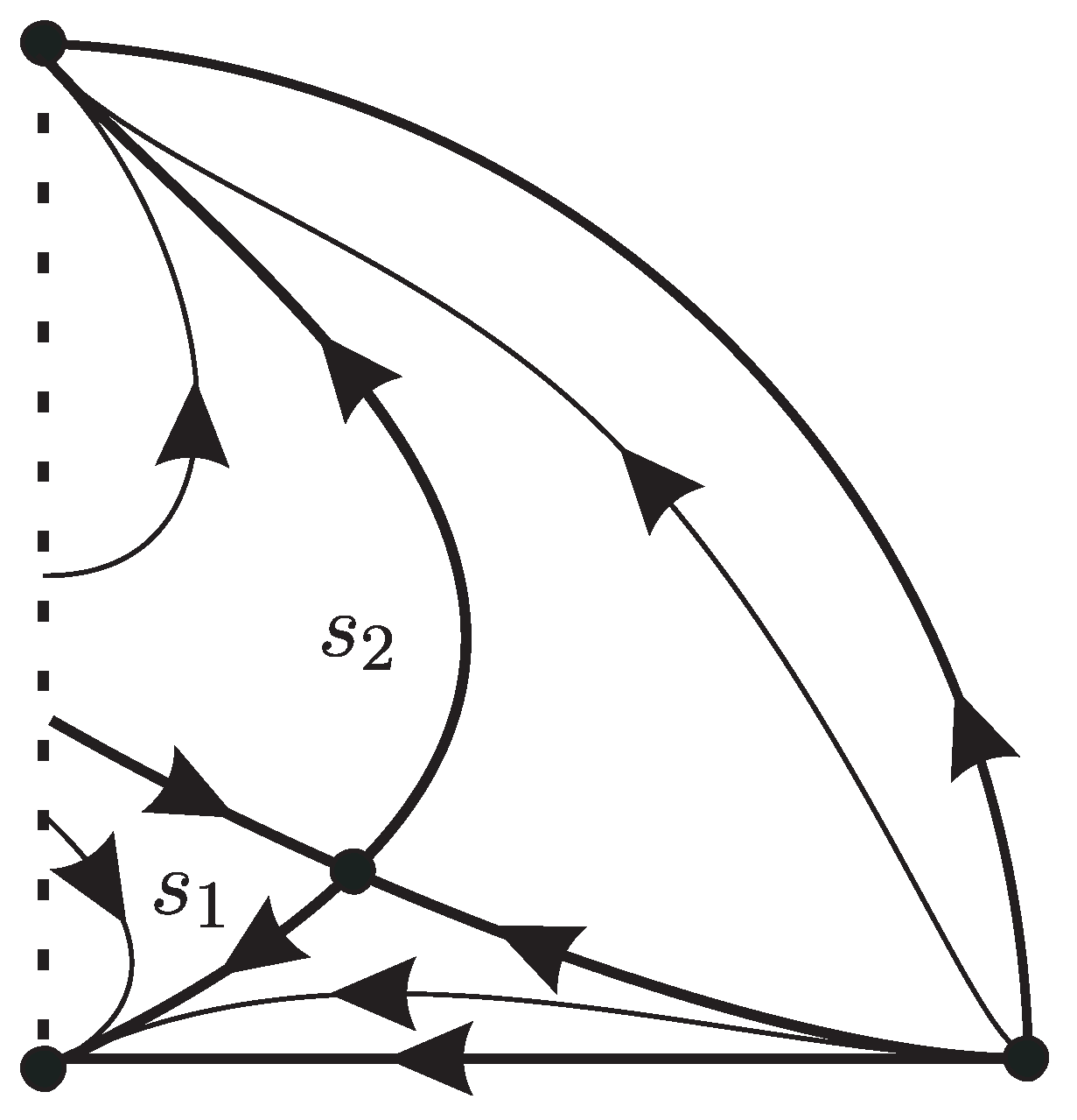
The phase portrait of the differential system (1) when $\gamma \in (1,2]$ is topologically equivalent to the phase portrait ${\gamma }_{19}$. So the restriction of this phase portrait to the positive quadrant Q is shown in Figure 2.

Since $t=ln(r/R)$ and r varies in the interval $(0,R]$, t varies in the interval $(-\infty ,0]$. Taking into account that the meaning of the variables x and y are $x=m\left(r\right)/r>0$ and $y=4\pi r^2\rho >0$, from Figure 2 it follows that all the orbits which are on the right-hand side of the curve formed by the separatrices $s_1$ and $s_2$ of the saddle point

$$P=\left(-\frac{2\left({\gamma }^2-2\gamma +1\right)}{{\gamma }^2+4\gamma -4},-\frac{2\left({\gamma }^2-2\gamma +1\right)}{{\gamma }^2+4\gamma -4}\right),$$

when $r\to 0$ satisfy that

$$\frac{m\left(r\right)}{r}\to \infty \mathrm{and}4\pi r^2\rho \to 0.$$

Hence statement (i) is proved.

While all the orbits are on the left-hand side of the curve formed by the separatrices $s_1$ and $s_2$ of the saddle point P satisfy that

$$\frac{m\left(r\right)}{r}\to 0\mathrm{and}4\pi r^2\rho \to k>0,$$

(6)

for some finite negative value of t, i.e., there is a positive value $r=r_0<R$ for which (6) holds. This completes the proof of statement (ii).

Clearly, the equilibrium point p proves statement (iii).

There are two special orbits, the separatrices $s_1$ and $s_2$ of the saddle P such that when $r\to 0$ they tend to the equilibrium point P. So statement (iv) is proved.

This completes the proof of Theorem 2.

4. Conclusions

In Theorem 1 we have classified all the topologically distinct phase portraits in the Poincaré disc of the family of quadratic systems (1), i.e., of the structure equations of an isotropic star having a linear barotropic equation of state.

In Theorem 2, using the information provided in Theorem 1, if $m\left(r\right)\ge 0$ is the mass inside the sphere of radius r of an isotropic star, and $\rho$ is the density of the isotropic star, we have classified the possible limit values of $m\left(r\right)/r$ and $4\pi r^2\rho$ when r decreases.

References

- Böhmer, C.G.; Harko, T.; Sabau, S.V. Jacobi stability analysis of dynamical systems applications in gravitation and cosmology. Adv. Theor. Math. Phys. 2012, 16, 1145–1196. [Google Scholar] [CrossRef]
- Collins, C.B. Static stars: Some mathematical curiosities. J. Math. Phys. 1977, 18, 1374–1377. [Google Scholar] [CrossRef]
- Khajoei, N. On the dynamic of the isotropic star. Inter. Geom. Meth. Mod. Phys. 2021, 18, 2150165. [Google Scholar] [CrossRef]
- Barraco, D.; Hamity, V.H. Maximum mass of a spherically symmetric isotropic star. Phys. Rev. D 2002, 65, 124028. [Google Scholar] [CrossRef]
- Errehymy, A.; Mustafa, G.; Singh, K.N.; Maurya, S.K.; Daoud, M.; Alrebdi, H.I.; Abdel-Aty, A.H. Electrically charged isotropic stars with Tolman-IV model. New Astron. 2023, 99, 101957. [Google Scholar] [CrossRef]
- Mak, M.K.; Harko, T. Isotropic stars in general relativity. Eur. Phys. J. 2013, 73, 2585. [Google Scholar] [CrossRef]
- Nashed, G.G.L. Isotropic Stars in Higher-Order Torsion Scalar Theories. Adv. High Energy Phys. 2016, 2016, 7020162. [Google Scholar] [CrossRef]
- Pant, N.; Pradhan, N.; Malaver, M. Anisotropic Fluid Star Model in Isotropic Coordinates. Int. Astr. Space Sci. 2015, 3, 1–5. [Google Scholar] [CrossRef]
- Artés, J.C.; Llibre, J.; Schlomiuk, D.; Vulpe, N. Geometric Configurations of Singularities of Planar Polynomial Differential Systems [A Global Classification in the Quadratic Case]; Birkhäuser: Basel, Switzerland, 2021. [Google Scholar]
- Reyn, W. Phase portraits of planar quadratic systems. In Mathematics and Its Applications; Springer: New York, NY, USA, 2007; Volume 583. [Google Scholar]
- Ye, Y. Theory of limit cycles. In Translations of Mathematical Monographs; American Mathematical Society: Providence, RI, USA, 1986; Volume 66. [Google Scholar]
- Dumortier, F.; Llibre, J.; Artés, J.C. Qualitative Theory of Planar Differential Systems; Universitext; Springer: New York, NY, USA; Berlin, Germany, 2006. [Google Scholar]
- Schlomiuk, D.; Vulpe, N. Planar quadratic differential systems with invariant straight lines of at least five total multiplicity. Qual. Theory Dyn. Syst. 2004, 5, 135–194. [Google Scholar] [CrossRef]
- Coll, B.; Llibre, J. Limit cycles for a quadratic system with an invariant straight line and some evolution of phase portraits. In Qualitative Theory of Differential Equations; Colloquia Mathematica Societatis János Bolyai, Bolyai Institut: Szeged, Hungary, 1988; Volume 53, pp. 111–123. [Google Scholar]
- Bautin, N.N. On periodic solutions of a system of differential equations. Differ. Uravn. 1954, 18, 128. [Google Scholar]
- Coppel, W.A. A survey of quadratic systems. J. Differ. Equ. 1966, 2, 293–304. [Google Scholar] [CrossRef]
- Vulpe, N.I. Affine–invariant conditions for the topological distinction of quadratic systems with a center. Differ. Uravn. 1983, 19, 371–379. [Google Scholar]
- Artés, J.C.; Llibre, J.; Schlomiuk, D. The geometry of quadratic differential systems with a weak focus of second order. Int. J. Bifurc. Chaos 2006, 16, 3127–3194. [Google Scholar] [CrossRef]
Figure 1.
Phase portraits of the quadratic systems (1).
Figure 2.
Restriction of system (1) to the first quadrant.
Disclaimer/Publisher’s Note: The statements, opinions and data contained in all publications are solely those of the individual author(s) and contributor(s) and not of MDPI and/or the editor(s). MDPI and/or the editor(s) disclaim responsibility for any injury to people or property resulting from any ideas, methods, instructions or products referred to in the content. |
© 2024 by the authors. Licensee MDPI, Basel, Switzerland. This article is an open access article distributed under the terms and conditions of the Creative Commons Attribution (CC BY) license (https://creativecommons.org/licenses/by/4.0/).
Share and Cite
MDPI and ACS Style
Artés, J.-C.; Llibre, J.; Vulpe, N. Dynamics of the Isotropic Star Differential System from the Mathematical and Physical Point of Views. AppliedMath 2024, 4, 70-78. https://doi.org/10.3390/appliedmath4010004
AMA Style
Artés J-C, Llibre J, Vulpe N. Dynamics of the Isotropic Star Differential System from the Mathematical and Physical Point of Views. AppliedMath. 2024; 4(1):70-78. https://doi.org/10.3390/appliedmath4010004
Chicago/Turabian StyleArtés, Joan-Carles, Jaume Llibre, and Nicolae Vulpe. 2024. "Dynamics of the Isotropic Star Differential System from the Mathematical and Physical Point of Views" AppliedMath 4, no. 1: 70-78. https://doi.org/10.3390/appliedmath4010004