Correlations of ESG Ratings: A Signed Weighted Network Analysis

Abstract

ESG ratings are data-driven indices, focused on three key pillars (Environmental, Social, and Governance), which are used by investors in order to evaluate companies and countries, in terms of Sustainability. A reasonable question which arises is how these ratings are associated to each other. The research purpose of this work is to provide the first analysis of correlation networks, constructed from ESG ratings of selected economies. The networks are constructed based on Pearson correlation and analyzed in terms of some well-known tools from Network Science, namely: degree centrality of the nodes, degree centralization of the network, network density and network balance. We found that the Prevalence of Overweight and Life Expectancy are the most central ESG ratings, while unexpectedly, two of the most commonly used economic indicators, namely the GDP growth and Unemployment, are at the bottom of the list. China’s ESG network has remarkably high positive and high negative centralization, which has strong implications on network’s vulnerability and targeted controllability. Interestingly, if the sign of correlations is omitted, the above result cannot be captured. This is a clear example of why signed network analysis is needed. The most striking result of our analysis is that the ESG networks are extremely balanced, i.e. they are split into two anti-correlated groups of ESG ratings (nodes). It is impressive that USA’s network achieves 97.9% balance, i.e. almost perfect structural split into two anti-correlated groups of nodes. This split of network structure may have strong implications on hedging risk, if we see ESG ratings as underlying assets for portfolio selection. Investing into anti-correlated assets, called as "hedge assets", can be useful to offset potential losses. Our future direction is to apply and extend the proposed signed network analysis to ESG ratings of corporate organizations, aiming to design optimal portfolios with desired balance between risk and return.

1. Introduction

How can we evaluate the performance of a business as “good”? Is it enough to see the profits of the past years? What if the company’s profitable strategy results in depletion of natural resources, pollution of the environment or burden on the local communities in which it operates? If there was a competing business with less profitability, but having a strategy that emphasizes in health, society and the environment, which one would we choose to invest in? In recent years there is a rising global concern about the environment, climate change and sustainability [1]. In this context, investment decisions are increasingly influenced by their environmental impact and sustainability [2]. In the 1990s’ only a few companies published data related to sustainability performance, while in 2020 about 92% of S&P 500 companies and 70% of Russell 1000 companies published such data and reports [3]. ESG indices are used to evaluate the sustainability performance of a company or a country, taking into account Environmental, Social, and Governance concerns [4,5,6,7,8]. In 2006, the UN Principles for Responsible Investment (UNPRI) promoted the integration of ESG criteria into business and investment decisions. By the end of 2021, the adoption of such ESG criteria for investment decisions exceeded 120 trillion dollars of assets under management (AUM) among 3800 signatories of UNPRI [9].

From the investors’ side, the main question is: “Why are ESG data useful and how are utilized for investment decisions?” The motivation of most investors in using ESG data is mainly financial rather than ethical [4]. More specifically, 82% of executives working in investing organizations believe that ESG data are financially important for the performance of investment [4]. This is consistent with meta-analysis studies [5], which show that ESG criteria have positive impact on corporate financial performance. Other important implications of using ESG information in investment decisions is the mitigation of risk [10,11] and portfolio performance [12,13] in times of crisis. Investors who use ESG data usually adopt one of the following three investment strategies [4]: (a) engagement, which is based on the voting power of shareholders, adopting the ESG methodology, in order to influence investment decisions, (b) integration into stock valuation, which includes ESG criteria into financial analysis, and (c) negative screening, which excludes certain assets based on ESG criteria. However the successful integration of ESG information into the investment process has some barriers [4], such as the following: (i) the lack of standards in reporting ESG information, (ii) the lack of comparability across different companies or countries, (iii) the cost of gathering and analyzing the data, (iv) ESG information published by firms are often too general to be useful, and (v) the lack of quantifiable ESG information.

Besides companies and organizations, it is also important for investors to evaluate entire countries with ESG indices. This is mainly because countries with low ESG ratings have less credit worthiness. More specifically, CDS spreads [14,15] and bond yield spreads [16,17] are negatively correlated with ESG ratings. ESG ratings provided by agencies (MSCI, Beyond Ratings, Sustainalytics, etc.) may differ significantly in the case of companies. This is due to different ways of measuring ESG performance; for example, what is the scope of each ESG rating and what are the different components taken into account [18]. On the other hand, in the case of countries, the ESG ratings have no significant differences [19].

ESG ratings are data-driven indices, focused on three key pillars (Environmental, Social, and Governance), which are used by investors in order to evaluate companies and countries, in terms of Sustainability. A reasonable question which arises is how these ratings are associated to each other. Network Theory provides the most well-known mathematical framework for the analysis of interdependencies [20]. Networks consist of nodes $\mathsf{\kappa }=1,2,\dots ,N$ connected via links. In our work, the nodes represent the ESG indices, while the links are weighted according to the Pearson correlation coefficient. As a result, each link $\left(\mathsf{\kappa },\lambda \right)$ is characterized by the corresponding weight $w_{\mathsf{\kappa }\lambda }$, describing the sign and the strength of relationship between the two nodes $\mathsf{\kappa }$ and $\lambda$. In this way, we construct networks from the correlations between the ESG indices. The aim of our work is to analyze these networks using some well-known tools from Network Science, namely, the following: degree centrality of the nodes, degree centralization of the network, network density and network balance. Degree centrality measures the extent to which a node is connected–correlated with other nodes. Therefore, degree centrality gives us information about how “central” a node is within the network, based on its connections–correlations with other nodes. While degree centrality is a local index, referring to nodes, degree centralization is a global index, referring to the network as a whole. More specifically, if there are a few “central” nodes in the network, then the network is considered as “centralized” and, therefore, the degree centralization is high. In this case, where the degree centralization of the network is high, the dynamics of each node is highly interdependent on the dynamics of the few central nodes, called “hubs”. Network density is also a global index, which is defined as the ratio of the existing link weights to the maximum possible link weights that may occur. In other words, density measures how dense the link weights are within the network, expressing how much the different nodes/variables are interdependent. For example, if a correlation network is sparse, this means that the nodes/variables are not highly interdependent. In other words, the dynamics of each node is weakly correlated with the dynamics of the other nodes of the network. Network balance is also a global index, originally defined for social networks, which measures the extent to which a network can be separated into two groups of nodes, where intra-group weights are positive, and inter-group weights are negative. Further clarification of the above tools, as well as their formal mathematical definitions and relevant references, are provided in Section 2, Materials and Methods.

It is said that, if Sustainable Development Indicators influence each other, then the actions which are made to improve one specific indicator, may cause “synergies” (co-benefits) or “impairments” (trade-offs) to others [21,22]. In the same line of thinking, the rise or fall of some highly correlated ESG indices may trigger strong fluctuations in the rest of the ESG ratings. This instability is translated into uncertainty for ESG-based investors. Therefore, the study of correlations between ESG ratings with Network Theory is of high importance, because, in this way, the most central, highly correlated, ESG ratings (nodes), as well as the groups of similarly correlated or anti-correlated nodes, are clearly captured. It is worth mentioning that this is the first analysis of correlation networks from ESG ratings. Therefore, the contribution of our work to professionals and academics results from providing the first insight into the structure of ESG interdependencies. More specifically, we found that the Prevalence of Overweight and Life Expectancy are the most central ESG ratings, while, unexpectedly, two of the most commonly used economic indicators, namely GDP growth and Unemployment, are at the bottom of the list. Furthermore, China’s ESG network has remarkably high positive and high negative centralization, implying that there are only a few central, highly correlated, ESG indices. The most striking result of our analysis was the finding that the ESG networks are extremely balanced, i.e., they can be split into two anti-correlated groups of ESG ratings (nodes). Specifically, for the USA, the ESG correlation network achieved 97.9% balance, i.e., almost perfect structural split into two anti-correlated groups of nodes. This split of network structure may have strong implications on hedging risk, if we see ESG ratings as underlying assets for portfolio selection. This is because, investing in anti-correlated assets, called “hedge assets”, can be useful to offset potential losses. The results of our work are presented in detail in Section 3, Results and Discussion.

Network analysis of correlations is a well-established methodology, which has been applied widely to several topics. For example, in financial networks, the analysis of the relevant networks is useful for the study of risk contagion in financial markets [23,24,25,26,27,28], while in brain networks, the relevant correlation networks have been analyzed as signed graphs [29]. Recently, network analysis has been applied to the relationships between the Sustainable Development Indicators. The United Nations adopted, in 2015, a plan of 17 Sustainable Development Goals (SDGs) and 169 associated targets, aiming to eradicate poverty, protect the planet and ensure peace and well-being for all people by 2030 [30]. Of course, these goals are not independent. On the contrary, they influence each other, in the sense that actions taken to improve one specific indicator, may cause “synergies” (co-benefits) or “impairments” (trade-offs) to others [21,22]. For the analysis of the interdependencies between the 17 SDGs, both qualitative and quantitative approaches have been proposed. Concerning qualitative approaches, the International Council for Science, published in 2015, was the first analysis of interconnections between the SDGs and their associated targets [31]. After the work of Nilsson et al. [32], where a seven-point scale (from −3 to +3) was introduced to assess the links between the goals, another important analysis was published [33], where the authors specified the dependencies between the SDGs and their associated targets, taking into account the seven-point scale of Nilsson et al. Many papers rely on such qualitative estimations of the links, in order to construct relations networks of the SDGs and their associated targets [22,34,35,36].

In addition to the aforementioned qualitative approach in analyzing the relationships between Sustainable Development Indicators, there are also quantitative studies which analyze correlation networks, constructed from Sustainable Development Indicators. More specifically, these correlation networks are usually based on Pearson or Spearman correlation coefficient, and, therefore, they have both positive and negative link weights. As a result, they are treated as signed networks [21,37,38,39,40,41,42]. Furthermore, causal networks of Sustainable Development Indicators have also been constructed, based on Granger Causality [43]. In this case, the networks are treated as directed graphs. The usual network analysis includes node centralities, aiming to rank the importance of nodes (Sustainable Development Indicators) in terms of their connectivity [21,37,40,41,44].

Our work provides the first quantitative network analysis of correlations between ESG ratings, as estimated from the Pearson correlation coefficient, with data provided by the World Bank. The constructed correlation networks are treated as signed weighted graphs. Therefore, the usual network analysis (degree centralities of the nodes, degree centralization of the network, network density) has been extended in order to be applicable to signed weighted graphs. In addition to the above tools, we analyze the ESG correlation networks in terms of Network Balance, which measures the extent to which there are antagonistic (anti-correlated) groups of nodes in the network. The existence of antagonistic groups of nodes was mentioned for networks constructed from sustainable development indicators [21]. In the same line of thinking, we explore the existence of such “network split” quantitatively, in networks constructed from ESG ratings.

The rest of the paper is structured as follows. In Section 2, we specify the economies and the ESG indices to be studied, the relevant data, as well as how the networks are constructed and assessed. In Section 3, we present the results from network analysis. In Section 4, we summarize the concluding remarks and the impact of our findings.

2. Materials and Methods

We used the ESG dataset of the World Bank [45], which provides data on an annual basis. We studied 25 ESG indices for 16 economies over a time period from 1990 to 2015, due to data availability. The 16 economies are the following: (a) 13 countries (China, the United Kingdom, the United States, Japan, Germany, Austria, Denmark, Finland, France, Greece, the Netherlands, Norway, Sweden), (b) two economic associations (OECD, Euro Area), and (c) High-Income Countries. The 25 ESG indices are categorized as follows: (i) 13 are related to environmental concerns (Agricultural land, CO₂ emissions, Electricity production from coal sources, Energy imports, Energy use, Food production, Forest area, Fossil fuel energy consumption, Methane emissions, Nitrous oxide emissions, Population density, Renewable electricity output, Renewable energy consumption), (ii) 8 are related to social concerns (Fertility rate, Hospital beds, Life expectancy, Mortality rate under-5, Population ages 65 and above, Prevalence of overweight, Labor force participation rate, Unemployment), and (iii) 4 governance concerns (GDP growth, Patent applications, Ratio of female to male labor force participation rate, Individuals using the Internet). We studied the resulting correlation networks, where the nodes $\mathsf{\kappa }=1,2,\dots ,\mathrm{N}$ represent the 25 ESG indices and the links are undirected and signed weighted according to the Pearson correlation coefficient defined below.

Definition 1. 

Pearson Correlation Matrix $C=\left(c_{\mathsf{\kappa }\lambda }\right)$.

The Pearson Correlation Coefficient ${\mathrm{c}}_{\mathsf{\kappa }\mathsf{\lambda }}$ estimates the linear correlation between two variables, namely $\mathsf{\kappa }$ and $\mathsf{\lambda }$, as follows:

$${\mathrm{c}}_{\mathsf{\kappa }\mathsf{\lambda }}=\frac{{{\displaystyle \sum }}_{\mathrm{t}=1990}^{2015}\left[\left({\mathrm{x}}_{\mathsf{\kappa }}\left(\mathrm{t}\right)-{\mathrm{m}}_{\mathsf{\kappa }}\right)·\left({\mathrm{x}}_{\mathsf{\lambda }}\left(\mathrm{t}\right)-{\mathrm{m}}_{\mathsf{\lambda }}\right)\right]}{\sqrt{{{\displaystyle \sum }}_{\mathrm{t}=1990}^{2015}{\left({\mathrm{x}}_{\mathsf{\kappa }}\left(\mathrm{t}\right)-{\mathrm{m}}_{\mathsf{\kappa }}\right)}^2}·\sqrt{{{\displaystyle \sum }}_{\mathrm{t}=1990}^{2015}{\left({\mathrm{x}}_{\mathsf{\lambda }}\left(\mathrm{t}\right)-{\mathrm{m}}_{\mathsf{\lambda }}\right)}^2}}$$

where ${\mathrm{x}}_{\mathsf{\kappa }}\left(\mathrm{t}\right)$ and ${\mathrm{x}}_{\mathsf{\lambda }}\left(\mathrm{t}\right)$ are the observations of the two variables-ESG indices (nodes) $\mathsf{\kappa }$ and $\mathsf{\lambda }$ correspondingly, while ${\mathrm{m}}_{\mathsf{\kappa }}$ and ${\mathrm{m}}_{\mathsf{\lambda }}$ are the corresponding mean values of observations. The resulting Correlation Matrix $\mathrm{C}=\left({\mathrm{c}}_{\mathsf{\kappa }\mathsf{\lambda }}\right)$ below is a square N × N = 25 × 25 matrix with elements taking values $-1\le {\mathrm{c}}_{\mathsf{\kappa }\mathsf{\lambda }}\le 1$:

$$\mathrm{C}=\left({\mathrm{c}}_{\mathsf{\kappa }\mathsf{\lambda }}\right)=\left(\begin{array}{ccccc}{\mathrm{c}}_{11}& {\mathrm{c}}_{12}& {\mathrm{c}}_{13}& \cdots & {\mathrm{c}}_{1\mathrm{N}}\\ {\mathrm{c}}_{21}& {\mathrm{c}}_{22}& {\mathrm{c}}_{23}& \cdots & {\mathrm{c}}_{2\mathrm{N}}\\ {\mathrm{c}}_{31}& {\mathrm{c}}_{32}& {\mathrm{c}}_{33}& \cdots & {\mathrm{c}}_{3\mathrm{N}}\\ ⋮& ⋮& ⋮& ⋮& ⋮\\ {\mathrm{c}}_{\mathrm{N}1}& {\mathrm{c}}_{\mathrm{N}2}& {\mathrm{c}}_{\mathrm{N}3}& \cdots & {\mathrm{c}}_{\mathrm{NN}}\end{array}\right)=\left(\begin{array}{ccccc}1& {\mathrm{c}}_{12}& {\mathrm{c}}_{13}& \cdots & {\mathrm{c}}_{1\mathrm{N}}\\ {\mathrm{c}}_{21}& 1& {\mathrm{c}}_{23}& \cdots & {\mathrm{c}}_{2\mathrm{N}}\\ {\mathrm{c}}_{31}& {\mathrm{c}}_{32}& 1& \cdots & {\mathrm{c}}_{3\mathrm{N}}\\ ⋮& ⋮& ⋮& ⋮& ⋮\\ {\mathrm{c}}_{\mathrm{N}1}& {\mathrm{c}}_{\mathrm{N}2}& {\mathrm{c}}_{\mathrm{N}3}& \cdots & 1\end{array}\right)$$

Definition 2. 

Weight Matrix $W=\left(w_{\mathsf{\kappa }\lambda }\right)$.

The Weight Matrix $\mathrm{W}=\left({\mathrm{w}}_{\mathsf{\kappa }\mathsf{\lambda }}\right)$ is constructed from the correlation matrix $\mathrm{C}$ as follows. First, we eliminate the diagonal elements of the correlation matrix representing autocorrelations. Second, we eliminate the off-diagonal elements of the correlation matrix with weak correlations, namely ${ \mathrm{c}}_{\mathsf{\kappa }\mathsf{\lambda }}\in \left[-0.1,+0.1\right]$. This “threshold method” is standard in correlation network analysis [27] in order to reduce the complexity and facilitate the analysis and retain the most significant relationships. We tried different small thresholds and we selected 10%, because, in this case, the weights variations were visualized more clearly and the results were captured more easily. The weight matrix $\mathrm{W}$ has the following form:

$$\mathrm{W}=\left({\mathrm{w}}_{\mathsf{\kappa }\mathsf{\lambda }}\right)=\left(\begin{array}{ccccc}0& {\mathrm{w}}_{12}& {\mathrm{w}}_{13}& \cdots & {\mathrm{w}}_{1\mathrm{N}}\\ {\mathrm{w}}_{21}& 0& {\mathrm{w}}_{23}& \cdots & {\mathrm{w}}_{2\mathrm{N}}\\ {\mathrm{w}}_{31}& {\mathrm{w}}_{32}& 0& \cdots & {\mathrm{w}}_{3\mathrm{N}}\\ ⋮& ⋮& ⋮& ⋮& ⋮\\ {\mathrm{w}}_{\mathrm{N}1}& {\mathrm{w}}_{\mathrm{N}2}& {\mathrm{w}}_{\mathrm{N}3}& \cdots & 0\end{array}\right)$$

where ${\mathrm{w}}_{\mathsf{\kappa }\mathsf{\lambda }}=⟦{ \mathrm{c}}_{\mathsf{\kappa }\mathsf{\lambda }}\notin \left[-0.1,+0.1\right]⟧·{\mathrm{c}}_{\mathsf{\kappa }\mathsf{\lambda }}$.

The term $⟦\mathrm{Q}⟧$ is the Iverson bracket [46] which converts Boolean values to numbers $0, 1$:

$$⟦\mathrm{Q}⟧ =\left\{\begin{array}{c}1, \mathrm{if} \mathrm{Q} \mathrm{is} \mathrm{True}\\ 0, \mathrm{if} \mathrm{Q} \mathrm{is} \mathrm{False}\end{array}\right.$$

The network, corresponding to weight matrix $\mathrm{W}$, is signed weighted undirected with no self-loops. From weight matrix $\mathrm{W}$ we can define the following relevant matrices.

Definition 3. 

Absolute Weight Matrix $\left|W\right|=\left(\left|w_{\mathsf{\kappa }\lambda }\right|\right)$.

The Absolute Weight Matrix $\left|\mathrm{W}\right|=\left(\left|{\mathrm{w}}_{\mathsf{\kappa }\mathsf{\lambda }}\right|\right)$ is simply the absolute value of weight matrix $\mathrm{W}$. The corresponding network is positively weighted undirected with no self-loops.

Definition 4. 

Positive$W^{+}=\left(w_{\mathsf{\kappa }\lambda }^{+}\right)$and Negative$W^{-}=\left(w_{\mathsf{\kappa }\lambda }^{-}\right)$Weight Matrices.

The Positive Weight Matrix ${\mathrm{W}}^{+}=\left({\mathrm{w}}_{\mathsf{\kappa }\mathsf{\lambda }}^{+}\right)$ has the non-negative elements of weight matrix $\mathrm{W}$, while the Negative Weight Matrix ${\mathrm{W}}^{-}=\left({\mathrm{w}}_{\mathsf{\kappa }\mathsf{\lambda }}^{-}\right)$ has the non-positive elements of weight matrix $\mathrm{W}$. The elements of ${\mathrm{W}}^{+}$ and ${\mathrm{W}}^{-}$ are defined correspondingly as: ${\mathrm{w}}_{\mathsf{\kappa }\mathsf{\lambda }}^{+}=⟦{\mathrm{w}}_{\mathsf{\kappa }\mathsf{\lambda }}>0⟧·{\mathrm{w}}_{\mathsf{\kappa }\mathsf{\lambda }}$ and ${\mathrm{w}}_{\mathsf{\kappa }\mathsf{\lambda }}^{-}=⟦{\mathrm{w}}_{\mathsf{\kappa }\mathsf{\lambda }}<0⟧·{\mathrm{w}}_{\mathsf{\kappa }\mathsf{\lambda }}$, where the term $⟦\mathrm{Q}⟧$ is the Iverson bracket [46] defined above. The two corresponding networks are weighted (positively for ${\mathrm{W}}^{+}$ and negatively for ${\mathrm{W}}^{-}$) undirected with no self-loops.

We define below some useful metrics from Network Theory for assessing individual nodes (local metrics), as well as for assessing the network as a whole (global metrics). We also briefly present the concept of Balance for signed undirected networks.

Definition 5. 

Degree (Local Metric).

The Degree ${\mathrm{deg}}_{\mathsf{\kappa }}$ of node $\mathsf{\kappa }$ is defined [29] as the sum of links with all its first distinct neighbours, taking values within the interval $\left[0,\mathrm{N}-1\right]$. Degree measures the extent to which a node is connected-correlated with other nodes. Therefore, degree gives us information about how “central” is a node within the network, based on its connections–correlations with other nodes. For weight matrices $\left|\mathrm{W}\right|, {\mathrm{W}}^{+}, {\mathrm{W}}^{-}$, we define in

Table 1. Degree${\mathrm{deg}}_{\mathsf{\kappa }}$ of node $\mathsf{\kappa }$.

Matrix	Name	Formula
$\left|\mathrm{W}\right|$	Absolute weighted degree	${\mathrm{deg}}_{\mathsf{\kappa }}^{\left|\mathrm{w}\right|}={\displaystyle {\displaystyle \sum }_{\begin{array}{c}\mathsf{\nu }=1\\ \mathsf{\nu }\ne \mathsf{\kappa }\end{array}}^{\mathsf{{\rm N}}}}\left|{\mathrm{w}}_{\mathsf{\kappa }\mathsf{\nu }}\right|$
${\mathrm{W}}^{+}$	Positive weighted degree	${\mathrm{deg}}_{\mathsf{\kappa }}^{\left[\mathrm{w}\right]+}={\displaystyle {\displaystyle \sum }_{\begin{array}{c}\mathsf{\nu }=1\\ \mathsf{\nu }\ne \mathsf{\kappa }\end{array}}^{\mathsf{{\rm N}}}}{\mathrm{w}}_{\mathsf{\kappa }\mathsf{\nu }}^{+}$
${\mathrm{W}}^{-}$	Negative weighted degree	${\mathrm{deg}}_{\mathsf{\kappa }}^{\left[\mathrm{w}\right]-}={\displaystyle {\displaystyle \sum }_{\begin{array}{c}\mathsf{\nu }=1\\ \mathsf{\nu }\ne \mathsf{\kappa }\end{array}}^{\mathsf{{\rm N}}}}\left|{\mathrm{w}}_{\mathsf{\kappa }\mathsf{\nu }}^{-}\right|$

the corresponding weighted degrees of node $\mathsf{\kappa }$, which also take values within the interval $\left[0,\mathrm{N}-1\right]$.

Definition 6. 

Degree Centrality (Local Metric).

The Degree Centrality ${\mathrm{DEG}}_{\mathsf{\kappa }}$ of node $\mathsf{\kappa }$ is defined [47] as the normalized degree ${\mathrm{deg}}_{\mathsf{\kappa }}$, taking values within the interval $\left[0,1\right]$. For weight matrices $\left|\mathrm{W}\right|, {\mathrm{W}}^{+}, {\mathrm{W}}^{-}$, we define in

Table 2. Degree Centrality ${\mathrm{DEG}}_{\mathsf{\kappa }}$ of node $\mathsf{\kappa }$.

Matrix	Name	Formula
$\left|\mathrm{W}\right|$	Absolute weighted degree centrality	${\mathrm{DEG}}_{\mathsf{\kappa }}^{\left|\mathrm{w}\right|}=\frac{{\mathrm{deg}}_{\mathsf{\kappa }}^{\left|\mathrm{w}\right|}}{\mathrm{N}-1}$
${\mathrm{W}}^{+}$	Positive weighted degree centrality	${\mathrm{DEG}}_{\mathsf{\kappa }}^{\left[\mathrm{w}\right]+}=\frac{{\mathrm{deg}}_{\mathsf{\kappa }}^{\left[\mathrm{w}\right]+}}{\mathrm{N}-1}$
${\mathrm{W}}^{-}$	Negative weighted degree centrality	${\mathrm{DEG}}_{\mathsf{\kappa }}^{\left[\mathrm{w}\right]-}=\frac{{\mathrm{deg}}_{\mathsf{\kappa }}^{\left[\mathrm{w}\right]-}}{\mathrm{N}-1}$

the corresponding weighted degrees centralities of node $\mathsf{\kappa }$, which also take values within the interval $\left[0,1\right]$.

Definition 7. 

Degree Centralization (Global Metric).

The Degree Centralization of a network is a key metric with values in the interval $\left[0,1\right]$, which measures how central the most central node $\mathsf{\xi }$ is, in relation to how central all the other nodes $\mathsf{\kappa }=1,2,\dots ,\mathrm{N}$ are [47]. While degree centrality is a local index referring to nodes, degree centralization is a global index referring to the network as a whole. More specifically, if there are a few “central” nodes in the network, then the network is considered as “centralized” and, therefore, the degree centralization is high. The degree centralization $\mathrm{DEG}$ of a network is defined [47] by the following fraction:

$$\mathrm{DEG}=\frac{{{\displaystyle \sum }}_{\mathsf{\kappa }=1}^{\mathsf{{\rm N}}}\left({\mathrm{DEG}}_{\mathsf{\xi }}-{\mathrm{DEG}}_{\mathsf{\kappa }}\right)}{\mathrm{N}-2}$$

where:${ \mathrm{DEG}}_{\mathsf{\xi }}=\underset{\mathsf{\kappa }=1,2,\dots ,\mathsf{{\rm N}}}{\max }\left\{{\mathrm{DEG}}_{\mathsf{\kappa }}\right\}$

The numerator is the sum of differences between the degree centralities of the most central node $\mathsf{\xi }$ and all other nodes $\mathsf{\kappa }=1,2,\dots ,\mathrm{N}$. The denominator is the theoretically largest sum of such differences in any network of the same size. The theoretically largest sum of such differences is achieved for the undirected “star” network topology. This network topology consists of one “star” (central) node $\mathsf{\xi }$ which has links with all other “satellite” nodes (with maximal possible weight equal to one), and “satellite” nodes have no links with other “satellite” nodes. In other words, for the undirected “star” network topology, we have:${\mathrm{DEG}}_{\mathsf{\xi }}=\frac{\mathrm{N}-1}{\mathrm{N}-1}=1$ and ${\mathrm{DEG}}_{\mathsf{\kappa }}=\frac{1}{\mathrm{N}-1}$ for $\mathsf{\kappa }=1,2,\dots ,\mathsf{{\rm N}}$ with $\mathsf{\kappa }\ne \mathsf{\xi }$.

For weight matrices $\left|\mathrm{W}\right|, {\mathrm{W}}^{+}, {\mathrm{W}}^{-}$, we define in

Table 3. Degree Centralization $\mathrm{DEG}$ of the network.

Matrix	Name	Formula
$\left|\mathrm{W}\right|$	Absolute weighted degree centralization	${\mathrm{DEG}}^{\left|\mathrm{w}\right|}=\frac{{{\displaystyle \sum }}_{\mathsf{\kappa }=1}^{\mathsf{{\rm N}}}\left({\mathrm{DEG}}_{\mathsf{\xi }}^{\left|\mathrm{w}\right|}- {\mathrm{DEG}}_{\mathsf{\kappa }}^{\left|\mathrm{w}\right|}\right)}{\mathrm{N}-2}$
${\mathrm{W}}^{+}$	Positive weighted degree centralization	${\mathrm{DEG}}^{\left[\mathrm{w}\right]+}=\frac{{{\displaystyle \sum }}_{\mathsf{\kappa }=1}^{\mathsf{{\rm N}}}\left({\mathrm{DEG}}_{\mathsf{\xi }}^{\left[\mathrm{w}\right]+}- {\mathrm{DEG}}_{\mathsf{\kappa }}^{\left[\mathrm{w}\right]+}\right)}{\mathrm{N}-2}$
${\mathrm{W}}^{-}$	Negative weighted degree centralization	${\mathrm{DEG}}^{\left[\mathrm{w}\right]-}=\frac{{{\displaystyle \sum }}_{\mathsf{\kappa }=1}^{\mathsf{{\rm N}}}\left({\mathrm{DEG}}_{\mathsf{\xi }}^{\left[\mathrm{w}\right]-}- {\mathrm{DEG}}_{\mathsf{\kappa }}^{\left[\mathrm{w}\right]-}\right)}{\mathrm{N}-2}$

the corresponding weighted degrees centralizations of the networks, which also take values within the interval $\left[0,1\right]$.

Definition 8. 

Network Density (Global Metric).

The Density of a network is also a key metric with values in the interval [0,1], which measures how dense the link weights within the network are [47]. The density expresses how much the different nodes/variables are interdependent. For example, if a correlation network is sparse, this means that the nodes/variables are not highly interdependent. In other words, the dynamics of each node is weakly correlated with the dynamics of the other nodes of the network. The density $\mathrm{DEN}$ of a network is defined [47] as a fraction where the numerator is the sum of existing off-diagonal link weights and the denominator is the sum of maximal possible off-diagonal link weights. In other words, the denominator corresponds to a theoretical complete network of the same size, where all off-diagonal links are present (with maximal possible weight equal to one). For weight matrices $\left|\mathrm{W}\right|, {\mathrm{W}}^{+}, {\mathrm{W}}^{-}$, we define in

Table 4. Network Density $\mathrm{DEN}$.

Matrix	Name	Formula
$\left|\mathrm{W}\right|$	Absolute weighted density	${\mathrm{DEN}}^{\left|\mathrm{w}\right|}=\frac{{{\displaystyle \sum }}_{\mathsf{\kappa }=1}^{\mathsf{{\rm N}}}\left({{\displaystyle \sum }}_{\begin{array}{c}\mathsf{\nu }=1\\ \mathsf{\nu }\ne \mathsf{\kappa }\end{array}}^{\mathsf{{\rm N}}}\left|{\mathrm{w}}_{\mathsf{\kappa }\mathsf{\nu }}\right|\right)}{\mathrm{N}·\left(\mathrm{N}-1\right)}$
${\mathrm{W}}^{+}$	Positive weighted density	${\mathrm{DEN}}^{\left[\mathrm{w}\right]+}=\frac{{{\displaystyle \sum }}_{\mathsf{\kappa }=1}^{\mathsf{{\rm N}}}\left({{\displaystyle \sum }}_{\begin{array}{c}\mathsf{\nu }=1\\ \mathsf{\nu }\ne \mathsf{\kappa }\end{array}}^{\mathsf{{\rm N}}}{\mathrm{w}}_{\mathsf{\kappa }\mathsf{\nu }}^{+}\right)}{\mathrm{N}·\left(\mathrm{N}-1\right)}$
${\mathrm{W}}^{-}$	Negative weighted density	${\mathrm{DEN}}^{\left[\mathrm{w}\right]-}=\frac{{{\displaystyle \sum }}_{\mathsf{\kappa }=1}^{\mathsf{{\rm N}}}\left({{\displaystyle \sum }}_{\begin{array}{c}\mathsf{\nu }=1\\ \mathsf{\nu }\ne \mathsf{\kappa }\end{array}}^{\mathsf{{\rm N}}}\left|{\mathrm{w}}_{\mathsf{\kappa }\mathsf{\nu }}^{-}\right|\right)}{\mathrm{N}·\left(\mathrm{N}-1\right)}$

the corresponding weighted densities of the networks, which also take values within the interval $\left[0,1\right]$.

As weight matrix $\mathrm{W}$ corresponds to a signed undirected network, it is interesting to examine to what extent this network is balanced. We briefly present the concept of Balance for signed undirected networks. Structural Balance Theory, proposed by Heider, was based on triangles [48,49] within the context of social relationships and attitude change. Harary and Cartwright formulated Heider’s theory mathematically, using signed undirected networks [50,51]. A triangle is considered as “balanced” if the multiplication of the signs of the links is positive. As a result, a balanced triangle may consist of either three positive links or two negative links with one positive link. Otherwise, the triangle is unbalanced. The simplest way to measure network balance is to compute the fraction of balanced triangles [51]. However, this way may not give a satisfactory measure of the global balance of the network, i.e., a network may not be globally balanced, although all triangles are balanced [52].

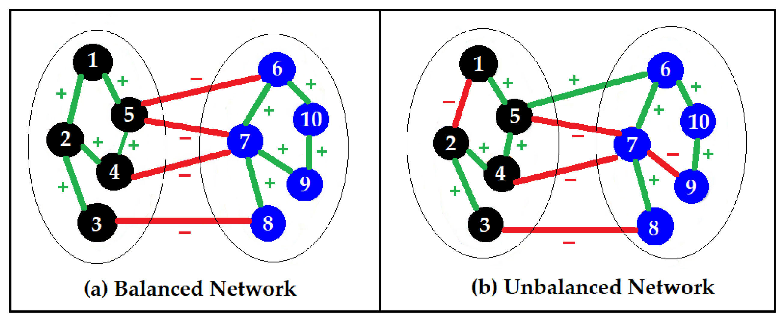
In this paper, we are interested in measuring network balance based on frustration. That is because frustration-based balance measures how close the network is to a structural split of two groups, where intra-group weights are positive and inter-group weights are negative (Figure 1). Each node has one of two possible colors, for example, either black or blue, as illustrated in Figure 1. Frustrated links are defined as the links that are either negative intra-group (links 1–2 and 7–9 in Figure 1b) or positive inter-group (link 5–6 in Figure 1b). In this way, Frustration $\mathrm{F}$ is defined as the smallest number of frustrated links over all possible 2-colorings of the nodes (black–blue) of a network.

Definition 9. 

Network Balance (Global Metric).

The Balance of a network is defined based on Frustration $\mathrm{F}$, taking values from 0 (perfect unbalance) to 1 (perfect balance) as follows:

$${\mathrm{BAL}}^{\left[\mathrm{w}\right]}=1-\frac{\mathrm{F}}{{{\displaystyle \sum }}_{\mathsf{\kappa }=1}^{\mathsf{{\rm N}}}\left({{\displaystyle \sum }}_{\begin{array}{c}\mathsf{\nu }=1\\ \mathsf{\nu }\ne \mathsf{\kappa }\end{array}}^{\mathsf{{\rm N}}}⟦{\mathrm{w}}_{\mathsf{\kappa }\mathsf{\nu }}\ne 0⟧\right)}$$

For more details on measuring network balance based on frustration, we refer to the work of Aref [53]. The calculations were implemented computationally using the relevant “signet” package [54] in R programming language.

3. Results and Discussion

In this section we present and discuss the results of our analysis. More specifically, in Section 3.1 we present the results for individual nodes, the ESG indices (local analysis), based on degree centrality and egonets. In Section 3.2 we present the results for each network, the economy as a whole (global analysis), based on degree centralization, network density, and network balance. We make specific remarks in order to highlight notable results. For data analysis and visualization, we used the R programming language and relevant packages available on CRAN [55].

3.1. Local Analysis (Degree Centrality, Egonets)

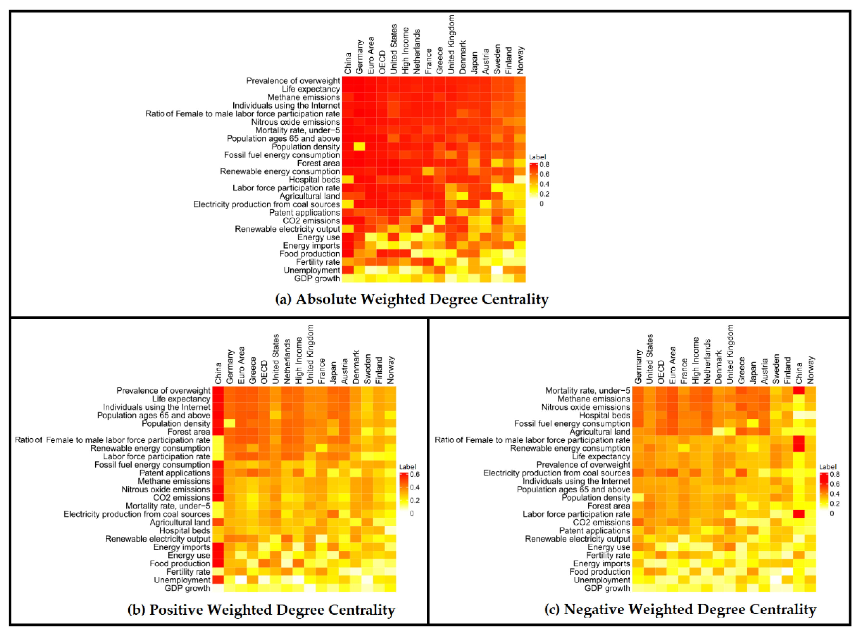
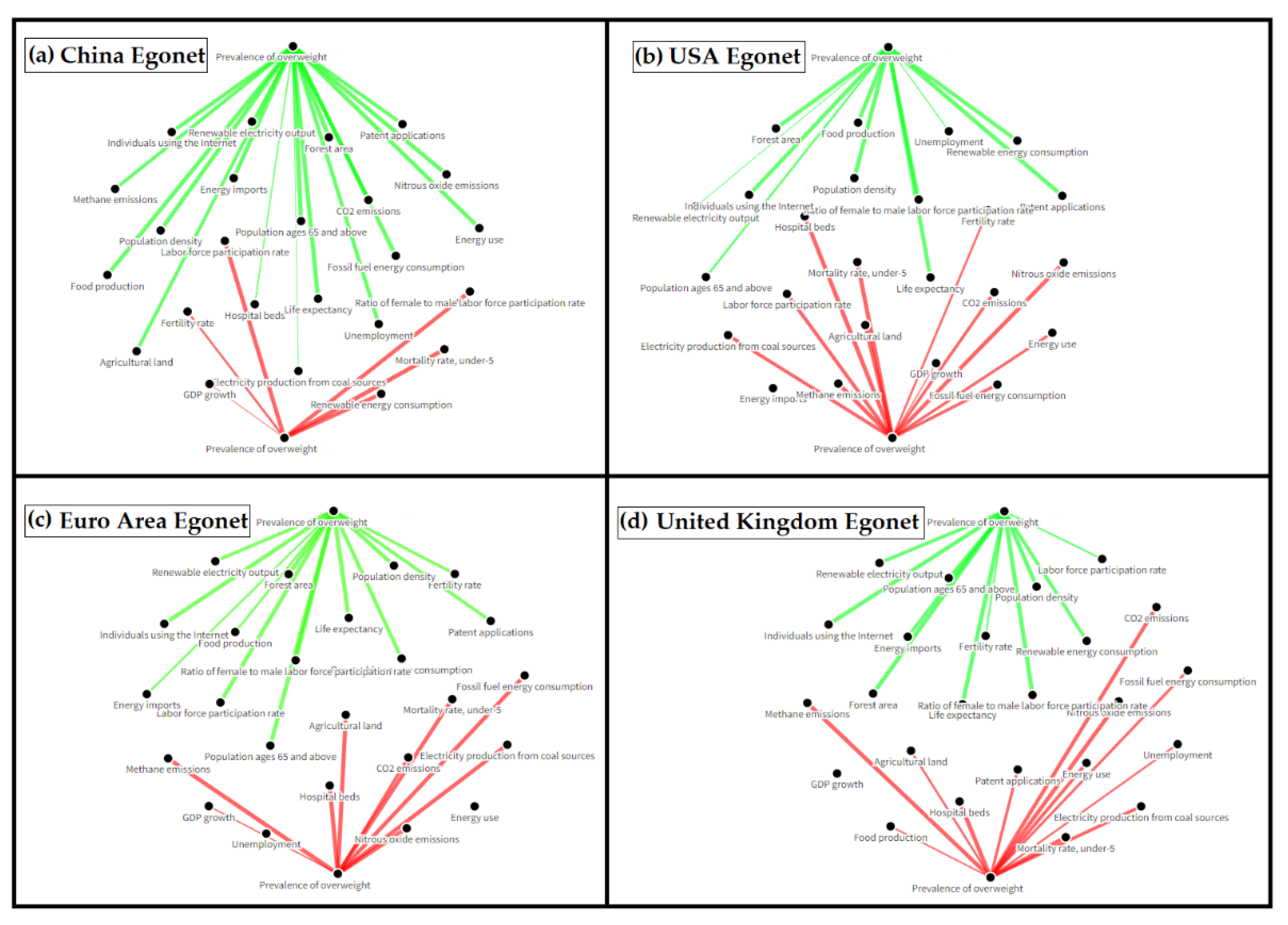
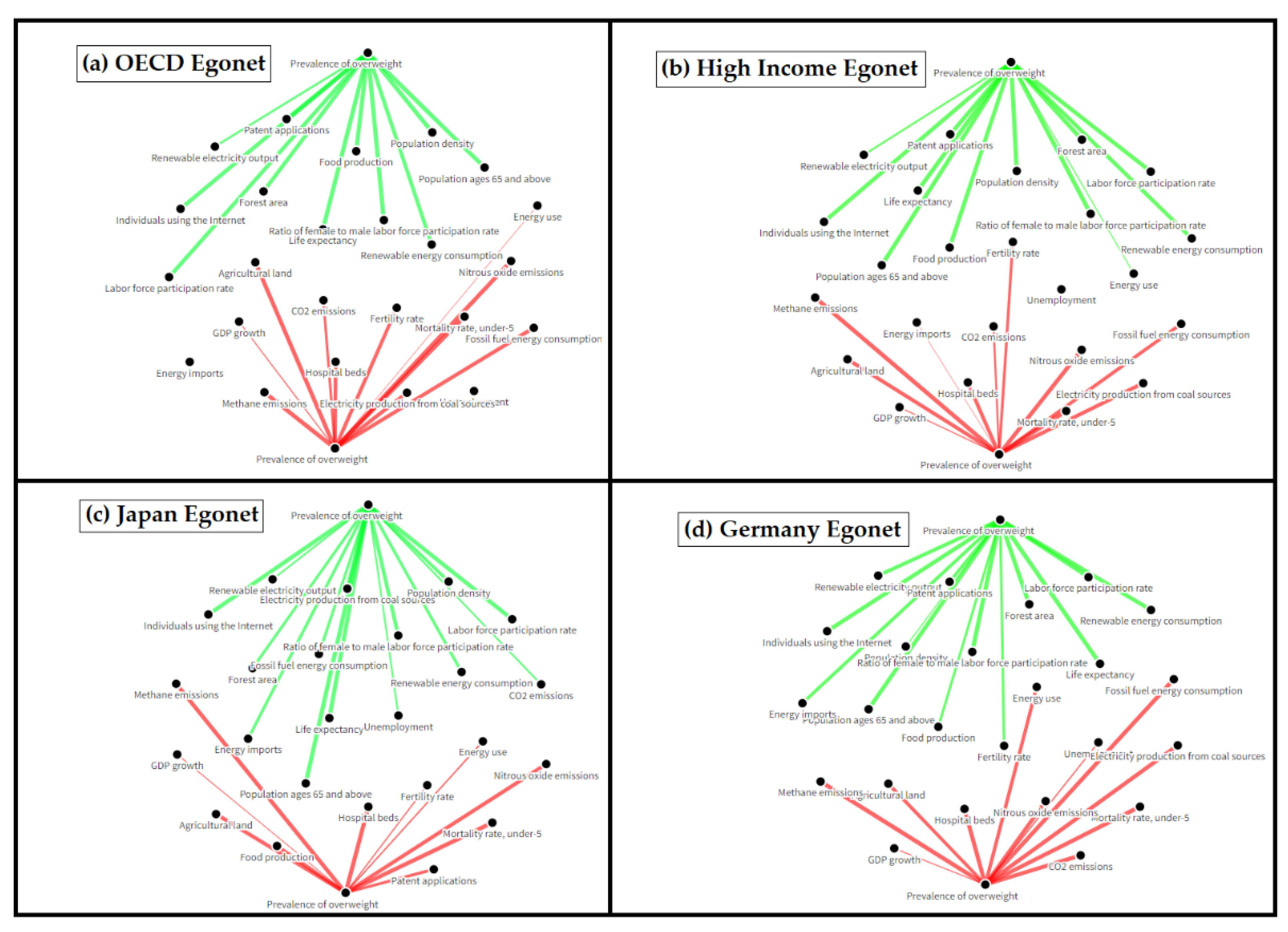
In this subsection, we are interested in identifying which ESG ratings are the most central, playing a key role, within ESG correlation networks. This research question is addressed, based on the degree centrality of the ESG indices (nodes), for all 16 economies examined. The resulting data are summarized and visualized in relevant heatmaps, for the case of (a) absolute, (b) positive, and (c) negative degree centrality. The key finding is that the ESG index, Prevalence of overweight, is the most central in all 16 economies examined. Therefore, we are interested in examining more closely the relevant egonets, aiming to identify with which nodes the correlation is positive or negative. We present indicatively the egonets for 8 economies: China, the USA, the Euro Area, the UK, the OECD, High Income, Japan, Germany. The remarks from local analysis are the following.

Remark 1. 

Prevalence of Overweight and Life Expectancy are the most central ESG ratings, while, unexpectedly, GDP Growth and Unemployment are at the bottom of the list.

Focusing on ESG indices, we can observe Figure 2 by rows. More specifically, from Figure 2a we observe that health-related ESG ratings are the most central nodes, in terms of absolute weighted degree centrality, in all 16 economies examined. The most central ESG ratings are: Prevalence of overweight and Life expectancy. In addition, other health-related ESG ratings with high centrality are: Population ages 65 and above and Mortality rate under-5. Concerning emissions, Methane emissions and Nitrous oxide emissions are central nodes for all 16 economies examined, while, on the contrary, CO₂ emissions is not always a central node. It is interesting to observe that the Ratio of female to male labor force participation rate, as well as the Individuals using the Internet are central nodes for all 16 economies examined. Concerning energy consumption, Fossil fuel energy consumption and Renewable energy consumption are central nodes for most of the economies examined.

Concerning low centrality nodes, it is striking to observe that two of the most commonly used economic indicators, namely GDP growth and Unemployment, are at the bottom of the list (Figure 2a). In the same direction, it is unexpected to observe that Energy use and Energy imports are also low centrality nodes, for most economies examined.

Remark 2. 

China has specific ESG ratings with remarkably high positive or high negative centrality. The existence of such “positive or negative hubs” was not observed in other economies examined.

Focusing on economies, we can observe Figure 2 by columns. More specifically, from Figure 2b we observe that China has specific ESG ratings with remarkably high positive centrality (positive hubs), as, for example: Prevalence of overweight, Life expectancy, Individuals using the Internet, Population ages 65 and above, Fossil fuel energy consumption, Patent applications, Energy imports, Energy use, and, surprisingly Unemployment. Similarly, from Figure 2c, we observe that specific ESG ratings have remarkably high negative centrality (negative hubs), as, for example: Ratio of Female to male labor force participation rate, Renewable energy consumption, Labor force participation rate, Mortality rate under-5. The existence of such “positive or negative hubs” was not observed in other economies examined. This different pattern for China may be understandable, as China’s economy has unique features, following a different path for development and social organization [56]. In addition, the growth rate of China’s economy has been about 8%, on average, since 1978 [57]. Moreover, both labor force participation rate and total factor productivity grew rapidly during this period [57].

Remark 3. 

Τhe most central ESG index, “Prevalence of Overweight”, is positively correlated with nodes “Individuals using the Internet” and “Ratio of female to male labor force participation rate”, in almost every economy examined.

From the egonets of Figure 3 and Figure 4, we observe that the Prevalence of Overweight is positively correlated with many ESG indices; for example, Life expectancy, Individuals using the internet, Ratio of female to male labor force participation rate and Population density. On the other hand, Mortality rate under-5, Methane emissions, Nitrous oxide emissions and Agricultural land are negatively correlated with Prevalence of Overweight. Generally speaking, in most economies, Prevalence of Overweight is positively correlated with 11 out of 24 ESG ratings, while, on the contrary, it is negatively correlated with 9 out of 24 ESG ratings (Appendix A, Egonets in Supplementary Material).

3.2. Global Analysis (Degree Centralization, Network Density, Network Balance)

In this subsection, we are interested in identifying which economies have the most centralized, or the densest, ESG correlation network. In other words, in this subsection, we are interested in the global characteristics of the ESG networks, as a whole. The above research question was addressed, based on degree centralization and network density, for all 16 economies examined. As the ESG correlation networks are signed (having both positive and negative weights), we are also interested in examining to what extent these networks are balanced, in the sense that they can be split into two negatively correlated groups of ESG ratings. This property in signed networks may have strong implications on hedging risk, if we see ESG ratings as underlying assets for portfolio selection [58,59,60,61,62,63,64,65]. The resulting data are summarized and visualized in relevant bar plots and heatmaps. The remarks from global analysis are the following.

Remark 4. 

China’s ESG correlation network has remarkably higher positive and negative centralization compared to other economies, with strong implications for its vulnerability and targeted controllability. Interestingly, if the sign of correlations is omitted, this result cannot be captured.

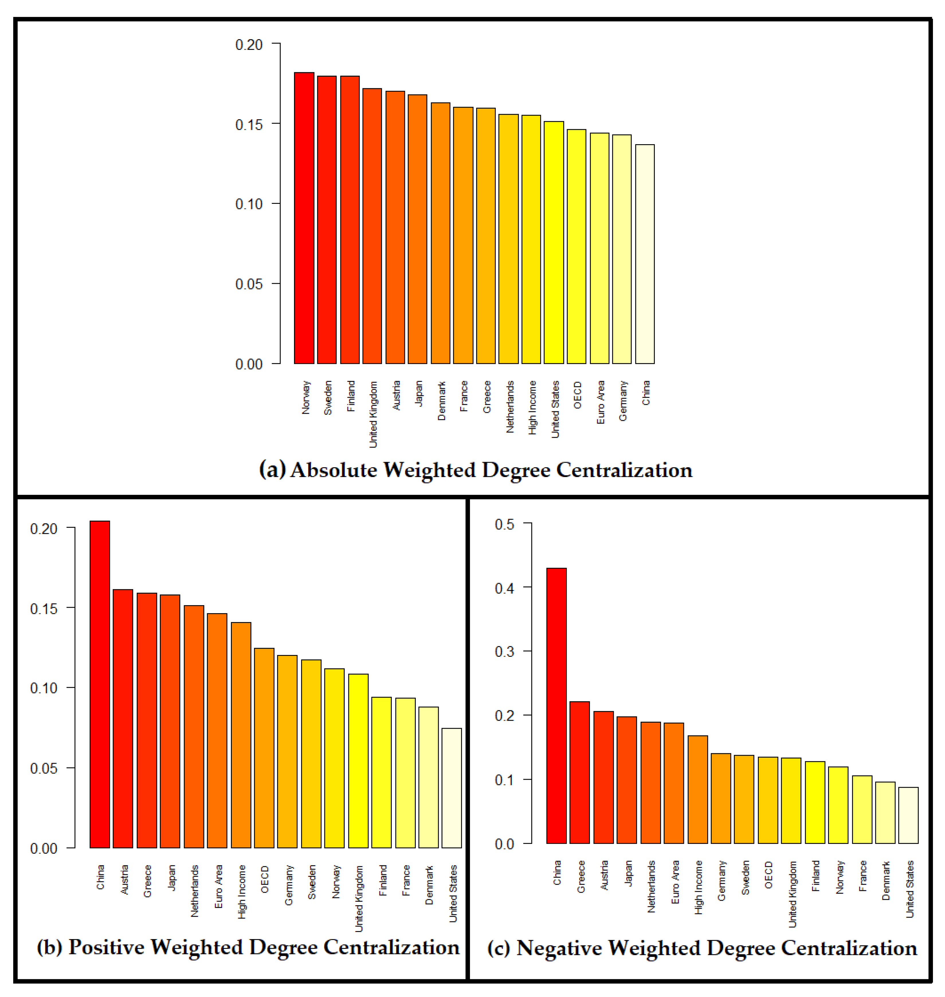
From Figure 5b,c, we observe that China’s ESG correlation network has remarkably higher positive and negative centralization, compared to other economies, which is understandable due to the existence of “positive and negative hubs” (Remark 2). This finding has strong implications for the vulnerability and targeted controllability of China’s ESG correlation network. A fundamental result in network theory is that the transmission of shocks, and therefore the vulnerability of the network, is related to structure, with centralized networks (in-homogeneously connected) being the most fragile [66]. In addition, it is well-known that centralized networks (heterogeneously connected) are target controllable [67]. In our context, this is understandable in the following way: targeted shocks, originating from positive and negative hubs, may propagate fluctuations to other nodes (ESG indices), resulting in the destabilization of the corresponding ESG network. Positive hubs control the network via positive correlations, while negative hubs control the network via negative correlations.

On the other hand, concerning economies with low centralization, the ESG correlation networks of France, Denmark and the USA have the lowest positive and negative centralization (Figure 5b,c). Thus, they are robust to targeted control and manipulation.

Interestingly, if the sign of correlations is omitted, the above result cannot be captured. More specifically, in Figure 5a, the centralization scores for all 16 economies are similar, with China at the bottom of the list. In other words, if the sign of correlations is omitted, valuable information may be lost. This is a clear example of why signed network analysis is needed, without leaving aside the sign of correlations. This is the key methodological novelty of our work compared to other analyses, especially in financial networks, where the sign of correlations is eliminated with mathematical tricks, like the similarity distance ${\mathrm{d}}_{\mathsf{\kappa }\mathsf{\lambda }}=\sqrt{2·\left(1-{\mathrm{c}}_{\mathsf{\kappa }\mathsf{\lambda }}\right),}$ which maps the values of the Pearson correlation coefficient ${\mathrm{c}}_{\mathsf{\kappa }\mathsf{\lambda }}\in \left[-1,1\right]$ to the non-negative interval ${\mathrm{d}}_{\mathsf{\kappa }\mathsf{\lambda }}\in \left[0,2\right]$ monotonically.

Remark 5. 

ESG correlation networks are quite dense. China has high positive density, which contributes further to the controllability of its ESG network.

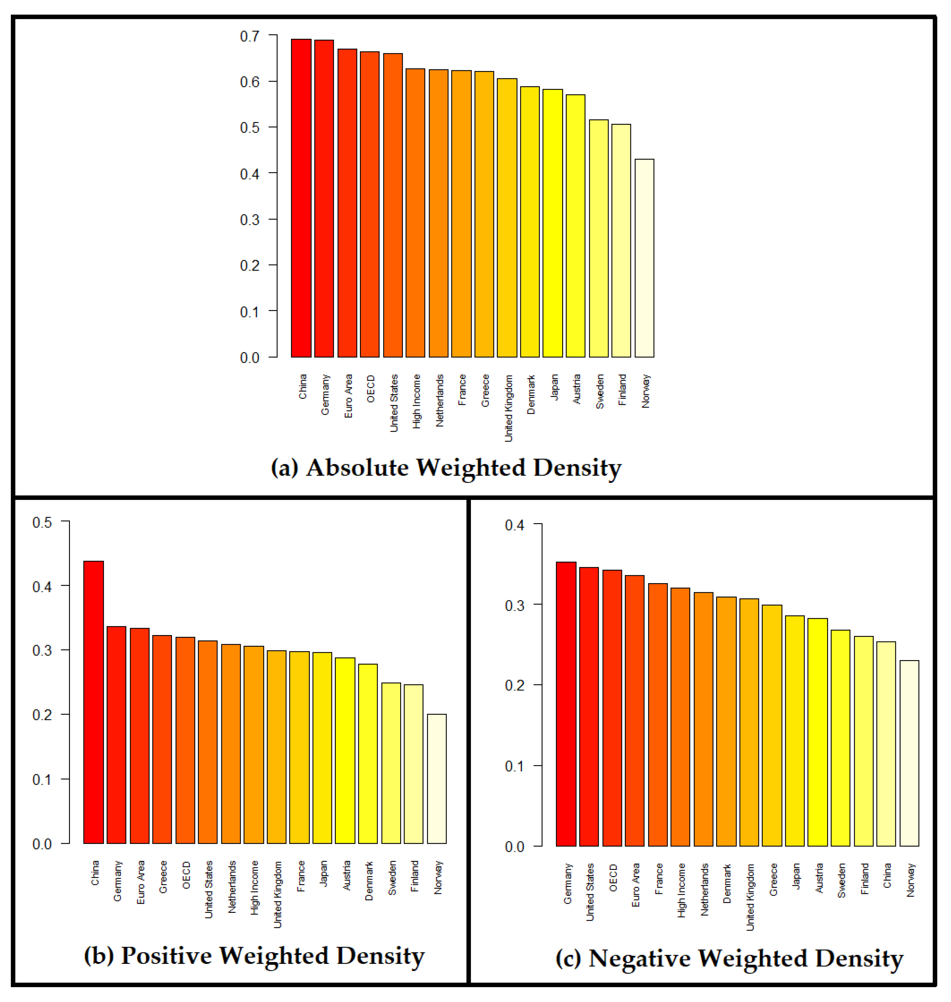
From Figure 6a, we observe that the ESG correlation networks are quite dense, for all 16 economies examined. This means that ESG ratings are significantly correlated with each other. This finding is stronger for China, Germany, the Euro Area, the OECD, the USA, and weaker for Scandinavian Countries (Sweden, Finland, Norway). For negative density, we observe that all economies have similar values (Figure 6c).

From Figure 6b, we observe that China has remarkably higher positive density compared to other economies, which means that many ESG ratings (nodes) are moving similarly towards the same direction. It is well-known that dense networks are more controllable [68]. Taking into account the discussion in Remark 4, this dense structure of positive correlations, makes the ESG network of China even more controllable.

It is interesting to note that, for the absolute weighted density (Figure 6a), the ordering of the 16 economies is the exact opposite of the ordering observed for the absolute weighted degree centralization (Figure 5a).

Remark 6. 

The ESG correlation networks are extremely balanced, i.e., they are split into two negatively correlated Groups of ESG ratings (nodes).

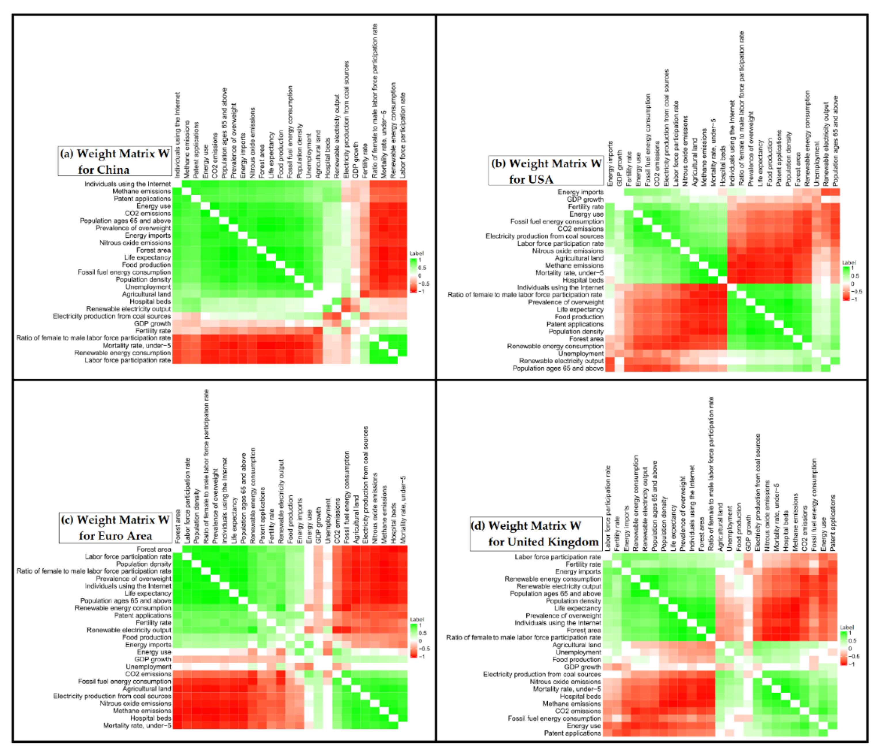
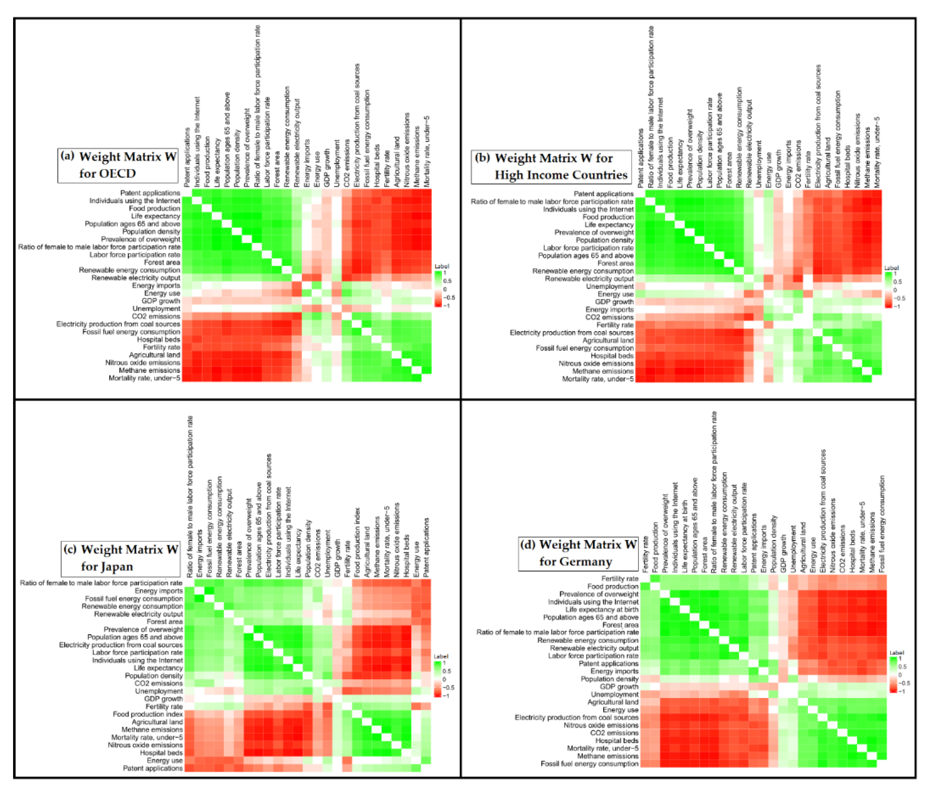
From Figure 7 and Figure 8, we observe that the ESG correlation networks are split into two negatively correlated groups of nodes. In other words, the intra-group weights are positive, while, on the contrary, the inter-group weights are negative. This finding was confirmed in all 16 economies examined (Weight Matrices in Supplementary Material). We specified the ESG ratings (nodes) of the two anti-correlated groups. For most of the economies examined, the first group (Group A) includes: Labor force participation rate, Prevalence of overweight, Life expectancy, Individuals using the Internet, Ratio of female to male labor force participation rate, Population density, Renewable energy consumption, Patent applications. The second anti-correlated group (Group B) includes: Mortality rate under 5, Methane emissions, Nitrous oxide emissions, Agricultural land, Fossil fuel energy consumption. More details about the two anti-correlated groups of ESG ratings (nodes) are presented in Appendix B.

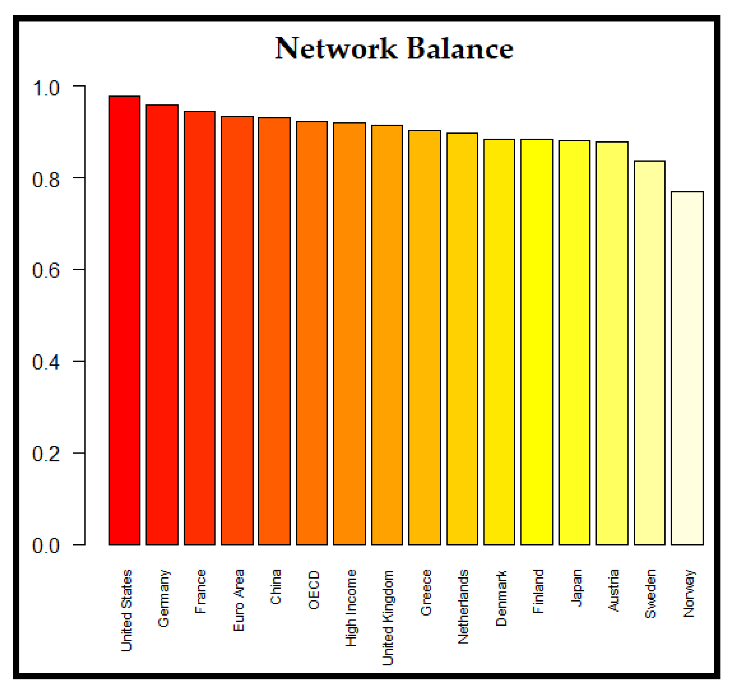
We quantify, with Frustration-based Balance (Definition 9) [53], how close the networks are to a perfect structural split of two anti-correlated groups of ESG ratings (nodes). The results are presented in Figure 9, where it is striking to observe that ESG correlation networks are extremely balanced, about 90%, on average, for all 16 economies examined. It is impressive that the USA’s network achieved almost perfect balance (97.9%, Figure 9), i.e., almost perfect structural split (Figure 7b). This split of network structure may have strong implications on hedging risk, if we see ESG ratings as underlying assets for portfolio selection. More specifically, investing into anti-correlated assets, called “hedge assets”, can be useful to offset potential losses [58,59,60,61,62,63,64,65].

4. Conclusions

The research purpose of this work was to provide the first analysis of correlation networks, constructed from ESG ratings of selected economies. We examined 25 ESG indices for 16 economies for a time period from 1990 to 2015. The ESG dataset was provided by the World Bank. For each economy, the relevant correlation network was constructed as follows: the ESG indices correspond to nodes, and the links between the nodes are signed weighted according to the Pearson correlation coefficient. We assessed the resulting correlation networks with selected metrics for individual nodes (local analysis), as well as for the network as a whole (global analysis).

Concerning local analysis, the main finding was that Prevalence of Overweight and Life Expectancy are the most central ESG ratings (Remark 1). Generally speaking, health-related ESG ratings are the most central nodes. On the other hand, it was striking to observe that two of the most commonly used economic indicators, namely GDP growth and Unemployment, are at the bottom of the list. Although at first these findings surprised us, after reviewing the relevant literature, we found that many studies emphasize the significance of a healthy workforce [69,70,71]. More specifically, there is a strong impact of obesity in labor productivity and health costs [72,73,74]. Considering the importance of the health factor, it has been proposed to add H to ESG, as H-ESG [75], and our findings seem to agree with this direction. In addition, ESG agencies, like MSCI, Beyond Ratings, and Sustainalytics, are also in accordance with our results: (a) Life Expectancy is one of the most important ESG indices, and (b) GDP growth has limited influence on the overall score of a country [19]. Another interesting result concerning Prevalence of Overweight is that it is positively correlated with nodes Individuals using the Internet and Ratio of female to male labor force participation rate in almost every economy examined (Remark 3). We make a special mention of the case of China, as the results of our analysis are slightly different, compared to those of other economies. China has specific ESG ratings with remarkably high positive or high negative centrality (Remark 2). The existence of such “positive or negative hubs” was not observed in other economies examined. The most notable example is Unemployment: while in all other economies the centrality of Unemployment is negligible, for China Unemployment is one of the most central nodes. This different result for China may be understandable, as China’s growth rate has been about 8%, on average, since 1978 [57], while additionally, the labor force participation rate and the total factor productivity grew rapidly during this period [57].

Concerning global analysis, we found that China’s network has remarkably higher positive and negative centralization compared to other economies (Remark 4), which is understandable of course, due to the existence of “positive and negative hubs”, mentioned above. It is important to note that this high centralization of China’s network, has strong implications on network vulnerability [66] and targeted controllability [67] in the following way: targeted shocks, originating from positive and negative hubs, may propagate fluctuations to other nodes (ESG indices), resulting in the destabilization of corresponding networks. Interestingly, if the sign of correlations is omitted, the above result cannot be captured. This is a clear example of why signed network analysis is needed, without leaving aside the sign of correlations. This is the key methodological novelty of our work. In addition to high centralization, we found that China’s network also has high positive density, which contributed further to the controllability [68] of its ESG network (Remark 5). Generally speaking, the ESG correlation networks are quite dense for all economies examined.

The most striking result of our analysis comes from global analysis, and concerns frustration-based Network Balance (Definition 9) [53]. As the ESG correlation networks are signed, having both positive and negative weights, we were interested in examining to what extent these networks were frustration-based balanced, in the sense that they can be split into two negatively correlated groups of nodes (ESG ratings). Surprisingly, we found that the ESG networks of all economies examined are extremely balanced, about 90% on average (Remark 6). It was impressive that the USA’s network achieved almost perfect balance (97.9%), i.e., almost perfect structural split. This split of network structure may have strong implications on hedging risk, if we see ESG ratings as underlying assets for portfolio selection. More specifically, investing into anti-correlated assets, called “hedge assets”, can be useful to offset potential losses [58,59,60,61,62,63,64,65]. Investigating further this structural split of ESG networks, we also specified the nodes (ESG ratings) of each anti-correlated group (Remark 6).

Our work provides new valuable insights concerning the structure of ESG correlation networks, by using signed weighted network analysis. Our future direction is to apply and extend the proposed signed network analysis to ESG ratings of corporate organizations, aiming to design optimal portfolios with desired balance between risk and return (greatest possible returns with acceptable risk or lowest risk given a certain return).

References

- Kenny, M.; Meadowcroft, J. Planning Sustainability, 2nd ed.; Routledge: London, UK, 2002. [Google Scholar]
- Artiach, T.; Lee, D.; Nelson, D.; Walker, J. The determinants of corporate sustainability performance. Account. Financ. 2010, 50, 31–51. [Google Scholar] [CrossRef]
- Governance & Accountability Institute. Sustainability Reports. Available online: https://www.ga-institute.com/fileadmin/ga_institute/images/FlashReports/2021/Russell-1000/G_A-Russell-Report-2021-Final.pdf?vgo_ee=NK5m02JiOOHgDiUUST7fBRwUnRnlmwiuCIJkd9A7F3A%3D (accessed on 12 August 2022).
- Amel-Zadeh, A.; Serafeim, G. Why and How Investors Use ESG Information: Evidence from a Global Survey. Financ. Anal. J. 2018, 74, 87–103. [Google Scholar] [CrossRef] [Green Version]
- Friede, G.; Busch, T.; Bassen, A. ESG and financial performance: Aggregated evidence from more than 2000 empirical studies. J. Sustain. Financ. Invest. 2015, 5, 210–233. [Google Scholar] [CrossRef] [Green Version]
- Duuren, E.v.; Plantinga, A.; Scholtens, B. ESG Integration and the Investment Management Process: Fundamental Investing Reinvented. J. Bus. Ethics 2016, 138, 525–533. [Google Scholar] [CrossRef] [Green Version]
- Fatemi, A.; Glaum, M.; Kaiser, S. ESG performance and firm value: The moderating role of disclosure. Glob. Financ. J. 2018, 38, 45–64. [Google Scholar] [CrossRef]
- Pedersen, L.H.; Fitzgibbons, S.; Pomorski, L. Responsible investing: The ESG-efficient frontier. J. Financ. Econ. 2021, 142, 572–597. [Google Scholar] [CrossRef]
- Principles for Responsible Investment. Available online: https://www.unpri.org/about-us/about-the-pri (accessed on 12 August 2022).
- Cerqueti, R.; Ciciretti, R.; Dalò, A.; Nicolosi, M. ESG investing: A chance to reduce systemic risk. J. Financ. Stab. 2021, 54, 100887. [Google Scholar] [CrossRef]
- Nofsinger, J.; Varma, A. Socially responsible funds and market crises. J. Bank. Financ. 2014, 48, 180–193. [Google Scholar] [CrossRef]
- Becchetti, L.; Ciciretti, R.; Dalò, A.; Herzel, S. Socially responsible and conventional investment funds: Performance comparison and the global financial crisis. Appl. Econ. 2015, 47, 2541–2562. [Google Scholar] [CrossRef]
- Nakai, M.; Yamaguchi, K.; Takeuchi, K. Can SRI funds better resist global financial crisis? Evidence from Japan. Int. Rev. Financ. Anal. 2016, 48, 12–20. [Google Scholar] [CrossRef]
- Hübel, B. Do markets value ESG risks in sovereign credit curves? Q. Rev. Econ. Financ. 2020, 85, 134–148. [Google Scholar] [CrossRef]
- Tang, M. Did ESG Ratings Help to Explain Changes in Sovereign CDS Spreads? MSCI Issue Brief 2017. Available online: https://www.msci.com/documents/10199/6d12ed0d-814a-4d36-a152-e8c4f175ad67 (accessed on 1 November 2022).
- Capelle-Blancard, G.; Crifo, P.; Diaye, M.-A.; Oueghlissi, R.; Scholtens, B. Sovereign bond yield spreads and sustainability: An empirical analysis of OECD countries. J. Bank. Financ. 2019, 98, 156–169. [Google Scholar] [CrossRef]
- Crifo, P.; Diaye, M.-A.; Oueghlissi, R. The effect of countries’ ESG ratings on their sovereign borrowing costs. Q. Rev. Econ. Financ. 2017, 66, 13–20. [Google Scholar] [CrossRef]
- Berg, F.; Kölbel, J.F.; Rigobon, R. Aggregate Confusion: The Divergence of ESG Ratings. Forthcom. Rev. Financ. 2019. [Google Scholar] [CrossRef]
- Bouyé, E.; Menville, D. The Convergence of Sovereign Environmental, Social and Governance Ratings. In Policy Research Working Paper; No. 9583; World Bank: Washington, DC, USA, 2021; Available online: https://openknowledge.worldbank.org/handle/10986/35291 (accessed on 1 November 2022).
- Newman, M.E.J. Networks, 2nd ed.; Oxford University Press: Oxford, UK, 2018. [Google Scholar]
- Lusseau, D.; Mancini, F. Income-based variation in Sustainable Development Goal interaction networks. Nat. Sustain. 2019, 2, 242–247. [Google Scholar] [CrossRef] [Green Version]
- Dawes, J.H. SDG interlinkage networks: Analysis, robustness, sensitivities, and hierarchies. World Dev. 2022, 149, 105693. [Google Scholar] [CrossRef]
- Barro, D.; Basso, A. Credit contagion in a network of firms with spatial interaction. Eur. J. Oper. Res. 2010, 205, 459–468. [Google Scholar] [CrossRef] [Green Version]
- Billio, M.; Getmansky, M.; Lo, A.W.; Pelizzon, L. Econometric measures of connectedness and systemic risk in the finance and insurance sectors. J. Financ. Econ. 2012, 104, 535–559. [Google Scholar] [CrossRef]
- Loepfe, L.; Cabrales, A.; Sánchez, A. Towards a Proper Assignment of Systemic Risk: The Combined Roles of Network Topology and Shock Characteristics. PLoS ONE 2013, 8, e77526. [Google Scholar] [CrossRef] [PubMed] [Green Version]
- Elliott, M.; Golub, B.; Jackson, M.O. Financial Networks and Contagion. Am. Econ. Rev. 2014, 104, 3115–3153. [Google Scholar] [CrossRef]
- Moghadam, H.; Mohammadi, T.; Kashani, M.; Shakeri, A. Complex networks analysis in Iran stock market: The application of centrality. Phys. A Stat. Mech. Its Appl. 2019, 531, 121800. [Google Scholar] [CrossRef]
- Chabot, M. Financial stability indices and financial network dynamics in Europe. Rev. Économique 2021, 72, 591–631. [Google Scholar] [CrossRef]
- Fornito, A.; Zalesky, A.; Bullmore, E. Fundamentals of Brain Network Analysis, 1st ed.; Academic Press: Cambridge, MA, USA, 2016. [Google Scholar]
- U.N. General Assembly. Transforming Our World: The 2030 Agenda for Sustainable Development 2015. Available online: https://sdgs.un.org/2030agenda (accessed on 5 November 2022).
- International Council for Science (ICSU); International Social Science Council (ISSC). Review of the Sustainable Development Goals: The Science Perspective; International Council for Science (ICSU): Paris, France, 2015; ISBN 978-0-930357-97-9. Available online: https://council.science/wp-content/uploads/2017/05/SDG-Report.pdf (accessed on 1 November 2022).
- Nilsson, M.; Griggs, D.; Visbeck, M. Policy: Map the interactions between Sustainable Development Goals. Nature 2016, 534, 320–322. [Google Scholar] [CrossRef] [Green Version]
- Independent Group of Scientists appointed by the Secretary-General. Global Sustainable Development Report 2019: The Future is Now–Science for Achieving Sustainable Development; United Nations: New York, NY, USA, 2019; Available online: https://sustainabledevelopment.un.org/content/documents/24797GSDR_report_2019.pdf (accessed on 1 November 2022).
- Le Blanc, D. Towards Integration at Last? The Sustainable Development Goals as a Network of Targets. Sustain. Dev. 2015, 23, 176–187. [Google Scholar] [CrossRef]
- Weitz, N.; Carlsen, H.; Nilsson, M.; Skånberg, K. Towards systemic and contextual priority setting for implementing the 2030 Agenda. Sustain. Sci. 2018, 13, 531–548. [Google Scholar] [CrossRef] [Green Version]
- Allen, C.; Metternicht, G.; Wiedmann, T. Prioritising SDG targets: Assessing baselines, gaps and interlinkages. Sustain. Sci. 2019, 14, 421–438. [Google Scholar] [CrossRef]
- Zhou, X.; Moinuddin, M. Sustainable Development Goals Interlinkages and Network Analysis a Practical Tool for SDG Integration and Policy Coherence; Institute for Global Environmental Strategies (IGES): Kanagawa, Japan, 2017; Available online: https://www.iges.or.jp/en/publication_documents/pub/researchreport/en/6026/IGES_Research+Report_SDG+Interlinkages_Publication.pdf (accessed on 1 November 2022).
- Sebestyén, V.; Bulla, M.; Rédey, Á.; Abonyi, J. Network model-based analysis of the goals, targets and indicators of sustainable development for strategic environmental assessment. J. Environ. Manag. 2019, 238, 126–135. [Google Scholar] [CrossRef]
- Putra, M.P.I.F.; Pradhan, P.; Kropp, J.P. A systematic analysis of Water-Energy-Food security nexus: A South Asian case study. Sci. Total Environ. 2020, 728, 138451. [Google Scholar] [CrossRef]
- Jing, Z.; Wang, J. Sustainable development evaluation of the society–economy–environment in a resource-based city of China: A complex network approach. J. Clean. Prod. 2020, 263, 121510. [Google Scholar] [CrossRef]
- Swain, R.B.; Ranganathan, S. Modeling interlinkages between sustainable development goals using network analysis. World Dev. 2021, 138, 105136. [Google Scholar] [CrossRef]
- Ospina-Forero, L.; Castañeda, G.; Guerrero, O.A. Estimating networks of sustainable development goals. Inf. Manag. 2022, 59, 103342. [Google Scholar] [CrossRef]
- Dörgő, G.; Sebestyén, V.; Abonyi, J. Evaluating the Interconnectedness of the Sustainable Development Goals Based on the Causality Analysis of Sustainability Indicators. Sustainability 2018, 10, 3766. [Google Scholar] [CrossRef] [Green Version]
- Laumann, F.; von Kügelgen, J.; Uehara, T.H.K.; Barahona, M. Complex interlinkages, key objectives, and nexuses among the Sustainable Development Goals and climate change: A network analysis. Lancet Planet. Health 2022, 6, 422–430. [Google Scholar] [CrossRef]
- World Bank. Available online: https://databank.worldbank.org/source/environment-social-and-governance?preview=on (accessed on 12 August 2022).
- Knuth, D. Two Notes on Notation. Am. Math. Mon. 1992, 99, 403–422. [Google Scholar] [CrossRef]
- Freeman, L. Centrality in social networks conceptual clarification. Soc. Netw. 1978, 1, 215–239. [Google Scholar] [CrossRef] [Green Version]
- Heider, F. Attitudes and Cognitive Organization. J. Psychol. 1946, 21, 107–112. [Google Scholar] [CrossRef] [PubMed]
- Heider, F. The Psychology of Interpersonal Relations, 1st ed.; Lawrence Erlbaum Associates: Mahwah, NJ, USA, 1958. [Google Scholar]
- Harary, F. On the notion of balance of a signed graph. Mich. Math. J. 1953, 2, 143–146. [Google Scholar] [CrossRef]
- Cartwright, D.; Harary, F. Structural balance: A generalization of Heider’s theory. Psychol. Rev. 1956, 63, 277–293. [Google Scholar] [CrossRef] [Green Version]
- Facchetti, G.; Iacono, G.; Altafini, C. Computing global structural balance in large-scale signed social networks. Proc. Natl. Acad. Sci. USA 2011, 108, 20953–20958. [Google Scholar] [CrossRef] [Green Version]
- Aref, S.; Wilson, M. Measuring partial balance in signed networks. J. Complex Netw. 2018, 6, 566–595. [Google Scholar] [CrossRef]
- Signnet Package in R. Available online: https://cran.r-project.org/web/packages/signnet/index.html (accessed on 12 August 2022).
- CRAN. Available online: https://cran.r-project.org/ (accessed on 12 August 2022).
- Breslin, S. The ‘China model’ and the global crisis: From Friedrich List to a Chinese mode of governance? Int. Aff. 2011, 87, 1323–1343. [Google Scholar] [CrossRef] [Green Version]
- Zhu, X. Understanding China’s Growth: Past, Present, and Future. J. Econ. Perspect. 2012, 26, 103–124. [Google Scholar] [CrossRef] [Green Version]
- Baur, D.G.; McDermott, T.K. Is gold a safe haven? International evidence. J. Bank. Financ. 2010, 34, 1886–1898. [Google Scholar] [CrossRef]
- Reboredo, J.C. Is gold a hedge or safe haven against oil price movements? Resour. Policy 2013, 38, 130–137. [Google Scholar] [CrossRef]
- Baur, D.G.; Lucey, B.M. Is Gold a Hedge or a Safe Haven? An Analysis of Stocks, Bonds and Gold. Financ. Rev. 2010, 45, 217–229. [Google Scholar] [CrossRef]
- Hood, M.; Malik, F. Is gold the best hedge and a safe haven under changing stock market volatility? Rev. Financ. Econ. 2013, 22, 47–52. [Google Scholar] [CrossRef]
- Hillier, D.; Draper, P.; Faff, R. Do Precious Metals Shine? An Investment Perspective. Financ. Anal. J. 2006, 62, 98–106. [Google Scholar] [CrossRef]
- Dyhrberg, A.H. Hedging capabilities of bitcoin. Is it the virtual gold? Financ. Res. Lett. 2016, 16, 139–144. [Google Scholar] [CrossRef] [Green Version]
- Bouri, E.; Molnár, P.; Azzi, G.; Roubaud, D.; Hagfors, L.I. On the hedge and safe haven properties of Bitcoin: Is it really more than a diversifier? Financ. Res. Lett. 2017, 20, 192–198. [Google Scholar] [CrossRef]
- Ratner, M.; Chiu, C.C. Hedging stock sector risk with credit default swaps. Int. Rev. Financ. Anal. 2013, 30, 18–25. [Google Scholar] [CrossRef]
- Albert, R.; Jeong, H.; Barabási, A.L. Error and attack tolerance of complex networks. Nature 2000, 406, 378–382. [Google Scholar] [CrossRef] [PubMed] [Green Version]
- Gao, J.; Liu, Y.-Y.; D’Souza, R.; Barabási, A.-L. Target control of complex networks. Nat. Commun. 2014, 5, 5415. [Google Scholar] [CrossRef] [PubMed] [Green Version]
- Liu, Y.-Y.; Slotine, J.-J.; Barabási, A.-L. Controllability of complex networks. Nature 2011, 473, 167–173. [Google Scholar] [CrossRef]
- Henke, R.M.; Carls, G.S.; Short, M.E.; Pei, X.; Wang, S.; Moley, S.; Sullivan, M.; Goetzel, R.Z. The Relationship Between Health Risks and Health and Productivity Costs Among Employees at Pepsi Bottling Group. J. Occup. Environ. Med. 2010, 52, 519–527. [Google Scholar] [CrossRef]
- Fabius, R.; Phares, S. Companies That Promote a Culture of Health, Safety, and Wellbeing Outperform in the Marketplace. J. Occup. Enviromental Med. 2021, 63, 456–461. [Google Scholar] [CrossRef]
- Henke, R.M.; Goetzel, R.Z.; McHugh, J.; Isaac, F. Recent Experience In Health Promotion At Johnson & Johnson: Lower Health Spending, Strong Return On Investment. Health Aff. 2011, 30, 490–499. [Google Scholar] [CrossRef]
- Okunogbe, A.; Nugent, R.; Spencer, G.; Ralston, J.; Wilding, J. Economic impacts of overweight and obesity: Current and future estimates for eight countries. BMJ Glob. Health 2021, 6, e006351. [Google Scholar] [CrossRef]
- Mazhar, U.; Rehman, F. Productivity, obesity, and human capital: Panel data evidence. Econ. Hum. Biol. 2022, 44, 101096. [Google Scholar] [CrossRef]
- Goettler, A.; Grosse, A.; Sonntag, D. Productivity loss due to overweight and obesity: A systematic review of indirect costs. BMJ Open 2017, 7, e014632. [Google Scholar] [CrossRef]
- Williams, M.; Geli, P. ESG is not enough. It’s time to add an H. Fortune. 14 March 2022. Available online: https://fortune.com/2022/03/14/esg-is-not-enough-time-to-add-health-wellbeing-csr-workers-pandemic-leadership-geli-williams/ (accessed on 1 November 2022).
Figure 1.
Illustration of a balanced (left) and an unbalanced (right) network. The left network (a) is balanced because it is structurally split into two groups, where all intra-group weights are positive and all inter-group weights are negative. On the contrary, the right network (b) is not balanced due to three “frustrated” links, namely: 1–2 (negative intra-group link), 7–9 (negative intra-group link), and 5–6 (positive inter-group link).
Figure 2.
Heatmaps illustrating the Degree Centrality of the 25 ESG indices (nodes) for the 16 economies, in case of: (a) absolute weight matrix , (b) positive weight matrix , and (c) negative weight matrix .
Figure 3.
Egonets of ESG index Prevalence of overweight illustrating the positive and negative correlations with other ESG indices, based on weight matrix , in case of: (a) China, (b) USA, (c) Euro Area, (d) United Kingdom.
Figure 4.
Egonets of ESG index Prevalence of overweight illustrating the positive and negative correlations with other ESG indices, based on weight matrix , in case of: (a) OECD, (b) High Income, (c) Japan, (d) Germany.
Figure 5.
Bar plots illustrating the Degree Centralization of the ESG correlation networks for the 16 economies, in case of: (a) absolute weight matrix , (b) positive weight matrix , and (c) negative weight matrix .
Figure 6.
Barplots illustrating the Density of the ESG correlation networks for the 16 economies, in case of: (a) absolute weight matrix , (b) positive weight matrix , and (c) negative weight matrix .
Figure 7.
Heatmaps illustrating the positive and negative correlations among the 25 ESG indices (nodes), based on weight matrix , in case of: (a) China, (b) USA, (c) Euro Area, (d) United Kingdom.
Figure 8.
Heatmaps illustrating the positive and negative correlations among the 25 ESG indices (nodes), based on weight matrix , in case of: (a) OECD, (b) High Income, (c) Japan, (d) Germany.
Figure 9.
Bar plot illustrating the Frustration-based Balance of the ESG correlation networks for the 16 economies, based on weight matrix .