Failure Prediction for the Tearing of a Pin-Loaded Dual Phase Steel (DP980) Adjusting Guide


1
Department of Automotive and Mechanical Engineering, Kongju National University, Cheonan 31080, Korea
2
Seat R&D Center, Hyundai Transys, 174, Yeongcheon-ro, Hwaseong-si, Gyeonggi-do 18463, Korea
*
Author to whom correspondence should be addressed.
Appl. Sci. 2019, 9(24), 5460; https://doi.org/10.3390/app9245460
Submission received: 14 November 2019
/
Revised: 6 December 2019
/
Accepted: 6 December 2019
/
Published: 12 December 2019
(This article belongs to the Special Issue Selected Papers from the ICMR 2019)
Abstract
:Owing to their outstanding strength, in recent years, there has been an increased use of advanced high-strength steel (AHSS) sheets in the automotive sector. Their low formability, however, poses a challenge to forming, and failure prediction requires accurate knowledge of its material behavior over a large strain range up to ultimate failure, in order to exploit their full capacity in forming, but also in crash events. For predicting the fracture of an adjusting guide loaded by a pin, first, the force–displacement data are extracted from tensile tests using DP980 specimens of diverse shapes, all of which represent a certain loading mode. Using digital image correlation (DIC), we determine the stress triaxialities corresponding to the diverse loading conditions and establish the triaxiality failure diagram (TFD), which serves as the basis for the generalized incremental stress state-dependent damage model (GISSMO). Then, the damage parameters (necking and failure strains) are determined for each loading mode by reverse engineering-based optimization. Finally, these damage parameters are applied to the adjusting guide, and the numerical results are compared with the experimental data. Comparisons of the external load–displacement curves and the local equivalent strain distributions show that using the damage model with the material parameters obtained in here allows for the accurate prediction of the guide’s failure behavior, and the applicability of GISSMO to complex loading cases.
1. Introduction
As an efficient means to reduce weight and increase safety, advanced high-strength steel (AHSS) sheets have become widespread in the automotive industry. The AHSS used here, DP980, is a dual phase steel consisting of a soft ferrite matrix containing tough islands of mainly martensite. Due to its very high strength of at least 980 MPa, good strength-to-weight ratio, and low cost but still relatively good formability, it has become an attractive sheet material for automobile components such as bumpers. However, its rather low elongation to failure poses a challenge to forming, and accurate knowledge of their deformation behavior—in particular, that between incipient necking and failure—is thus of paramount importance in order to exploit its full potential.
Numerous ductile damage models have been developed over the past decades. They can be categorized into micromechanics-based (e.g., the maximum stress-based Cockcroft–Latham model [1], its modification by Oh et al. [2], the volumetric strain limit-based model by Oyane [3], the porous plasticity-based Gurson model [4], the monotonic function-based Johnson–Cook model [5], which is in this regard similar to the older McClintock [6] and Rice–Tracey [7] models) and phenomenological models (e.g., Bai–Wierzbicki [8] and generalized incremental stress state-dependent damage model (GISSMO) [9]). All recent models have in common that the fracture strain, εf, is considered a function of triaxiality, η, defined as the ratio of mean stress to equivalent stress. Models differ by the shape of the εf-η function (exponential, polynomial, mixed functions, etc.) and the number of additional variables (Lode angle, strain rate, and temperature) and fitting coefficients. Generally, the accuracy of these models increases with the number of coefficients and variables. Still, these models are deficient, as they cannot accurately cover a larger range of triaxiality (e.g., Cockcroft–Latham), may falsely predict fracture for other triaxialities, cannot handle strain path changes, are linked to a certain constitutive model, cannot account for shear-dominated failure (e.g., Gurson model), cannot handle non-linear damage growth, and cannot tackle the problem of mesh-dependence arising in numerical simulations once strains become close to the fracture limit.
In a phenomenological model, the generalized incremental stress state-dependent damage model (GISSMO) meets many of these demands in an elegant and straightforward manner by tabulating εf-η data, and thus allowing for any triaxiality failure diagram (TFD) shape [10]. It has consequently been developed, integrated into the commercial finite element (FE) code LS-Dyna [11], and successfully applied to structures under diverse loading scenarios (e.g., [12]). However, there is still a lack of validation examples. Furthermore, η was often not determined experimentally, but assumed based on finite element analysis or theory.
In this study, we attempted to predict the failure through the tearing of an adjusting guide loaded by a pin. To do so, we obtained force–displacement data for diverse stress states, represented through stress triaxiality, η, induced in the material by using diverse specimens (shear, uniaxial tension, and notch specimens). For the local strain measurement, especially for the post-necking region, digital image correlation (DIC) was employed, and representative η-values corresponding to the single specimen types were calculated from the strain fields. Damage was accounted for by applying GISSMO; the damage parameters were obtained through reverse engineering-based optimization with the commercial graphical optimization tool LS-Opt. These material parameters were then applied to the numerical adjusting guide model of a passenger vehicle, and finally, the damage parameters were validated by comparing the experimental external force–displacement (FD) data, as well as the equivalent strain distributions from the adjusting guide tearing test with the numerical results. DIC was employed again to compare the local equivalent strain distributions.
2. Damage Model and Local Strain Measurement
In this section, the DIC method for displacement and strain full field measurements, and the damage model used to account for the material deterioration at higher strains are introduced.
2.1. Digital Image Correlation (DIC)
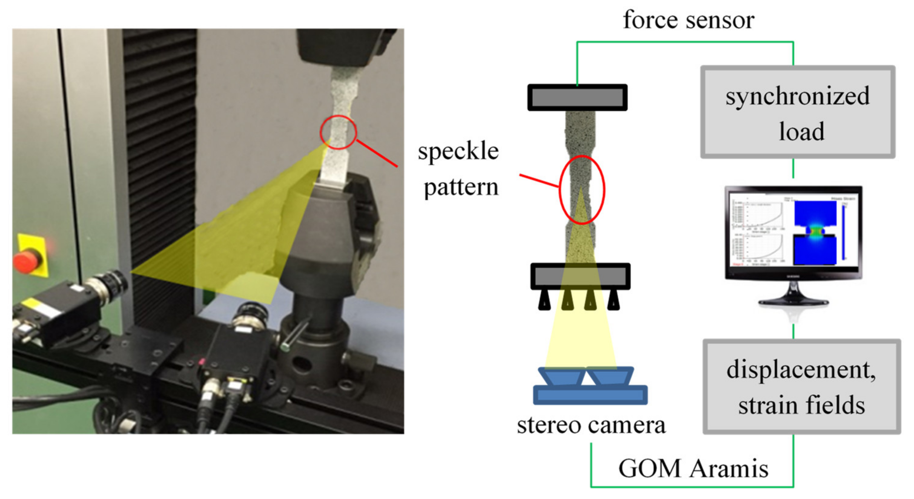
To determine the distribution of η in the specimen center and to extract its representative value, the local displacement and strain distributions were measured optically using DIC. The test setup is shown in Figure 1. Prior to the test, an irregular, high-contrast speckle pattern was sprayed onto the specimen surface. The pattern was then recorded during the test using a stereo camera (resolution 1280 × 1024 pixels) with one frame per second, and after the test, the pattern changes were converted to displacements and strains in GOM (Gesellschaft für Optische Messtechnik mbH) Aramis Professional (2019) [13].
2.2. Triaxiality Failure Diagram and GISSMO
GISSMO is an isotropic phenomenological damage model and can be regarded as a very straightforward and pragmatic approach towards the prediction of damage, and accounts for shear-dominated failure [9]. In the GISSMO framework, the equivalent strains at the onset of necking, εu, and at fracture, εf, are treated as stress triaxiality η-dependent weight functions in the calculation of the forming intensity, F, and damage parameter, D, as follows:
where i and i + 1 denote the previous and the current FE analysis step, respectively. In LS-Dyna, the initial F is set to 10−20, so as to allow for the evolution of F. εeq denotes the equivalent plastic strain (“equivalent” in a von Mises sense), and η represents the stress state. For plane stress conditions, as is the case for thin sheets, η is limited to (−2/3, 2/3), and is defined as follows:
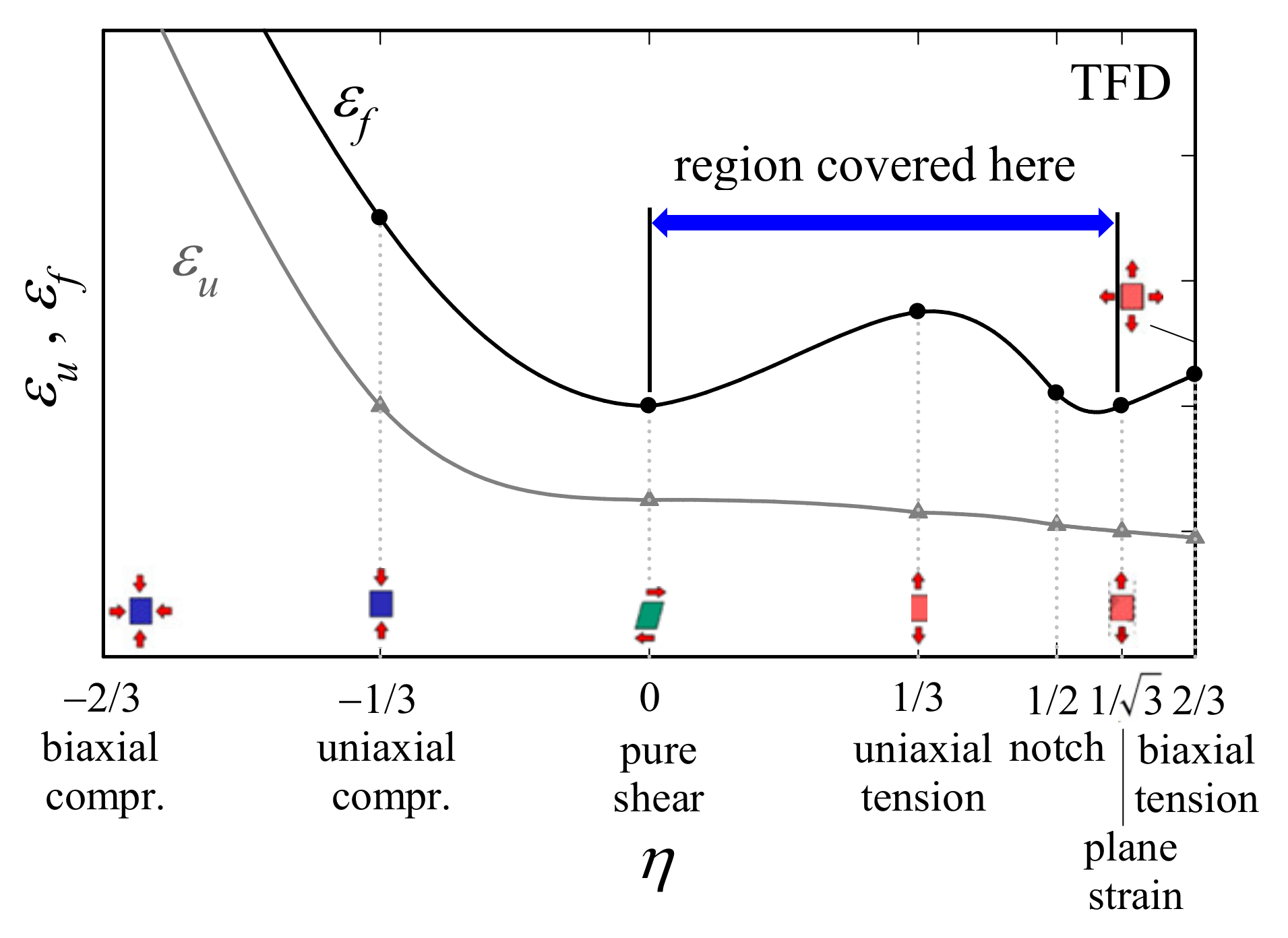
where σm, σeq, σ1, and σ2 are the mean stress, equivalent stress (here in a von Mises sense), and maximum and minimum principal in-plane stresses, respectively. Note that while εu and εf are triaxiality-dependent material properties, there was only one set of m and f that was found. The variations of εu and εf with η were provided by the TFD, as schematically shown in Figure 2. It is worth noting that the shapes of the curves are material-dependent; the run between two points is unknown. A further parameter, m (≥1), the damage evolution exponent, governs the shape of the damage accumulation law. For m = 1, Equation (1) reduces to the linear damage evolution proposed by Johnson and Cook, and with increasing m, we approach the Gurson model.
Once Fnew reaches unity, which is tantamount to the onset of diffuse necking, the corresponding Dnew, calculated by Equation (2), is assigned (Dc), and upon further loading, the stress tensor, σ, is reduced according to the following:
Equation (4) implies that the material weakens equally in all directions, and thus remains isotropic. For further fitting and mesh regularization, which are necessary in order to tackle the problem of mesh-dependence in the post-critical region, the fading exponent (f) was introduced. For f = 1 and Dc = 0, we arrived at the classical Lemaitre definition of the effective stress tensor. As can be seen from Equation (2), D starts becoming non-zero with the onset of yielding, and although D = (0, 1) still holds, D > 0 no longer necessarily means that the material’s performance has deteriorated (but D > Dc). However, D = 1 still indicates failure. To mitigate the problem of mesh-dependence, the GISSMO parameters were made characteristic element length (e)-dependent through the regularization of the energy dissipation in the post-critical region [14]. For this, tensile tests were simulated with various e, and the numerical force–displacement (FD) results were fitted to the experimental FD data.
3. Determination of Flow and Damage Properties
3.1. Tensile Testing
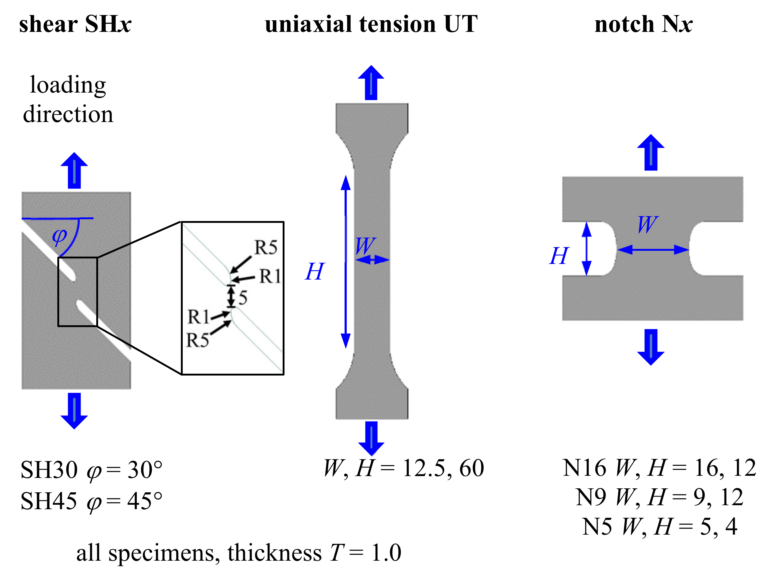
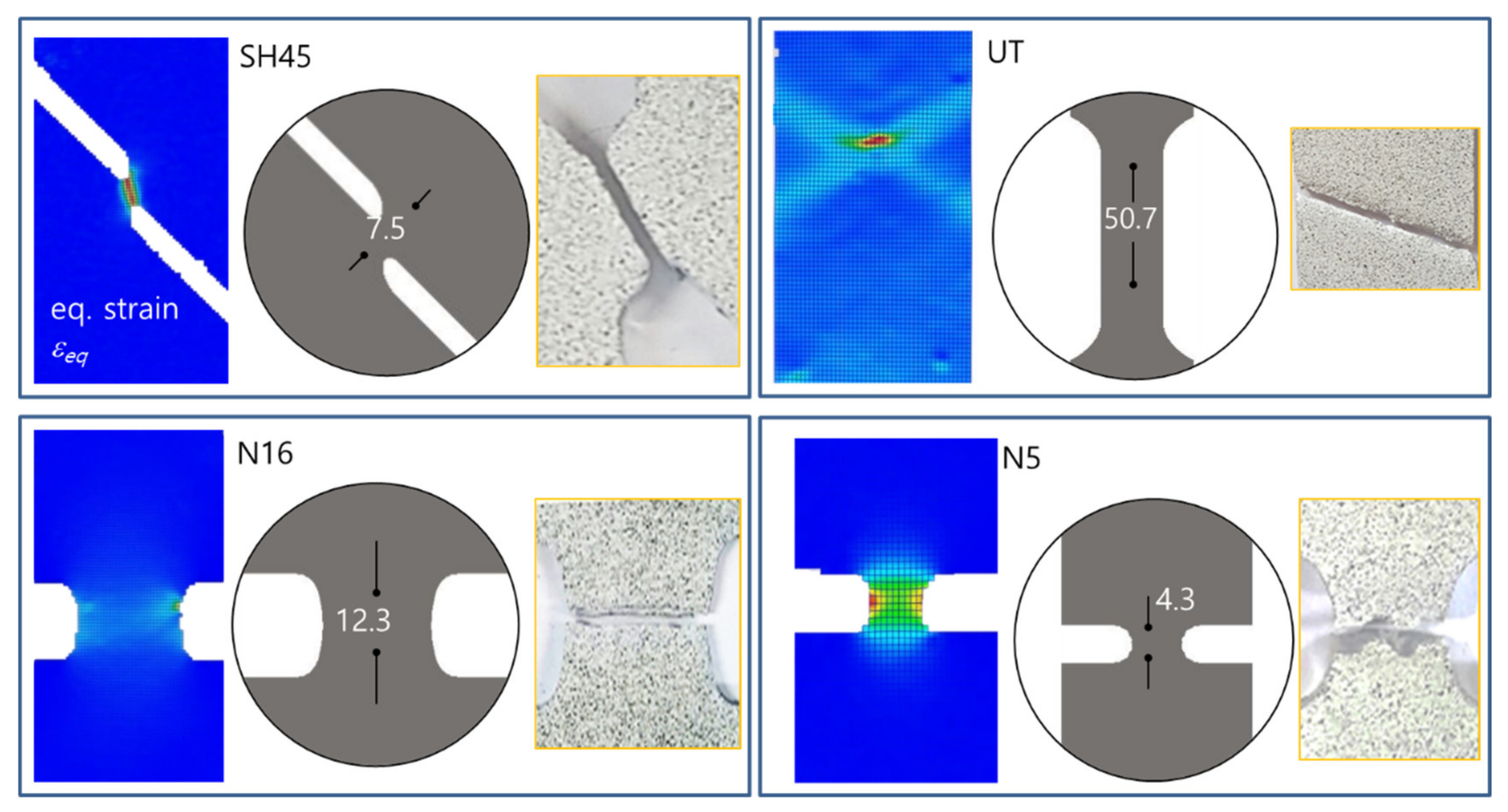
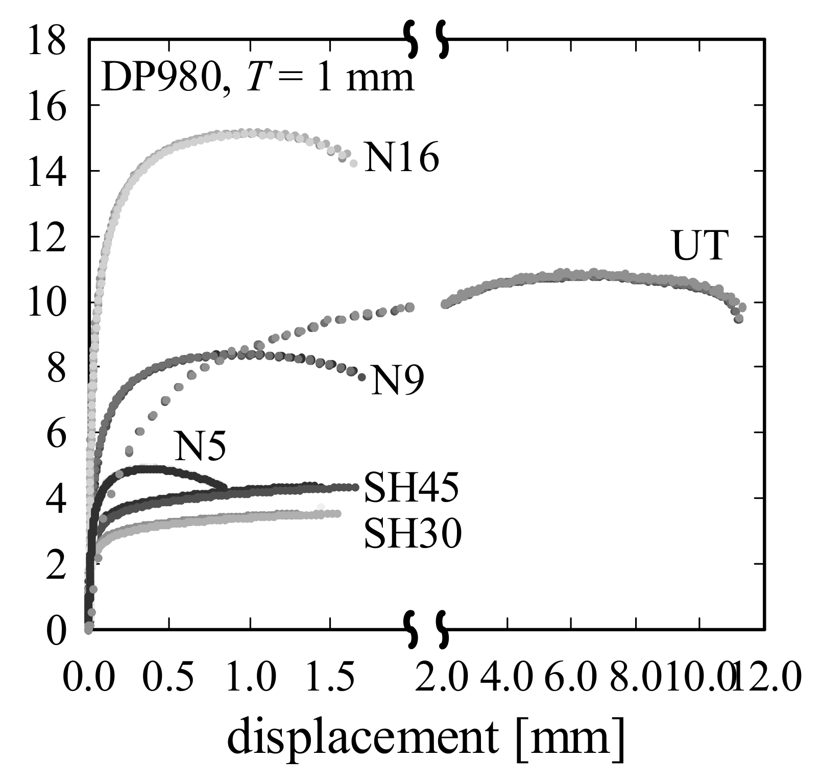
To impose the diverse loading modes necessary to establish the TFD in the region between pure shear and plane strain, the specimen geometries shown in Figure 3 were chosen; the failure regions of each specimen were subject to a constant η value, which will be determined in the next section. The specimens shown in 4 were mounted in a universal testing machine (UTM; Shimadzu AG-X, load capacity 50 kN) and loaded until failure, with a constant velocity of 5 mm/min (UT; uniaxial tension) and 3 mm/min (all of the others). The equivalent strain distribution in the specimen center and the fracture specimens are shown in Figure 4. The displacement data for the FD curves were obtained via DIC using virtual extensometers, and the gauge length for each specimen is the distance between the black points in Figure 4. Every test was performed three times so as to check repeatability. All of the experimental FD curves provided in Figure 5 show an excellent repeatability (as the curves for a certain specimen shape nearly coincide, the differences are difficult to discern).
3.2. Determination of Triaxiality η by DIC
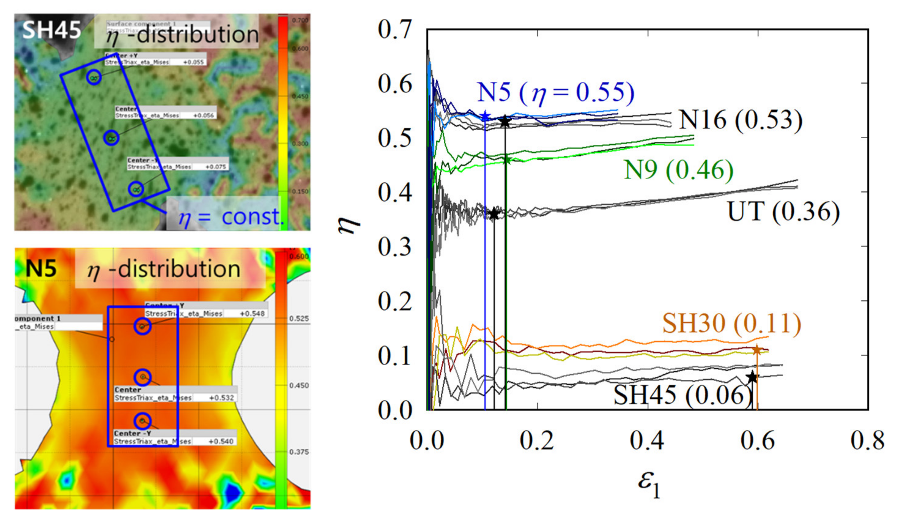
For establishing the TFD, we need to know the exact η-values for the single specimen shapes. To determine η, we extracted the principal strains at three locations on the specimen surface, as follows: one in the center, where the fracture occurs, and two approximately 1 mm off the center, as shown in Figure 6, for SH45 and N5. Based on the von Mises criterion, η was then calculated according to the following:
where σ1 is the maximum principal stress, and ε1 and ε2 are the in-plane maximum and minimum principal strains, respectively. The η-values are plotted over ε1 in the center in Figure 6. We observed that η is constant up to a maximum load, Fmax, and then starts increasing. However, as the increase is not pronounced, a representative η-value was determined by taking the average between ε1 = 0.04 and ε1 at Fmax. The problem of the η-increase was not considered here, but it is certainly something that needs more investigation, in particular, for materials more ductile than DP980. Using the average values, we found that η ranges between 0.06 and 0.55 (i.e., roughly between the pure shear and plane strain). Note that the actual η-values may differ from the theoretical ones (Figure 6), as anisotropy was disregarded here.
3.3. FE Modeling
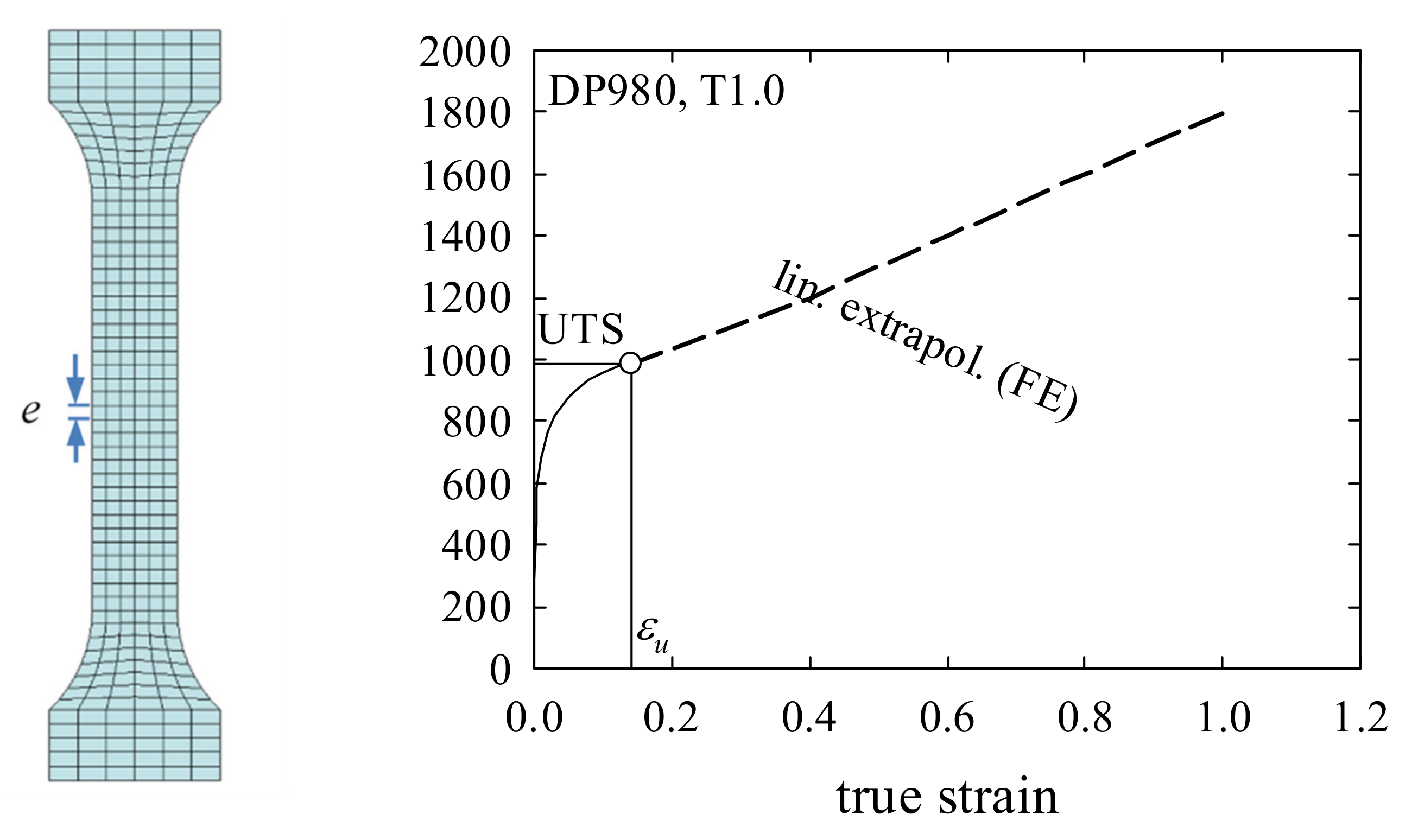
In addition, all of the tests were simulated in FE software LS-DYNA to determine the GISSMO parameters. The FE models were geometrically equal to the real specimens, with the exception that the clamped regions were not modeled. The bottom nodes were constrained in all directions, whereas the top nodes were only free to move in the loading direction. The meshes consisted of second order four-node shell elements with five through-thickness nodes, and the UT specimen FE model is shown in Figure 7. The reference edge length (e) was 2.0 mm, and for regularization, e varied between 0.8~4.0 mm.
The material was assumed to be isotropic (despite the sheet’s mild anisotropy) and obeyed Mises yielding and isotropic hardening (Young’s modulus of 210 GPa and Poisson’s ratio of 0.3). GISSMO was applied to model the damage. The average FD data obtained with the UT specimens (based on a gauge length of 50 mm) were converted to true stress–strain data, which served as an input to the finite element (FE) model (Figure 7). As the stress–strain data were only accurate up to stress at Fmax (denoted UTS = ultimate tensile strength), the data beyond the UTS were linearly extrapolated; the difference between the assumed and the real stress–strain curves was compensated for by applying GISSMO. A specimen was assumed to have failed once two elements lost their strength completely.
3.4. Determination of Damage Parameters through Optimization
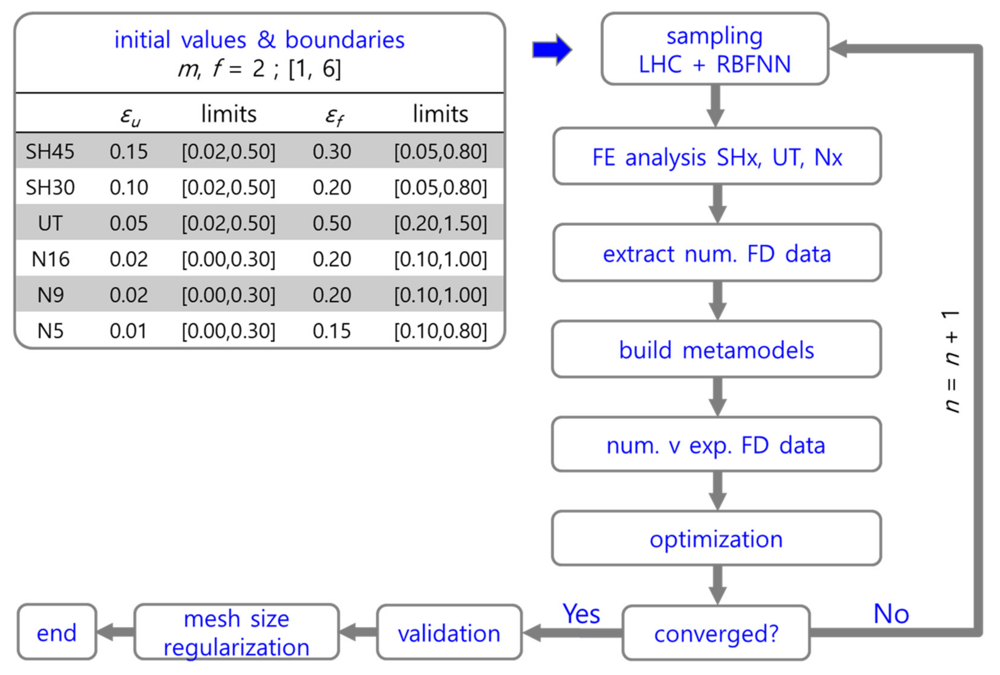
The damage parameters (εu, εf, m, and f) were determined by a metamodel-based optimization performed with LS-OPT. The initial values, together with the lower and upper boundaries for the damage parameters and the optimization flowchart, are given in Figure 8. The initial values for εu and εf were estimated from the experimental data (note that generally, the εf value for UT obtained through optimization differs from the one that would be achieved for the experimental data, because of different degrees of localness). The objective was to minimize, for all tensile tests (SHx, UT, and Nx), the total error between the numerical and experimental FD data, by applying the in-built curve matching algorithm. The numerical FD data were determined based on the same gauge length as that which was used in the tests (50 mm). First, a number of FE analyses were run, starting with the initial values and continuing with the sampled sets of damage parameters (LHC(Latin hypercube)and RBFNN(Radial Basis Function Neural Networks) sampling was used). The FD data were then extracted and compared with the experimental FD data, while a metamodel was being built. The total error (multi-objective) was computed, and the convergence (or not) was judged by comparing the error with the allowed error. If no convergence was reached, the next loop commenced by sampling and running further FE analyses. Once convergence was reached, further analyses were performed with mesh sizes of e = 0.8 and 4.0 mm, so as to mitigate mesh-dependence. The final damage parameters and the resulting TFD together with the regularization curve are shown Table 1 and Figure 9, respectively.
To validate the GISSMO parameters, all of the tests were performed with the final parameters. As Figure 10 reveals, the numerical FD curves were found to follow the experimental ones very closely. Only N16 showed some deviation from the experimental data.
4. Validation by Tearing of Adjusting Guide
For the validation of the material properties obtained in Section 3, a segment of an adjusting guide (thickness T = 1.0 mm) used in a vehicle was torn by a circular pin, sticking through the upper hole (Figure 11). The whole segment contained four holes, the centers of which were slightly off the vertical center line. The lower end was clamped, as depicted in Figure 11), where the lower two holes were hidden inside the lower clamp; during the test, the pin in the upper hole was displaced at a constant speed of 20 mm/min until failure. Again, DIC was employed to obtain the displacement and strain fields.
The numerical model consisted of 1400 second order shell elements, that is, the same type as that previously used in Section 3 (note that the damage parameters are only valid for this element type, and they cannot be used for others such as solid elements). The characteristic element length was e = 1.0 mm.
The validation of the material parameters was performed by comparing the (i) external force–displacement curves and (ii) the strain distributions at selected points obtained by experiment and FE analyses. An additional FE analysis was performed with the damage model deactivated to show the point where damage sets in. The externally applied force is plotted over the displacement (i.e., pin travel) in Figure 12. We can state that although the numerical analysis somewhat underestimated the maximum forces, the deviation was small (−5%), and the curves were of a similar shape. The first sharp decrease in load was due to the bulging of the hole rim, for which the pin was in contact with, in an out-of-plane direction, and was apparently not accompanied by damage. The subsequent “load arrest” between an approximately 8~10 mm displacement was very well reflected by the numerical analysis. The departure of the “no damage” curve from the “GISSMO” curve indicates the beginning of material weakening (i.e., D surpassed Dc). Furthermore, fracture occurred at approximately equal displacements (10.8 vs. 11.5 mm), although the exact failure displacement depends on numerous factors (for both experiment and FE analysis), and is therefore hard to predict.
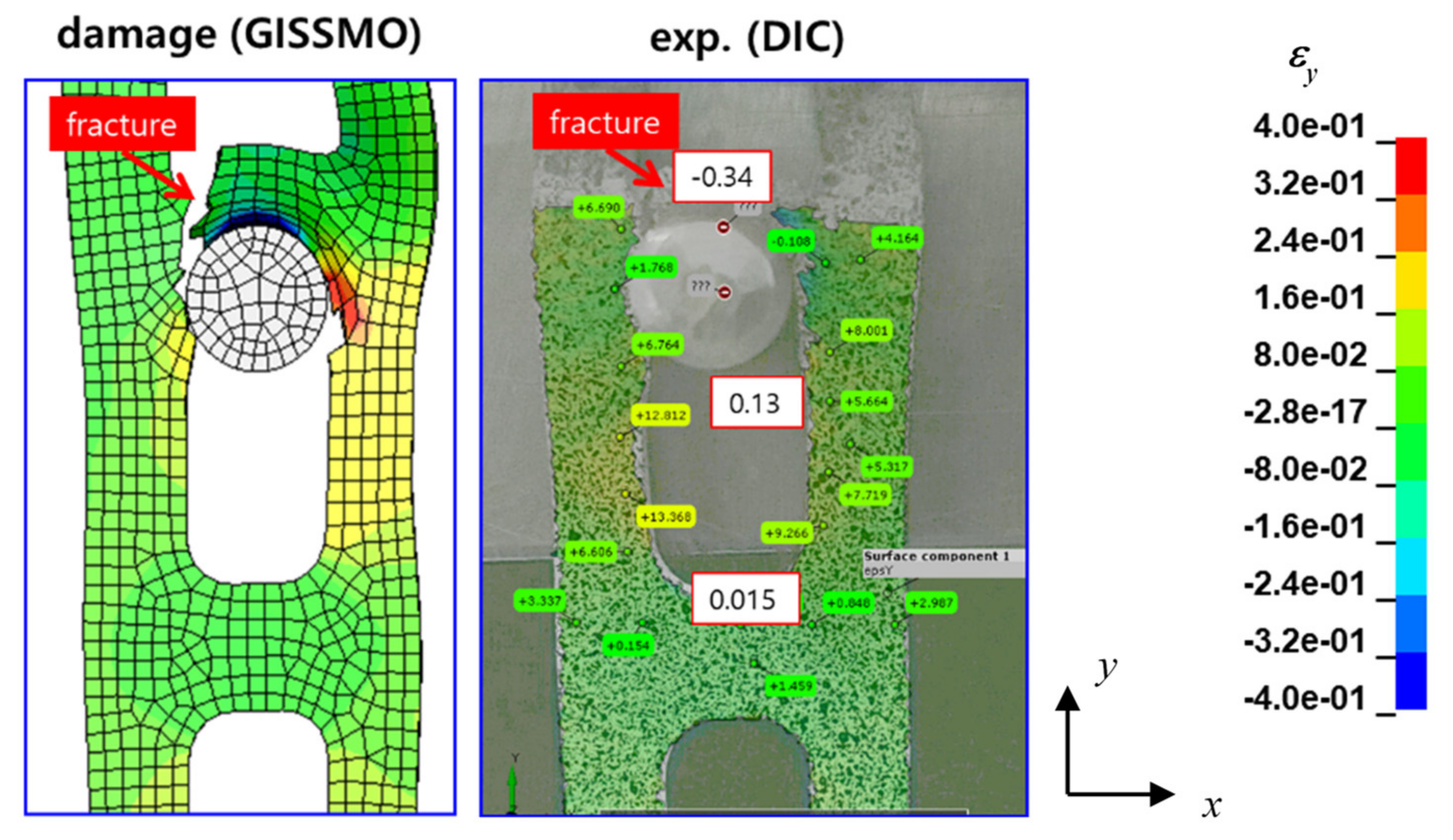
The equivalent strain distributions at fracture are shown in Figure 13. Crack formation was preceded by severe deformation. It was found that the maximum compressive strains in the y-direction (εy) in the part of the guide that was in contact with the pin were of a similar magnitude (−0.34 (test) vs. −0.38 (FE analysis)), and the values in the other regions were also in good agreement. Furthermore, for the experiment and simulation, the crack formed in the same region, namely on the left side of the ligament between two holes, which is subject to high strains, and grows in the y-direction.
The results show that the introduction of GISSMO facilitates quite a good reproduction of the experimental results. The presented FE model is proven to be applicable to complex cases, such as the one shown here. The discrepancies between the experiment and FE analysis may be explained by the neglect of the material anisotropy, which, despite the mild anisotropy of the sheets used here, may gain some significance under certain loading conditions. Furthermore, the rise of η with a plastic strain cannot be considered. However, the error in the externally applied maximum force is considered to be too small to justify an extensive investigation into the error’s possible origins, such as the compliance of a jig or frame, thickness variations in the strip, possible burrs around the holes, or friction.
5. Conclusions
In this paper, tensile tests with six specimen types were carried out. From the extracted FD data, fracture strains were obtained and the corresponding triaxialities were evaluated based on the local strain data so as to eventually establish the TFD for DP980 (necking and fracture) for the range of η = 0~0.55. Details on how the damage model parameters could be derived efficiently by reverse engineering-based optimization were given. The material properties were finally validated by tearing an adjusting guide using a pin until failure.
It was found that DIC is an excellent tool for determining a representative η for a given specimen shape, and that by applying GISSMO, the experimental results could be reproduced with a high accuracy. Experiment and FE analysis gave similar external load–displacement curves. The fracture displacement and locus were predicted accurately, and the local strain distributions were also in good agreement. This shows that the material model and the model parameters obtained here can be applied to complex deformation processes. Nonetheless, more validation studies are needed in order to further substantiate this claim, and to tackle the problem of the η-increase with strain.
Author Contributions
Data curation, S.H.; investigation, S.H. and J.K.; resources, T.J.; writing (original draft), S.H.
Funding
This research received no external funding.
Conflicts of Interest
The authors declare no conflict of interest. The funders had no role in the design of the study; in the collection, analyses, or interpretation of data; in the writing of the manuscript; or in the decision to publish the results.
References
- Cockcroft, M.G.; Latham, D.J. Ductility and the workability of metals. J. Inst. Met. 1968, 96, 33–39. [Google Scholar]
- Oh, S.I.; Chen, C.C.; Kobayashi, S. Ductile fracture in axisymmetric extrusion and drawing: Part 2 workability in extrusion and drawing. J. Manuf. Sci. Eng. Trans. ASME 1979, 101, 36–44. [Google Scholar] [CrossRef]
- Oyane, M.; Sato, T.; Okimoto, K.; Shima, S. Criteria for ductile fracture and their applications. J. Mech. Work. Technol. 1980, 4, 65–81. [Google Scholar] [CrossRef]
- Gurson, A.L. Continuum theory of ductile rupture by void nucleation and growth. J. Eng. Mater. Technol. 1977, 99, 2–15. [Google Scholar] [CrossRef]
- Johnson, G.R.; Cook, W.H. Fracture characteristics of three metals subjected to various strains, strain rates, temperatures and pressures. Eng. Fract. Mech. 1985, 21, 31–48. [Google Scholar] [CrossRef]
- McClintock, F.A. A Criterion for Ductile Fracture by the Growth of Holes. J. Appl. Mech. 1968, 35, 363–371. [Google Scholar] [CrossRef]
- Rice, J.R.; Tracey, D.M. On the ductile enlargement of voids in triaxial stress fields. J. Mech. Phys. Solids 1969, 17, 201–217. [Google Scholar] [CrossRef] [Green Version]
- Bai, Y.; Wierzbicki, T. Application of extended Mohr–Coulomb criterion to ductile fracture. Int. J. Fract. 2010, 161, 1–20. [Google Scholar] [CrossRef]
- Neukamm, F.; Feucht, M.; Haufe, A. Consistent damage modelling in the process chain of forming to crashworthiness simulations. LS DYNA Anwend. 2008, 30, 11–20. [Google Scholar]
- Neukamm, F.; Feucht, M.; Haufe, A.; Ag, D. Considering damage history in crashworthiness simulations. In Proceedings of the 7th European LS-DYNA Conference, Salzburg, Austria, 14–15 May 2009. [Google Scholar]
- Livermore Software Technology Corporation. LS-DYNA Keyword User’s Manual, R9.0; Livermore Software Technology Corporation: Livermore, CA, USA, 2016; ISBN 9254492507. [Google Scholar]
- Schauwecker, F.; Moncayo, D.; Andrade, F.; Feucht, M. Modeling of Bolts using the GISSMO Model for Crash Analysis. In Proceedings of the 12th European LS-DYNA Conference, Koblenz, Germany, 14–16 May 2019. [Google Scholar]
- ARAMIS. Manual Aramis Professional 2018; GOM-Gesellschaft für Optische Messtechnik mbH: Braunschweig, Germany, 2018. [Google Scholar]
- Effelsberg, J.; Haufe, A.; Feucht, M.; Neukamm, F.; Bois, P. Du On parameter identification for the GISSMO damage model. In Proceedings of the 12th International LS-DYNA Users Conference, Detroit, MI, USA, 3–5 June 2012; pp. 1–12. [Google Scholar]
Figure 1.
Acquisition of load and local deformations by universal testing machine (UTM) and GOM Aramis.
Figure 1.
Acquisition of load and local deformations by universal testing machine (UTM) and GOM Aramis.

Figure 2.
Possible η-dependences of εu and εf under plane stress conditions (triaxiality failure diagram (TFD)); the runs are examples and may differ from one material to the next.
Figure 2.
Possible η-dependences of εu and εf under plane stress conditions (triaxiality failure diagram (TFD)); the runs are examples and may differ from one material to the next.

Figure 3.
Specimen shapes; all dimensions in mm.

Figure 4.
Equivalent strain distributions as in GOM Aramis; surface points on which FD data are derived (for SH30 and N9, see SH45 and N16, respectively); fractured specimens.
Figure 4.
Equivalent strain distributions as in GOM Aramis; surface points on which FD data are derived (for SH30 and N9, see SH45 and N16, respectively); fractured specimens.

Figure 5.
Force–displacement (FD) data from all of the tests, with three tests per specimen type.

Figure 6.
η-distribution prior to fracture in SH45 and N5, and η-history in the diverse specimens; star symbols denote Fmax.
Figure 6.
η-distribution prior to fracture in SH45 and N5, and η-history in the diverse specimens; star symbols denote Fmax.

Figure 7.
UT specimen (e = 2.0 mm; left); true stress–strain data converted from UT FD data to Fmax and then linearly extrapolated, serves as the finite element (FE) input (right).
Figure 7.
UT specimen (e = 2.0 mm; left); true stress–strain data converted from UT FD data to Fmax and then linearly extrapolated, serves as the finite element (FE) input (right).

Figure 8.
Optimization procedure, including regularization.

Figure 9.
TFD (left) and mesh dependence (right).

Figure 10.
Experimental average FD curves and numerical FD curves obtained with the final damage parameters.
Figure 10.
Experimental average FD curves and numerical FD curves obtained with the final damage parameters.

Figure 11.
Test setup for adjusting the guide tearing: as in GOM Aramis (left) and the model (right).
Figure 11.
Test setup for adjusting the guide tearing: as in GOM Aramis (left) and the model (right).

Figure 12.
External FD curves from experiment and numerical analysis with and without consideration of damage.
Figure 12.
External FD curves from experiment and numerical analysis with and without consideration of damage.

Figure 13.
Comparison of εy distributions obtained by experiment and FE analysis.


Table 1.
Final damage parameters from optimization.
| DP980 | η | εu | εf | m | f |
|---|---|---|---|---|---|
| SH45 | 0.06 | 0.219 | 0.257 | 1.206 | 5.249 |
| SH30 | 0.11 | 0.040 | 0.156 | ||
| UT | 0.36 | 0.022 | 0.590 | ||
| N9 | 0.48 | 0.010 | 0.341 | ||
| N16 | 0.53 | 0.010 | 0.316 | ||
| N5 | 0.55 | 0.010 | 0.272 |
© 2019 by the authors. Licensee MDPI, Basel, Switzerland. This article is an open access article distributed under the terms and conditions of the Creative Commons Attribution (CC BY) license (http://creativecommons.org/licenses/by/4.0/).
Share and Cite
MDPI and ACS Style
Hong, S.; Kim, J.; Jun, T. Failure Prediction for the Tearing of a Pin-Loaded Dual Phase Steel (DP980) Adjusting Guide. Appl. Sci. 2019, 9, 5460. https://doi.org/10.3390/app9245460
AMA Style
Hong S, Kim J, Jun T. Failure Prediction for the Tearing of a Pin-Loaded Dual Phase Steel (DP980) Adjusting Guide. Applied Sciences. 2019; 9(24):5460. https://doi.org/10.3390/app9245460
Chicago/Turabian StyleHong, Seokmoo, Jinkyoo Kim, and Taehwan Jun. 2019. "Failure Prediction for the Tearing of a Pin-Loaded Dual Phase Steel (DP980) Adjusting Guide" Applied Sciences 9, no. 24: 5460. https://doi.org/10.3390/app9245460
Note that from the first issue of 2016, this journal uses article numbers instead of page numbers. See further details here.